Electric structure of shallow D-wave states in Halo EFT

Abstract

We compute the electric form factors of one-neutron halo nuclei with shallow $D$-wave states up to next-to-leading order and the E2 transition from the $S$-wave to the $D$-wave state up to leading order in Halo Effective Field Theory (Halo EFT). The relevant degrees of freedom are the core and the halo neutron. The EFT expansion is carried out in powers of $R_{core}/R_{halo}$, where $R_{core}$ and $R_{halo}$ denote the length scales of the core and the halo, respectively. We propose a power counting scenario for weakly-bound states in one-neutron Halo EFT and discuss its implications for higher partial waves in terms of universality. The scenario is applied to the $\frac{5}{2}^{+}$ first excited state and the $\frac{1}{2}^{+}$ ground state of ¹⁵C. We obtain several universal correlations between electric observables and use data for the E2 transition $\frac{5}{2}^{+}\to\frac{1}{2}^{+}$ together with ab initio results from the No-Core Shell Model to predict the quadrupole moment.

I Introduction

The quantitative description of halo nuclei in Halo Effective Field Theory (Halo EFT) provides insights into their universal properties. Halo nuclei consist of a tightly bound core nucleus surrounded by one or more weakly bound nucleons Jensen et al. (2004); Riisager (2013). This separation of scales can be captured in terms of the core length scale, $R_{core}$, and the halo scale, $R_{halo}$, with $R_{halo}\gg R_{core}$. Halo EFT exploits this separation of scales to describe halo nuclei Bertulani et al. (2002); Bedaque et al. (2003). In this approach, the relevant degrees of freedom are the core and the halo nucleons. Halo EFT is complementary to ab initio methods that have difficulties describing weakly-bound states and provides a useful tool to identify universal correlations between observables. For recent reviews of Halo EFT see Refs. Ando (2016); Rupak (2016); Hammer et al. (2017).

The Halo EFT formalism has been successfully used to study various reactions and properties of halo-like systems. Some early examples in the strong sector include the $n\alpha$ resonance in ⁵He Bertulani et al. (2002); Bedaque et al. (2003) the $\alpha\alpha$ resonance in ⁸Be Higa et al. (2008) and universal properties, matter form factors and radii of two-neutron halo nuclei with predominantly $S$-wave Canham and Hammer (2008, 2010) and $P$-wave interactions Rotureau and van Kolck (2013); Ji et al. (2014). Due to the importance of higher partial waves in halo nuclei, different power counting schemes are conceivable that have a varying number of fine tuned parameters Bertulani et al. (2002); Bedaque et al. (2003). From naturalness assumptions, one expects a lower number of fine tunings to be more likely to occur in nature. However, the level of fine tuning depends strongly on the details of the considered system and has to be verified and adjusted to data.

In Halo EFT, electromagnetic interactions can be straightforwardly included via minimal substitution in the Lagrangian, and relevant electromagnetic currents can be added. Some applications to one-neutron halos, which we consider here, are the calculation of electric properties of ¹¹Be Hammer and Phillips (2011), ¹⁵C Fernando et al. (2015), radiative neutron capture on ⁷Li Rupak and Higa (2011); Zhang et al. (2014a) and ¹⁴C Rupak et al. (2012), the ground state structure of ¹⁹C Acharya and Phillips (2013), and the electromagnetic properties of ¹⁷C Braun et al. (2018). The parameters needed as input in Halo EFT can be either taken from experiment or from ab initio calculations Hagen et al. (2013); Zhang et al. (2014b, a), which shows the versatility and complementary character of Halo EFT.

Electric properties provide a unique window on the structure and dynamics of one-neutron halo nuclei. In this work, we consider ¹⁵C as an example and follow the approach presented in Ref. Hammer and Phillips (2011), where electric properties of ¹¹Be are calculated using Halo EFT. ¹⁵C also has two bound states. The $\frac{1}{2}^{+}$ ground state of ¹⁵C is predominantly an $S$-wave bound state, and the $\frac{5}{2}^{+}$ first excited state predominantly a $D$-wave bound state. Therefore, we focus on the extension to partial waves beyond the $P$-wave, in general, and especially on the extension to $D$-wave states. We include the strong $D$-wave interaction by introducing a new dimer field and compute the E2 transition strength and electric form factors. In the context of the strong $d+t\leftrightarrow n+\alpha$ reaction, $D$-wave states were also investigated in Ref. Brown and Hale (2014). We use a similar approach for dressing the $D$-wave propagator, but a different regularization scheme. This entails a different power counting scheme as will be discussed in more detail in the next section.

The paper is organized as follows: After writing down the non-relativistic Lagrangian for the $S$- and $D$-wave case in Section II, we dress the $S$- and $D$-wave propagators. As regularization scheme, a momentum cutoff is employed to identify all divergences. For practical calculations, the power divergence subtraction scheme Kaplan et al. (1998a, b) is applied for convenience. Based on our analysis of the divergence structure, we propose a power counting scenario and discuss its implications for higher partial wave bound states in terms of universality. In Ref. Braun et al. (2018), the same power counting as in this paper is applied in order to describe shallow $D$-wave bound states in ¹⁷C. After the inclusion of electric interactions in our theory, the B(E2) transition strength between the $S$- and $D$-wave state as well as electric form factors of the $D$-wave state are calculated in Section III. First, we present general results and correlations for such weakly-bound systems and then apply them to the case of ¹⁵C. Eventually, our Halo EFT results for ¹⁵C are combined with data for the B(E2) transition strength Ajzenberg-Selove (1986) and ab initio results from the Importance-Truncated No-Core Shell Model (IT-NCSM) Roth (2009). In this way, we are able to predict the quadrupole and hexadecapole moments and radii. Our findings are then compared to correlations Calci and Roth (2016a) which are motivated by the rotational model of Bohr and Mottelson Bohr and Mottelson (1975). In Section IV, we present our conclusions.

II Halo EFT formalism

We apply the Halo EFT formalism for the electric properties of $P$-wave systems developed in Ref. Hammer and Phillips (2011) to shallow $D$-wave systems. Since we use our theory to describe ¹⁵C which has a shallow $S$-wave state ($J^{P}=\frac{1}{2}^{+}$) and a shallow $D$-wave state ($J^{P}=\frac{5}{2}^{+}$), we also include an $S$-wave state in our theory.

II.1 Lagrangian

The relevant degrees of freedom are the core, a bosonic field $c$, and the halo neutron, a spinor field $n$. The strong $S$- and $D$-wave interactions are included through auxiliary spinor fields $\sigma$ for the $S$-wave state and $d$ for the $D$-wave states, respectively. Note, that we include only one $d$ field in the Lagrangian below. In principle, there are two $d$ fields for the $\frac{5}{2}^{+}$ and $\frac{3}{2}^{+}$ states, respectively. Summing over repeated spin indices, the effective Lagrangian can be written as

$$\mathcal{L}=\ c^{\dagger}\left(i\partial_{t}+\frac{\nabla^{2}}{2M}\right)c+n^{\dagger}\left(i\partial_{t}+\frac{\nabla^{2}}{2m_{n}}\right)n+\sigma_{s}^{\dagger}\left[\eta_{0}\left(i\partial_{t}+\frac{\nabla^{2}}{2M_{nc}}\right)+\Delta_{0}\right]\sigma_{s}$$

$$+d_{m}^{\dagger}\left[c_{2}\left(i\partial_{t}+\frac{\nabla^{2}}{2M_{nc}}\right)^{2}+\eta_{2}\left(i\partial_{t}+\frac{\nabla^{2}}{2M_{nc}}\right)+\Delta_{2}\right]d_{m}$$

$$-g_{0}\left[c^{\dagger}n_{s}^{\dagger}\sigma_{s}+\sigma_{s}^{\dagger}n_{s}c\right]-g_{2}^{J}\left[d^{\dagger}_{m}\left[n\overset{\leftrightarrow}{\nabla}^{2}c\right]_{J,m}+\left[c^{\dagger}\overset{\leftrightarrow}{\nabla}^{2}n^{\dagger}\right]_{J,m}d_{m}\right]+\ldots\ ,$$ (1)

where $3/2\leq J\leq 5/2$ denotes the total spin of the $D$-wave state, $m_{n}$ is the neutron mass, $M$ the core mass and $M_{nc}=m_{n}+M$ is the total mass of the $nc$ system. The repeated spin indices $s$ and $m$ are summed over according to the Einstein convention. The power counting for this Lagrangian depends on the underlying scales and will be discussed below. The $S$-wave part of Eq. (1) contains three coupling constants $g_{0}$, $\Delta_{0}$ and $\eta_{0}$, while only two of them are linearly independent. In principle, we are free to choose which constant is set to a fixed value. Here, we choose $\eta_{0}=\pm 1$ to be a sign which will be fixed by the effective range. (For an alternative choice, see Ref. Griesshammer (2004).) This part is well known and has been discussed extensively in the literature on Halo EFT Hammer et al. (2017); Hammer and Phillips (2011); Fernando et al. (2015). To make the paper self-contained, the key equations for the interacting propagator of the $S$-wave state are collected in Appendix A. In the following, we focus on the properties of the $D$-wave state. For the $D$-wave, we include four constants in our Lagrangian, namely $c_{2}$, $\eta_{2}$, $\Delta_{2}$ and $g_{2}$. However, in this case only three of them are linearly independent. Again, we are free to choose which constant is set to a fixed value. Here, we choose $\eta_{2}=\pm 1$ to be a sign, but other choices are possible. The additional 2nd-order kinetic term with constant $c_{2}$ is needed to renormalize the interacting $D$-wave propagator which contains up to quintic divergences. Since the core and neutron have different masses, it is convenient to define the interaction terms with Galilei invariant derivatives

$$n\overset{\leftrightarrow}{\nabla}c=n\ \frac{\left(M\overset{\leftarrow}{\nabla}-m_{n}\overset{\rightarrow}{\nabla}\right)}{M_{nc}}\ c\ ,$$ (2)

where the arrows indicate the direction of their action. We project on the $J=5/2$ or $3/2$ component of the interaction by defining

$$\left[n\overset{\leftrightarrow}{\nabla}^{2}c\right]_{J,m}=\sum_{m_{s}m_{l}}\left(\left.\frac{1}{2}m_{s}\ 2m_{l}\right|Jm\right)\ n_{m_{s}}\sum_{\alpha\beta}\left(\left.1\alpha\ 1\beta\right|2m_{l}\right)\frac{1}{2}\left(\overset{\leftrightarrow}{\nabla}_{\alpha}\overset{\leftrightarrow}{\nabla}_{\beta}+\overset{\leftrightarrow}{\nabla}_{\beta}\overset{\leftrightarrow}{\nabla}_{\alpha}\right)\ c\ ,$$ (3)

where $\alpha$ and $\beta$ are spherical indices and $\left(\left.j_{1}m_{1}\ j_{2}m_{2}\right|Jm\right)$ are Clebsch-Gordan coefficients Tanabashi et al. (2018) coupling $j_{1}$ and $j_{2}$ with projections $m_{1}$ and $m_{2}$, respectively, to $J$ with projection $m$.

In practice, we calculate $D$-wave observables in Cartesian coordinates and then couple the spin and relative momentum in the appropriate way. For better distinction, we use Greek indices for the spherical representation and Latin indices for the Cartesian representation throughout this paper. The Cartesian form of the strong $D$-wave interaction is taken from Refs. Bedaque et al. (2003); Brown and Hale (2014)

$$\frac{1}{2}\left(\overset{\leftrightarrow}{\nabla}_{i}\overset{\leftrightarrow}{\nabla}_{j}+\overset{\leftrightarrow}{\nabla}_{j}\overset{\leftrightarrow}{\nabla}_{i}\right)-\frac{1}{\mathrm{d}-1}\overset{\leftrightarrow}{\nabla}^{2}\delta_{ij}\ ,$$ (4)

where $\mathrm{d}$ denotes the space-time dimension. This interaction yields 9 components, but a straightforward check shows that only 5 of them are linearly independent. Thus, the $D$-wave part of the Lagrangian (4) is Galilei invariant and contains the correct number of degrees of freedom.

The relation between spherical and cartesian coordinates is given by

$$r_{\pm 1}=\mp(x_{1}\pm ix_{2})/\sqrt{2}\,,\quad r_{0}=x_{3}\,,$$ (5)

and similar relations apply to other quantities. For convenience, we will always use the Cartesian representation, but we will switch to a spherical basis if a coupling to definite angular momentum is required.

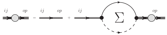
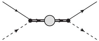
Figure 1: The dashed line denotes the core field $c$ and the thin solid line the neutron. The thin double line represents the bare dimer propagator and the thick double line with the gray circle is the dressed dimer propagator. The top panel shows the diagrammatic representation of the Dyson equation for the dressed dimer propagator and the bottom panel the neutron-core scattering amplitude with the dressed dimer propagator.

II.2 D-wave propagator

The dressed $d$ propagator and the $D$-wave scattering amplitude are computed from summing the bubble diagrams in Fig. 1. This corresponds to the exact solution of the field theory defined by the terms explicitly shown in Eq. (1) for the $D$-wave state. In the next subsection, we will develop a power counting scheme that classifies the different contributions to the propagator according to their importance at low energies. After this scheme has been established, only the terms contributing to the considered order will be included. To make the divergence structure transparent, we will use a simple momentum cutoff to regularize the loop integrals. As before, we calculate the dressed $D$-wave propagator in the Cartesian representation and couple the neutron spin and the relative momentum to project out the appropriate angular momentum $J$ in the end. The Dyson equation for the $D$-wave is illustrated in the top panel of Fig. 1 and yields

$$D_{d}(p)_{ijop} =D_{d}(p)\ \frac{\left(\delta_{io}\delta_{jp}+\delta_{ip}\delta_{jo}-\frac{2}{3}\delta_{ij}\delta_{op}\right)}{2}\ ,$$ (6)

$$D_{d}(p) =\frac{1}{\Delta_{2}+\eta_{2}\left[p_{0}-\mathbf{p}^{2}/(2M_{nc})\right]+c_{2}\left[p_{0}-\mathbf{p}^{2}/(2M_{nc})\right]^{2}-\Sigma_{d}(p)}\ ,$$ (7)

with the one-loop self-energy

$$\Sigma_{d}(p)_{ijop}= \Sigma_{d}(p)\ \frac{\left(\delta_{io}\delta_{jp}+\delta_{ip}\delta_{jo}-\frac{2}{3}\delta_{ij}\delta_{op}\right)}{2}\ ,$$ (8)

$$\Sigma_{d}(p)= -\frac{m_{R}g_{2}^{2}}{15\pi}\left[\frac{2}{5\pi}\Lambda^{5}+\frac{2}{3\pi}(2m_{R})\left(p_{0}-\frac{p^{2}}{2M_{nc}}\right)\Lambda^{3}+\frac{2}{\pi}(2m_{R})^{2}\left(p_{0}-\frac{p^{2}}{2M_{nc}}\right)^{2}\Lambda\right.$$

$$\left.+i(2m_{R})^{5/2}\left(p_{0}-\frac{p^{2}}{2M_{nc}}\right)^{5/2}\right]\ ,$$ (9)

where $m_{R}=(m_{n}M)/(m_{n}+M)$ denotes the reduced mass of the neutron-core system and $\Lambda$ is a momentum cutoff. In spherical coordinates the Cartesian tensor Brown and Hale (2014)

$$\frac{\left(\delta_{io}\delta_{jp}+\delta_{ip}\delta_{jo}-\frac{2}{3}\delta_{ij}\delta_{op}\right)}{2}\leavevmode\nobreak\ ,$$ (10)

transforms to

$$\sum_{\alpha\beta\gamma\delta}\left(\left.1\alpha\ 1\beta\right|2m_{l}\right)\left(\left.1\gamma\ 1\delta\right|2m_{l}^{\prime}\right)\frac{\left(\delta_{\alpha\gamma}\delta_{\beta\delta}+\delta_{\alpha\delta}\delta_{\beta\gamma}+\delta_{\alpha-\beta}(-1)^{\beta}\delta_{\gamma-\delta}(-1)^{\delta}\right)}{2}\ =\delta_{m_{l},m_{l}^{\prime}}\ ,$$ (11)

and eventually, the full angular momentum coupling (3) applied in the incoming and outgoing channel yields

$$\Sigma_{d}(p)_{mm^{\prime}} =\sum_{m_{s}m_{l}m_{s}^{\prime}m_{l}^{\prime}}\left(\left.\frac{1}{2}m_{s}\ 2m_{l}\right|Jm\right)\left(\left.\frac{1}{2}m_{s}^{\prime}\ 2m_{l}^{\prime}\right|Jm^{\prime}\right)\delta_{m_{l}m_{l}^{\prime}}\delta_{m_{s}m_{s}^{\prime}}\Sigma_{d}(p)=\delta_{mm^{\prime}}\Sigma_{d}(p)\ ,$$ (12)

where $m_{s}$ $(m_{s}^{\prime})$ and $m_{l}$ $(m_{l}^{\prime})$ are the spin projections of the created (annihilated) neutron and the projections of the $D$-wave interaction at both vertices of the bubble diagram in Fig. 1, respectively. Moreover, $J$ denotes the total spin with its incoming and outgoing projections $m$ and $m^{\prime}$, respectively. The $D$-wave scattering amplitude in the two-body center-of-mass frame with $E=k^{2}/(2m_{R})$ and $k=|\mathbf{p}^{\prime}|=|\mathbf{p}|$ for on-shell scattering

$$t_{2}(\mathbf{p}^{\prime},\mathbf{p};E)=g_{2}^{2}\left[\left(\mathbf{p}\cdot\mathbf{p}^{\prime}\right)^{2}-\frac{1}{3}\mathbf{p}^{2}\mathbf{p}^{\prime 2}\right]D_{d}(E,\mathbf{0})\ ,$$ (13)

is matched to the effective range expansion

$$t_{2}(\mathbf{p}^{\prime},\mathbf{p};E)=\frac{15\pi}{m_{R}}\frac{\left(\mathbf{p}\cdot\mathbf{p}^{\prime}\right)^{2}-\frac{1}{3}\mathbf{p}^{2}\mathbf{p}^{\prime 2}}{1/a_{2}-\frac{1}{2}r_{2}k^{2}+\frac{1}{4}\mathcal{P}_{2}k^{4}+ik^{5}}\ ,$$ (14)

and we find the matching relations

$$\frac{1}{a_{2}}=\frac{15\pi}{m_{R}g_{2}^{2}}\Delta_{2}+\frac{2}{5\pi}\Lambda^{5}\ ,\quad r_{2}=-\frac{15\pi}{m_{R}^{2}g_{2}^{2}}\eta_{2}-\frac{2}{3\pi}\Lambda^{3}\ ,\quad\mathcal{P}_{2}=\frac{15\pi}{m_{R}^{3}g_{2}^{2}}c_{2}+\frac{2}{\pi}\Lambda\ ,$$ (15)

which determine the running of the coupling constants $g_{2}$, $\Delta_{2}$, and $c_{2}$ with the cutoff $\Lambda$. Since we get $\Lambda$ dependencies with powers of $5$, $3$, and $1$, the effective range parameters $a_{2}$, $r_{2}$, and $\mathcal{P}_{2}$ are required for renormalization at LO. This pattern motivates our power counting scheme discussed below. In particular, we include the 2nd-order kinetic term proportional to $c_{2}$ (cf. Ref Beane and Savage (2001)) in (1) in order to absorb the quintic divergence. If the values for these ERE parameters are known, they can be used to fix the EFT couplings $\Delta_{2}$, $c_{2}$ and $g_{2}$ in our theory. In the vicinity of the bound state pole, the dressed $d$ propagator can be written as

$$D_{d}(p) =Z_{d}\ \frac{1}{p_{0}-\frac{\mathbf{p}^{2}}{2M_{nc}}+B_{2}}+R_{d}(p)\ ,$$

$$Z_{d} =-\frac{15\pi}{m_{R}^{2}g^{2}_{2}}\ \frac{1}{r_{2}+\mathcal{P}_{2}\gamma_{2}^{2}-5\gamma_{2}^{3}}\ ,$$ (16)

where $Z_{d}$ denotes the wave-function renormalization, $B_{2}=\gamma_{2}^{2}/(2m_{R})$ denotes the binding energy with the binding momentum $\gamma_{2}\sim 1/R_{halo}$, and $R_{d}(p)$ is the remainder which is regular at the pole. The pole condition gives the relation between the effective range parameters $a_{2}$, $r_{2}$, $\mathcal{P}_{2}$ and the binding momentum $\gamma_{2}$

$$\frac{1}{a_{2}}+\frac{1}{2}r_{2}\gamma_{2}^{2}+\frac{1}{4}\mathcal{P}_{2}\gamma_{2}^{4}=0\ .$$ (17)

II.3 Power counting

For the shallow $S$-wave state, we adopt the standard power counting from pionless EFT van Kolck (1997, 1999); Kaplan et al. (1998a, b). This implies the scaling $1/\gamma_{0}\sim a_{0}\sim R_{halo}$ and $r_{0}\sim R_{core}$, where $\gamma_{0}=(1-\sqrt{1-2r_{0}/a_{0}})/r_{0}$ is the bound/virtual state pole position, $a_{0}$ the scattering length, and $r_{0}$ the effective range. As a result, $r_{0}$ contributes at next-to-leading order (NLO) in the expansion in $R_{core}/R_{halo}$.

Because more effective range parameters are involved, the power counting for shallow states in higher partial waves is not unique and different scenarios are conceivable Bertulani et al. (2002); Bedaque et al. (2003). We apply the constraint that our scheme should exhibit the minimal number of fine tunings in the coupling constants required to absorb all power law divergences. This is motivated by the expectation that every additional fine tuning makes a scenario less likely to be found in nature, as discussed by Bedaque et al. in Ref. Bedaque et al. (2003). They explicitly consider $P$-waves where both $a_{1}$ and $r_{1}$ enter at leading order (LO) and assume the scaling relations $a_{1}\sim R_{halo}^{2}R_{core}$ and $r_{1}\sim 1/R_{core}$, while higher effective range parameters scale with the appropriate power of $R_{core}$. This scenario requires only one fine-tuned combination of coupling constants in contrast to the alternative scenario proposed in Ref. Bertulani et al. (2002) which requires two. In this work, we follow the general arguments of Ref. Bedaque et al. (2003) and apply them to the $D$-wave case.

To renormalize all divergences in the $D_{d}(p)$ propagator, Eq. (6), the effective range parameters $a_{2}$, $r_{2}$, and $\mathcal{P}_{2}$ are all required. In the minimal scenario thus two out of three combinations of coupling constants need to be fine-tuned, i.e. $a_{2}\sim R_{halo}^{4}\ R_{core}$ and $r_{2}\sim 1/(R_{halo}^{2}\ R_{core})$, while $\mathcal{P}_{2}\sim 1/R_{core}$. With this scaling, all three terms contribute at the same order for typical momenta $k\sim 1/R_{halo}$. Higher effective range parameters scale with $R_{core}$ only and thus are suppressed by powers of $R_{core}/R_{halo}$.

This means that the dominant contribution to the $D$-wave bound state, after resumming all bubble diagrams and appropriate renormalization, comes from the bare propagator. In particular, the general structure of the propagator near the bound state pole at $E=-B_{d}$,

$$D_{d}(E)=\frac{Z_{d}}{E+B_{d}}\quad+\quad\mbox{regular terms in $E$}\,,$$ (18)

with $Z_{d}$ the wave function renormalization constant, is fully reproduced by the bare $D$-wave propagator. Furthermore, all imaginary parts, if present, appear in the regular part of the amplitude. With our assumptions about the scaling of $a_{2}$, $r_{2}$, and $\mathcal{P}_{2}$, the loop contributions are suppressed by $R_{core}/R_{halo}$. They can be treated in perturbation theory and contribute at NLO in the power counting. Thus, the low-energy $D$-wave scattering amplitude will satisfy unitarity perturbatively in the expansion in $R_{core}/R_{halo}$. This is similar to the treatment of the excited $P$-wave bound state in Ref. Hammer and Phillips (2011).

We note that the power counting depends sensitively on the details of the considered system and thus has to be verified a posteriori by comparison to experimental information. Including $S$-waves and switching to the pole momentum $\gamma_{0}$ instead of the scattering length $a_{0}$, the relevant parameters in our EFT are $\gamma_{0}$, $\gamma_{2}$, $r_{2}$, and $\mathcal{P}_{2}$ at LO, and the following wave function renormalization constants for the $D$-wave state are obtained

$$Z_{d}=-\frac{15\pi}{m_{R}^{2}g^{2}_{2}}\ \frac{1}{r_{2}+\mathcal{P}_{2}\gamma_{2}^{2}}\quad\mbox{(LO)}\quad\mbox{and}\qquad Z_{d}=-\frac{15\pi}{m_{R}^{2}g^{2}_{2}}\ \frac{1}{r_{2}+\mathcal{P}_{2}\gamma_{2}^{2}}\left[1+\frac{5\gamma_{2}^{3}}{r_{2}+\mathcal{P}_{2}\gamma_{2}^{2}}\right]\quad\mbox{(NLO)}\ .$$ (19)

The corresponding constants for the $S$-wave state are given in Appendix A.

After we have identified the proper power counting, we switch to dimensional regularization with power divergence subtraction (PDS) with renormalization scale $\mu$ as our regularization scheme Kaplan et al. (1998a, b). This simplifies the calculations but still keeps the linear divergence associated with $\mathcal{P}_{2}$. In PDS, the one-loop self-energy for the $D$-wave state is given by

$$\Sigma_{d}(p)=-\frac{2}{15}\frac{m_{R}g_{2}^{2}}{2\pi}\ (2m_{R})^{2}\left(p_{0}-\frac{p^{2}}{2M_{nc}}\right)^{2}\left[i\sqrt{2m_{R}\left(p_{0}-\frac{p^{2}}{2M_{nc}}+i\epsilon\right)}-\frac{15}{8}\mu\right]\ .$$ (20)

After matching to the effective range expansion, we find

$$\frac{1}{a_{2}}=\frac{15\pi}{m_{R}g_{2}^{2}}\Delta_{2}\ ,\quad r_{2}=-\frac{15\pi}{m_{R}^{2}g_{2}^{2}}\eta_{2}\ ,\quad\mathcal{P}_{2}=\frac{15\pi}{m_{R}^{3}g_{2}^{2}}c_{2}+\frac{15}{2}\mu\ .$$ (21)

However, we note that the $\mu$ dependence in the matching condition for $\mathcal{P}_{2}\sim 1/R_{core}$ is subleading for $\mu\sim 1/R_{halo}$. It appears only at NLO where it is required to absorb the divergence at this order. Our findings in the form factor calculation confirm this observation.

As pointed out in the introduction, an EFT for $D$-wave states was previously considered in the context of the reaction $d+t\leftrightarrow n+\alpha$ in Ref. Brown and Hale (2014), where the coupling of the auxiliary field for the ⁵He resonance to the $\alpha n$ pair with spin $3/2$ involves a $D$-wave. We note that in Ref. Brown and Hale (2014) the minimal subtraction (MS) scheme was used, in which all power law divergences are automatically set to zero and no explicit renormalization is required for the $D$-wave propagator. As argued in Refs. van Kolck (1997, 1999); Kaplan et al. (1998a, b), the MS scheme is not well suited for systems with shallow bound states since the tracking of power law divergences is important. If MS is used in the $D$-wave case, the contributions of $r_{2}$ and $\mathcal{P}_{2}$ appear shifted to higher orders. Using a momentum cutoff scheme for the $D$-wave propagator, it becomes clear that contact interactions corresponding to $r_{2}$ and $\mathcal{P}_{2}$ are also required to absorb all divergences at leading order. As a consequence, these parameters have to be enhanced by the halo scale $R_{halo}$.

II.4 Higher partial waves

It is straightforward to extend our power counting arguments to partial waves beyond the $D$-wave. The higher-$l$ interaction terms can be derived from the Cartesian (Buckingham) tensors Buckingham (1959); Briceno et al. (2013), which are symmetric and traceless in every pair of indices and are given by

$$M_{i,j,\cdots,t}^{(l)}=\frac{(-1)^{l}}{l!}r^{2l+1}\frac{\partial^{l}}{\partial x_{i}\partial x_{j}\cdots\partial x_{t}}\left(\frac{1}{r}\right)\qquad i,j,\cdots,t\in\{1,2,3\}\$$ (22)

with $r=\sqrt{x_{1}^{2}+x_{2}^{2}+x_{3}^{2}}$. To obtain the specific interaction in momentum space for a given angular momentum $l$, $r_{j}$ is simply replaced by $i\nabla_{j}$. In general, this leads to a tensor of rank $l$ with $3^{l}$ components. However, because the tensors are symmetric and traceless in every pair of indices, only $[(2+l)(1+l)..3]/l!-l(l-1)/2=2l+1$ components are linearly independent. Thus, we obtain the correct number of linearly independent components for a given partial wave. However, beyond $P$-waves it becomes beneficial to use spherical representation for calculations depending on the considered observable.

In order to be able to absorb all power law divergences, the first $(l+1)$ effective range parameters are needed at LO for the $l$-th partial wave Bertulani et al. (2002). As discussed in the previous subsection, one of these parameters can be assumed to scale only with $R_{core}$ if $l\geq 1$. Thus, we need $l$ fine-tuned parameters for the $l$-th partial wave if we want to renormalize all power law divergences assuming the minimal fine tuning scenario. For arbitrary $l$, this leads to the following power counting scheme

$$a_{l} =\begin{cases}R_{halo},&l=0\\ R_{halo}^{2l}\ R_{core},&l>0\end{cases}$$ (23)

$$r_{l} =\begin{cases}R_{core},&l=0\\ 1/\left(R_{halo}^{2l-2}\ R_{core}\right),&l>0\end{cases}$$ (24)

$$\mathcal{P}_{l} =\begin{cases}R_{core}^{3-2l},&l\leq 1\\ 1/\left(R_{halo}^{2l-4}\ R_{core}\right),&l>1\end{cases}$$ (25)

$$\qquad\qquad\vdots\ ,$$

where the $l$-th and higher effective range parameters in each partial wave scale with appropriate powers of $R_{core}$. Accordingly, our power counting scenario agrees with Ref. Bedaque et al. (2003) up to $P$-waves but differs beyond that because the higher effective range parameters are counted differently. The condition that all power law divergences in the bubble diagram can be absorbed is relaxed and only $a_{l}$ and $r_{l}$ contribute at LO for arbitrary $l>0$. As a consequence, only one fine tuning is required. If this counting is universally realized in nature, one would expect an approximately equal number of shallow states in low and high $l$-waves. Since experimental observation of shallow states in light nuclei is predominated by lower $l$-waves, we expect our counting to be more realistic. Later in our calculations for ¹⁵C we compare both power countings and reveal that our scenario is more compatible with data in this case.

III Electric observables

In this section, we use the Lagrangian (1) with minimal substitution plus the local, gauge invariant operators to compute the $D$-wave form factors and the E2 transition from the $S$- to the $D$-wave states. Eventually, we apply our results to ¹⁵C to predict several electric observables.

III.1 Electric interactions

Electric interactions are included via minimal substitution in the Lagrangian

$$\partial_{\mu}\rightarrow D_{\mu}=\partial_{\mu}+ie\hat{Q}A_{\mu}\ ,$$ (26)

where the charge operator $\hat{Q}$ acting on the ¹⁴C core yields $\hat{Q}c=6c$. Additionally to the electric interactions resulting from the application of the minimal substitution in the Lagrangian, we have to consider further local gauge invariant operators involving the electric field $\mathbf{E}$ and the fields $c$, $n$, $\sigma$ and $d$. Depending on the observable and respective partial wave, they contribute at different orders of our EFT. The local operators with one power of the photon field, relevant in our calculation of electric form factors and the B(E2) transition strength, are

$$\mathcal{L}_{E}= -L_{C01}^{(d)}\ d_{m}^{\dagger}\left(\nabla^{2}A_{0}-\partial_{0}(\boldsymbol{\nabla}\cdot\mathbf{A})\right)d_{m}$$

$$-L_{C02}^{(d)}\ d_{m^{\prime}}^{\dagger}\left(\left.\frac{1}{2}m_{s}\ 2m_{l^{\prime}}\right|Jm^{\prime}\right)\left(\left.\frac{1}{2}m_{s}\ 2m_{l}\right|Jm\right)\left(\left.1\alpha\ 1\beta\right|2m_{l^{\prime}}\right)\left(\left.1\gamma\ 1\delta\right|2m_{l}\right)$$

$$\quad\left[\left(\nabla_{\alpha}\nabla_{\gamma}\delta_{\beta\delta}A_{0}\right)-\left(\partial_{0}\frac{\left(\nabla_{\alpha}A_{\gamma}+\nabla_{\gamma}A_{\alpha}\right)}{2}\delta_{\beta\delta}\right)\right]d_{m}$$

$$-L_{E2}^{(sd)}\sigma_{m}d^{\dagger}_{m^{\prime}}\left(\left.\frac{1}{2}m\ Jm^{\prime}\right|2m_{l}\right)\left(\left.1\alpha\ 1\beta\right|2m_{l}\right)\left[\nabla_{\alpha}\nabla_{\beta}A_{0}-\partial_{0}\frac{\left(\nabla_{\alpha}A_{\beta}+\nabla_{\beta}A_{\alpha}\right)}{2}\right],$$ (27)

where repeated spin indices are summed over.

These additional operators are necessary in order to renormalize our results in the electric sector. This means that up to a certain order within our power counting, ultraviolet divergences can only be removed through interactions as in Eq. (27). In particular, the interaction terms proportional to $L_{C01}^{(d)}$ and $L_{C02}^{(d)}$ are required in order to remove the divergences occurring in the loop diagram in Fig. 3. Since this loop diagram is a NLO contribution, the corresponding interaction terms are entering first at NLO. This procedure allows us to determine the highest possible order within our power counting scheme that the interactions in Eq. (27) have to enter in order to eliminate divergences.

III.2 E2 transition

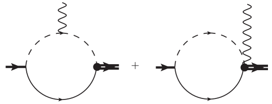
Figure 2: The diagrams contributing to the irreducible vertex that determines the $S$-to-$D$ state transition in Halo EFT. The thick double line denotes the dressed $D$-wave propagator and the thick single line the dressed $S$-wave propagator.

The diagrams contributing to the irreducible vertex for the E2 transition from the $S$- to the $D$-wave state at LO are shown in Fig. 2. At higher order, the next contribution would be the counterterm $L_{E2}^{(sd)}$ from Eq. (27) which has to be fixed by experimental input. The interaction term proportional to $L_{E2}^{(sd)}$ is not required to cancel any divergence because the LO contributions to the B(E2) transition depicted in Fig. 2 are finite. Therefore, our minimal principle of including the counterterms when they are needed for renormalization cannot be used to determine its exact order beyond LO. Thus, we restrict ourselves to LO for the reduced E2 transition strength. This allows us to make predictions for other electric observables as discussed below.

The photon in Fig. 2 has a four momentum of $k=(\omega,\mathbf{k})$ and its polarization index is denoted by $\nu$. The computation of the relevant diagrams yields a vertex function $\Gamma_{m^{\prime}m_{s}\nu}$, where $m^{\prime}$ is the total angular momentum projection of the $D$-wave state and $m_{s}$ denotes the spin projection of the $S$-wave state. Since the neutron spin is unaffected by this transition, we calculate the vertex function with respect to the specific components of the $D$-wave interaction

$$\Gamma_{m^{\prime}m_{s}\nu}=\sum_{m_{l}}\left(\left.\frac{1}{2}m_{s}\ 2m_{l}\right|Jm^{\prime}\right)\sum_{\alpha\beta}\left(\left.1\alpha\ 1\beta\right|2m_{l}\right)\tilde{\Gamma}_{\alpha\beta\nu}\ ,$$ (28)

where $J$ denotes the total spin of the $D$-wave state. In the case of $m_{s}=m^{\prime}=\pm 1/2$, only $m_{l}=0$ contributes to the sum in Eq. (28) and we get for $J=5/2$

$$\Gamma_{+\frac{1}{2}\,+\frac{1}{2}\,\nu}=\Gamma_{-\frac{1}{2}\,-\frac{1}{2}\,\nu}=\sqrt{\frac{2}{5}}\tilde{\Gamma}_{00\nu}\ +\sqrt{\frac{1}{10}}\tilde{\Gamma}_{1-1\nu}+\sqrt{\frac{1}{10}}\tilde{\Gamma}_{-11\nu}\ .$$ (29)

We calculate the irreducible vertex in Coulomb gauge so that we have $\mathbf{k}\cdot\mathbf{\epsilon}=0$ for real photons. In order to isolate the electric contribution to the irreducible vertex in a simple way, we choose $\mathbf{k}\cdot\mathbf{p}=0$, where $\mathbf{p}$ denotes the incoming momentum of the $S$-wave state. Taking gauge invariance and symmetry properties into account, the space-space components of the vertex function in Cartesian coordinates can be written as

$$\tilde{\Gamma}_{ijk}=\Gamma_{E}\ \frac{1}{2}\left(k_{j}\delta_{ik}+k_{i}\delta_{jk}\right)\ +\ \Gamma_{M}\ p_{k}\left(k_{i}k_{j}\ -\frac{1}{3}\delta_{ij}k^{2}\right).$$ (30)

Choosing the photon to be traveling in the $x_{3}$ direction only $\Gamma_{E}$ contributes to $\tilde{\Gamma}_{333}$, and we obtain

$$\tilde{\Gamma}_{333}=\Gamma_{E}\omega\ ,$$ (31)

with $|\mathbf{k}|=k_{3}=\omega$. By comparing the definitions for the transition rate depending on B(E2) and the transition rate as a function of the irreducible vertex $\Gamma_{E}$ Greiner et al. (1996), we get the following relation

B(E2: $$1/2^{+}\rightarrow 5/2^{+} =\frac{15}{\pi}\ \left(\frac{\Gamma_{+\frac{1}{2}\,+\frac{1}{2}\,0}}{\omega^{2}}\right)^{2}\ .$$)

Evaluating this using Eqs. (29, 31), it follows that $\Gamma_{+\frac{1}{2}\,+\frac{1}{2}\,0}=\sqrt{2/5}\;\tilde{\Gamma}_{333}$ and we obtain

B(E2: $$1/2^{+}\rightarrow 5/2^{+} =\ \frac{6}{\pi}\ \left(\frac{\bar{\Gamma}_{E}}{\omega}\right)^{2}\ ,$$)

with the renormalized, irreducible vertex $\bar{\Gamma}_{E}=\sqrt{Z_{\sigma}Z_{d}}\,\Gamma_{E}$. At LO, $Z_{\sigma}$ and $Z_{d}$ are given in Eqs. (65) and (19), respectively. Using the result of our calculation of $\Gamma_{E}$ for diagrams (a), we find at LO

B(E2: $$1/2^{+}\to 5/2^{+} =\frac{4}{5\pi}\frac{Z_{\text{eff}}^{2}e^{2}\gamma_{0}}{-r_{2}-\mathcal{P}_{2}\gamma_{2}^{2}}\ \left[\frac{3\gamma_{0}^{2}+9\gamma_{0}\gamma_{2}+8\gamma_{2}^{2}}{(\gamma_{0}+\gamma_{2})^{3}}\right]^{2},$$) (32)

where $\gamma_{2}$, $r_{2}$, and $\mathcal{P}_{2}$ are the parameters of the $5/2^{+}$ state and the effective charge is $Z_{\text{eff}}=(m_{n}/M_{nc})^{2}Q_{c}$. In general, the effective charge for arbitrary multipolarity $\lambda$ is given by $Z_{\text{eff}}^{(\lambda)}=Z_{n}\left(\frac{M}{M_{nc}}\right)^{\lambda}+Z_{c}\left(-\frac{m_{n}}{M_{nc}}\right)^{\lambda}$  Typel and Baur (2005). In Halo EFT it comes automatically out of the calculation.

The same result for $\bar{\Gamma}_{E}$ can be obtained using current conservation,

$$\omega\tilde{\Gamma}_{ij0}=k_{k}\tilde{\Gamma}_{ijk}\ ,$$ (33)

if we calculate the space-time components of the vertex function $\tilde{\Gamma}$. In contrast to $\tilde{\Gamma}_{ijk}$, we have to consider only the left diagram in Fig. 2 for $\tilde{\Gamma}_{ij0}$ at LO.

The calculation of the transition to the $3/2^{+}$ state can be carried out in the same way. The only difference is a relative factor of $2/3$ for B(E2) because of the different Clebsch-Gordan coefficient in Eq. (29)

B(E2: $$1/2^{+}\to 3/2^{+} =\frac{8}{15\pi}\frac{Z_{\text{eff}}^{2}e^{2}\gamma_{0}}{-r_{2}-\mathcal{P}_{2}\gamma_{2}^{2}}\ \left[\frac{3\gamma_{0}^{2}+9\gamma_{0}\gamma_{2}+8\gamma_{2}^{2}}{(\gamma_{0}+\gamma_{2})^{3}}\right]^{2},$$) (34)

where $\gamma_{2}$, $r_{2}$, and $\mathcal{P}_{2}$ are now the parameters of the $3/2^{+}$ state.

III.3 Form factors

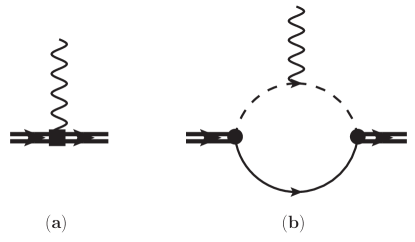
Figure 3: The topologies contributing to the irreducible vertex for an $A_{0}$ photon coupling to the ¹⁴C-neutron $D$-wave bound state up to NLO. Diagram (a) contains three different direct couplings. Two arise from minimal substitution in the bare propagator proportional to $r_{2}$, $\mathcal{P}_{2}$ and contribute at LO, while diagram (b) emerges from minimal substitution in the core propagator and contributes at NLO. The local gauge invariant operator $\sim L_{C01/2}^{(d)}$, required for the renormalization of diagram (b), is also represented by diagram (a) and contributes at NLO. The thick double line denotes the dressed $D$-wave propagator.

The result for the electric form factor of an $S$-wave halo state is discussed in Ref. Hammer and Phillips (2011) for ¹¹Be and in Ref. Fernando et al. (2015) for ¹⁵C. The experimental result for the rms charge radius of ¹⁴C is $\braket{r_{E}^{2}}^{1/2}_{{}^{14}\text{C}}=2.5025(87)$ fm Angeli and Marinova (2013) and the Halo EFT result for the $\frac{1}{2}^{+}$ $S$-wave ground state is $\braket{r_{E}^{2}}_{{}^{15}\text{C}}^{(\sigma)}\approx 0.11\ \text{fm}^{2}$ Fernando et al. (2015), but the authors do not quote an error for this number. In principle, both values can be combined to obtain a prediction for the full charge radius of the ¹⁵C ground state.

Here, we focus on the form factors of the $D$-wave state in ¹⁵C. The $D$-wave form factors can be extracted from the irreducible vertex for $A_{0}dd$ interactions. The corresponding contributions are shown in Fig. 3 up to NLO. The first diagram represents three different direct couplings of the photon to the $D$-wave propagator. Two couplings emerge from the minimal substitution in the bare propagator proportional to $r_{2}$, $\mathcal{P}_{2}$ and contribute at LO. The last one is a term $\sim L_{C01/2}^{(d)}$ which comes out of Eq. (27) and is required for the renormalization of the loop divergences of diagram (b) and therefore contributes at NLO. The second diagram arises from minimal substitution in the core propagator and contributes at NLO. The computation is carried out in the Breit frame, $q=(0,\mathbf{q})$, and the irreducible vertex for the $A_{0}$ photon coupling to the $D$-wave state in Cartesian coordinates yields

$$\Big{\langle}ij\left|J^{0}\right|op\Big{\rangle}= -ieQ_{c}\left[G_{E}(|\mathbf{q}|)\ E_{ij,op}+\frac{1}{2M_{nc}^{2}}G_{Q}(|\mathbf{q}|)\ Q_{ij,op}+\frac{1}{4M_{nc}^{4}}G_{H}(|\mathbf{q}|)\ H_{ij,op}\right]\ ,$$ (35)

with the three-momentum of the virtual photon $\mathbf{q}=\mathbf{p^{\prime}}-\mathbf{p}$ and three different $D$-wave tensors for each form factor $E_{ij,op}\sim q^{0}$, $Q_{ij,op}\sim q^{2}$ and $H_{ij,op}\sim q^{4}$. Note that we take out an overall factor of the elementary charge $e$ from all form factors. As a consequence our definition of the quadrupole and hexadecapole moments does not contain a factor $e$. Evidently, the hexadecapole form factor is only observable for the $5/2^{+}$ $D$-wave state and unobservable for the $3/2^{+}$ state. This can be straightforwardly proven by considering the respective Clebsch-Gordan coefficients to couple the spin and angular momentum to total $J$ for the two $D$-wave states in combination with $H_{ij,op}$ in spherical coordinates. For reasons of simplicity, the calculation is carried out in Cartesian coordinates and the resulting Cartesian tensors are given below

$$\tilde{Q}_{ij,op} =\frac{1}{4}\left(q_{j}q_{p}\delta_{io}+q_{j}q_{o}\delta_{ip}+q_{i}q_{p}\delta_{jo}+q_{i}q_{o}\delta_{jp}-\frac{4}{3}q_{i}q_{j}\delta_{op}-\frac{4}{3}q_{o}q_{p}\delta_{ij}+\frac{4}{9}q^{2}\delta_{ij}\delta_{op}\right)\ ,$$ (36)

$$\tilde{H}_{ij,op} =\left(q_{i}q_{j}q_{o}q_{p}-\frac{1}{3}q^{2}q_{i}q_{j}\delta_{op}-\frac{1}{3}q^{2}q_{o}q_{p}\delta_{ij}+\frac{1}{9}q^{4}\delta_{ij}\delta_{op}\right)\ ,$$ (37)

$$E_{ij,op} =\frac{\left(\delta_{io}\delta_{jp}+\delta_{ip}\delta_{jo}-\frac{2}{3}\delta_{ij}\delta_{op}\right)}{2}\ ,$$ (38)

$$Q_{ij,op} =\frac{3}{5}\tilde{Q}_{ij,op}-\frac{1}{5}q^{2}E_{ij,op}\ ,$$ (39)

$$H_{ij,op} =\frac{3}{2}\tilde{H}_{ij,op}-\frac{30}{35}q^{2}\tilde{Q}_{ij,op}+\frac{3}{35}q^{4}E_{ij,op}\ .$$ (40)

The Cartesian tensors $E_{ij,op}$, $Q_{ij,op}$ and $H_{ij,op}$ fulfill the following constraints

$$E_{ij,op}\ E_{ij,op}=5,\qquad\delta_{ij}\ E_{ij,op}=\delta_{op}\ E_{ij,op}=0\ ,$$ (41)

$$E_{ij,op}\ Q_{ij,op}=0,\qquad\delta_{ij}\ Q_{ij,op}=\delta_{op}\ Q_{ij,op}=0\ ,$$ (42)

$$E_{ij,op}\ H_{ij,op}=0,\qquad Q_{ij,op}\ H_{ij,op}=0,\qquad\delta_{ij}\ H_{ij,op}=\delta_{op}\ H_{ij,op}=0\ .$$ (43)

The neutron spin is unaffected by the charge operator up to the order considered here.

At LO, only the direct coupling from the minimal substitution in the bare $D$-wave propagator proportional to $r_{2}$ and $\mathcal{P}_{2}$, depicted in Fig. 3 (a), contribute. This reproduces the correct normalization condition of the electric form factor of $G_{E}(0)=1$, but the form factor is just a constant. Therefore, there is no real prediction beyond charge conservation at LO.

At NLO, diagram (b) in Fig. 3 also contributes, and the counterterm is required for the renormalization of the loop divergences stemming from diagram (b). We then obtain for the electric $G_{E}(|\mathbf{q}|)$, quadrupole $G_{Q}(|\mathbf{q}|)$ and hexadecapole $G_{H}(|\mathbf{q}|)$ form factors

$$G_{E}(|\mathbf{q}|)= \ \frac{1}{r_{2}+\mathcal{P}_{2}\gamma_{2}^{2}}\left[\left(\tilde{L}_{C01}^{(d)}+\frac{4}{3}\tilde{L}_{C02}^{(d)}\right)|\mathbf{q}|^{2}-\frac{21\gamma_{2}f^{2}|\mathbf{q}|^{2}}{16}+\frac{\gamma_{2}^{3}}{4}+\gamma_{2}^{2}\mathcal{P}_{2}+r_{2}\right.$$

$$\left.-\arctan\left(\frac{f|\mathbf{q}|}{2\gamma_{2}}\right)\left(\frac{21f^{3}|\mathbf{q}|^{3}}{32}+\frac{13\gamma_{2}^{2}f|\mathbf{q}|}{4}+\frac{\gamma_{2}^{4}}{2f|\mathbf{q}|}\right)\right],$$ (44)

$$G_{Q}(|\mathbf{q}|)= \ \frac{2M_{nc}^{2}}{r_{2}+\mathcal{P}_{2}\gamma_{2}^{2}}\left[\frac{20}{3}\tilde{L}_{C02}^{(d)}-\frac{75\gamma_{2}f^{2}}{14}-\frac{25\gamma_{2}^{3}}{7|\mathbf{q}|^{2}}\right.$$

$$\left.-\arctan\left(\frac{f|\mathbf{q}|}{2\gamma_{2}}\right)\left(\frac{75f^{3}|\mathbf{q}|}{28}+\frac{75\gamma_{2}^{2}f}{14|\mathbf{q}|}-\frac{50\gamma_{2}^{4}}{7f|\mathbf{q}|^{3}}\right)\right],$$ (45)

$$G_{H}(|\mathbf{q}|)= \ \frac{2}{3}\ \frac{4M_{nc}^{4}}{r_{2}+\mathcal{P}_{2}\gamma_{2}^{2}}\left[-\frac{45\gamma_{2}f^{2}}{64|\mathbf{q}|^{2}}+\frac{45\gamma_{2}^{3}}{16|\mathbf{q}|^{4}}\right.$$

$$\left.-\arctan\left(\frac{f|\mathbf{q}|}{2\gamma_{2}}\right)\left(\frac{45f^{3}}{128|\mathbf{q}|}-\frac{15\gamma_{2}^{2}f}{16|\mathbf{q}|^{3}}+\frac{45\gamma_{2}^{4}}{8f|\mathbf{q}|^{5}}\right)\right],$$ (46)

with $f=m_{R}/M$ while $\tilde{L}_{C01/2}^{(d)}$ represents the local gauge invariant operators from Eq. (27). These operators have a finite piece $L_{C01/2}^{(d)\text{ fin}}$ as well as a $\mu$-dependent part that cancels the renormalization scale dependence from the loop contribution. For a better readability, we have absorbed some prefactors in the definition of the counterterms and defined the low-energy constants

$$\tilde{L}_{C01}^{(d)} =\frac{15\pi}{eQ_{c}g_{2}^{2}m_{R}^{2}}L_{C01}^{(d)\text{ fin}}\ ,$$ (47)

$$\tilde{L}_{C02}^{(d)} =\frac{15\pi}{eQ_{c}g_{2}^{2}m_{R}^{2}}L_{C02}^{(d)\text{ fin}}\ ,$$ (48)

which are used in Eqs. (44, 45, 46). The remaining divergence emerging from the loop diagram in Fig. 3 is absorbed by $\mathcal{P}_{2}$ from the direct photon coupling in diagram (a). After the expansion of Eq. (44)

$$G_{E}(|\mathbf{q}|)\approx 1-\frac{1}{6}\braket{r_{E}^{2}}|\mathbf{q}|^{2}+\ldots\ ,$$ (49)

we obtain $G_{E}(0)=1$ and an electric radius

$$\braket{r_{E}^{2}}^{(d)}\ =\ -\frac{12\tilde{L}_{C01}^{(d)}+16\tilde{L}_{C02}^{(d)}-35\gamma_{2}f^{2}}{2\left(r_{2}+\mathcal{P}_{2}\gamma_{2}^{2}\right)}\ ,$$ (50)

such that the electric radius is not a prediction.

We expand Eq. (45) and (46)

$$\frac{1}{M_{nc}^{2}}G_{Q}(|\mathbf{q}|) \approx\mu_{Q}\left(1-\frac{1}{6}\braket{r_{Q}^{2}}|\mathbf{q}|^{2}+\ldots\right),$$ (51)

$$\frac{1}{M_{nc}^{4}}G_{H}(|\mathbf{q}|) \approx\mu_{H}\left(1-\frac{1}{6}\braket{r_{H}^{2}}|\mathbf{q}|^{2}+\ldots\right),$$ (52)

and find the respective multipole moments

$$\mu_{Q}^{(d)} =\frac{10\left(4\tilde{L}_{C02}^{(d)}-5\gamma_{2}f^{2}\right)}{3\left(r_{2}+\mathcal{P}_{2}\gamma_{2}^{2}\right)}\leavevmode\nobreak\ ,$$ (53)

$$\mu_{H}^{(d)} =-\frac{2f^{4}}{3\gamma_{2}\left(r_{2}+\mathcal{P}_{2}\gamma_{2}^{2}\right)}\ ,$$ (54)

where we find the hexadecapole moment $\mu_{H}^{(d)}$ as a prediction. The electric radius $\braket{r_{E}^{2}}^{(d)}$ and the quadrupole moment $\mu_{Q}^{(d)}$ are not predicted. They are used to fix the counterterms $L_{C02}^{(d)}$ and $L_{C01}^{(d)}$. The quadrupole and hexadecapole radii yield

$$\braket{r_{Q}^{2}}^{(d)} =\frac{27f^{4}}{7\gamma_{2}\left(4\tilde{L}_{C02}^{(d)}-5\gamma_{2}f^{2}\right)}\ ,$$ (55)

$$\braket{r_{H}^{2}}^{(d)} =\frac{9f^{2}}{14\gamma_{2}^{2}}\ ,$$ (56)

where the hexadecupole radius is predicted by Halo EFT and the quadrupole radius depends on the counterterm $L_{C02}^{(d)}$, fixed by the quadrupole moment. Thus, we can predict the quadrupole radius if the quadrupole moment is known.

Finally, we can reinsert the matching conditions, Eqs. (50, 53), into the results for the electric and quadrupole form factors, Eqs. (44, 45), in order to get expressions in terms of observables only.

III.4 Correlations between electric observables

Up to this point, all results are universal and not specific for ¹⁵C. In this section, we explore universal relations between different observables for shallow $D$-wave bound states predicted by Halo EFT. Moreover, we combine our Halo EFT results with data and ab initio results from the IT-NCSM Roth (2009) to predict electric properties of ¹⁵C. In a second step, the correlations obtained in Halo EFT are compared to the E2 correlation based on the rotational model by Bohr and Mottelson Bohr and Mottelson (1975).

We note that the quantification of theory uncertainties is important in any application of EFT to actual systems. In our discussion below, we will estimate the theory uncertainties from the size of the expansion parameter $R_{core}/R_{halo}$. More sophisticated estimates can be obtained from Bayesian statistics Furnstahl et al. (2015); Wesolowski et al. (2016); Griesshammer et al. (2016), but such an analysis is beyond the scope of this manuscript.

To make predictions, we use the experimental transition strength $\text{B(E2)}=0.44(1)$ W.u. Ajzenberg-Selove (1986) from the $5/2^{+}\rightarrow 1/2^{+}$ transition in ¹⁵C to determine the denominator of the $D$-wave renormalization constant at LO, i.e. the combination $r_{2}+\mathcal{P}_{2}\gamma_{2}^{2}$. Converting to physical units, we obtain the strength $\text{B(E2)}=2.90(7)\ e^{2}\text{fm}^{4}$ for the transition $1/2^{+}\rightarrow 5/2^{+}$. The experimental values of the binding momenta are $\gamma_{0}=0.235$ fm^-1 and $\gamma_{2}=0.147$ fm^-1 Ajzenberg-Selove (1986). Moreover, Fernando et al. Fernando et al. (2015) argued that it is more appropriate to count $r_{0}\sim\ R_{halo}$ for the specific case of ¹⁵C and thus we keep this contribution at LO in our application to ¹⁵C. The extracted value for $r_{0}=2.67\ \text{fm}$ Fernando et al. (2015) results from a fit to one-neutron capture data ¹⁴C$(n,\gamma){}^{15}$C Nakamura et al. (2009). With these data, we are able to determine the numerical value for $Z_{d}m_{R}^{2}g_{2}^{2}\sim 1/\left(r_{2}+\mathcal{P}_{2}\gamma_{2}^{2}\right)=-181(4)\ \text{fm}^{3}$.

Using our results from the previous sections, we obtain $\tilde{L}_{C01}^{(d)}+\frac{4}{3}\tilde{L}_{C02}^{(d)}=\braket{r_{E}^{2}}^{(d)}/1088(25)\ \text{fm}^{-1}$, $\tilde{L}_{C02}^{(d)}=-\mu_{Q}^{(d)}/2418(55)$ $\text{fm}^{-1}$ for the finite piece of the counterterms. For the hexadecapole moment and radius, we obtain the following predictions

$$\mu_{H}^{(d)}=1.68(4)(50)\times 10^{-2}\ \text{fm}^{4}\,,\ \mbox{ and }\ \braket{r_{H}^{2}}^{(d)}=0.135(3)(40)\ \text{fm}^{2}\,,$$ (57)

where the first uncertainty is due to the experimental input and the second one is a theory uncertainty from higher order corrections of order $R_{core}/R_{halo}\approx 0.3$ (see below).

Comparing our findings with Ref. Hammer and Phillips (2011) we find, as a general rule, that the highest multipole form factor is always independent of additional parameters from short-range counterterms. Moreover, we can always find a smooth correlation between the highest radius and the neutron separation energy $S_{n}$

$$\braket{r_{H}^{2}}^{(d)}=\frac{9}{28}\frac{f^{2}}{m_{R}S_{n}^{(d)}}\leavevmode\nobreak\ .$$ (58)

In the $S$- and $P$-wave case, we obtain

$$\braket{r_{Q}^{2}}^{(p)} =\frac{3}{10}\frac{f^{2}}{m_{R}S_{n}^{(p)}}\leavevmode\nobreak\ ,$$ (59)

$$\braket{r_{E}^{2}}^{(s)} =\frac{1}{4}\frac{f^{2}}{m_{R}S_{n}^{(s)}}\leavevmode\nobreak\ .$$ (60)

For the $D$-wave, we can derive several linear correlations between different combinations of multipole moments and radii. This is illustrated in Fig. 4, where the red cross denotes the numerical prediction of the corresponding quantity for ¹⁵C. Therefore, by measuring one of these observables, we can immediately predict the correlated quantity. These correlations are universal and can be found in arbitrary one-neutron $D$-wave halo nuclei or similar weakly-bound systems.

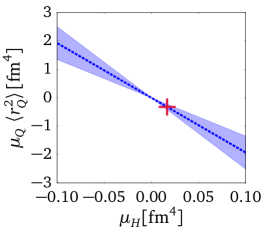
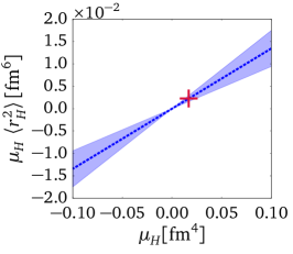
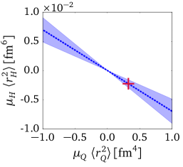
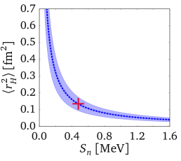
Figure 4: Linear correlations between the hexadecapole moment and the quadrupole moment times quadrupole radius (top left), the hexadecapole moment and the hexadecapole moment times hexadecapole radius (top right) and between the quadrupole moment times quadrupole radius and hexadecapole moment times hexadecapole radius (bottom left). Bottom right: correlation between the neutron separation energy and the hexadecapole radius. The red cross denotes the numerical prediction for ¹⁵C. The EFT uncertainties are given by the shaded bands.

With the numerical result for $Z_{d}m_{R}^{2}g_{2}^{2}$, we can check if our power counting scenario, leading to the scaling $Z_{d}m_{R}^{2}g_{2}^{2}\sim R_{halo}^{2}R_{core}$, can be confirmed or if the scenario of Bedaque et al. (2003) yields better agreement. An approximation for the halo scale can be extracted from the neutron separation energy $S_{n}$, $R_{halo}\approx 1/\gamma_{2}=1/\sqrt{S_{n}2m_{R}}=6.81\text{ fm}$. We can approximate the core scale by looking at the energy of the first excitation of the ¹⁴C nucleus $E_{ex}=6.1$ MeV. Converting this energy into a length scale, we obtain $R_{core}\approx 1.91$ fm. By employing the experimental values for $R_{halo}$ and $R_{core}$, we predict $Z_{d}m_{R}^{2}g_{2}^{2}\sim R_{halo}^{2}R_{core}\approx 90\text{ fm}^{3}$. This value is only by a factor of $2$ smaller than the one extracted from B(E2) and considering that this is an estimation grounded solely on the scaling within our power counting, our result is in reasonable agreement. The power counting of Bedaque et al. (2003) does lead to the scaling $Z_{d}m_{R}^{2}g_{2}^{2}=1/r_{2}\sim R_{core}^{3}\approx 7\text{ fm}^{3}$ which is around $26$ times smaller than the extracted result. These numbers indicate that our power counting scenario is better suited for ¹⁵C.

To obtain the correlation between the quadrupole transition from the $\frac{5}{2}^{+}$ to the $\frac{1}{2}^{+}$ state and the quadrupole moment of the $\frac{5}{2}^{+}$ state, we combine Eqs. (53) and (32) and apply a factor 2/6 to account for the different multiplicity of initial and final states. We obtain a linear dependence between B(E2) for the transition $\frac{5}{2}^{+}\to\frac{1}{2}^{+}$ and the quadrupole moment

$$\text{B(E2)}=\frac{-1}{50\pi}\ \frac{Z_{\text{eff}}^{2}\,e^{2}\gamma_{0}}{(1-r_{0}\gamma_{0})}\ \left[\frac{3\gamma_{0}^{2}+9\gamma_{0}\gamma_{2}+8\gamma_{2}^{2}}{(\gamma_{0}+\gamma_{2})^{3}}\right]^{2}\frac{\mu_{Q}^{(d)}}{\tilde{L}_{C02}^{(d)}-\frac{5}{4}\gamma_{2}f^{2}}\leavevmode\nobreak\ ,$$ (61)

where $\tilde{L}_{C02}^{(d)}$ is treated as fit parameter and $\gamma_{0}$ and $\gamma_{2}$ are taken from experiment Ajzenberg-Selove (1986).

A similar correlation between the quadrupole transition and the quadrupole moment can be obtained from the rotational model by Bohr and Mottelson Bohr and Mottelson (1975)

$$\text{B(E2},J_{i}\rightarrow J_{f}) =\frac{5}{16\pi}\frac{\left((J+1)(2J+3)\right)^{2}}{\left(3K^{2}-J(J+1)\right)^{2}}$$ (62)

$$\quad\times\left(\left.J_{i}K\ 20\right|J_{f}K\right)^{2}\left(\frac{Q^{0,t}}{Q^{0,s}}\right)^{2}\mu_{Q}(J)^{2}\ ,$$

where $K=1/2$ denotes the projection of the total angular momentum on the symmetry axis of the intrinsically deformed nucleus and $Q^{0,t}/Q^{0,s}$ is the ratio between intrinsic static ($s$) and transition ($t$) quadrupole moment in the rigid rotor model. The idea to employ this simple model is motivated by observations of Calci and Roth Calci and Roth (2016a), who found a robust correlation between this pair of quadrupole observables in ab initio calculations for light nuclei. In the simple rigid rotor model the ratio $Q^{0,t}/Q^{0,s}$ is expected to be one. The results of Ref. Calci and Roth (2016a) indicate that the correlation is robust as long as the ratio $Q^{0,t}/Q^{0,s}$ is treated as a fit parameter.

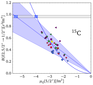
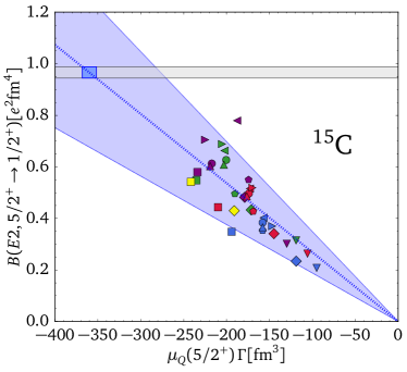
Figure 5: Correlation between B(E2) and the quadrupole moment $\mu_{Q}$. The IT-NCSM data is obtained with different NN+3N chiral EFT interactions: EM with cutoffs $\{400,400,500\}$ MeV/c (square, diamond, triangle down), and EGM with cutoffs $(\Lambda_{\chi}/\tilde{\Lambda}_{\chi})=\{(450/500),(600/500),(550/600),(450/700),(600/700)\}$ MeV/c (triangle left, pentagon, circle, triangle right, and triangle up) with oscillator frequency $\hbar\Omega=16$ MeV for all IT-NCSM calculations except for the diamond and triangle down data where $\hbar\Omega=20$ MeV. Different colors denote different $N_{\text{max}}=2$ (blue), 4 (red), 6 (green), 8 (violet), and 10 (yellow) values. Left panel: Rigid rotor model with quadratic fit of $Q^{0,t}/Q^{0,s}$ ratio (dashed line, $\chi_{red}^{2}=110$) and linear Halo EFT fit of $\tilde{L}_{C02}^{(d)}$ with fixed $\gamma_{2}$ from experiment (dotted line, $\chi_{red}^{2}=123$). Right panel: Linear Halo EFT fit with $\gamma_{0}^{2}-\gamma_{2}^{2}$ from IT-NCSM calculation and rescaled $\mu_{Q}/\Gamma$ (dotted line, $\chi_{red}^{2}=80$), where $\Gamma=\gamma_{0}(3\gamma_{0}^{2}+9\gamma_{0}\gamma_{2}+8\gamma_{2}^{2})^{2}/(1-r_{0}\gamma_{0})/(\gamma_{0}+\gamma_{2})^{6}$ divides out dependence on $\gamma_{0}$ and $\gamma_{2}$. The gray shaded area indicates the uncertainty band of the experimental B(E2) Ajzenberg-Selove (1986). The blue box within the gray shaded area corresponds to the prediction for $\mu_{Q}$. The EFT uncertainties are given by the blue shaded bands.

We use IT-NCSM data of ¹⁵C, generated by different chiral EFT interactions and different model spaces, to check the quadratic and linear correlations and predict numerically the quadrupole moment of ¹⁵C. This is demonstrated in Fig. 5. The varying symbols denote different NN+3N chiral EFT interactions which are similar to the ones used in Ref. Calci and Roth (2016a). We use the NN interaction developed by Entem and Machleidt (EM) Entem and Machleidt (2003) at N³LO with a cutoff of 500 MeV/c for the nonlocal regulator function. This NN force is combined with the local 3N force at N²LO using a cutoff of 400 or 500 MeV/c Navratil (2007). The second NN interaction by Epelbaum, Glöckle, Meißner (EGM) Epelbaum et al. (2004) at N²LO uses a nonlocal regularization with a cutoff $\Lambda_{\chi}$ and an additional spectral function regularization with cutoff $\tilde{\Lambda}_{\chi}$. The EGM NN forces are combined with a consistent nonlocal 3N force at N²LO used in several applications to neutron matter Hebeler and Furnstahl (2013); Tews et al. (2013); Krüger et al. (2013). For reasons of convergence, the NN+3N potentials are softened by a similarity renormalization group evolution where all contributions up to the three-body level are included.

We note that these interactions are based on Weinberg’s power counting Weinberg (1991) and their cutoff cannot be varied over a large range. However, chiral potentials based on Weinberg’s power counting have been very successful phenomenologically in nuclear structure and are currently the only potentials available that are well tested for p-shell nuclei. In particular, N²LO EGM interactions are still the only fully consistent set of two- and three-body interactions for which significant experience with structure calculations in the p-shell exists. Similarly, there is much experience with the EM interactions supplemented with (inconsistent) 3N forces. For this reason, we use these older interactions in our analysis. We believe that this is not a limiting factor of our analysis. After all, we are interested in universal properties which must emerge from any interaction that has the correct low-energy physics.

The different colors in Fig. 5 denote different $N_{\text{max}}$ values. The EFT uncertainties for the linear correlation are given by the blue shaded bands. Since the IT-NCSM results are not fully converged and the results differ for different $N_{\text{max}}$ values, the ordering of the ground and first excited state is exchanged for some data points. Leaving out the data sets with exchanged ordering does not significantly improve the fit. The plot on the left side employs the experimental values for the neutron separation energy as input for $\gamma_{0}$ and $\gamma_{2}$. For the plot on the right side, we use the excitation energy of the first excited state from the IT-NCSM to determine $\gamma_{0}^{2}-\gamma_{2}^{2}$ and for $\gamma_{0}$ we use the experimental value.

We emphasize that in the ab initio calculations, both, the interactions (including short distance physics) and the model spaces are varied. If the ab initio calculations were (i) fully converged and (ii) all interactions and electric operators were unitarily equivalent at the $A$-body level, they would fall on a single point. However, neither (i) nor (ii) is the case here. So, naively, one would expect the calculations for B(E2) and $\mu_{Q}$ to fill the whole plane. Halo EFT and the rotational model, however, predict a one parameter correlation between B(E2) and $\mu_{Q}$ based on certain assumptions. If these assumptions, such as shallow binding and a corresponding separation of scales in the case of Halo EFT, are satisfied in the ab initio calculations, they should also show the correlation even if they are not converged and/or have different short distance physics. A similar behavior is observed in the case of the Phillips and Tjon line correlations in light nuclei which are also satisfied by ”unphysical” calculations (See, e.g., Ref. Nogga et al. (2004) for an explicit example).

An additional complication here is the appearance of the two-body coupling $L_{C02}^{(d)}$ in Eq. (27) which could vary for the different ab initio data sets. In our analysis of the ab initio data, we explicitly assume that $L_{C02}^{(d)}$ varies only slowly and can be approximated by a constant for the ab initio data considered. Under this assumption, it becomes possible to decide between the type of correlation using the ab initio data for ¹⁵C.

From the left plot, we obtain $\mu_{Q}^{(d)}\approx-3.98(5)$ fm² for the quadratic fit and $\mu_{Q}^{(d)}\approx-5.46(12)(1.64)$ fm² for the linear fit, where the uncertainties from B(E2) are given in parenthesis. The second uncertainty for the linear fit is from higher orders in the EFT. From the fits, we cannot decide which scenario describes the IT-NCSM data more appropriately since both lead to similar reduced $\chi^{2}$ values of $\chi_{red}^{2}=110$ for the quadratic fit and $\chi_{red}^{2}=123$ for the linear fit. Please note that the absolute $\chi_{red}^{2}$ values have no significance since the theoretical errors of the ab initio results were not included in the fit, and only a relative comparison makes sense. The ratio $Q^{0,t}/Q^{0,s}$ should be equal to $1$ for an ideal rigid rotor. Since the quadratic fit yields a ratio of $Q^{0,t}/Q^{0,s}\approx 0.5$, we assume that ¹⁵C is not a good example of a rigid rotor. Perhaps for larger $N_{\text{max}}$ values, and thus better converged results, the matching between fit curves and data points would improve.

In the linear case, the slope of the fit depends also on the neutron separation energies of both states, which differ for each data point from the IT-NCSM. From the excitation energy obtained in the IT-NCSM calculation, we only know the difference between the neutron separation energies of the ground and excited state. Thus, one experimental input is still required to fix $\gamma_{0}$ and $\gamma_{2}$ from the IT-NCSM data, since we did not perform explicit calculations for ¹⁴C. In the right plot of Fig. 5, we determine $\gamma_{0}^{2}-\gamma_{2}^{2}$ from IT-NCSM data and take $\gamma_{0}$ from experiment. We deem this analysis to be more consistent than the previous one. The reduced $\chi^{2}$ value for the linear fit then slightly improves to $\chi_{red}^{2}=80$ compared to the fit using experimental values only. This leads to $\mu_{Q}^{(d)}\approx-4.21(10)(1.26)\ \mathrm{fm}^{2}$, which is closer to the value from the quadratic fit. The deviations of the data points from the linear fit might decrease further if consistent values for both neutron separation energies were extracted from the IT-NCSM. This NLO correlation is expected to hold up to corrections of order $R_{core}/R_{halo}\approx 0.3$ given by the blue shaded band. Taking this EFT uncertainty into account, the ab initio data satisfy the correlation very well.

With the extracted results of $\mu_{Q}^{(d)}$, we can predict the quadrupole radius, $\braket{r_{Q}^{2}}^{(d)}=5.93(13)(1.78)$ $\times$ $10^{-2}$ fm² from the left linear fit and $\braket{r_{Q}^{2}}^{(d)}=7.70(17)(2.31)\times 10^{-2}$ fm² from the right linear fit in Fig. 5, by Halo EFT.

Finally, we note that the NCSM calculations for small $N_{max}$ are not converged in the IR. However, it can be clearly seen in Fig. 5 that our conclusions are unchanged if the smallest $N_{max}=2,4,6$ are omitted. In fact, Calci et al. Calci and Roth (2016b) showed explicitly that the universal correlation between the B(E2: $0^{+}\to 2^{+}$) and the quadrupole moment of the $2^{+}$ state in ¹²C is extremely well satisfied even for the smallest $N_{max}$.

IV Conclusion

We have extended the Halo EFT approach for electric observables to shallow $D$-wave bound states. Additionally, a basic framework for the extension of our Halo EFT to higher partial waves has been outlined. We have developed a power counting scheme for arbitrary $l$-th partial wave shallow bound states that differs from the scenario of Bedaque et al. (2003) for $l>1$. This power counting was applied to ¹⁷C in Ref. Braun et al. (2018) where also some magnetic observables were considered. For higher partial waves the number of fine-tuned parameters increases. Based on the assumption that a larger number of fine tunings is less natural, this suggests that shallow bound states in higher partial waves are less likely than in lower ones, which is also observed experimentally.

Using this scheme, we have computed the B(E2) strength at LO and found that no additional counterterm is required at this order. We have also calculated the electric quadrupole as well as hexadecapole form factors at NLO and found a smooth, universal correlation between the quadrupole radius and the hexadecapole moment. We find that for the $D$-wave, the local gauge invariant operators become more important than in lower partial waves and counterterms are required for the form factors already at NLO. This continues the trend, observed in Hammer and Phillips (2011), that the counterterms enter in lower orders at larger $l$. The emergence of counterterms in low orders limits the predictive power of Halo EFT for $D$-waves. However, this limitation can be overcome by considering universal correlations between observables as discussed below.

We emphasize that, up to this point, all our results are universal and not specific for ¹⁵C. Considering now ¹⁵C as an example, the lack of data for the first excited $\frac{5}{2}^{+}$ state makes numerical predictions difficult. Using our result for the B(E2) and by comparing it to the measured B(E2) data, we have been able to make predictions for the hexadecapole moment $\mu_{H}^{(d)}=1.68(4)(50)\times 10^{-2}\ \text{fm}^{4}$ and radius $\braket{r_{H}^{2}}^{(d)}=0.135(3)(40)\ \text{fm}^{2}$. We cannot directly predict values for the charge radius and quadrupole moment and radius at NLO since the expressions (50), (53) and (55) contain unknown counterterms. Nevertheless, we have determined a value for the quadrupole moment, $\mu_{Q}^{(d)}\approx-4.21(10)(1.26)\ \mathrm{fm}^{2}$, by exploiting the linear correlation between the reduced E2 transition strength B(E2) and the quadrupole moment in our Halo EFT and fitting the unknown counterterm to ab initio results from the IT-NCSM. For consistency reasons, we prefer the result from the right plot of Fig. 5 using the excitation energy from IT-NCSM calculation. With this result for the quadrupole moment, we have also predicted the quadrupole radius for ¹⁵C, $\braket{r_{Q}^{2}}^{(d)}\approx 7.70(17)(2.31)\times 10^{-2}\ \mathrm{fm}^{2}$, using universal correlations from Halo EFT. These correlations are not obvious in ab initio approaches, since the separation of scales is not explicit in the parameters of the theory. This demonstrates the complementary character of Halo EFT towards ab initio methods. In principle, the universal correlations allow to extract information even from unconverged ab initio calculations since the correlations are universal. We have compared the linear Halo EFT correlation to the quadratic correlation based on the simple rotational model by Bohr and Mottelson. The value for the quadrupole moment, $\mu_{Q}^{(d)}\approx-3.98(5)\ \mathrm{fm}^{2}$, obtained from the quadratic correlation deviates from the linear result by 5% – 30% depending on the input used for $\gamma_{0}^{2}-\gamma_{2}^{2}$.

While there is a clear correlation in the ab initio data, there are also some outliers. In the case of the linear Halo EFT correlation, this could be due to the use of the experimental value of the ground state neutron separation energy $\gamma_{0}$, which is presumably inconsistent with some of the ab initio data sets. Since the Halo EFT correlation depends on the exact neutron separation energy of the two states, consistent values should be used. However, within the EFT uncertainty the predicted correlation is well satisfied. Better converged data sets and the future determination of the neutron separation energy directly from the IT-NCSM would help to clarify the situation. This proves the usefulness of our Halo EFT approach even for $D$-wave bound states, but also demonstrates the limiting factors for the extension to higher partial waves.

Appendix A S-wave propagator

The dressed $\sigma$ propagator and the $S$-wave scattering amplitude are computed by summing the bubble diagrams analog to the $D$-wave case shown in Fig. 1. The result for the dressed $\sigma$ propagator is

$$D_{\sigma}(p) =\frac{1}{\Delta_{0}+\eta_{0}[p_{0}-\mathbf{p}^{2}/(2M_{nc})+i\epsilon]-\Sigma_{\sigma}(p)}\leavevmode\nobreak\ ,$$ (63)

$$\Sigma_{\sigma}(p) =-\frac{g^{2}_{0}m_{R}}{2\pi}\left[i\sqrt{2m_{R}\left(p_{0}-\frac{\mathbf{p}^{2}}{2M_{nc}}\right)}+\mu\right]\leavevmode\nobreak\ ,$$ (64)

where PDS is employed as regularization scheme with scale $\mu$ Kaplan et al. (1998a, b). After matching to the effective range expansion, we obtain for the $\sigma$ propagator

$$D_{\sigma}(p) =Z_{\sigma}\frac{1}{p_{0}-\frac{\mathbf{p}^{2}}{2M_{nc}}+B_{0}}+R_{\sigma}(p)\ ,$$

with

$$Z_{\sigma}=\frac{2\pi\gamma_{0}}{m_{R}^{2}g_{0}^{2}}\quad\mbox{(LO)}\ ,\quad Z_{\sigma}=\frac{2\pi}{m_{R}^{2}g_{0}^{2}}\gamma_{0}\left[1+\gamma_{0}r_{0}\right]\quad\mbox{(NLO)}\ .$$ (65)

Here, $Z_{\sigma}$ denotes the wave-function renormalization, $B_{0}=\gamma_{0}^{2}/(2m_{R})$ denotes the binding energy and the remainder $R_{\sigma}(p)$ is regular at the pole.

References

- Jensen et al. (2004) A. S. Jensen, K. Riisager, D. V. Fedorov, and E. Garrido, Rev. Mod. Phys. 76, 215 (2004).
- Riisager (2013) K. Riisager, Phys. Scripta T152, 014001 (2013), arXiv:1208.6415 [nucl-ex] .
- Bertulani et al. (2002) C. A. Bertulani, H.-W. Hammer, and U. Van Kolck, Nucl. Phys. A712, 37 (2002), arXiv:nucl-th/0205063 [nucl-th] .
- Bedaque et al. (2003) P. F. Bedaque, H.-W. Hammer, and U. van Kolck, Phys. Lett. B569, 159 (2003), arXiv:nucl-th/0304007 [nucl-th] .
- Ando (2016) S.-I. Ando, Int. J. Mod. Phys. E25, 1641005 (2016), arXiv:1512.07674 [nucl-th] .
- Rupak (2016) G. Rupak, Int. J. Mod. Phys. E25, 1641004 (2016).
- Hammer et al. (2017) H.-W. Hammer, C. Ji, and D. R. Phillips, J. Phys. G44, 103002 (2017), arXiv:1702.08605 [nucl-th] .
- Higa et al. (2008) R. Higa, H.-W. Hammer, and U. van Kolck, Nucl. Phys. A809, 171 (2008), arXiv:0802.3426 [nucl-th] .
- Canham and Hammer (2008) D. L. Canham and H.-W. Hammer, Eur. Phys. J. A37, 367 (2008), arXiv:0807.3258 [nucl-th] .
- Canham and Hammer (2010) D. L. Canham and H.-W. Hammer, Nucl. Phys. A836, 275 (2010), arXiv:0911.3238 [nucl-th] .
- Rotureau and van Kolck (2013) J. Rotureau and U. van Kolck, Few Body Syst. 54, 725 (2013), arXiv:1201.3351 [nucl-th] .
- Ji et al. (2014) C. Ji, C. Elster, and D. R. Phillips, Phys. Rev. C90, 044004 (2014), arXiv:1405.2394 [nucl-th] .
- Hammer and Phillips (2011) H.-W. Hammer and D. R. Phillips, Nucl. Phys. A865, 17 (2011), arXiv:1103.1087 [nucl-th] .
- Fernando et al. (2015) L. Fernando, A. Vaghani, and G. Rupak, (2015), arXiv:1511.04054 [nucl-th] .
- Rupak and Higa (2011) G. Rupak and R. Higa, Phys. Rev. Lett. 106, 222501 (2011), arXiv:1101.0207 [nucl-th] .
- Zhang et al. (2014a) X. Zhang, K. M. Nollett, and D. R. Phillips, Phys. Rev. C89, 024613 (2014a), arXiv:1311.6822 [nucl-th] .
- Rupak et al. (2012) G. Rupak, L. Fernando, and A. Vaghani, Phys. Rev. C86, 044608 (2012), arXiv:1204.4408 [nucl-th] .
- Acharya and Phillips (2013) B. Acharya and D. R. Phillips, Nucl. Phys. A913, 103 (2013), arXiv:1302.4762 [nucl-th] .
- Braun et al. (2018) J. Braun, H.-W. Hammer, and L. Platter, Eur. Phys. J. A54, 196 (2018), arXiv:1806.01112 [nucl-th] .
- Hagen et al. (2013) P. Hagen, H.-W. Hammer, and L. Platter, Eur. Phys. J. A49, 118 (2013), arXiv:1304.6516 [nucl-th] .
- Zhang et al. (2014b) X. Zhang, K. M. Nollett, and D. R. Phillips, Phys. Rev. C89, 051602 (2014b), arXiv:1401.4482 [nucl-th] .
- Brown and Hale (2014) L. S. Brown and G. M. Hale, Phys. Rev. C89, 014622 (2014), arXiv:1308.0347 [nucl-th] .
- Kaplan et al. (1998a) D. B. Kaplan, M. J. Savage, and M. B. Wise, Phys. Lett. B424, 390 (1998a), arXiv:nucl-th/9801034 [nucl-th] .
- Kaplan et al. (1998b) D. B. Kaplan, M. J. Savage, and M. B. Wise, Nucl. Phys. B534, 329 (1998b), arXiv:nucl-th/9802075 [nucl-th] .
- Ajzenberg-Selove (1986) F. Ajzenberg-Selove, Nucl. Phys. A449, 1 (1986).
- Roth (2009) R. Roth, Phys. Rev. C79, 064324 (2009), arXiv:0903.4605 [nucl-th] .
- Calci and Roth (2016a) A. Calci and R. Roth, Phys. Rev. C94, 014322 (2016a), arXiv:1601.07209 [nucl-th] .
- Bohr and Mottelson (1975) A. Bohr and B. R. Mottelson, Nuclear structure, vol. II (Benjamin, New York, 1975).
- Griesshammer (2004) H. W. Griesshammer, Nucl. Phys. A744, 192 (2004), arXiv:nucl-th/0404073 [nucl-th] .
- Tanabashi et al. (2018) M. Tanabashi et al. (Particle Data Group), Phys. Rev. D98, 030001 (2018).
- Beane and Savage (2001) S. R. Beane and M. J. Savage, Nucl. Phys. A694, 511 (2001), arXiv:nucl-th/0011067 [nucl-th] .
- van Kolck (1997) U. van Kolck, Chiral dynamics: Theory and experiment. Proceedings, Workshop, Mainz, Germany, September 1-5, 1997, (1997), 10.1007/BFb0104898, [Lect. Notes Phys.513,62(1998)], arXiv:hep-ph/9711222 [hep-ph] .
- van Kolck (1999) U. van Kolck, Nucl. Phys. A645, 273 (1999), arXiv:nucl-th/9808007 [nucl-th] .
- Buckingham (1959) A. Buckingham, Quarterly Reviews, Chemical Society 13, 183 (1959).
- Briceno et al. (2013) R. A. Briceno, Z. Davoudi, and T. C. Luu, Phys. Rev. D88, 034502 (2013), arXiv:1305.4903 [hep-lat] .
- Greiner et al. (1996) W. Greiner, D. A. Bromley, and J. Maruhn, Nuclear Models (Springer Berlin Heidelberg, 1996).
- Typel and Baur (2005) S. Typel and G. Baur, Nucl. Phys. A759, 247 (2005), arXiv:nucl-th/0411069 [nucl-th] .
- Angeli and Marinova (2013) I. Angeli and K. P. Marinova, Atom. Data Nucl. Data Tabl. 99, 69 (2013).
- Furnstahl et al. (2015) R. J. Furnstahl, N. Klco, D. R. Phillips, and S. Wesolowski, Phys. Rev. C92, 024005 (2015), arXiv:1506.01343 [nucl-th] .
- Wesolowski et al. (2016) S. Wesolowski, N. Klco, R. J. Furnstahl, D. R. Phillips, and A. Thapaliya, J. Phys. G43, 074001 (2016), arXiv:1511.03618 [nucl-th] .
- Griesshammer et al. (2016) H. W. Griesshammer, J. A. McGovern, and D. R. Phillips, Eur. Phys. J. A52, 139 (2016), arXiv:1511.01952 [nucl-th] .
- Nakamura et al. (2009) T. Nakamura et al., Phys. Rev. C79, 035805 (2009).
- Entem and Machleidt (2003) D. R. Entem and R. Machleidt, Phys. Rev. C68, 041001 (2003), arXiv:nucl-th/0304018 [nucl-th] .
- Navratil (2007) P. Navratil, Few Body Syst. 41, 117 (2007), arXiv:0707.4680 [nucl-th] .
- Epelbaum et al. (2004) E. Epelbaum, W. Gloeckle, and U.-G. Meißner, Eur. Phys. J. A19, 125 (2004), arXiv:nucl-th/0304037 [nucl-th] .
- Hebeler and Furnstahl (2013) K. Hebeler and R. J. Furnstahl, Phys. Rev. C87, 031302 (2013), arXiv:1301.7467 [nucl-th] .
- Tews et al. (2013) I. Tews, T. Krüger, K. Hebeler, and A. Schwenk, Phys. Rev. Lett. 110, 032504 (2013), arXiv:1206.0025 [nucl-th] .
- Krüger et al. (2013) T. Krüger, I. Tews, K. Hebeler, and A. Schwenk, Phys. Rev. C88, 025802 (2013), arXiv:1304.2212 [nucl-th] .
- Weinberg (1991) S. Weinberg, Nucl. Phys. B363, 3 (1991).
- Nogga et al. (2004) A. Nogga, S. K. Bogner, and A. Schwenk, Phys. Rev. C70, 061002 (2004), arXiv:nucl-th/0405016 [nucl-th] .
- Braaten and Hammer (2006) E. Braaten and H.-W. Hammer, Phys. Rept. 428, 259 (2006), arXiv:cond-mat/0410417 [cond-mat] .
- Calci and Roth (2016b) A. Calci and R. Roth, Phys. Rev. C94, 014322 (2016b), arXiv:1601.07209 [nucl-th] .