Revisit of cosmic ray antiprotons from dark matter annihilation with updated constraints on the background model from AMS-02 and collider data

Abstract

We study the cosmic ray antiprotons with updated constraints on the propagation, proton injection, and solar modulation parameters based on the newest AMS-02 data near the Earth and Voyager data in the local interstellar space, and on the cross section of antiproton production due to proton-proton collisions based on new collider data. We use a Bayesian approach to properly consider the uncertainties of the model predictions of both the background and the dark matter (DM) annihilation components of antiprotons. We find that including an extra component of antiprotons from the annihilation of DM particles into a pair of quarks can improve the fit to the AMS-02 antiproton data considerably. The favored mass of DM particles is about $60\sim 100$ GeV, and the annihilation cross section is just at the level of the thermal production of DM ($\langle\sigma v\rangle\sim O(10^{-26})$ cm³ s^-1).

1 Introduction

Cosmic ray (CR) antiprotons are one of the most important probes to indirectly detect dark matter (DM) particles. Quite a number of balloon and space detectors have been dedicated to precisely measuring the antiproton fluxes and antiproton-to-proton ratios since 1990s [1, 2, 3, 4, 5, 6, 7, 8, 9, 10, 11, 12, 13, 14]. Large progresses have been made in recent years thanks to the operation of the Payload for Antimatter Matter Exploration and Light-nuclei Astrophysics (PAMELA; [15]) and the Alpha Magnetic Spectrometer (AMS-02). The antiproton flux has been measured to $\sim 500$ GeV by AMS-02 with high precision [14], which improved the constraints on either the CR or the DM models effectively [16, 17, 18, 19, 20, 21, 22, 23, 24, 25].

The propagation of CRs is typically one of the largest sources of uncertainties in predicting the background of antiprotons and the signal from DM annihilation [26, 27, 28]. The propagation of charged particles in the Milky Way can be described by a diffusion process in the random magnetic field. The collision between primary nuclei and the interstellar gas leads to fragmentation of the parent nuclei and the production of secondary nuclei. Therefore the secondary-to-primary particle ratio, e.g., the Boron-to-Carbon (B/C) ratio, is usually employed to constrain the propagation parameters [29, 30, 31, 32]. The precise measurements of CR fluxes and/or flux ratios by AMS-02 [14, 33] shed new light on the understanding of CR propagation [16, 17, 34, 35, 36].

Using the improved constraints on the propagation model parameters [16, 34], it was found that there might be an excess of the antiproton flux around a few GeV energies compared with the background contribution from $pp$ collisions, and a DM model could simply explain this excess without constraints from other observations such as $\gamma$-rays [37, 38]. More interestingly, the model parameters to account for the antiproton excess are consistent with that proposed to explain the Galactic center $\gamma$-ray excess [39, 40, 41, 42], the tentative $\gamma$-ray excesses in the directions of two dwarf galaxies [43, 44], and a possible $\gamma$-ray line-like feature from a population of clusters of galaxies [45]. Such coincidence makes DM a promising explanation of the possible antiproton excess [46].

Most recently, the AMS-02 collaboration reported new measurements of the primary (He, C, O) and secondary (Li, Be, B) nucleus fluxes [47, 48]. These results are expected to give more consistent constraints on the CR propagation models and parameters since they are closely relevant parent and daughter particles (different from the B/C ratio and proton fluxes used in Ref. [34]). Using the Carbon flux and B/C ratio measured by AMS-02 [33, 47], together with the data at low energies by the Advanced Composition Explorer (ACE) spacecraft near the Earth and the Voyager in the local interstellar space [49, 50], Ref. [51] carried out a study of different propagation model settings and constrained the propagation parameters in a narrow region. In this work, we revisit the antiproton problem based on the new results of the CR propagation. The updated production cross section of antiprotons via $pp$ collisions with constraints from the most recent collider data will also be employed [52]. In addition, we also develop a more efficient method to calculate the likelihood of the DM component. In Section 2 we present the propagation and proton source parameters which are the basis of the calculation of the background antiproton flux. In Section 3 we investigate the DM contribution to antiprotons. We conclude our work in Section 4.

2 Propagation model parameters and background antiprotons

Charged particles propagate diffusively in a diffusive halo, usually assumed to feature cylindrical symmetry, with a radius of $R_{h}$ and a half-height $z_{h}$, defined by the extension of the magnetic field. The propagation equation can be written in general as

$$\frac{\partial\psi}{\partial t}=\nabla\cdot(D_{xx}\nabla\psi-{\bf V}\psi)+\frac{\partial}{\partial p}p^{2}D_{pp}\frac{\partial}{\partial p}\frac{\psi}{p^{2}}+\frac{\partial}{\partial p}\left[b\psi+\frac{p}{3}(\nabla\cdot{\bf V})\psi\right]-\frac{\psi}{\tau}+q.$$ (2.1)

The first term in the right-hand-side is the diffusion in the random magnetic field with $D_{xx}$ being the spatial diffusion coefficient, the second term represents the advection velocity which is assumed to linearly increase along the $z$-direction, the third term is the stochastic reacceleration characterized by a diffusion in the momentum space with a diffusion coefficient $D_{pp}$, the fourth and fifth terms are the interaction and adiabatic energy loss terms, the sixth term represents the fragmentation and/or decay, and the last term is the source function.

The diffusion coefficient is usually assumed to be spatially uniform in the Milky Way, and it can be parameterized as a power-law function of rigidity, $D(R)=\beta D_{0}(R/R_{0})^{\delta}$, where $\beta$ is the velocity of a particle (in unit of light speed), $D_{0}$ is a normalization constant, $\delta$ is the rigidity-dependence slope (see below for a modification of the diffusion coefficient). There are proposals of spatially non-uniform (e.g., [32, 53]) or anisotropic diffusion [54] scenarios motivated by recent observations of spectral hardenings of CRs [55, 56] and spatial variation of CR spectral indices inferred from Fermi-LAT $\gamma$-ray observations [57, 58]. It has been shown that the $\bar{p}/p$ ratio also hardens gradually at high energies in the spatially-dependent propagation model [32, 53], and may account for the flat behavior of the $\bar{p}/p$ ratio as observed by AMS-02 [14]. The effect on the low energy part of the antiproton spectrum (e.g., below 10 GeV) under such complicated propagation models needs further studies. Here we work under the simple uniform diffusion framework, which can actually explain most of the CR and diffuse $\gamma$-ray data.

The advection velocity is parameterized as ${\bf V}=dV/dz\cdot{\bf z}$. The reacceleration is characterized by the Alfvenic speed of the plasma, $v_{A}$, which bridges the spatial and momentum diffusion coefficients as $D_{pp}D_{xx}=\frac{4p^{2}v_{A}^{2}}{3\delta(4-\delta^{2})(4-\delta)}$ [59]. The momentum loss rate $b(p)=-\dot{p}$ includes the ionization and Coulomb scattering losses and radiative cooling (for electrons/positrons). The injection spectrum of nuclei is parameterized as a doubly broken power-law form of rigidity

$$q(R)\propto\left\{\begin{array}[]{ll}\left(R/R_{\mathrm{br},1}\right)^{-\nu_{1}},&R<R_{\mathrm{br,1}}\\ \left(R/R_{\mathrm{br},1}\right)^{-\nu_{2}},&R_{\mathrm{br,1}}\leq R<R_{\mathrm{br,2}}\\ \left(R/R_{\mathrm{br},1}\right)^{-\nu_{3}}\left(R_{\mathrm{br},2}/R_{\mathrm{br},1}\right)^{\nu_{3}-\nu_{2}},&R_{\mathrm{br,2}}\leq R\end{array},\right.$$ (2.2)

where $R_{\mathrm{br},1}\sim$ GV is to account for the low energy data, and $R_{\mathrm{br},2}\sim 300$ GV is to account for the high energy spectral hardening [55, 56].

We assume the force-field approximation to describe the solar modulation effect [60]. Since the time periods of data taking of protons and antiprotons by AMS-02 are slightly different, their modulation parameters should also be different. In this work we adopt $\Phi_{\bar{p}}=\Phi_{p}+0.02$ GV, as suggested by the time-dependent solar modulation potentials [34].

The numerical tool GALPROP [61, 62] is adopted to solve the propagation equation. It was found that the diffusion model with reacceleration of CRs by the random magnetohydrodynamic (MHD) waves fit the data better than the plain diffusion scenario and the model with a advective transportation [51]. In particular, a variant of the velocity-dependence of the diffusion coefficient, $D(R)=\beta^{\eta}D_{0}(R/R_{0})^{\delta}$, where $\eta$ is an empirical modification of the velocity-dependence [63], gives the best fit to the data [51]. Physically such a diffusion behavior may be related to the resonant interactions between CRs and the MHD waves which result in dissipations of such waves corresponding to low energy particles [64]. This model, referred to as DR2 hereafter, is employed to study antiprotons in this work.

We use the CosRayMC tool, which embeds the GALPROP code in the Markov Chain Monte Carlo driver, to fit the model parameters [65]. The proton fluxes measured by Voyager in the local interstellar space [50], AMS-02 [66], and CREAM [67] are used to derive the proton injection spectral parameters. We include the uncertainties of the propagation parameters from independent fit to the B/C ratio and Carbon fluxes as priors. See the Appendix for details of the prior information from the fitting covariance matrix. The fitting results of the source parameters are given in Table 1. Some of the propagation parameters, such as $D_{0}$ and $z_{h}$, are consistent with those derived previously in Ref. [34], while the others are slightly different. This is perhaps due to different data sets used in this work (in particular the inclusion of Voyager data). The propagation parameters can not be directly compared with that given in Ref. [38] due to different model settings. However, we find that the parameters $D_{0}$ and $z_{h}$ are still similar with each other. The best-fit results of the proton flux and the B/C ratio, together with the observational data, are shown in Figure 1. Note that the injection spectrum of Carbon nuclei is different from that of protons, and we use the results obtained in Ref. [51] to calculate the B/C ratio. The propagation parameters used to plot Figure 1 are the same as that in Table 1.

Table 1: Propagation and proton injection spectral parameters, together with their posterior $68\%$ errors, from fitting to the Voyager, AMS-02, and CREAM data.

Parameter	Unit	Value
$D_{0}^{\dagger}$	($10^{28}$cm2 s-1)	$5.98\pm 1.00$
$\delta$		$0.411\pm 0.008$
$z_{h}$	(kpc)	$5.58\pm 1.39$
$v_{A}$	(km s-1)	$27.5\pm 1.3$
$\eta$		$-0.27\pm 0.08$
$A_{p}^{\ddagger}$	($10^{-9}$ cm-2 s-1 sr-1)	$4.43\pm 0.01$
$\nu_{1}$		$2.03\pm 0.02$
$R_{\rm br,1}$	(GV)	$10.3\pm 0.9$
$\nu_{2}$		$2.40\pm 0.01$
$R_{\rm br,2}$	(GV)	$511.8\pm 86.2$
$\nu_{3}$		$2.25\pm 0.02$
$\Phi_{p}$	(GV)	$0.673\pm 0.015$

^†Normalization at $R_{0}=4$ GV. ^‡Normalization of the propagated proton flux at 100 GeV.

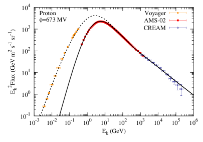
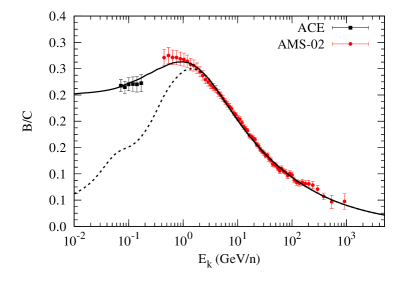
Figure 1: Best-fit proton flux (left) and B/C ratio (right) compared with the Voyager, AMS-02, and CREAM data. In each panel the dashed (solid) line is for the result before (after) the solar modulation.

The antiproton background produced by inelastic collisions between protons and the interstellar medium can be calculated using the same propagation, proton injection, and solar modulation parameters (referred to as background parameters hereafter) obtained through fitting to the proton flux data. The Markov chains of the background parameters are used, which include the correlations among different parameters. The cross section of antiproton production is an additional source of uncertainties [68, 69, 70, 71, 72, 52, 73]. In this work we employ the updated parameterization of the antiproton production cross section based on the most recent collider data [52]. The relative uncertainties of the antiproton fluxes are found to be $\lesssim 10\%$ in the relevant energy range covered by the AMS-02 data. Therefore we multiply a constant factor $\kappa$, which has a Gaussian prior of $N(1.0,0.1^{2})$ on the background antiproton flux when calculating its likelihood.

3 DM contribution to antiprotons

The same propagation parameters as obtained in Sec. II are adopted to calculate the antiproton flux from the DM annihilation. The source term of DM annihilation induced antiprotons can be written as

$$q_{\bar{p}}^{\rm DM}=\frac{\langle\sigma v\rangle}{2m_{\chi}^{2}}\frac{{\rm d}N}{{\rm d}E}\rho(\boldsymbol{x}),$$ (3.1)

where the DM particle is assumed to be Majorana fermion, $m_{\chi}$ is the mass of the DM particle, $\langle\sigma v\rangle$ is the velocity-weighted annihilation cross section, ${\rm d}N/{\rm d}E$ is the antiproton production spectrum per annihilation, and $\rho(\boldsymbol{x})$ is the density profile of DM which is assumed to be the Navarro-Frenk-White distribution [74]. The scale radius of the density profile is adopted to be 20 kpc, and the local density is assumed to be 0.3 GeV cm^-3 [75].

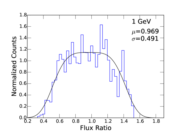
Figure 2: Distribution of ratios of the DM-induced antiproton fluxes for various background parameters $\boldsymbol{\theta}_{\rm bkg}$ to that calculated with the mean background parameters $\bar{\boldsymbol{\theta}}_{\rm bkg}$. The solid line is a fit using Eq. (3.2).

We adopt a simplified way to calculate the likelihood of the DM component taking into account the uncertainties of the background parameters. The antiproton fluxes from the DM annihilation span in a band when the background parameters change [37]. Figure 2 shows the distribution of the ratios of antiproton fluxes at 1 GeV to that calculated with the mean background parameters given in Table 1. This distribution can be fitted with a probability function

$$p(f)\propto\exp\left[-\left(\frac{f-\mu}{\sigma}\right)^{4}\right],$$ (3.2)

where $\mu=0.969$ and $\sigma=0.491$. The posterior probability of a given set of DM parameters, $(m_{\chi},\,\langle\sigma v\rangle)$, and specified annihilation channel(s), is

$$\mathcal{P}_{\rm DM}\propto\int\mathcal{L}_{\bar{p}}(\boldsymbol{\theta}_{\rm bkg},\kappa,f\bar{\phi}_{\rm DM})\,p(\boldsymbol{\theta}_{\rm bkg})\,p(\kappa)\,p(f)\,{\rm d}\boldsymbol{\theta}_{\rm bkg}\,{\rm d}\kappa\,{\rm d}f,$$ (3.3)

in which ${\mathcal{L}}_{\bar{p}}\propto\exp(-\chi^{2}_{\bar{p}}/2)$ is the likelihood of the model given the AMS-02 antiproton data, $\boldsymbol{\theta}_{\rm bkg}$ is the background parameters as listed in Table 1, $\kappa$ is a constant factor characterizing the uncertainties of the production cross section of antiprotons in $pp$ collisions, $\bar{\phi}_{\rm DM}$ is the flux of the DM component calculated with the mean background parameters $\bar{\boldsymbol{\theta}}_{\rm bkg}$, $f$ is a constant scale factor describing the variation of the fluxes due to the uncertainties of the background parameters, $p(\boldsymbol{\theta}_{\rm bkg})$, $p(\kappa)$, and $p(f)$ are the prior probabilities of these parameters, respectively. The prior distribution $p(\boldsymbol{\theta}_{\rm bkg})$ is obtained through fitting to the proton fluxes (Section 2). To avoid unphysical results with negative coefficients, we limit the prior regions of $f$ in $[0.2,1.8]$, and $\kappa$ in $[0.5,1.5]$ in the integration. We have tested that this approximation gives very similar results as the full computation as done in Ref. [37].

We find that a DM component is favored by the AMS-02 data. Assuming $b\bar{b}$ annihilation channel, the favored mass range of the DM particles is about $60\sim 100$ GeV, and the annihilation cross section is $(0.7\sim 7)\times 10^{-26}$ cm³ s^-1, as shown in Figure 3. We estimate the Bayes factor of a DM component with $b\bar{b}$ annihilation channel is about $8.4$, which can be regarded as strong evidence supporting the DM model. These results are consistent with that found previously [38, 37], although the Bayes factor is slightly smaller. The difference of the Bayes factor is due to the update of the propagation model and parameters with a more consistent treatment of the fit to the CR data, in particular the inclusion of the Voyager data. The favored parameter region of DM is also consistent with that inferred from the GeV $\gamma$-ray excess from the Galactic center (dashed contours; [41]). A large part of the favored parameter region lies below the constraints obtained with Fermi-LAT observations of a class of dwarf galaxies (dash-dotted line) [76]. A global fit to the data of antiprotons, and $\gamma$-rays from the Galactic center and dwarf galaxies give similar results [46], although the propagation model and parameters are different from ours. It can further be noted that such a cross section is also consistent with the value suggested by the relic density for the thermal production scenario of DM.

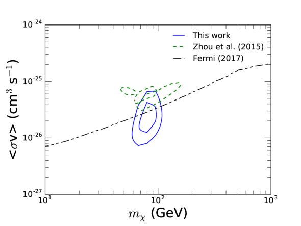
Figure 3: Favored $68\%$ and $95\%$ credible regions (solid contours) on the mass and annihilation cross section of DM for $b\bar{b}$ channel, compared with that inferred from the Galactic center $\gamma$-ray excess with a re-normalization of the local density (dashed contours; [41]). The $95\%$ exclusion limit of Fermi-LAT observations of dwarf galaxies is shown by the dash-dotted line [76].

Figure 4 illustrates the antiproton fluxes of the best-fit models, for the background-only hypothesis (left) and the background + DM hypothesis (right), respectively. Compared with the background prediction, excesses of antiprotons can be seen around a few GeV. It is interesting to note that at high energies the background model is quite consistent with the data, without any significant excess [23, 24, 22, 19, 25].

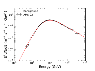
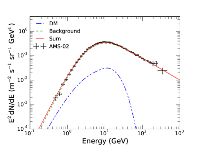
Figure 4: Best-fit model predictions of the antiproton fluxes, compared with the AMS-02 data. The left panel is for the background-only fit, and the right one is for the background + DM fit.

Finally we derive the upper limits on the DM annihilation cross section from the fit to the antiproton data. The $95\%$ upper limit for given $m_{\chi}$ is obtained from the following equation

$$\frac{\int_{0}^{\langle\sigma v\rangle_{95}}{\mathcal{P}}(x)\,{\rm d}x}{\int_{0}^{\infty}{\mathcal{P}}(x)\,{\rm d}x}=0.95.$$ (3.4)

The results are given in Figure 5. The limits are typically stronger than that obtained by $\gamma$-ray observations of dwarf galaxies, except for the “signal region” with $m_{\chi}\sim 50-130$ GeV. These limits may scale down by a constant factor, if the local density of DM is higher (e.g., [77, 78]).

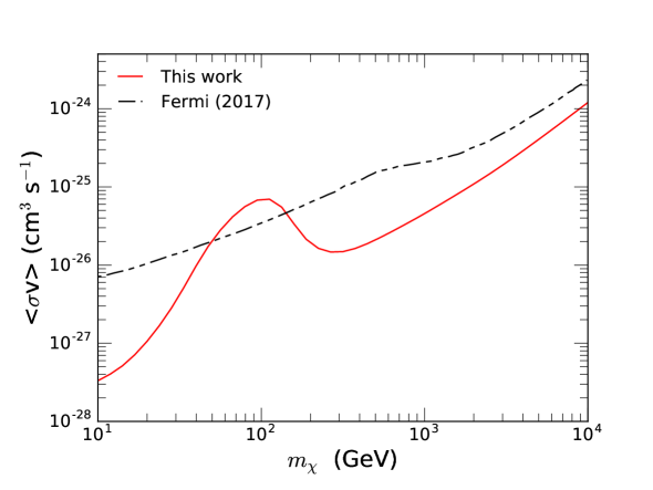
Figure 5: $95\%$ credible level upper limits of the annihilation cross section for $\chi\chi\to b\bar{b}$ obtained from AMS-02 antiproton data, and that from Fermi-LAT observations of dwarf galaxies [76].

4 Conclusion and discussion

In this work we revisit the indirect detection of DM with CR antiprotons. Several important updates are presented. The propagation parameters of CRs are obtained through fitting to the newest B/C and Carbon flux data by AMS-02, as well as the low energy observations near the Earth by ACE and in the local interstellar space by Voyager. Using the propagation parameters as priors, we fit the Voyager, AMS-02, and CREAM data of proton fluxes to obtain the source parameters of CR protons and the solar modulation potential. These newly obtained background parameters are then used to calculate the background antiproton fluxes. The production cross section of $pp$ collisions based on the recent collider data is employed. A Bayesian approach taking into account the uncertainties of the background parameters and antiproton production cross section is adopted.

We find that the AMS-02 antiproton data favor a DM component with mass of $60\sim 100$ GeV and annihilation cross section of $(0.7\sim 7)\times 10^{-26}$ cm³ s^-1, for an assumed $b\bar{b}$ channel. The Bayes factor of the DM component is about 8.4. These results are consistent with previous works based on different propagation parameters and antiproton production cross sections [38, 37].

We discuss possible caveats of the current study. One thing that needs to be kept in mind is the uncertainty of the nuclear fragmentation cross section, which would affect the calculation of the B/C ratio and hence the propagation parameters [79, 80]. Better measurements of the fragmentation cross sections for the most relevant species are necessary in future to reduce such uncertainties. The production cross section of antiprotons also needs improvements from future experiments. Second, we assume a relatively simple propagation paradigm with a uniform diffusion coefficient. However, the actual case might be more complicated, as indicated by precise measurements of the CR spectra and diffuse $\gamma$-rays [32, 53, 54]. The impact of these alternative propagation configurations on the antiproton calculation deserves further detailed investigation. Finally, we have assumed that the solar modulation effects of protons and antiprotons are similar, with the only difference of the data-taking time which corresponds to different solar activities. It is, however, possible that the solar modulation is charge-sign-dependent [81, 82, 83, 84, 85]. We expect that better understanding of the solar modulation can be achieved via long-term measurements of both the proton and antiproton spectra in a full solar cycle. Our understandings about all these uncertainties are expected to be improved considerably in the near future with the continuous operation of CR experiments and the efforts from colliders, till then the DM contribution to antiprotons can be crucially tested.

Appendix: Covariance matrix of the propagation parameters from fitting to the AMS-02 B/C ratio and Carbon flux

Here we present the covariance matrix of the propagation parameters, $\boldsymbol{\theta}=(D_{0},\,\delta,\,z_{h},\,v_{A},\,\eta)$, derived through fitting to the B/C ratio and Carbon flux data reported by AMS-02. It is

$${\rm\Sigma}=\left(\begin{array}[]{ccccc}0.772&-2.549\times 10^{-3}&0.971&-0.036&0.020\\ -2.549\times 10^{-3}&7.262\times 10^{-5}&-1.355\times 10^{-3}&-5.424\times 10^{-3}&-5.776\times 10^{-4}\\ 0.971&-1.355\times 10^{-3}&1.298&-0.287&0.011\\ -0.036&-5.424\times 10^{-3}&-0.287&1.244&0.028\\ 0.020&-5.776\times 10^{-4}&0.011&0.028&9.253\times 10^{-3}\end{array}\right).$$

This covariance matrix is used in the fit of the proton injection spectrum as priors. Specifically, we add the following term in the calculation of the $\chi^{2}$ of protons

$$\chi^{2}_{\Sigma}=\left(\boldsymbol{\theta}-\bar{\boldsymbol{\theta}}\right)~{}\Sigma^{-1}~{}\left(\boldsymbol{\theta}-\bar{\boldsymbol{\theta}}\right)^{T},$$ (4.1)

where $\bar{\boldsymbol{\theta}}=(6.46,\,0.410,\,6.11,\,29.4,\,-0.48)$ is the vector of the mean values of the propagation parameter [51]. Note that these values are obtained through fitting to the B/C ratio and Carbon flux data, and are slightly different from that given in Table 1.

References

- [1] J. W. Mitchell, L. M. Barbier, E. R. Christian, J. F. Krizmanic, K. Krombel, J. F. Ormes et al., Measurement of 0.25-3.2 GeV Antiprotons in the Cosmic Radiation, Phys. Rev. Lett. 76 (Apr., 1996) 3057–3060.
- [2] M. Boezio, P. Carlson, T. Francke, N. Weber, M. Suffert, M. Hof et al., The Cosmic-Ray Antiproton Flux between 0.62 and 3.19 G eV Measured Near Solar Minimum Activity, Astrophys. J. 487 (Sept., 1997) 415.
- [3] G. Basini, The Flux of Cosmic Ray Antiprotons from 3.7 to 24 GeV, International Cosmic Ray Conference 3 (Aug., 1999) 77.
- [4] S. Orito, T. Maeno, H. Matsunaga and et al., Precision Measurement of Cosmic-Ray Antiproton Spectrum, Phys. Rev. Lett. 84 (Feb., 2000) 1078–1081, [astro-ph/9906426].
- [5] T. Maeno, S. Orito, H. Matsunaga, K. Abe, K. Anraku, Y. Asaoka et al., Successive measurements of cosmic-ray antiproton spectrum in a positive phase of the solar cycle, Astroparticle Physics 16 (Nov., 2001) 121–128, [astro-ph/0010381].
- [6] M. Boezio, V. Bonvicini, P. Schiavon, A. Vacchi, N. Zampa, D. Bergström et al., The Cosmic-Ray Antiproton Flux between 3 and 49 GeV, Astrophys. J. 561 (Nov., 2001) 787–799, [astro-ph/0103513].
- [7] A. S. Beach, J. J. Beatty, A. Bhattacharyya, C. Bower, S. Coutu, M. A. Duvernois et al., Measurement of the Cosmic-Ray Antiproton-to-Proton Abundance Ratio between 4 and 50 GeV, Phys. Rev. Lett. 87 (Dec., 2001) 261101, [astro-ph/0111094].
- [8] M. Aguilar, J. Alcaraz, J. Allaby, B. Alpat, G. Ambrosi, H. Anderhub et al., The Alpha Magnetic Spectrometer (AMS) on the International Space Station: Part I - results from the test flight on the space shuttle, Phys. Rept. 366 (Aug., 2002) 331–405.
- [9] Y. Asaoka, Y. Shikaze, K. Abe, K. Anraku, M. Fujikawa, H. Fuke et al., Measurements of Cosmic-Ray Low-Energy Antiproton and Proton Spectra in a Transient Period of Solar Field Reversal, Phys. Rev. Lett. 88 (Feb., 2002) 051101, [astro-ph/0109007].
- [10] S. Haino, K. Abe, H. Fuke, T. Maeno, Y. Makida, H. Matsumoto et al., Measurement of cosmic-ray antiproton spectrum with BESS-2002, in International Cosmic Ray Conference, vol. 3, p. 13, 2005.
- [11] K. Abe, H. Fuke, S. Haino, T. Hams, A. Itazaki, K. C. Kim et al., Measurement of the cosmic-ray low-energy antiproton spectrum with the first BESS-Polar Antarctic flight, Physics Letters B 670 (Dec., 2008) 103–108, [0805.1754].
- [12] O. Adriani, G. C. Barbarino, G. A. Bazilevskaya, R. Bellotti, M. Boezio, E. A. Bogomolov et al., New Measurement of the Antiproton-to-Proton Flux Ratio up to 100 GeV in the Cosmic Radiation, Phys. Rev. Lett. 102 (Feb., 2009) 051101, [0810.4994].
- [13] O. Adriani, G. C. Barbarino, G. A. Bazilevskaya, R. Bellotti, M. Boezio, E. A. Bogomolov et al., PAMELA Results on the Cosmic-Ray Antiproton Flux from 60 MeV to 180 GeV in Kinetic Energy, Phys. Rev. Lett. 105 (Sept., 2010) 121101, [1007.0821].
- [14] M. Aguilar, L. Ali Cavasonza, B. Alpat, G. Ambrosi, L. Arruda, N. Attig et al., Antiproton Flux, Antiproton-to-Proton Flux Ratio, and Properties of Elementary Particle Fluxes in Primary Cosmic Rays Measured with the Alpha Magnetic Spectrometer on the International Space Station, Phys. Rev. Lett. 117 (Aug., 2016) 091103.
- [15] O. Adriani, G. C. Barbarino, G. A. Bazilevskaya, R. Bellotti, M. Boezio, E. A. Bogomolov et al., Ten Years of PAMELA in Space, ArXiv e-prints (Jan., 2018) , [1801.10310].
- [16] M. Korsmeier and A. Cuoco, Galactic cosmic-ray propagation in the light of AMS-02: Analysis of protons, helium, and antiprotons, Phys. Rev. D 94 (Dec., 2016) 123019, [1607.06093].
- [17] G. Jóhannesson, R. Ruiz de Austri, A. C. Vincent, I. V. Moskalenko, E. Orlando, T. A. Porter et al., Bayesian Analysis of Cosmic Ray Propagation: Evidence against Homogeneous Diffusion, Astrophys. J. 824 (June, 2016) 16, [1602.02243].
- [18] H.-B. Jin, Y.-L. Wu and Y.-F. Zhou, Upper limits on dark matter annihilation cross sections from the first AMS-02 antiproton data, Phys. Rev. D 92 (Sept., 2015) 055027, [1504.04604].
- [19] S.-J. Lin, X.-J. Bi, J. Feng, P.-F. Yin and Z.-H. Yu, Systematic study on the cosmic ray antiproton flux, Phys. Rev. D 96 (Dec., 2017) 123010, [1612.04001].
- [20] K. Kohri, K. Ioka, Y. Fujita and R. Yamazaki, Can we explain AMS-02 antiproton and positron excesses simultaneously by nearby supernovae without pulsars or dark matter?, Progress of Theoretical and Experimental Physics 2016 (Feb., 2016) 021E01, [1505.01236].
- [21] W. Liu, X.-J. Bi, S.-J. Lin, B.-B. Wang and P.-F. Yin, Excesses of cosmic ray spectra from a single nearby source, Phys. Rev. D 96 (July, 2017) 023006, [1611.09118].
- [22] I. Cholis, D. Hooper and T. Linden, Possible evidence for the stochastic acceleration of secondary antiprotons by supernova remnants, Phys. Rev. D 95 (June, 2017) 123007, [1701.04406].
- [23] X.-J. Huang, C.-C. Wei, Y.-L. Wu, W.-H. Zhang and Y.-F. Zhou, Antiprotons from dark matter annihilation through light mediators and a possible excess in AMS-02 /p data, Phys. Rev. D 95 (Mar., 2017) 063021, [1611.01983].
- [24] T. Li, Simplified dark matter models in the light of AMS-02 antiproton data, Journal of High Energy Physics 04 (Apr., 2017) 112, [1612.09501].
- [25] J. Feng and H.-H. Zhang, Dark Matter Search in Space: Combined Analysis of Cosmic Ray Antiproton-to-Proton Flux Ratio and Positron Flux Measured by AMS-02, ArXiv e-prints (Jan., 2017) , [1701.02263].
- [26] F. Donato, D. Maurin, P. Salati, A. Barrau, G. Boudoul and R. Taillet, Antiprotons from Spallations of Cosmic Rays on Interstellar Matter, Astrophys. J. 563 (Dec., 2001) 172–184.
- [27] F. Donato, N. Fornengo, D. Maurin, P. Salati and R. Taillet, Antiprotons in cosmic rays from neutralino annihilation, Phys. Rev. D 69 (Mar., 2004) 063501, [astro-ph/0306207].
- [28] D. Hooper, T. Linden and P. Mertsch, What does the PAMELA antiproton spectrum tell us about dark matter?, JCAP 3 (Mar., 2015) 21, [1410.1527].
- [29] D. Maurin, F. Donato, R. Taillet and P. Salati, Cosmic Rays below Z=30 in a Diffusion Model: New Constraints on Propagation Parameters, Astrophys. J. 555 (July, 2001) 585–596.
- [30] R. Trotta, G. Jóhannesson, I. V. Moskalenko, T. A. Porter, R. Ruiz de Austri and A. W. Strong, Constraints on Cosmic-ray Propagation Models from A Global Bayesian Analysis, Astrophys. J. 729 (Mar., 2011) 106, [1011.0037].
- [31] H.-B. Jin, Y.-L. Wu and Y.-F. Zhou, Cosmic ray propagation and dark matter in light of the latest AMS-02 data, JCAP 9 (Sept., 2015) 49, [1410.0171].
- [32] J. Feng, N. Tomassetti and A. Oliva, Bayesian analysis of spatial-dependent cosmic-ray propagation: Astrophysical background of antiprotons and positrons, Phys. Rev. D 94 (Dec., 2016) 123007, [1610.06182].
- [33] M. Aguilar, D. Aisa, A. Alvino, G. Ambrosi, K. Andeen, L. Arruda et al., Precise Measurement of the Boron to Carbon Flux Ratio in Cosmic Rays from 1.9 GV to 2.6 TV with the Alpha Magnetic Spectrometer on the International Space Station, Phys. Rev. Lett. 117 (Nov., 2016) 231102.
- [34] Q. Yuan, S.-J. Lin, K. Fang and X.-J. Bi, Propagation of cosmic rays in the AMS-02 era, Phys. Rev. D 95 (Apr., 2017) 083007, [1701.06149].
- [35] J.-S. Niu and T. Li, Galactic cosmic-ray model in the light of AMS-02 nuclei data, Phys. Rev. D 97 (Jan., 2018) 023015, [1705.11089].
- [36] A. Reinert and M. W. Winkler, A precision search for WIMPs with charged cosmic rays, JCAP 1 (Jan., 2018) 055, [1712.00002].
- [37] M.-Y. Cui, Q. Yuan, Y.-L. Sming Tsai and Y.-Z. Fan, A possible dark matter annihilation signal in the AMS-02 antiproton data, Phys. Rev. Lett. 118 (May, 2017) 191101, [1610.03840].
- [38] A. Cuoco, M. Kramer and M. Korsmeier, Novel dark matter constraints from antiprotons in the light of AMS-02, Phys. Rev. Lett. 118 (May, 2017) 191102, [1610.03071].
- [39] D. Hooper and L. Goodenough, Dark matter annihilation in the Galactic Center as seen by the Fermi Gamma Ray Space Telescope, Physics Letters B 697 (Mar., 2011) 412–428, [1010.2752].
- [40] K. N. Abazajian and M. Kaplinghat, Detection of a gamma-ray source in the Galactic Center consistent with extended emission from dark matter annihilation and concentrated astrophysical emission, Phys. Rev. D 86 (Oct., 2012) 083511, [1207.6047].
- [41] B. Zhou, Y.-F. Liang, X. Huang, X. Li, Y.-Z. Fan, L. Feng et al., GeV excess in the Milky Way: The role of diffuse galactic gamma-ray emission templates, Phys. Rev. D 91 (June, 2015) 123010, [1406.6948].
- [42] X. Huang, T. Enßlin and M. Selig, Galactic dark matter search via phenomenological astrophysics modeling, JCAP 4 (Apr., 2016) 030, [1511.02621].
- [43] A. Geringer-Sameth, M. G. Walker, S. M. Koushiappas, S. E. Koposov, V. Belokurov, G. Torrealba et al., Indication of Gamma-Ray Emission from the Newly Discovered Dwarf Galaxy Reticulum II, Phys. Rev. Lett. 115 (Aug., 2015) 081101, [1503.02320].
- [44] S. Li, Y.-F. Liang, K.-K. Duan, Z.-Q. Shen, X. Huang, X. Li et al., Search for gamma-ray emission from eight dwarf spheroidal galaxy candidates discovered in year two of Dark Energy Survey with Fermi-LAT data, Phys. Rev. D 93 (Feb., 2016) 043518, [1511.09252].
- [45] Y.-F. Liang, Z.-Q. Shen, X. Li, Y.-Z. Fan, X. Huang, S.-J. Lei et al., Search for a gamma-ray line feature from a group of nearby galaxy clusters with Fermi LAT Pass 8 data, Phys. Rev. D 93 (May, 2016) 103525, [1602.06527].
- [46] A. Cuoco, J. Heisig, M. Korsmeier and M. Krämer, Probing dark matter annihilation in the Galaxy with antiprotons and gamma rays, JCAP 10 (Oct., 2017) 053, [1704.08258].
- [47] M. Aguilar, L. Ali Cavasonza, B. Alpat, G. Ambrosi, L. Arruda, N. Attig et al., Observation of the Identical Rigidity Dependence of He, C, and O Cosmic Rays at High Rigidities by the Alpha Magnetic Spectrometer on the International Space Station, Phys. Rev. Lett. 119 (Dec., 2017) 251101.
- [48] M. Aguilar, L. Ali Cavasonza, B. Alpat, G. Ambrosi, L. Arruda, N. Attig et al., Observation of New Properties of Secondary Cosmic Rays Lithium, Beryllium, and Boron by the Alpha Magnetic Spectrometer on the International Space Station, Phys. Rev. Lett. 120 (Jan., 2018) 021101.
- [49] E. C. Stone, A. C. Cummings, F. B. McDonald, B. C. Heikkila, N. Lal and W. R. Webber, Voyager 1 Observes Low-Energy Galactic Cosmic Rays in a Region Depleted of Heliospheric Ions, Science 341 (July, 2013) 150–153.
- [50] A. C. Cummings, E. C. Stone, B. C. Heikkila, N. Lal, W. R. Webber, G. Jóhannesson et al., Galactic Cosmic Rays in the Local Interstellar Medium: Voyager 1 Observations and Model Results, Astrophys. J. 831 (Nov., 2016) 18.
- [51] Q. Yuan, Implications on cosmic ray injection and propagation parameters from Voyager/ACE/AMS-02 nucleus data, ArXiv e-prints (May, 2018) , [1805.10649].
- [52] M. W. Winkler, Cosmic ray antiprotons at high energies, JCAP 2 (Feb., 2017) 048, [1701.04866].
- [53] Y.-Q. Guo, Z. Tian and C. Jin, Spatial-dependent Propagation of Cosmic Rays Results in the Spectrum of Proton, Ratios of P/P, and B/C, and Anisotropy of Nuclei, Astrophys. J. 819 (Mar., 2016) 54.
- [54] S. S. Cerri, D. Gaggero, A. Vittino, C. Evoli and D. Grasso, A signature of anisotropic cosmic-ray transport in the gamma-ray sky, JCAP 10 (Oct., 2017) 019, [1707.07694].
- [55] H. S. Ahn, P. Allison, M. G. Bagliesi, J. J. Beatty, G. Bigongiari, J. T. Childers et al., Discrepant Hardening Observed in Cosmic-ray Elemental Spectra, Astrophys. J. Lett. 714 (May, 2010) L89–L93, [1004.1123].
- [56] O. Adriani, G. C. Barbarino, G. A. Bazilevskaya, R. Bellotti, M. Boezio, E. A. Bogomolov et al., PAMELA Measurements of Cosmic-Ray Proton and Helium Spectra, Science 332 (Apr., 2011) 69–, [1103.4055].
- [57] R. Yang, F. Aharonian and C. Evoli, Radial distribution of the diffuse -ray emissivity in the Galactic disk, Phys. Rev. D 93 (June, 2016) 123007, [1602.04710].
- [58] F. Acero, M. Ackermann, M. Ajello, A. Albert, L. Baldini, J. Ballet et al., Development of the Model of Galactic Interstellar Emission for Standard Point-source Analysis of Fermi Large Area Telescope Data, Astrophys. J. Suppl. 223 (Apr., 2016) 26, [1602.07246].
- [59] E. S. Seo and V. S. Ptuskin, Stochastic reacceleration of cosmic rays in the interstellar medium, Astrophys. J. 431 (Aug., 1994) 705–714.
- [60] L. J. Gleeson and W. I. Axford, Solar Modulation of Galactic Cosmic Rays, Astrophys. J. 154 (Dec., 1968) 1011.
- [61] A. W. Strong and I. V. Moskalenko, Propagation of Cosmic-Ray Nucleons in the Galaxy, Astrophys. J. 509 (Dec., 1998) 212–228, [astro-ph/9807150].
- [62] I. V. Moskalenko and A. W. Strong, Production and Propagation of Cosmic-Ray Positrons and Electrons, Astrophys. J. 493 (Jan., 1998) 694, [astro-ph/9710124].
- [63] G. di Bernardo, C. Evoli, D. Gaggero, D. Grasso and L. Maccione, Unified interpretation of cosmic ray nuclei and antiproton recent measurements, Astroparticle Physics 34 (Dec., 2010) 274–283, [0909.4548].
- [64] V. S. Ptuskin, I. V. Moskalenko, F. C. Jones, A. W. Strong and V. N. Zirakashvili, Dissipation of Magnetohydrodynamic Waves on Energetic Particles: Impact on Interstellar Turbulence and Cosmic-Ray Transport, Astrophys. J. 642 (May, 2006) 902–916, [astro-ph/0510335].
- [65] J. Liu, Q. Yuan, X.-J. Bi, H. Li and X. Zhang, Cosmic ray Monte Carlo: A global fitting method in studying the properties of the new sources of cosmic e± excesses, Phys. Rev. D 85 (Feb., 2012) 043507, [1106.3882].
- [66] M. Aguilar, D. Aisa, B. Alpat, A. Alvino, G. Ambrosi, K. Andeen et al., Precision Measurement of the Proton Flux in Primary Cosmic Rays from Rigidity 1 GV to 1.8 TV with the Alpha Magnetic Spectrometer on the International Space Station, Phys. Rev. Lett. 114 (May, 2015) 171103.
- [67] Y. S. Yoon, T. Anderson, A. Barrau, N. B. Conklin, S. Coutu, L. Derome et al., Proton and Helium Spectra from the CREAM-III Flight, Astrophys. J. 839 (Apr., 2017) 5, [1704.02512].
- [68] L. C. Tan and L. K. Ng, Parametrisation of hadron inclusive cross sections in p-p collisions extended to very low energies, Journal of Physics G Nuclear Physics 9 (Oct., 1983) 1289–1308.
- [69] R. P. Duperray, C.-Y. Huang, K. V. Protasov and M. Buénerd, Parametrization of the antiproton inclusive production cross section on nuclei, Phys. Rev. D 68 (Nov., 2003) 094017, [astro-ph/0305274].
- [70] M. di Mauro, F. Donato, A. Goudelis and P. D. Serpico, New evaluation of the antiproton production cross section for cosmic ray studies, Phys. Rev. D 90 (Oct., 2014) 085017, [1408.0288].
- [71] R. Kappl and M. W. Winkler, The cosmic ray antiproton background for AMS-02, JCAP 9 (Sept., 2014) 051, [1408.0299].
- [72] M. Kachelriess, I. V. Moskalenko and S. S. Ostapchenko, New Calculation of Antiproton Production by Cosmic Ray Protons and Nuclei, Astrophys. J. 803 (Apr., 2015) 54, [1502.04158].
- [73] M. Korsmeier, F. Donato and M. Di Mauro, Production cross sections of cosmic antiprotons in the light of new data from NA61 and LHCb experiments, ArXiv e-prints (Feb., 2018) , [1802.03030].
- [74] J. F. Navarro, C. S. Frenk and S. D. M. White, A Universal Density Profile from Hierarchical Clustering, Astrophys. J. 490 (Dec., 1997) 493, [astro-ph/9611107].
- [75] Y. Huang, X.-W. Liu, H.-B. Yuan, M.-S. Xiang, H.-W. Zhang, B.-Q. Chen et al., The Milky Way’s rotation curve out to 100 kpc and its constraint on the Galactic mass distribution, Mon. Not. Roy. Astron. Soc. 463 (Dec., 2016) 2623–2639, [1604.01216].
- [76] A. Albert, B. Anderson, K. Bechtol, A. Drlica-Wagner, M. Meyer, M. Sánchez-Conde et al., Searching for Dark Matter Annihilation in Recently Discovered Milky Way Satellites with Fermi-Lat, Astrophys. J. 834 (Jan., 2017) 110.
- [77] R. Catena and P. Ullio, A novel determination of the local dark matter density, JCAP 8 (Aug., 2010) 4, [0907.0018].
- [78] P. Salucci, F. Nesti, G. Gentile and C. Frigerio Martins, The dark matter density at the Sun’s location, Astron. Astrophys. 523 (Nov., 2010) A83, [1003.3101].
- [79] C. Evoli, D. Gaggero, A. Vittino, M. Di Mauro, D. Grasso and M. N. Mazziotta, Cosmic-ray propagation with DRAGON2: II. Nuclear interactions with the interstellar gas, ArXiv e-prints (Nov., 2017) , [1711.09616].
- [80] N. Tomassetti, Solar and nuclear physics uncertainties in cosmic-ray propagation, Phys. Rev. D 96 (Nov., 2017) 103005, [1707.06917].
- [81] J. M. Clem, D. P. Clements, J. Esposito, P. Evenson, D. Huber, J. L’Heureux et al., Solar Modulation of Cosmic Electrons, Astrophys. J. 464 (June, 1996) 507.
- [82] S. Della Torre, P. Bobik, M. J. Boschini, C. Consolandi, M. Gervasi, D. Grandi et al., Effects of solar modulation on the cosmic ray positron fraction, Advances in Space Research 49 (June, 2012) 1587–1592.
- [83] L. Maccione, Low Energy Cosmic Ray Positron Fraction Explained by Charge-Sign Dependent Solar Modulation, Phys. Rev. Lett. 110 (Feb., 2013) 081101, [1211.6905].
- [84] M. S. Potgieter, E. E. Vos, M. Boezio, N. De Simone, V. Di Felice and V. Formato, Modulation of Galactic Protons in the Heliosphere During the Unusual Solar Minimum of 2006 to 2009, Solar Physics 289 (Jan., 2014) 391–406, [1302.1284].
- [85] R. Kappl, SOLARPROP: Charge-sign dependent solar modulation for everyone, Computer Physics Communications 207 (Oct., 2016) 386–399, [1511.07875].