Observation of $\psi(3686)\to n\bar{n}$ and improved measurement of $\psi(3686)\to p\bar{p}$

Abstract

We observe the decay $\psi(3686)\to n\bar{n}$ for the first time and measure $\psi(3686)\to p\bar{p}$ with improved accuracy by using $1.07\times 10^{8}$ $\psi(3686)$ events collected with the BESIII detector. The measured branching fractions are $\mathcal{B}(\psi(3686)\to n\bar{n})=(3.06\pm 0.06\pm 0.14)\times 10^{-4}$ and $\mathcal{B}(\psi(3686)\to p\bar{p})=(3.05\pm 0.02\pm 0.12)\times 10^{-4}$. Here, the first uncertainties are statistical, and the second ones are systematic. With the hypothesis that the polar angular distributions of the neutron and proton in the center-of-mass system obey $1+\alpha\cos^{2}\theta$, we determine the $\alpha$ parameters to be $\alpha_{n\bar{n}}=0.68\pm 0.12\pm 0.11$ and $\alpha_{p\bar{p}}=1.03\pm 0.06\pm 0.03$ for $\psi(3686)\to n\bar{n}$ and $\psi(3686)\to p\bar{p}$, respectively.

I Introduction

As a theory of the strong interaction, QCD has been well tested in the high energy region. However, in the lower energy region, nonperturbative effects are dominant, and theoretical calculations are very complicated. The charmonium resonance $\psi(3686)$ has a mass in the transition region between the perturbative and nonperturbative regimes. Therefore, studying $\psi(3686)$ hadronic and electromagnetic decays will provide knowledge of its structure and may shed light on perturbative and nonperturbative strong interactions in this energy region Asner:2008nq . Nearly four decades after the decay $\psi(3686)\to p\bar{p}$ was measured Feldman:1977nj , we are able to measure $\psi(3686)\to n\bar{n}$ for the first time using the large $\psi(3686)$ samples collected at BESIII Ablikim:2012pj . A measurement of $\psi(3686)\to n\bar{n}$, along with $\psi(3686)\to p\bar{p}$, allows the testing of symmetries, such as flavor SU(3) Zhu:2015bha .

The measurements of $\psi(3686)\to N\bar{N}$, where $N$ represents a neutron or proton throughout the text, allows the determination of the relative phase angle between the amplitudes of the strong and electromagnetic interactions. The relative phase angle has been studied via $J/\psi$ two-body decays to mesons with quantum numbers $0^{-}0^{-}$ Suzuki:1999nb ; LopezCastro:1994xw ; Kopke:1988cs , $1^{-}0^{-}$ Jousset:1988ni ; Coffman:1988ve ; LopezCastro:1994xw ; Haber:1985cv , $1^{-}1^{-}$ Kopke:1988cs ; Adler:1987jy , and $N\bar{N}$ LopezCastro:1994xw ; Baldini:1998en . All results favor near orthogonality between the two amplitudes. Recently, $J/\psi\to p\bar{p}$ and $n\bar{n}$ have been measured by BESIII Ablikim:2012eu , and confirm the previously measured orthogonal relative phase angle. In contrast, experimental knowledge of $\psi(3686)$ decays is relatively limited. The decays of $J/\psi$ and $\psi(3686)$ to same specific hadronic final states are naively expected to be similar, and theoretical calculations favor a relative phase of $90^{\circ}$ in $\psi(3686)$ decays Gerard:1999uf . However, the author of Ref. Suzuki:2001fs argues that the relative phase angle in decays to $1^{-}0^{-}$ and $1^{+}0^{-}$ final states is consistent with zero within the experimental uncertainties for $\psi(3686)$ decays, and the difference between $J/\psi$ and $\psi(3686)$ decays may be related to a possible hadronic excess in $\psi(3686)$, which originates from a long-distance process that is absent in $J/\psi$ decays. In contrast, the authors of Refs. Yuan:2003hj ; Wang:2002np ; Wang:2003hy suggest that the relative phase angle of $\psi(3686)$ decaying to $1^{-}0^{-}$ and $0^{-}0^{-}$ final states could be large when the neglected contribution from the continuum component is considered. Moreover, a recent analysis based on previous measurements of $N\bar{N}$ final states Zhu:2015bha suggests that there is a universal phase angle for both $J/\psi$ and $\psi(3686)$ decays. In short, no conclusion can be drawn, and more experimental data are essential.

Also of interest for the processes of $e^{+}e^{-}\to\psi(3686)\to N\bar{N}$ is the angular distributions of the final states. The rate of neutral vector resonance $V$ decaying into a particle-antiparticle pair $h\bar{h}$ follows the distribution $\mathrm{d}N/\mathrm{d}\cos\theta\propto 1+\alpha\cos^{2}\theta$ Kessler:1970ef , derived from the helicity formalism, where $\theta$ is the polar angle of produced $h$ or $\bar{h}$ in the $V$ rest frame. Brodsky and Lepage Brodsky:1981kj predicted $\alpha=1$, based on the QCD helicity conservation rule, which was supported by an early measurement Peruzzi:1977pb . However, after a small $\alpha$ value for $J/\psi\to p\bar{p}$ was reported with MARK II data (unpublished, mentioned in Ref. Claudson:1981fj ), later theoretical calculations, which considered the effect of the hadron mass, suggested $\alpha$ might be less than $1$ Claudson:1981fj ; Carimalo:1985mw ; Murgia:1994dh ; Bolz:1997as . Subsequent experiments supported this conclusion in $J/\psi$ decays pdg2015 . For the decay of $\psi(3686)\to p\bar{p}$, as shown in Table 1, E835 Ambrogiani:2004uj and BESII Ablikim:2006aw have reported $\alpha$ values but with large uncertainties, and both prefer to have an $\alpha$ less than $1$. Up to now, there is no measurement of $\psi(3686)\to n\bar{n}$. Besides the $N\bar{N}$ final states, $\alpha$ values have been measured in other decay processes with baryon and antibaryon pair final states, such as $J/\psi\to\Lambda\bar{\Lambda},\Sigma\bar{\Sigma}^{0}$ Ablikim:2005cda , $J/\psi\to\Xi^{+}\bar{\Xi}^{-},\Sigma(1385)\bar{\Sigma}(1385)$  Ablikim:2012qn ; Ablikim:2016sjb , $\psi(3686)\to\Xi^{+}\bar{\Xi}^{-},\Sigma(1385)\bar{\Sigma}(1385)$ Ablikim:2016iym ; Ablikim:2016sjb , and $J/\psi$ and $\psi(3686)\to\Xi^{0}\bar{\Xi}^{0}$ Ablikim:2016sjb . Unfortunately, no conclusive theoretical model has been able to explain these measured $\alpha$ values.

Table 1: Previous measurements of $\mathcal{B}(\psi(3686)\to p\bar{p})$ and $\alpha_{p\bar{p}}$.

	$\mathcal{B}$ (in $10^{-4}$)	$\alpha$
World average pdg2015	$2.88\pm 0.10$
World average (fit) pdg2015	$3.00\pm 0.13$
E835 Ambrogiani:2004uj		$0.67\pm 0.15\pm 0.04$
BESII Ablikim:2006aw	$3.36\pm 0.09\pm 0.25$	$0.85\pm 0.24\pm 0.04$
CLEO Pedlar:2005px	$2.87\pm 0.12\pm 0.15$
BABAR Lees:2013uta	$3.14\pm 0.28\pm 0.18$
CLEOc data Dobbs:2014ifa	$3.08\pm 0.05\pm 0.18$

Due to the Okubo-Zweig-Iizuka mechanism, the decays of $J/\psi$ and $\psi(3686)$ to hadrons are mediated via three gluons or a single photon at the leading order. Perturbative QCD predicts the “12% rule,” $Q_{h}=\frac{\mathcal{B}(\psi(3686)\to h)}{\mathcal{B}(J/\psi\to h)}=\frac{\mathcal{B}(\psi(3686)\to\mu^{+}\mu^{-})}{\mathcal{B}(J/\psi\to\mu^{+}\mu^{-})}\approx 12.7\%$ 12_rule_01 ; 12_rule_02 . This rule is expected to hold for both inclusive and exclusive processes but was first observed to be violated in the decay of $\psi$ into $\rho\pi$ by MARKII Franklin:1983ve , called the “$\rho\pi$ puzzle.” Reviews of the relevant theoretical and experimental results Gu:1999ks ; Brambilla:2010cs ; Wang:2012mf conclude that the current theoretical explanations are unsatisfactory. Further precise measurements of $J/\psi$ and $\psi(3686)$ decay to $N\bar{N}$ may provide additional knowledge to help understand the $\rho\pi$ puzzle.

In this paper, we report the first measurement of $\psi(3686)\to n\bar{n}$ and an improved measurement of $\psi(3686)\to p\bar{p}$. First, we introduce the BESIII detector and the data samples used in our analysis. Then, we describe the analysis and results of the measurements of $\psi(3686)\to n\bar{n}$ and $\psi(3686)\to p\bar{p}$. Finally, we compare the branching fractions and $\alpha$ values with previous experimental results and different theoretical models.

II BESIII detector, data samples and simulation

BESIII is a general purpose spectrometer with 93% of $4\pi$ solid angle geometrical acceptance bes3 . A small cell, helium-based multilayer drift chamber (MDC) provides momentum measurements of charged particles with a resolution of 0.5% at $1\ \mathrm{GeV}/c$ in a 1.0 T magnetic field and energy loss ($d\mathrm{E}/dx$) measurements with a resolution better than 6% for electrons from Bhabha scattering. A CsI(Tl) electromagnetic calorimeter (EMC) measures photon energies with a resolution of 2.5% (5%) at $1\ \mathrm{GeV}$ in the barrel (end caps). A time-of-flight system (TOF), composed of plastic scintillators, with a time resolution of 80 ps (110 ps) in the barrel (end caps) is used for particle identification (PID). A superconductive magnet provides a 1.0 T magnetic field in the central region. A resistive plate chamber-based muon counter located in the iron flux return of the magnet provides $2$ cm position resolution and is used to identify muons with momentum greater than $0.5\ \mathrm{GeV}/c$. More details of the detector can be found in Ref. bes3 .

This analysis is based on a $\psi(3686)$ data sample corresponding to $1.07\times 10^{8}$ events Ablikim:2012pj collected with the BESIII detector operating at the BEPCII collider. An off-resonance data sample with an integrated luminosity of $44\ \mathrm{pb}^{-1}$ Ablikim:2012pj , taken at the c.m. energy of $3.65\ \mathrm{GeV}$, is used to determine the non-$\psi(3686)$ backgrounds, i.e. those from nonresonant processes, cosmic rays, and beam-related background.

A Monte Carlo (MC) simulated “inclusive” $\psi(3686)$ sample of $1.07\times 10^{8}$ events is used to study the background. The $\psi(3686)$ resonance is produced by the event generator kkmc KKMC , while the decays are generated by evtgen Lange:2001uf ; EvtGen for the known decays with the branching fractions from the particle data group pdg2015 , or by lundcharm Chen:2000tv for the remaining unknown decays. Signal MC samples for $\psi(3686)\to N\bar{N}$ are generated with an angular distribution of $1+\alpha\cos^{2}\theta$, using the $\alpha$ values obtained from this analysis. The interaction of particles in the detectors is simulated by a geant4-based geant4 MC simulation software boost Deng:2006 , in which detector resolutions and time-dependent beam-related backgrounds are incorporated.

III Measurement of $\psi(3686)\to n\bar{n}$

The final state of the decay $\psi(3686)\to n\bar{n}$ consists of a neutron and an antineutron, which are back to back in the c.m. system and interact with the EMC. The antineutron is expected to have higher interaction probability and larger deposited energy in the EMC. To suppress background efficiently and keep high efficiency for the signal, a root-based root multivariate analysis (MVA) tmva is used.

III.1 Event selection

A signal candidate is required to have no charged tracks reconstructed in the MDC. Events are selected using information from the EMC. Showers must have deposited energy of $E>25\ \mathrm{MeV}$ in the barrel ($|\cos\theta|<0.8$) or $E>50\ \mathrm{MeV}$ in the end caps ($0.86<|\cos\theta|<0.92$). The “first shower” is the most energetic shower in the EMC, and the first shower group (SG) includes all showers within a $0.9$ rad cone around the first shower. The direction of a SG is taken as the energy-weighted average of the directions of all showers within the SG. The SG’s energy, number of crystal hits and moments are the sums over all included showers for the relevant variables. The “second shower” is the next most energetic shower excluding the showers in the first SG, and the second SG is defined based on the second shower analogous to how the first SG is defined. The “remaining showers” are the rest of the showers which are not included in the two leading SGs.

We require $|\cos\theta|<0.8$ for both SGs, and the energies of the first SG and second SG to be larger than $600$ MeV and $60$ MeV, respectively. The larger energy requirement applied to the first SG is to select the antineutron, which is expected to have larger energy deposits in the EMC than the neutron due to the annihilation of the antineutron in the detector. There is a total of $6\times 2+2=14$ variables, which are listed in Table 2, including the energies, number of hits, second moments, lateral moments, numbers of showers, largest opening angles of any two showers within an SG, and number and summed energy of the remaining showers.

Table 2: The variables used in the MVA. The second moment is defined as $\sum_{i}E_{i}r^{2}_{i}/\sum_{i}E_{i}$, and the lateral moment is defined as $\sum_{i=3}^{n}E_{i}r^{2}_{i}/(E_{1}r^{2}_{0}+E_{2}r^{2}_{0}+\sum_{i=3}^{n}E_{i}r^{2}_{i})$. Here, $r_{0}=5$ cm is the average distance between crystal centers in the EMC, $r_{i}$ is the radial distance of crystal $i$ from the cluster center, and $E_{i}$ is the crystal energy in decreasing order.

Names	Definitions	Importance
numhit1	Number of hits in the first SG	0.09
numhit2	Number of hits in the second SG	0.06
ene1	Energy of the first SG	0.10
ene2	Energy of the second SG	0.21
secmom1	Second moments of the first SG	0.06
secmom2	Second moments of the second SG	0.06
latmom1	Lateral moments of the first SG	0.09
latmom2	Lateral moments of the second SG	0.05
bbang1	Largest opening angle in the first SG	0.04
bbang2	Largest opening angle in the second SG	0.05
numshow1	Number of showers in the first SG	0.04
numshow2	Number of showers in the second SG	0.04
numrem	Number of remaining showers	0.06
enerem	Energy of remaining showers	0.07

We implement the MVA by applying the boosted decision tree (BDT) bdt . Here, $50\times 10^{3}$ signal and $100\times 10^{3}$ background events are used as training samples. The signal events are from signal MC simulation, and the background events are a weighted mix of selected events from the off-resonance data at $\sqrt{s}=3.65~{}\mathrm{GeV}$, inclusive MC simulation, and exclusive MC simulation samples of the processes $\psi(3686)\to\gamma\chi_{cJ}$, $\chi_{cJ}\to n\bar{n}$, $(J=0,1,2)$, which are not included in the inclusive MC samples. The scale factors are $3.7$ for the off-resonance data, determined based on luminosity and cross sections Ablikim:2012pj , and $1.0$ for the inclusive MC sample. We also select independent test samples with the same components and number of events as the training samples. The “MVA” selection criterion is obtained by the BDT method, and it is optimized under the assumption of $8900$ signal and $155,000$ background events, which are estimated by a data sample within the $\theta_{\mathrm{open}}>2.9$ radian region. Here $\theta_{\mathrm{open}}$ is the opening angle between the two SGs in the $e^{+}e^{-}$ c.m. system. Comparing training and testing samples, no overtraining is found in the BDT analysis. The chosen selection criterion rejects approximately $95\%$ of the background while retaining $76\%$ of all signal events.

III.2 Background determination

The signal will accumulate in the large $\theta_{\mathrm{open}}$ region since the final states are back to back. The possible peaking background of $e^{+}e^{-}\to\gamma\gamma$ is studied with a MC sample of $10^{6}$ events. After the final selection, and scaled to the luminosity of real data, only $27\pm 10$ events are expected from this background source, which can be neglected. This is also verified by studying the off-resonance data. The remaining backgrounds are described by three components, which are the same as those used in the BDT training. None of them produces a peak in the $\theta_{\mathrm{open}}$ distribution.

III.3 Efficiency correction

The neutron and antineutron efficiencies are corrected as a function of $\cos\theta$ in the $e^{+}e^{-}$ c.m. system to account for the difference between data and MC simulation. Control samples of $\psi(3686)\to p\bar{n}\pi^{-}+c.c.$, selected using charged tracks only, are used to study this difference. The efficiency of the BDT selector for the antineutron is defined as $\epsilon=N_{\mathrm{BDT}}/N_{\mathrm{tot}}$, where $N_{\mathrm{tot}}$ is the total number of antineutron events obtained by a fit to the $p\pi$ recoil mass distribution, and $N_{\mathrm{BDT}}$ is the number of antineutrons selected with the BDT method. The same shower variables as used in the nominal event selection are used in the BDT method to select the antineutron candidate. The efficiency for the neutron is determined analogously. The ratios of the efficiencies of MC simulation and data as a function of $\cos\theta$ are assigned as the correction factors for the MC efficiency of the neutron and antineutron, and are used to correct the event selection efficiencies. The ratios and corrected efficiencies are shown in Fig. 1 for the neutron and antineutron separately. The corrected efficiencies are fitted by fourth-order polynomial functions with $\chi^{2}/ndf=0.87$ and $1.13$ for the neutron and antineutron, respectively.

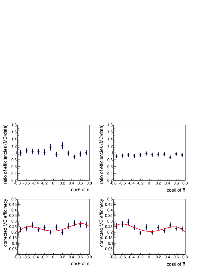
Figure 1: (Top row) Ratios of the detection efficiencies between MC simulation and data vs $\cos\theta$ for neutron and antineutron, and (bottom row) the corrected detection efficiencies to select the $\psi(3686)\to n\bar{n}$ events vs $\cos\theta$. The solid curves are the fit results with a fourth-order polynomial function. The left plots are for the neutron, and the right ones are for the antineutron.

III.4 Branching fraction and angular distribution

We perform a fit to the $\theta_{\mathrm{open}}$ distribution of data to obtain the numbers of signal candidates and background events. The histogram from signal MC simulation is used to construct the signal probability density function (PDF). Corresponding histograms from the three background components, as described in Sec. III.2, are used to construct the background PDFs. The numbers of events from each source are free parameters in the fit. Figure 2 shows the fit to the $\theta_{\mathrm{open}}$ distribution. The fit yields $N_{sig}=6056\pm 117$ $n\bar{n}$ events with $\chi^{2}/ndf=3.24$. Using a corrected efficiency $\epsilon=18.5\%$, the branching fraction of $\psi(3686)\to n\bar{n}$ is determined to be $(3.06\pm 0.06)\times 10^{-4}$ via $\mathcal{B}=N_{sig}/(N_{\psi(3686)}\epsilon)$, where $N_{\psi(3686)}$ is the total number of $\psi(3686)$ and the uncertainty is statistical only.

We fit the $\cos\theta_{n}$ and $\cos\theta_{\bar{n}}$ distributions separately with fixed fractions of each component to determine the $\alpha$ values. For these fits, an additional selection criterion $\theta_{\mathrm{open}}>3.01$ is used to further suppress the continuum background, and the fractions of each components within the region $3.01<\theta_{\mathrm{open}}<3.20$ are obtained from the $\theta_{\mathrm{open}}$ fit results. For the $\cos\theta_{n}$ and $\cos\theta_{\bar{n}}$ distributions, the background PDFs are constructed with the same method as used in the fits to $\theta_{\mathrm{open}}$, while the signal PDF is constructed by the formula $(1+\alpha\cos^{2}\theta)\epsilon(\theta)$. Here, $\epsilon(\theta)$ is the corrected polar angle-dependent efficiency parameterized in a fourth-order polynomial, as described in Sec. III.3. Figure 3 shows the fits to the $\cos\theta_{n}$ and $\cos\theta_{\bar{n}}$ distributions. An average $\alpha_{n\bar{n}}=0.68\pm 0.12$ for the angular distribution is obtained, while the separate fit results are $0.76\pm 0.12$ ($\chi^{2}/ndf=0.81$) and $0.60\pm 0.12$ ($\chi^{2}/ndf=2.01$) for the $\cos\theta_{n}$ and $\cos\theta_{\bar{n}}$ distributions, respectively. The uncertainties here are statistical only. Since the neutron and antineutron are back to back in the c.m. system and the two angular distributions are fully correlated, the average does not increase the statistics, and the uncertainty is not changed.

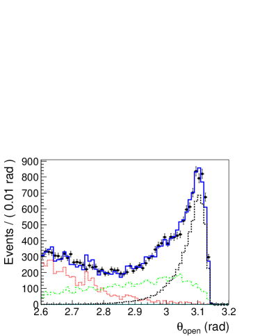
Figure 2: Fit to the $\theta_{\mathrm{open}}$ distribution. The data are shown by the dots with error bars. The fit result is shown as the solid blue curve. The signal shape is from MC simulation and is presented as the dashed black histogram. The background is described by three components: continuum background in dotted red, inclusive MC sample in dash-dotted green, and the tiny contribution from $\psi^{\prime}\to\gamma\chi_{cJ},\chi_{cJ}\to n\bar{n}$ (not included in the inclusive MC sample) in long-dashed cyan. All yields are free parameters in the fit.

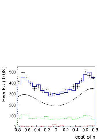
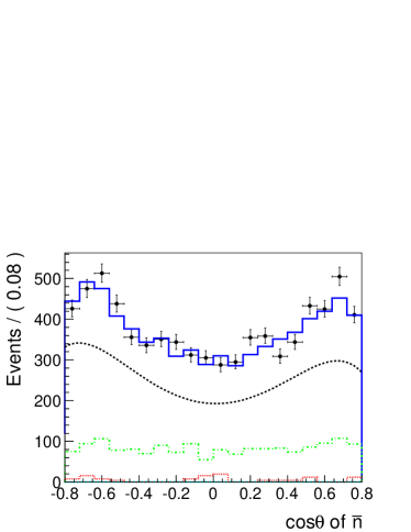
Figure 3: Individual fits to the $\cos\theta$ distributions of (left) neutron and (right) antineutron. Data are shown as dots with error bars. The fit result is shown as the solid blue curve. The signal shape is parametrized by $(1+\alpha\cos^{2}\theta)\epsilon(\theta)$, shown as the dashed black curve. The background is described by three components: continuum background in dotted red, inclusive MC sample in dash-dotted green, and a small contribution from $\psi^{\prime}\to\gamma\chi_{cJ},\chi_{cJ}\to n\bar{n}$ in long-dashed cyan.

III.5 Systematic uncertainties

III.5.1 Resolution of $\theta_{\mathrm{open}}$

To determine the difference in the $\theta_{\mathrm{open}}$ resolution between data and MC, we fit the $\theta_{\mathrm{open}}$ distribution of data with the signal PDF convolved with a Gaussian function of which the parameters are left free in the fit. The resultant mean and width of the Gaussian function are $0.005$ and $0.002$ rad, respectively. With these modified PDFs, the resultant changes are $0.3\%$ for the branching fraction and $0.0\%$ for the $\alpha$ value, which are taken as the systematic uncertainties from the resolution of $\theta_{\mathrm{open}}$. We do not consider the resolution effect for the $\cos\theta$ distributions because of their smoother shapes.

III.5.2 Backgrounds

The uncertainties associated with the background amplitudes are estimated by fitting the $\theta_{\mathrm{open}}$ distribution with fixed contributions for the continuum and inclusive MC background. The differences between the new results and the nominal ones, $0.8\%$ and $8.1\%$ for the branching fraction and the $\alpha$ value, respectively, are taken as the systematic uncertainties related with the background amplitudes.

To estimate the effect on the $\alpha$ distribution from the continuum background shape, we redo the fit to the $\cos\theta$ distributions with the shape of the continuum background obtained without the additional requirement $\theta_{\mathrm{open}}>3.01$, assuming that there is no correlation between $\theta_{\mathrm{open}}$ and $\cos\theta$. The difference of $\alpha$ to the nominal result is $4.4\%$.

All in all, we determine the uncertainty from backgrounds to be $0.8\%$ for the branching fraction and $9.2\%$, the quadratic sum of $8.1\%$ and $4.4\%$, for $\alpha$.

III.5.3 Neutral reconstruction efficiencies

The reconstruction efficiency is corrected in bins of $\cos\theta$, and the uncertainty of the correction is taken to be the statistical uncertainty, which is about 2% per $\cos\theta$ bin. To obtain its effect on our results, we allow the efficiency to fluctuate about the corrected efficiency according to the statistical uncertainty, and redo the fits with the modified efficiencies. We also use the histograms of the corrected MC efficiencies directly. The largest change of the signal yield is $0.2\%$ with the average efficiency changing by $2\%$ ($1\%$ each from $\bar{n}$ and $n$), and the largest change in $\alpha$ is $12.8\%$. We take these differences from the standard results as the systematic uncertainties of the neutral efficiency correction.

III.5.4 Remaining showers

We have checked and found that the number and energy of remaining showers are independent of the angle, as we expected. Then only the branching fraction measurement will be affected by the unperfect MC simulation. Based on the distributions of the number and energy of remaining showers from the data, we weight them in the signal MC considering their correlation. The difference is found to be $0.4\%$ by comparing the efficiencies obtained with and without weighting, and is quoted as the corresponding uncertainty.

III.5.5 Analysis method

We perform input/output checks by generating different signal MC samples with different $\alpha$ values, from zero to unity; mixing these signal MC samples with backgrounds; and scaling these samples to the number of events according to data. Compared to the input values, the output signal yield is very close to the input, and its corresponding systematic uncertainty can be neglected. For the measurement of $\alpha$, the average difference, $2\%$, is taken as the systematic uncertainty.

III.5.6 Binning

In the nominal analysis, the $\theta_{\mathrm{open}}$, $\cos\theta_{n}$, and $\cos\theta_{\bar{n}}$ distributions are divided into 60, 20 and 20 bins, respectively. To estimate the uncertainty associated with binning, we redivide the distributions of $\theta_{\mathrm{open}}$, $\cos\theta_{n}$, and $\cos\theta_{\bar{n}}$ into $[55,65]$, $[18,22]$, $[18,22]$ bins, respectively and perform $11\times 5\times 5=275$ fits of $\theta_{\mathrm{open}}$, $\cos\theta_{n}$, and $\cos\theta_{\bar{n}}$ with all possible combinations of binnings to determine the signal yields and $\alpha$ values. The differences between the average results and the nominal values, $0.1\%$ for the branching fraction and $4.5\%$ for the $\alpha$ value, are taken as the systematic uncertainties.

III.5.7 Physics model

The signal efficiency in the branching fraction measurement depends on the value of $\alpha$. Varying $\alpha$ by its standard deviation, the relative change on the detection efficiency, $1.1\%$, is taken as the systematic uncertainty due to the physics model.

III.5.8 Trigger efficiency

The neutral events used for this analysis are selected during data taking by two trigger conditions: 1) the number of clusters in the EMC is required to be greater than one, and 2) the total energy deposited in the EMC is greater than $0.5\ \mathrm{GeV}$ Berger:2010my . The efficiency of the former condition is very high Berger:2010my , and we conservatively take $2\%$ as its systematic uncertainty. Requiring the EMC total energy to be larger than $0.9\ \mathrm{GeV}$, the trigger efficiency of the second condition is $98.8\%$ Berger:2010my , with an uncertainty of $1.2\%$. Comparing the nominal results to the results with the higher total energy requirement, the difference is $0.2\%$. Combining the two gives $1.4\%$, which is taken as the systematic uncertainty of the second trigger condition. Since these two trigger conditions may be highly correlated, we take a conservative $3.4\%$ as the total systematic uncertainty of the trigger.

III.5.9 Number of $\psi(3686)$ events

The systematic uncertainty on the number of $\psi(3686)$ events is $0.7\%$ Ablikim:2012pj .

III.5.10 Summary of systematic uncertainties

The systematic uncertainties in the measurements of $\psi(3686)\to n\bar{n}$ are summarized in Table 3. Assuming these systematic uncertainties are independent of each other, the total uncertainty is obtained by adding the individual uncertainties quadratically.

Table 3: The relative systematic uncertainties for $\psi(3686)\to n\bar{n}$. Here ”$\cdots$” denotes negligible.

Item	Br ($\%$)	$\alpha$ ($\%$)
Resolution	$0.3$	$\cdots$
Background	$0.8$	$9.2$
Neutrals Efficiency	$2.2$	$12.8$
Remaining Showers	$0.4$	$\cdots$
Method	$\cdots$	$2.0$
Binning	$0.1$	$4.5$
Physics model	$1.1$	$\cdots$
Trigger	$3.4$	$\cdots$
Number of $\psi^{\prime}$	$0.7$	$\cdots$
Total	$4.4$	$16.5$

IV Measurement of $\psi(3686)\to p\bar{p}$

IV.1 Event selection

The final state of $\psi(3686)\to p\bar{p}$ consists of a proton and an antiproton, which are back to back and with a fixed momentum in the c.m. system. A candidate charged track, reconstructed in the MDC, is required to satisfy $V_{r}<1.0$ cm and $|V_{z}|<10.0$ cm, where $V_{r}$ and $V_{z}$ are the distances of closest approach of the reconstructed track to the interaction point, projected in a plane transverse to the beam and along the beam direction, respectively. Two charged track candidates with net charge zero are required. We also require the momentum of each track to satisfy $1.546<p<1.628\ \mathrm{GeV}/c$ in the c.m. system, which is within three times the resolution of the expected momentum, and the polar angle to satisfy $|\cos\theta|<0.8$. Using the information from the barrel TOF, likelihoods $\mathcal{L}_{i}$ for different particle hypotheses are calculated, and the likelihood of both the proton and antiproton must satisfy $\mathcal{L}_{p}>0.001$ and $\mathcal{L}_{p}>\mathcal{L}_{K}$, where $\mathcal{L}_{p}$ is the PID likelihood for the proton or antiproton hypothesis, and $\mathcal{L}_{K}$ is the likelihood for the kaon hypothesis. Further, we require the opening angle of the two tracks to satisfy $\theta_{\mathrm{open}}>3.1\ \mathrm{rad}$ in the $\psi(3686)$ c.m. system. There are $18,984$ candidate events satisfying the selection criteria, which are used for the further study.

IV.2 Background estimation

In the analysis, backgrounds from the continuum process $e^{+}e^{-}\to p\bar{p}$ and $\psi(3686)$ decay into non-$p\bar{p}$ final states are explored with different approaches. The former background is studied with the off-resonance data at $\sqrt{s}=3.65$ GeV. With the same selection criteria, there are $(22\pm 5)$ events that survive, and the expected background in the $\psi(3686)$ data is $(22\pm 5)\times 3.7=81\pm 18$ events, where $3.7$ is the scale factor which is the same as in the $n\bar{n}$ study. By imposing the same selection criteria on the $\psi(3686)$ inclusive MC sample, no non-$p\bar{p}$ final state events survive, and the non-$p\bar{p}$ final state background from $\psi(3686)$ decays is negligible. We also check the latter background with the two-dimensional sidebands of the proton versus antiproton momenta, which is shown in Fig. 4. There are a few events in the sideband regions, marked as A and B in Fig. 4, but MC studies indicate that the events are dominantly initial state or final state radiation events of $\psi(3686)\to p\bar{p}$. The ratios of events in each sideband region to that in signal region are consistent between data and signal MC simulation.

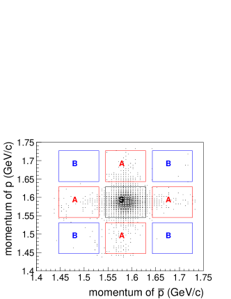
Figure 4: Scatter plots of momenta of proton vs antiproton. The left plot is data, and the right one is for inclusive MC.

IV.3 Efficiency correction

In the $\psi(3686)\to p\bar{p}$ analysis, we correct the MC efficiency as a function of $\cos\theta$ of the proton and antiproton, where the corrected factors include both for tracking and PID efficiencies. The efficiency differences between data and MC simulation, which are obtained by studying the same control sample of $\psi(3686)\to p\bar{p}$, are taken as the correction factors. To determine the efficiency for the proton, we count the number of $\psi(3686)\to p\bar{p}$ events by requiring an antiproton only, and then check if the other track is reconstructed successfully in the recoiling side and passes the PID selection criterion. The efficiency is defined as $n_{2}/(n_{1}+n_{2})$, where $n_{1}$ and $n_{2}$ are the yields of events with only one reconstructed track identified as an antiproton and with two reconstructed tracks identified as proton and antiproton, respectively. The yields $n_{1}$ and $n_{2}$ are obtained from fits to the antiproton momentum distributions. In the fit, the signal shape is described by the momentum distribution of the antiproton with the standard selection criteria for $\psi(3686)\to p\bar{p}$, and the background is described by a first-order polynomial function since it is found to be flat from a study of the inclusive MC sample. Cosmic rays and beam-related backgrounds are subtracted using $V_{z}$-sidebands, in which $|V_{z}|\leq 5\ \mathrm{cm}$ is defined as the signal region and $(-10<V_{z}<-5)$ and $(5<V_{z}<10)$ are defined as sideband regions. A similar analysis is performed for the antiproton detection efficiency. The ratio of efficiencies between MC simulation and data are displayed individually in Fig. 5 for the proton and antiproton. We obtain the corrected MC efficiency to select $\psi(3686)\to p\bar{p}$ candidates, also shown in Fig. 5. The corrected MC efficiencies are fitted with fourth-order polynomial functions with $\chi^{2}/ndf=2.56$ and $2.57$ for the proton and antiproton, respectively.

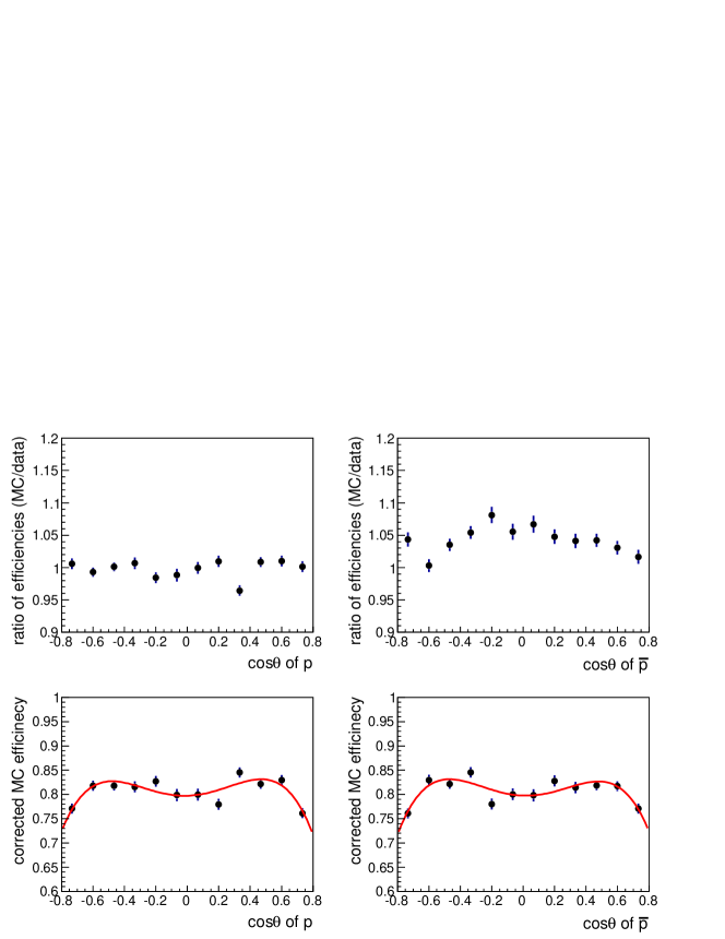
Figure 5: (Top row) Ratios of efficiencies of MC simulation over data and (bottom row) the corrected MC efficiency to select the signal events $\psi(3686)\to p\bar{p}$. The left plots are for the proton, and the right ones are for the antiproton.

IV.4 Branching fraction and angular distribution

After subtracting the continuum background, the branching fraction is determined to be $\mathcal{B}(\psi(3686)\to p\bar{p})=(3.05\pm 0.02)\times 10^{-4}$ via $\mathcal{B}=N_{sig}/(N_{\psi(3686)}\epsilon)$ with the corrected efficiency of $\epsilon=58.1\%$ determined with the angular distribution corresponding to the value of $\alpha$ obtained in this analysis. The $\cos\theta$ distributions of the proton and anti-proton for the selected candidates are shown in Fig. 6. The distributions are fitted with the functional form $N_{\text{sig}}(1+\alpha\cos^{2}\theta)\epsilon(\theta)+N_{\text{bg}}f_{\text{bg}}$, where $N_{\text{bg}}$ and $f_{\text{bg}}$, the yield and the shape of the continuum background, are fixed in the fit according to the off-resonance data at $\sqrt{s}=3.65\ \mathrm{GeV}$. The fits are performed individually to the $\cos\theta$ distributions of the proton and anti-proton and yield the same value of $\alpha=1.03\pm 0.06$ with $\chi^{2}/ndf$ $1.06$ and $0.82$, respectively.

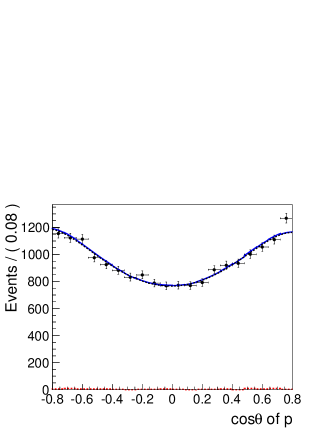
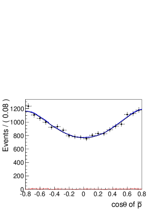
Figure 6: Fits to the $\cos\theta$ distributions of the (left) proton and (right) anti-proton. The dots with error bars are data, the solid blue lines are the fit curves, and the dashed red lines at the bottom of each plot are the backgrounds.

IV.5 Systematic uncertainties

IV.5.1 Momentum resolution

In this analysis, there are two requirements on the momentum, $\theta_{\text{open}}>3.1$ and $1.546<p<1.628\ \mathrm{GeV}/c$, which involve both its direction and magnitude.

We smear the momentum direction for the MC sample to improve the consistency of the $\theta_{\text{open}}$ distributions between data and MC simulation. The detection efficiencies for the requirement $\theta_{\mathrm{open}}>3.1$ are $98.1\%$ and $97.8\%$ without and with the direction smearing, respectively. Thus, the systematic uncertainty for the branching fraction measurement from this effect is taken as $0.3\%$.

By fitting the momentum distributions of the proton and anti-proton, the momentum resolutions are found to be $13.5$ and $11.2\ \mathrm{MeV}/c$ for data and MC simulation, respectively. The corresponding efficiencies for the requirement $1.546<p<1.628\ \mathrm{GeV}/c$ are $99.76\%$ and $99.97\%$ for the data and MC simulation, respectively, where the efficiencies are estimated by integrating the Gaussian function within the specific signal regions. Thus, the systematic uncertainty is taken to be $0.4\%$ for the two charged tracks.

The total systematic uncertainty associated with the momentum resolution for the branching fraction is $0.5\%$, and that for the $\alpha$ value measurement is found to be negligible.

IV.5.2 Background

The dominant background is from the continuum process, which is estimated with the off-resonance data sample at $\sqrt{s}=3.65\ \mathrm{GeV}$. The corresponding uncertainty of $18$ events, which is $0.1\%$ of all signal events, is taken as the uncertainty in the branching fraction measurement associated with the background. The uncertainty on the $\alpha$ value associated with background is studied by leaving the background yield free in the fit and found to be negligible.

IV.5.3 Tracking and PID efficiencies

In the nominal analysis, the tracking and PID efficiencies for the proton and anti-proton are corrected to improve the accuracy of the measurement. Thus, only the uncertainties associated with the statistics of correction factors and the method to exact correction factors are considered.

We repeat the analysis $1000$ times by randomly fluctuating the correction factors for the proton and anti-proton detection efficiency with Gaussian functions independently in the different $\cos\theta$ bins, where the width of the Gaussian function is the statistical uncertainty of the correction factors. The standard deviations of the results are $<0.1\%$ for the branching fraction and $0.2\%$ for $\alpha$, which are taken as the systematic uncertainties associated with the statistical uncertainties.

In the nominal analysis, the corrected efficiency is parametrized with a fourth-order polynomial function. Alternative parametrizations with a polynomial function symmetric in $\cos\theta$ and directly using the histogram for the corrected efficiency are performed. The maximum changes of the branching fraction and $\alpha$ value, $3.3\%$ and $2.1\%$, respectively, are taken as the systematic uncertainties.

To be conservative, the linear sums of the two uncertainties, $3.3\%$ and $2.3\%$, are taken as the systematic uncertainties for the branching fraction and $\alpha$ measurements associated with the tracking and PID efficiency, respectively.

IV.5.4 Method

From input/output checks, the average relative differences between measured and true values are $1.1\%$ for the branching fraction and $2.0\%$ for $\alpha$, which are taken as the systematic uncertainties.

IV.5.5 Binning

In the nominal analysis, the $\cos\theta$ range of the proton and anti-proton of $(-0.8,0.8)$ is divided into $20$ bins to determine the corrected tracking and PID efficiency. Alternative analyses with $10$ or $40$ bins are also performed, and the largest differences with respect to the nominal results are taken as the systematic uncertainties associated with binning. The effect is negligible for the branching fraction measurement and $1.0\%$ for the $\alpha$ measurement.

IV.5.6 Physics model

In the branching fraction measurement, the detection efficiency depends on the value of $\alpha$. Alternative detection efficiencies varying $\alpha$ from $0.96$ to $1.10$, corresponding to one standard deviation, are used. The largest change of the efficiency with respect to the nominal value, $1.8\%$, is taken as the systematic uncertainty.

IV.5.7 Trigger efficiency

Events with two high momentum charged tracks in the barrel region of the MDC have trigger efficiencies of $100.0\%$ and $99.94\%$ for Bhabha and dimuon events Berger:2010my , respectively, and the systematic uncertainty from the trigger is negligible.

IV.5.8 Number of $\psi(3686)$ events

The systematic uncertainty on the number of $\psi(3686)$ events is $0.7\%$ Ablikim:2012pj .

IV.5.9 Summary of systematic uncertainties

The systematic uncertainties of $\psi(3686)\to p\bar{p}$ from the different sources are summarized in Table 4. Assuming the systematic uncertainties are independent, the total uncertainty is the sum on the individual values added in quadrature.

Table 4: Relative systematic uncertainties for the measurement of $\psi(3686)\to p\bar{p}$ in $\%$, where “$\cdots$” in the table means negligible.

	Br ($\%$)	$\alpha$ ($\%$)
Resolution	$0.5$	$\cdots$
Background	$0.1$	$\cdots$
Tracking and PID	$3.3$	$2.3$
Method	$1.1$	$2.0$
Binning	$\cdots$	$1.0$
Physics model	$1.8$	$\cdots$
Trigger	$\cdots$	$\cdots$
Number of $\psi(3686)$	$0.7$	$\cdots$
Total	4.0	3.2

V Summary and Discussion

In this paper, we measure the branching fractions of $\psi(3686)\to n\bar{n}$ and $p\bar{p}$, and the $\alpha$ values of the polar angle distribution, which are described by $1+\alpha\cos^{2}\theta$. The final results are $\mathcal{B}(\psi(3686)\to n\bar{n})=(3.06\pm 0.06\pm 0.14)\times 10^{-4}$ and $\alpha_{n\bar{n}}=0.68\pm 0.12\pm 0.11$, and $\mathcal{B}(\psi(3686)\to p\bar{p})=(3.05\pm 0.02\pm 0.12)\times 10^{-4}$ and $\alpha_{p\bar{p}}=1.03\pm 0.06\pm 0.03$, where the former process is measured for the first time and the latter one has improved precision compared to previous measurements, as summarized in Table 1. The measured $\alpha_{p\bar{p}}$ is close to $1.0$, which is larger than previous measurements, but both $\mathcal{B}(\psi(3686)\to p\bar{p})$ and $\alpha_{p\bar{p}}$ are consistent with previous results within the uncertainties.

To check for an odd $\cos\theta$ contribution from the $2\gamma$ exchange process Pacetti:2015iqa , we fit the angular distributions as before but with the function $1+\beta\cos\theta+\alpha\cos^{2}\theta$. The results are $\beta_{n\bar{n}}=0.04\pm 0.05$ and $\beta_{p\bar{p}}=0.01\pm 0.02$. The possible contributions from odd $\cos\theta$ terms in this analysis are consistent with zero.

With the assumption the decay process is via a single photon exchange, the $\alpha$ value must satisfy $|\alpha|\leq 1$ Faldt:2017kgy . Then, the formula $1+\sin\phi\cos^{2}\theta$ is applied to fit to the $p\bar{p}$ data again, and we obtain the result $\phi_{p\bar{p}}=1.57\pm 0.28\pm 0.25$, where the statistical uncertainty is obtained from fit directly and the systematical uncertainty is propagated from the $3.2\%$ of the $\alpha_{p\bar{p}}$ value.

To compare with the 12% rule, we use our measured branching fractions to obtain

$$\frac{\mathcal{B}(\psi(3686)\to p\bar{p})}{\mathcal{B}(J/\psi\to p\bar{p})}=(14.4\pm 0.6)\%$$

and

$$\frac{\mathcal{B}(\psi(3686)\to n\bar{n})}{\mathcal{B}(J/\psi\to n\bar{n})}=(14.8\pm 1.2)\%,$$

where $\mathcal{B}(J/\psi\to p\bar{p})=(2.120\pm 0.029)\times 10^{-3}$ and $\mathcal{B}(J/\psi\to n\bar{n})=(2.09\pm 0.16)\times 10^{-3}$ are the world average results pdg2015 . Both ratios are consistent with the 12% rule.

In the decay of $J/\psi\to n\bar{n}$ and $p\bar{p}$ pdg2015 , both the branching fractions and $\alpha$ values are very close between the two decay modes, which is expected if the strong interaction is dominant in $J/\psi\to N\bar{N}$ decay and the relative phase of between the strong and electromagnetic amplitudes is close to $90^{\circ}$  Ablikim:2012eu . In contrast, in $\psi(3686)$ decays, the branching fractions are quite close between the two decay modes, but the $\alpha$ values are not, which may imply a more complex mechanism in the decay of $\psi(3686)\to N\bar{N}$. It makes a similar and straightforward extraction of the phase angle impossible in the decay of $\psi(3686)\to N\bar{N}$, and further studies are deserved.

- (1) D. M. Asner et al., Int. J. Mod. Phys. A 24, S1 (2009)
- (2) G. J. Feldman and M. L. Perl, Phys. Rep. 33, 285 (1977).
- (3) M. Ablikim et al. (BESIII Collaboration), Chin. Phys. C 37, 063001 (2013)
- (4) K. Zhu, X. H. Mo, and C. Z. Yuan, Int. J. Mod. Phys. A 30, 1550148 (2015)
- (5) M. Suzuki, Phys. Rev. D 60, 051501 (1999)
- (6) G. Lopez Castro, J. L. Lucio M. and J. Pestieau, AIP Conf. Proc. 342, 441 (1995)
- (7) L. Köpke and N. Wermes, Phys. Rep. 174, 67 (1989).
- (8) J. Jousset et al. (DM2 Collaboration), Phys. Rev. D 41, 1389 (1990).
- (9) D. Coffman et al. (MARK-III Collaboration), Phys. Rev. D 38, 2695 (1988); 40, 3788(E) (1989).
- (10) H. E. Haber and J. Perrier, Phys. Rev. D 32, 2961 (1985).
- (11) J. Adler et al. (MARK-III Collaboration), in 1987 Europhys. Conference on High Energy Physics, Uppsala, Sweden, 1987 (unpublished).
- (12) R. Baldini et al., Phys. Lett. B 444, 111 (1998).
- (13) M. Ablikim et al. (BESIII Collaboration), Phys. Rev. D 86, 032014 (2012)
- (14) J. M. Gerard and J. Weyers, Phys. Lett. B 462, 324 (1999)
- (15) M. Suzuki, Phys. Rev. D 63, 054021 (2001).
- (16) C. Z. Yuan, P. Wang and X. H. Mo, Phys. Lett. B 567, 73 (2003)
- (17) P. Wang, C. Z. Yuan, X. H. Mo and D. H. Zhang, Phys. Lett. B 593, 89 (2004)
- (18) P. Wang, C. Z. Yuan and X. H. Mo, Phys. Rev. D 69, 057502 (2004)
- (19) P. Kessler, Nucl. Phys. B15, 253 (1970).
- (20) S. J. Brodsky and G. P. Lepage, Phys. Rev. D 24, 2848 (1981).
- (21) I. Peruzzi et al., Phys. Rev. D 17, 2901 (1978).
- (22) M. Claudson, S. L. Glashow and M. B. Wise, Phys. Rev. D 25, 1345 (1982).
- (23) C. Carimalo, Int. J. Mod. Phys. A 02, 249 (1987).
- (24) F. Murgia and M. Melis, Phys. Rev. D 51, 3487 (1995)
- (25) J. Bolz and P. Kroll, Eur. Phys. J. C 2, 545 (1998)
- (26) C. Patrignani et al. (Particle Data Group), Chin. Phys. C, 40, 100001 (2016) and 2017 update.
- (27) M. Ambrogiani et al. (Fermilab E835 Collaboration), Phys. Lett. B 610, 177 (2005)
- (28) M. Ablikim et al. (BES Collaboration), Phys. Lett. B 648, 149 (2007)
- (29) T. K. Pedlar et al. (CLEO Collaboration), Phys. Rev. D 72, 051108 (2005)
- (30) J. P. Lees et al. (BaBar Collaboration), Phys. Rev. D 88, 072009 (2013)
- (31) S. Dobbs, A. Tomaradze, T. Xiao, K. K. Seth and G. Bonvicini, Phys. Lett. B 739, 90 (2014)
- (32) M. Ablikim et al. (BES Collaboration), Phys. Lett. B 632, 181 (2006)
- (33) M. Ablikim et al. (BESII Collaboration), Chin. Phys. C 36, 1031 (2012).
- (34) M. Ablikim et al. (BESIII Collaboration), Phys. Lett. B 770, 217 (2017)
- (35) M. Ablikim et al. (BESIII Collaboration), Phys. Rev. D 93, 072003 (2016)
- (36) T. Appelquist and H. D. Politzer, Phys. Rev. Lett., , 43 (1975).
- (37) A. De Rùjula and S. L. Glashow, Phys. Rev. Lett., , 46 (1975).
- (38) M. E. B. Franklin et al., Phys. Rev. Lett. 51, 963 (1983).
- (39) Y. F. Gu and X. H. Li, Phys. Rev. D 63, 114019 (2001)
- (40) N. Brambilla et al., Eur. Phys. J. C 71, 1534 (2011)
- (41) Q. Wang, G. Li and Q. Zhao, Phys. Rev. D 85, 074015 (2012)
- (42) M. Ablikim et al. (BESIII Collaboration), Nucl. Instrum. Methods Phys. Rev. Sect. A 614, 345 (2010).
- (43) S. Jadach, B. F. L. Ward and Z. Was, Comput. Phys. Commun. 130, 260 (2000); Phys. Rev. D 63, 113009 (2001).
- (44) D. J. Lange, Nucl. Instrum. Methods Phys. Rev. Sect. A 462, 152 (2001);
- (45) R. G. Ping et al., Chin. Phys. C 32, 599 (2008).
- (46) J. C. Chen, G. S. Huang, X. R. Qi, D. H. Zhang and Y. S. Zhu, Phys. Rev. D 62, 034003 (2000).
- (47) S. Agostinelli et al. (geant4 Collaboration), Nucl. Instrum. Methods Phys. Rev. Sect. A 506, 250 (2003).
- (48) Z. Y. Deng et al., High Energy Physics and Nuclear Physics 30, 371 (2006).
- (49) http://root.cern.ch
- (50) A. Hoecker, P. Speckmayer, J. Stelzer, J. Therhaag, E. von Toerne, and H. Voss, “TMVA: Toolkit for Multivariate Data Analysis,” PoS ACAT 040 (2007) [arxiv:0703039 [physics]].
- (51) J. R. Quinlan, in Proceedings of the Thirteenth National Conference on Artificial Intelligence, Portland, Oregon, 1996.
- (52) N. Berger, K. Zhu, Z. -A. Liu, D. -P. Jin, H. Xu, W. -X. Gong, K. Wang and G. -F. Cao, Chin. Phys. C 34, 1779 (2010)
- (53) S. Pacetti, R. Baldini Ferroli and E. Tomasi-Gustafsson, Phys. Rep. 550-551, 1 (2015).
- (54) G. Fäldt and A. Kupsc, Phys. Lett. B 772, 16 (2017)