Excitation mechanism of O i lines in Herbig Ae/Be stars

Abstract

We have investigated the role of a few prominent excitation mechanisms viz. collisional excitation, recombination, continuum fluorescence and Lyman beta fluorescence on the O i line spectra in Herbig Ae/Be stars. The aim is to understand which of them is the central mechanism that explains the observed O i line strengths. The study is based on an analysis of the observed optical spectra of 62 Herbig Ae/Be stars and near-infrared spectra of 17 Herbig Ae/Be stars. The strong correlation observed between the line fluxes of O i $\lambda$8446 and O i $\lambda$11287, as well as a high positive correlation between the line strengths of O i $\lambda$8446 and H$\alpha$ suggest that Lyman beta fluorescence is the dominant excitation mechanism for the formation of O i emission lines in Herbig Ae/Be stars. Further, from an analysis of the emission line fluxes of O i $\lambda\lambda$7774, 8446, and comparing the line ratios with those predicted by theoretical models, we assessed the contribution of collisional excitation in the formation of O i emission lines.

1 Introduction

Herbig Ae/Be (HAeBe) stars are intermediate mass ($2~{}M_{\odot}\leq M\leq 8~{}M_{\odot}$) pre-main sequence stars with accretion disks, the innermost regions of which also act as a reservoir for the production of major emission lines seen in the optical and infrared spectra (Herbig, 1960; Hillenbrand et al., 1992; Waters & Waelkens, 1998). HAeBe stars were first discussed as a distinct group of objects by Herbig (1960), who noted that they were stars of spectral type A or B with emission lines, located in an obscured region and often accompanied by a surrounding nebulosity. The present working definition of HAeBe stars includes, (a) pre-main sequence stars of A$-$F spectral type, displaying emission lines in their spectra and (b) show a significant IR excess due to hot or cool circumstellar dust shell or a combination of both (The et al., 1994; Waters & Waelkens, 1998; Vieira et al., 2003). There have been extensive spectroscopic studies of HAeBe stars in the literature (e.g. Hamann & Persson, 1992; Hernandez et al., 2004; Manoj et al., 2006); particularly important are the recent studies by the X-Shooter team (Mendigutía et al., 2011, 2012; Fairlamb et al., 2015, 2017). Most of these studies have been devoted to H$\alpha$ line analysis, the most prominent emission feature seen in the spectra of HAeBe stars (Finkenzeller & Mundt, 1984; Hamann & Persson, 1992). In the present study, we focus on the O i emission lines in the optical and near-infrared (1$-$2.5 micron) spectra in HAeBe stars.

O i $\lambda$8446 is the most prominent O i emission line seen in the optical spectrum of HAeBe stars. This emission line results from the 3$s^{3}S^{0}$ $-$3p${}^{3}P$ transition and is seen as a triplet at high resolution, with wavelength values of 8446.25, 8446.36 and 8446.76 Å. It is present in the spectra of a wide variety of astrophysical sources such as planetary nebulae, novae and Seyfert galaxies. A number of studies have addressed the question of excitation mechanisms of O i emission lines in various astrophysical objects. Prominent mechanisms discussed for the formation of O i lines are collisional excitation, recombination, continuum fluorescence and Lyman beta (Ly$\beta$) fluorescence. For example, Grandi (1975b) showed that starlight continuum fluorescence is the favored excitation mechanism for the O i line in the Orion nebula whereas in Seyfert 1 galaxies it is excited by Lyman $\beta$ fluorescence (Grandi, 1980). In novae, Strittmatter et al. (1977) identify Lyman $\beta$ fluorescence as the dominant excitation mechanism; a conclusion that has been supported by studies of several other novae (e.g Ashok et al., 2006; Banerjee & Ashok, 2012, and references therein). Ly$\beta$ fluorescence is identified as the dominant contributor to the emission strength of O i $\lambda$8446 line in classical Be (hereafter CBe) stars, whether it is isolated (Slettebak, 1951; Mathew et al., 2012b) or part of an X-ray binary system (Mathew et al., 2012a). Bhatia & Kastner (1995) and Kastner & Bhatia (1995) provided a theoretical framework of O i excitation and derived the expected line ratios of the prominent O i lines, when collisional excitation and Ly$\beta$ fluorescence (referred as photoexcitation by accidental resonance (PAR process) in Bhatia & Kastner, 1995) are the dominant excitation mechanisms. From a comparative analysis of the theoretical estimates with the observed emission strengths of O i $\lambda\lambda$ 7774, 8446, 11287 and 13165, Mathew et al. (2012b) demonstrated that Ly$\beta$ fluorescence is the dominant excitation mechanism for the production of O i $\lambda\lambda$ 8446, 11287 lines in CBe stars. CBe stars share similar spectral characteristics with HAeBe stars, such as emission lines of H$\alpha$, O i, Fe ii and Ca ii triplet. It is worth exploring whether both CBe and HAeBe stars share similar excitation mechanism for the formation of O i lines. There could be considerable difference between the O i line forming regions in both the stellar systems. CBe stars are found to have a circumstellar gaseous decretion disk wherein O i $\lambda$8446 line is formed at a mean radial distance of $\sim$8 $R_{\star}$, considering Keplerian motion (Mathew et al., 2012b). However, the location of the origin of O i $\lambda$8446 line in HAeBe is far from clear. Most of the accretion related emission lines in HAeBe stars (e.g. H$\alpha$, Pa$\beta$, Br$\gamma$) are thought to be formed in the magnetospheric accretion columns (Muzerolle et al., 2004). This work is an attempt to bring more clarity to our understanding of the formation mechanisms of O i emission lines in HAeBe stars.

The paper is organized as follows. In Section 2 we present the optical and near-infrared (near-IR) spectroscopic observations carried out over a period of 3 years and describe the data reduction techniques employed. We describe the methods and the python routines used for the spectral analysis and to estimate line flux in Section 3. The dominant excitation mechanism for the formation of O i lines in HAeBe stars is evaluated in Section 4. The main results of the paper are summarized in Section 5.

2 Observations and data reduction

The optical spectroscopic observations were carried out using the Himalayan Faint Object Spectrograph Camera (HFOSC) mounted on the 2-m Himalayan Chandra Telescope (HCT). The spectroscopic observations were obtained with Grism 8 in combination with 167$l$ slit (1.92$\arcsec$ wide and 11$\arcmin$ long), providing an effective resolving power of $\sim$ 1050. The spectral coverage is from 5500 to 9000 Å, which included the spectral lines relevant to this study, viz., H$\alpha$, O i $\lambda$7774 and O i $\lambda$8446. After each on-source exposure, FeNe lamp spectra were obtained for wavelength calibration. We have followed the regular procedure of reducing the spectra after bias subtraction and flat-field correction using the standard tasks in Image Reduction and Analysis Facility (IRAF).

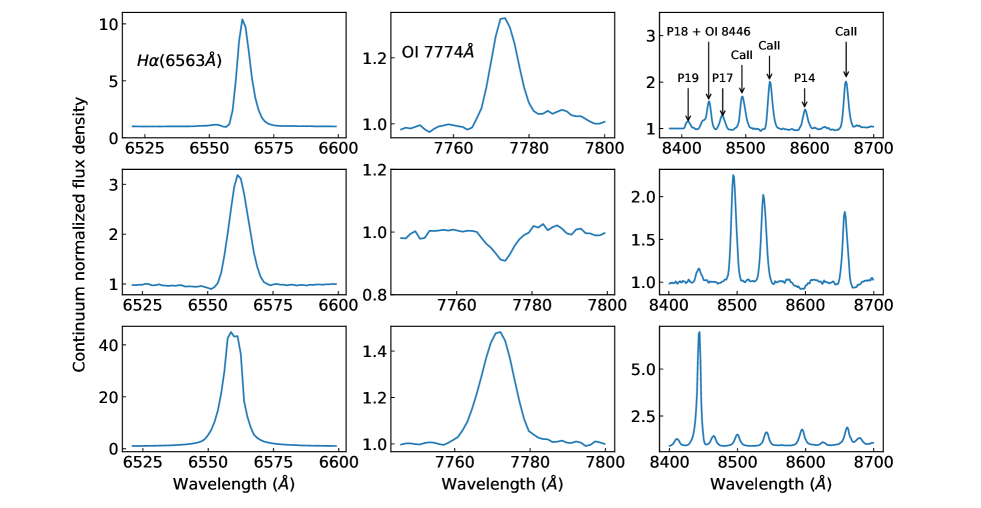
Figure 1: Observed spectra of V594 Cas, LkH$\alpha$ 233 and MWC 297 (top to bottom). The line profiles of H$\alpha$, O i $\lambda$7774 and O i $\lambda$8446 are shown in each case (left to right). Ca ii triplet (8498, 8542, 8662 Å) lines are seen in most spectra and appears to be blended with Paschen lines when they are in emission.

Near-IR spectra were obtained using the TIFR Near Infrared Spectrometer and Imager (TIRSPEC), mounted on the HCT. The spectra were obtained in $Y$ and $J$ passbands, at a resolving power of 1200. The observations were performed in the dithered mode. Argon lamp spectra taken after each on-source exposure is used for wavelength calibration. An appropriate telluric standard (of early A spectral type) is observed at nearby airmass to the target object. The spectra of the target and the standard are reduced in a standard manner with the tasks in IRAF. For telluric correction, we removed the hydrogen lines from the telluric standard spectrum, which is then used to divide the object spectrum. The resultant object spectrum is multiplied with the blackbody corresponding to the spectral type of the telluric standard in order to preserve the continuum of the target spectrum. The log of optical and infrared spectroscopic observations is given in Table 1.

The sample of HAeBe stars observed were drawn from a larger list of 142 HAeBe stars that we compiled from literature (The et al., 1994; Manoj et al., 2006; Fairlamb et al., 2015). Given the location of the observatory and the limiting magnitude of the spectrograph-telescope combination, we were able to obtain the optical spectra of 56 HAeBe stars and near-IR spectra of 19 HAeBe stars. The observations were carried out over a period of 3 years, from 2014 to 2017. To increase the sample size of the present study we have included the optical spectra of HAeBe stars from Manoj et al. (2006), which were observed with similar observation setup. Thus we have optical spectra for a total of 62 HAeBe stars and near-IR spectra for 19 HAeBe stars. As a representative sample, we show H$\alpha$, O i $\lambda$ $\lambda$7774, 8446 line profiles of V594 Cas, LkH$\alpha$ 233 and MWC 297 in Figure 1.

The $B$, $V$, $R_{C}$ magnitudes, total extinction ($A_{V}$), spectral type and effective temperature ($T_{\mathrm{eff}}$) of 62 HAeBe stars are listed in Table 2. The spectral type is converted to $T_{\mathrm{eff}}$ using the tabulated information in Pecaut & Mamajek (2013). We compiled the photometric data from various sources in literature, whose references are given in Table 2. For some of the sources $R$ magnitudes are in Johnson system, which are converted to the Cousins system following Bessell (1983). The color excess, $E(B-V)$, is calculated from the observed $(B-V)$ colors and the intrinsic colors corresponding to each spectral type, from the table listed in Pecaut & Mamajek (2013). Further, we calculated $A_{V}$ from $E(B-V)$ considering a total-to-selective extinction value, $R_{V}$ = 5. It has been demonstrated from various studies (c.f. Hernandez et al., 2004) that $R_{V}$ = 5 is the preferred value in the analysis of HAeBe stars, suggesting grain growth in the disk of HAeBe stars (e.g. Gorti & Bhatt, 1993; Manoj et al., 2006)).

3 Analysis

3.1 Classification based on O i line profiles

From the observed spectra, we find that O i lines, both in optical and infrared, are seen in emission as well as in absorption. We adopted the classification scheme proposed by Felenbok et al. (1988), wherein Group I stars have both O i $\lambda$8446 and O i $\lambda$7774 in emission; Group II sources are those with both lines in absorption; Group III is the case when O i $\lambda$8446 is in emission and O i $\lambda$7774 in absorption. We found 23 stars belonging to Group I, 16 in Group II and 23 in Group III classes. Similar classification scheme is applied to the infrared spectra. Although O i emission is evident among Group I stars, after subtracting the photospheric component, a net emission is seen in some of the Group II and Group III stars. For the current sample, we found net emission in O i $\lambda\lambda$7774, 8446 for 31 and 54 stars, respectively whereas 17 sources show net emission in O i $\lambda\lambda$11287 and 13165.

Table 1: Log of spectroscopic observations

Object	Date of	Optical	Date of	$Y$ band	$J$ band
	Optical Observations	Exp.time (s)	IR Observations	Exp.time (s)	Exp.time (s)
51 Oph	2014 May. 19	60	–	–	–
AB Aur	2017 Jan. 21	40	2013 Dec. 11	600	600
AS 442	2016 Aug. 10	300	–	–	–
AS 443	2016 Aug. 10	420	–	–	–
AS 505	2016 Aug. 10	300	2016 Nov. 21	600	600
BD+30 549	2016 Nov. 22	400	–	–	–
BD+40 4124	2014 Jun. 19	300	–	–	–
BD+65 1637	2016 Aug. 10	300	–	–	–
CQ Tau	2016 Nov. 23	300	2016 Nov. 21	600	600
HBC 334	2017 Jan. 03	1800	–	–	–
HBC 551	2014 Feb. 25	1200	–	–	–
HD 141569	2014 Jun. 19	300	–	–	–
HD 142666	2014 Feb. 24	300	–	–	–
	2014 May. 19	300	–	–	–
HD 144432	2014 May. 19	300	–	–	–
HD 145718	2016 May. 15	300	–	–	–
HD 150193	2014 May. 19	600	–	–	–
	2014 Jun. 19	300	–	–	–
HD 163296	2016 May. 15	30	2016 May. 15	120	120
HD 169142	2014 May. 19	300	–	–	–
HD 190073	2014 Oct. 02	60	–	–	–
HD 200775	2017 Jan. 22	30	2016 Nov. 20	120	120
	–	–	2017 Jan. 22	320	320
HD 216629	2016 Aug. 10	30	–	–	–
HD 245185	2017 Jan. 03	600	–	–	–
HD 250550	2017 Jan. 21	600	2017 Jan. 22	600	600
HD 259431	2015 Dec. 16	60	2016 Nov. 21	600	480
HD 31648	2016 Nov. 20	60	2016 Nov. 20	180	240
HD 35187	2017 Jan. 21	60	–	–	–
HD 35929	2017 Jan. 21	120	2016 Nov. 21	480	480
HD 36112	2014 Feb. 24	180	2014 Feb. 24	120	120
	2015 Jan. 27	90	2016 Nov. 21	360	360
HD 37490	2017 Jan. 21	20	2017 Jan. 21	320	400
HD 37806	2016 Nov. 22	30	–	–	–
HD 52721	2016 Nov. 22	30	2016 Nov. 21	180	180
HD 53367	2016 Nov. 23	90	2016 Nov. 21	180	180
HK Ori	2017 Jan. 03	600	–	–	–
LkHa 167	2016 Sep. 25	1200	–	–	–
LkHa 198	2015 Dec. 16	1200	–	–	–
LkHa 224	2016 May. 16	900	–	–	–
LkHa 233	2014 Oct. 02	1800	–	–	–
LkHa 234	2016 Aug. 10	600	–	–	–
LkHa 257	2016 Aug. 10	900	–	–	–
MWC 1080	2014 Aug. 17	180	2014 Aug. 17	200	200
	2014 Nov. 02	180	–	–	–
MWC 297	2014 May. 19	360	2014 Jun. 19	120	80
	2014 Jun. 19	600	2014 Aug. 17	200	120
PDS 174	2017 Jan. 03	900	–	–	–
PX Vul	2014 Oct. 01	600	–	–	–
SV Cep	2016 Aug. 10	300	–	–	–
UX Ori	2017 Jan. 03	60	–	–	–
UY Ori	2017 Jan. 03	900	–	–	–
V1012 Ori	2017 Jan. 03	900	–	–	–
V1366 Ori	2017 Jan. 03	600	–	–	–
V376 Cas	2014 Oct. 02	1800	–	–	–
V594 Cas	2014 Oct. 01	120	2016 Nov. 20	300	400
	2014 Nov. 03	180	–	–	–
V699 Mon	2016 Nov. 23	600	–	–	–
VV Ser	2016 May. 15	1200	–	–	–
VY Mon	2017 Jan. 22	900	2017 Jan. 22	500	600
WW Vul	2016 Aug. 10	600	–	–	–
	2016 May. 15	600	–	–	–
XY Per	2016 Nov. 22	300	2017 Jan. 22	400	600
Z CMa	2014 Feb. 24	180	2014 Feb. 24	120	40

3.2 Flux measurement of O i and H$\alpha$ emission lines

In this section we describe the method we used to measure the line fluxes of H$\alpha$, O i $\lambda\lambda$7774, 8446, 11287 and 13165 lines from the wavelength calibrated optical and near-IR spectra. The procedure can be summarized as, (i) estimating the equivalent width of the lines of interest from a Gaussian profile fit using LMFIT routine in Python, (ii) removing the contribution of Paschen P18 line from O i $\lambda$8446, (iii) accounting for photospheric absorption using synthetic spectra, (iv) estimation of continuum flux at the wavelength region corresponding to H$\alpha$ and O i lines, and (v) the calculation of extinction corrected line flux from the equivalent width and the continuum flux.

3.2.1 Estimation of line equivalent width

We estimated the equivalent width (EW) of O i $\lambda\lambda$7774, 8446, 11287, 13165 and H$\alpha$ lines using the LMFIT module on the continuum subtracted, continuum normalized spectra. LMFIT, which is based on an Marquardt Levenberg nonlinear least squares minimization algorithm, was used to fit gaussians to the profiles.

3.2.2 Removal of Paschen line (P18) contribution from O i $\lambda$8446

For the spectral resolution of our observations, the line profiles of O i $\lambda$8446 and Paschen 18 (P18; 8437 Å) are blended (see Figure 1). We proposed a method in Mathew et al. (2012b) to deblend the P18 contribution from the net EW in the study of CBe stars, which will be employed here as well. The Paschen line strengths show a monotonic increase with wavelength and then display a trend of flattening out around P17 and beyond (Briot, 1981). Hence it is reasonable to obtain the EW of P18 by linearly interpolating between the measured EW of P17 (8467 Å) and P19 (8413 Å) (see Mathew et al., 2012b). This value is subtracted from the combined EW of O i $\lambda$8446 and P18 to obtain the intrinsic EW of O i $\lambda$8446.

3.2.3 Accounting for Photospheric absorption

The equivalent widths calculated from emission lines needs to be corrected for the photospheric absorption. The strength of the absorption component is estimated from the synthetic spectrum corresponding to the spectral type of the central star from Munari et al. (2005), which are calculated from the SYNTHE code (Kurucz, 1993), using NOVER models as the input stellar atmospheres (Castelli et al., 1997). The EW of underlying absorption component for H$\alpha$, O i $\lambda$7774 and O i $\lambda$8446 is estimated using the synthetic spectra corresponding to the spectral type of the star. Since the synthetic spectra of Munari et al. (2005) do not cover the infrared spectral region, we used NextGen (AGSS2009) theoretical spectra (Hauschildt et al., 1999) for the analysis of O i $\lambda\lambda$11287, 13165 line profiles. The equivalent width of the photospheric absorption is subtracted from the EW of the observed emission line to obtain the net equivalent width.

3.2.4 Estimation of line fluxes

The equivalent width of O i emission lines, corrected for photospheric absorption, needs to be multiplied with the underlying stellar continuum flux density to obtain the line flux. We are taking the extinction corrected $R$-band flux density as a proxy for the continuum flux density underlying H$\alpha$ line. The method of calculating the continuum flux density at O i emission lines from H$\alpha$ line is described below. The continuum flux density at H$\alpha$ is given as,

$$F_{\nu,cont}(H\alpha)=F_{\nu,0}\times 10^{(\frac{-R_{0}}{2.5})}$$

where $F_{\nu,0}=3.08\times 10^{-23}~{}W\ m^{-2}\ Hz^{-1}$ and R₀ is the extinction corrected $R_{C}$ magnitude. The extinction in $R$-band, $A_{R}$, is estimated from A_V using the extinction curve of McClure (2009).

Table 2: List of compiled stellar parameters for analysis of optical lines

Source	Sp. type	Ref. Sp. type	$T_{eff}$ (K)	$V$	$B-V$	$R_{C}$	Ref. Photometry	$A_{V}$
51 Oph	B9.5 IIIe	1	10400	4.78	0.03	4.75	1	0.4
AB Aur	A1	1	9200	7.05	0.12	6.92	1	0.39
AS 442	B8Ve	14	12500	10.9	0.66	10.18	3	3.85
AS 443	B2	1	20600	11.35	0.66	10.78	1	4.35
AS 505	B5Vep	15	15700	10.85	0.43	10.66	4	2.93
BD+30 549	B8p	16	12500	10.56	0.35	10.42	4	2.3
BD+40 4124	B3	1	17000	10.69	0.78	9.92	1	4.79
BD+46 3471	A0	1	9700	10.13	0.4	9.8	1	2
BD+65 1637	B4	1	16700	10.18	0.39	9.79	1	2.78
BO Cep	F4	1	6640	11.6	0.56	11.21	1	0.74
CQ Tau	F3	1	6720	10.26	0.79	9.72	1	2.01
HBC 334	B3	1	17000	14.52	0.57	13.95	1	3.74
HBC 551	B8	1	12500	11.81	0.26	11.54	1	1.85
HD 141569	A0Ve	1	9700	7.1	0.1	7.03	1	0.5
HD 142666	A8Ve	1	7500	8.67	0.5	8.34	1	1.25
HD 144432	A9IVe	1	7440	8.17	0.36	7.92	1	0.53
HD 145718	A5Ve	8	8080	9.1	0.52	8.79	2	1.8
HD 150193	A2IVe	1	8840	8.64	0.49	8.28	1	2.08
HD 163296	A1Vep	1	9200	6.88	0.09	6.82	1	0.24
HD 169142	A5Ve	1	8080	8.15	0.28	7.95	1	0.6
HD 179218	A0IVe	1	9700	7.39	0.08	7.33	1	0.4
HD 190073	A2IVe	1	8840	7.73	0.13	7.7	1	0.28
HD 200775	B3	1	17000	7.37	0.41	7.01	1	2.94
HD 216629	B3IVe+A3	17	17000	9.32	0.45	9.11	4	3.14
HD 245185	A1	1	9200	9.94	0.1	9.88	1	0.29
HD 250550	B9	1	10700	9.54	0.07	9.41	1	0.7
HD 259431	B6	1	14500	8.73	0.27	8.36	1	2.05
HD 31648	A3Ve	1	8550	7.7	0.2	7.59	1	0.55
HD 35187	A2e+A7	1	8840	8.17	0.22	76.4	1	0.73
HD 35929	F2III	1	6810	8.13	0.42	7.87	1	0.23
HD 36112	A5IVe	1	8080	8.34	0.26	8.16	1	0.5
HD 37490	B2	5	20600	4.57	-0.11	4.59	5	0.5
HD 37806	A2Vpe	1	8840	7.95	0.04	7.89	1	-0.17
HD 38120	B9	1	10700	9.01	0.06	8.93	1	0.65
HD 52721	B1	5	26000	6.62	0.06	6.53	5	1.69
HD 53367	B0IV/Ve	9	31500	6.95	0.42	6.67	2	3.64
HK Ori	A4+G1V	1	8270	11.71	0.56	11.2	1	2.1
IP Per	A6	1	8000	10.47	0.33	10.24	1	0.8
LkHa 167	A2	6	8840	15.06	1.42	14.32	4	6.73
LkHa 198	B9	1	10700	14.18	0.95	13.31	1	5.1
LkHa 224	F9	1	6040	14.07	1.44	12.98	1	4.44
LkHa 233	A4	1	8270	13.56	0.84	12.91	1	3.5
LkHa 234	B7	1	14000	12.21	0.9	11.49	1	5.14
LkHa 257	B5	7	15700	13	0.3	12.72	4	2.28
MWC 1080	B0eq	1	31500	11.52	1.34	10.39	1	8.24
MWC 297	B1.5Ve	10	24800	12.03	2.24	10.18	2	12.46
PDS 174	B3e	11	17000	12.84	0.81	12.18	2	4.94
PX Vul	F3	1	6720	11.54	0.83	11.12	1	2.21
R Cra	A0	1	9700	12.2	1.09	11.03	1	5.45
SV Cep	A0	1	9700	10.98	0.39	10.68	1	1.95
UX Ori	A3	1	8550	10.4	0.33	10.13	1	1.2
UY Ori	B9	12	10700	12.79	0.37	12.56	2	2.2
V1012 Ori	A3e	13	8550	12.04	0.42	11.61	2	1.65
V1366 Ori	A0	1	9700	9.89	0.16	9.8	1	0.8
V376 Cas	B5e	1	15700	15.55	1.13	14.59	1	6.43
V594 Cas	B8	1	12500	10.58	0.56	10.03	1	3.35
V699 Mon	B6	1	14500	10.54	0.54	10.06	1	3.4
VV Ser	B6	1	14500	11.92	0.93	11.11	1	5.35
VY Mon	B8	1	12500	13.47	1.55	12.19	1	8.3
WW Vul	A3	1	8550	10.74	0.44	10.45	1	1.75
XY Per	A5	1	8080	9.21	0.49	8.86	1	1.65
Z CMa	B0 IIIe	1	31500	9.47	1.27	8.63	1	7.89

References. (1) Manoj et al. (2006); (2) Fairlamb et al. (2015); (3) Mendigutía et al. (2012) ; (4) Zacharias et al. (2004); (5)Hillenbrand et al. (1992); (6) Cohen & Kuhi (1979); (7) Liu et al. (2011); (8) Carmona et al. (2010);
(9)Tjin A Djie et al. (2001); (10) Drew et al. (1997); (11) Gandolfi et al. (2008); (12) Vieira et al. (2003);
(13) Lee & Chen (2007); (14) Mora et al. (2001); (15) Garrison (1970); (16) McDonald et al. (2017); (17) Skiff (2014);

The continuum flux densities of O i lines 7774 and 8446 are estimated from H$\alpha$ continuum flux using the relation,

$$F_{\lambda,cont}(7774)=\Bigg{(}\frac{F_{\lambda c}(7774)}{F_{\lambda c}(H\alpha)}\Bigg{)}\times F_{\lambda,cont}(H\alpha)$$

$$F_{\lambda,cont}(8446)=\Bigg{(}\frac{F_{\lambda c}(8446)}{F_{\lambda c}(H\alpha)}\Bigg{)}\times F_{\lambda,cont}(H\alpha)$$

The ratio of continuum flux densities, $\frac{F_{\lambda c}(7774)}{F_{\lambda c}(H\alpha)}$ and $\frac{F_{\lambda c}(8446)}{F_{\lambda c}(H\alpha)}$ are calculated using the synthetic spectra given in Munari et al. (2005). The line fluxes of O i $\lambda$7774 and O i $\lambda$8446 are obtained by taking a product of the continuum flux density with the measured equivalent width. Similarly, the continuum flux density in the near-IR region is calculated from the extinction corrected $J$ magnitudes of HAeBe stars. Further, the flux values of O i $\lambda$11287 & O i $\lambda$13165 are calculated from the continuum flux densities and the measured equivalent widths.

4 Results & Discussion

4.1 Excitation mechanisms for O i emission

The excitation mechanisms contributing to O i emission that are discussed extensively in literature are recombination, collisional excitation, continuum fluorescence and Lyman $\beta$ fluorescence (Grandi, 1975b; Strittmatter et al., 1977; Grandi, 1980; Ashok et al., 2006; Banerjee & Ashok, 2012). In this section, we assess which one of the above is the dominant mechanism for the production of O i lines in HAeBe stars.

4.1.1 Recombination

One of the possible formation mechanism of permitted O i emission lines is through recombination followed by cascade from higher ionization states. However, recombination process alone is not sufficient to explain the strength of O i lines in systems such as Orion nebula (Grandi, 1975b).

If the recombination process is the dominant mechanism, then the emission strengths of $\lambda$7774 and $\lambda$8446 should follow the ratio of statistical weights, i.e., F($\lambda$7774)/F($\lambda$8446) = 5/3 (Strittmatter et al., 1977; Grandi, 1980). So, if recombination operates in HAeBe stars, we should expect O i $\lambda$7774 to be stronger than O i $\lambda$8446. The flux ratio of O i $\lambda$7774 and $\lambda$8446 is shown as a function of F($\lambda$8446) in Figure 2. For 77% of HAeBe stars, the emission strength of O i $\lambda$8446 is stronger than O i $\lambda$7774. Hence, recombination is not likely to be the dominant excitation mechanism for the production of O i lines in HAeBe stars.

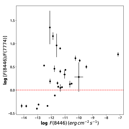
Figure 2: Log-Log plot of F($\lambda$8446)/F($\lambda$7774) vs F($\lambda$8446): The error bars are indicated. In 77% cases, F($\lambda$8446) $>$ F($\lambda$7774).

4.1.2 Collisional Excitation

Bhatia & Kastner (1995) built a hybrid model to compute the collisionally excited level populations and line intensities of neutral oxygen under optically thin conditions. The intensities of all possible allowed and forbidden O i lines in ultraviolet, visible and infrared wavelength regions were calculated over a range of densities and temperatures seen in astrophysical systems. Kastner & Bhatia (1995) estimated the expected values of $\frac{F(8446)}{F(7774)}$ for various temperature, density combinations for collisional excitation. In the magnetospheric accretion models for HAeBe stars (e.g. Muzerolle et al., 2004), most of the emission lines observed in the visible and near-IR wavelengths are formed in magnetospheric accretion columns. It is possible that O i lines also form in these accretion columns. The typical accretion rates for HAeBe stars are in the range of 1.0$\times$10^-8 – 1.0$\times$10^-6 M_⊙ yr^-1 with a median value of $\sim$2.0$\times$10^-7 M_⊙ yr^-1 (e.g. Mendigutía et al., 2011, 2012). The corresponding density of accretion columns are in the range of 10¹¹ – 10¹³ cm^-3 for temperatures of 6000 – 10000 K, for typical parameters of magnetospheric accretion models (see Muzerolle et al., 2004, 1998, 2001; Hartmann et al., 1994). We have taken theoretical O i line flux ratio values corresponding to these temperature, density combinations from Kastner & Bhatia (1995). Observational data is shown in Figure 3 for 50 HAeBe stars, including the measurements of 30 sources from Fairlamb et al. (2017). The flux values of O i $\lambda$7774 and $\lambda$8446 corresponding to a temperature of 5000 K and densities of 10¹⁰, $10^{11}$, $10^{12}$ cm^-3 are represented as dotted lines in Figure 3 and $T$ = 10,000 K, n_e = 10¹⁰, 10¹¹, 10¹² cm^-3 combinations are shown in dashed lines. Figure 3 shows that the observed flux ratio for almost all the sources in our sample is greater than those predicted for densities $>$ 10¹¹ cm^-3. Additionally, models for H$\alpha$ emission in HBe stars also require densities of n_e = 2$\times$10¹² cm^-3 for the line forming region (see Patel et al., 2016, 2017). Although these studies do not discuss about O i line forming region, the strong correlation between H$\alpha$ and O i line emission (see Section 4.1.4) indicates that both lines are formed in the same region. Thus, our analysis suggest that collisional excitation may not be the prominent mechanism at densities $>$ 10¹¹ cm^-3 seen in the line forming regions of HAeBe stars.

We have included O i $\lambda$ $\lambda$7774, 8446 line measurements of a sample of HAeBe stars studied in Fairlamb et al. (2017). These objects were observed with X-shooter spectrograph mounted at Very Large Telescope, Chile. Figure 3 shows that the inclusion of the sample of HAeBe stars from X-Shooter provides more data in the lower flux regime of 7774 and 8446 lines. Further, O i $\lambda$8446 flux values are more intense than the theoretical estimates corresponding to $T$ = 5000/10000 K and n_e = $10^{11}$ cm^-3. This analysis strengthens the claim that collisional excitation is not the dominant excitation mechanism for the production of O i emission lines in HAeBe stars.

Further confirmation is obtained from the analysis of the infrared spectra of HAeBe stars. It has been proposed that if collisional excitation is the dominant excitation mechanism, the equivalent width of $\lambda$13165 should be greater than that of $\lambda$11287 i.e., $W(13165)/W(11287)\geq 1$ at T = 10,000 and 20,000 K, respectively, for n_e = 10¹⁰ – 10¹² cm^-3 (Bhatia & Kastner, 1995). For most of our sample of stars we found that the emission line strength of O i $\lambda$11287 higher than that of $\lambda$13165 (see Figure 4), confirming that collisional excitation does not play a major role in the formation of O i emission lines in HAeBe stars.

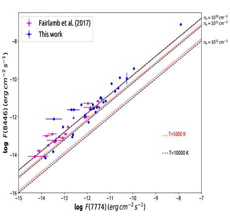
Figure 3: Log-Log plot of F(8446) vs. F(7774): red dotted lines correspond to theoretical flux values for T = 5000 K and black dashed lines correspond to T = 10000 K, for n_e = 10¹⁰, 10¹¹, 10¹² cm^-3 (Kastner & Bhatia, 1995). The sources from Fairlamb et al. (2017) are shown in purple triangles.

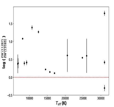
Figure 4: Plot of ratio of EWs of O i $\lambda$11287 to O i $\lambda$13165 against effective temperature of the star. It can be seen that in most cases $\frac{EW({11287})}{EW({13165})}>$1.

4.1.3 Continuum fluorescence

Continuum fluorescence was invoked as the excitation mechanism for the production of O i lines in the spectra of planetary nebulae (Seaton, 1968) and Orion Nebula (Grandi, 1975b). Grandi in his thesis (Grandi, 1975a) and in a paper summarizing the thesis results (Grandi, 1975b) showed that the expected theoretical ratio of the line strengths of the $\lambda$13165 and $\lambda$11287 lines due to starlight excitation (equivalently continuum fluorescence) should be of the order of 10 or slightly more. These model predictions are summarized in Tables 7 and Table 2 of Grandi (1975a) and Grandi (1975b) respectively and also described in the text. In essence, $\lambda$13165 is predicted to be much stronger than $\lambda$11287 if continuum fluorescence is the dominant excitation mechanism for the O i lines (also see Strittmatter et al., 1977). This prediction by Grandi was confirmed observationally for the Orion nebula in the spectroscopic studies by Lowe, Moorhead & WehlauLowe (1977). Also, strong O i emission lines at 7002 Å, 7254 Å and 7990 Å lines would be observed in the spectra (Strittmatter et al., 1977; Grandi, 1980). Apart from the Orion nebula, another instance where the $\lambda$13165 line is stronger than the $\lambda$11287 line is in the inner 10 arcsecond sized nebula surrounding P Cygni. Near-infrared 1$-$2.5 micron spectra by Smith & Hartigan (2006) of this region gives a value of 2.55$\pm$0.57 for the ratio of the 13165 & 11287 line strengths.

Our analysis show that the emission strength of O i $\lambda$11287 is greater than that of O i $\lambda$13165 for our sample of HAeBe stars (Figure 4). In addition, we do not see emission lines at 7002 Å, 7254 Å and 7990 Å in any of the object spectra. This suggests that continuum fluorescence is unlikely to be the dominant mechanism for the formation of O i emission lines in HAeBe stars.

4.1.4 Lyman $\beta$ fluorescence

Lyman $\beta$ (Ly$\beta$) fluorescence occurs because the $3d^{3}D^{0}$ level of O i is populated by Ly$\beta$ radiation, with subsequent cascades producing the O i $\lambda\lambda$11287, 8446, 1304 lines in emission (Figure 5). This is due to the near coincidence in wavelength of Lyman beta and the O i resonance line 2$p~{}^{3}P_{2}$ – 3$d~{}^{3}D^{0}_{321}$ at 1025.77 Å (Bowen, 1947). Our analysis show that the cascade lines expected from Ly$\beta$ fluorescence, O i $\lambda$8446 and O i $\lambda$11287 are quite strong in the spectra of HAeBe stars. Also, O i $\lambda$7774 is less intense than O i $\lambda$8446, suggesting that collisional excitation and recombination are relatively less important for O i excitation in HAeBe stars. Similarly, the lower emission strength of O i $\lambda$13165 with respect to $\lambda$11287 rules out collisional excitation and continuum fluorescence as the dominant mechanisms for the production of O i lines. Further, O i $\lambda\lambda$7002, 7254, 7990 emission lines are not present in the spectra of HAeBe stars. These lines are generally seen in sources where O i lines are excited by continuum fluorescence. All these pieces of evidence strongly suggest that Ly$\beta$ fluorescence is likely to be the dominant excitation mechanism for the production of O i lines in HAeBe stars.

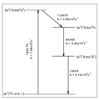
Figure 5: Figure shows the pumping and the fluorescent transitions in O i caused by the Lyman beta fluorescence process.

If Ly$\beta$ fluorescence is responsible for O i emission in HAeBe stars, then one would expect a correlation between H$\alpha$ and O i $\lambda$8446 line intensities. Ly$\beta$ photon results from the n = 3$-$1 transition of the hydrogen atom and the H$\alpha$ photon results from the transition n = 3$-$2. Thus the upper level of both the transitions are the same. In other words, hydrogen atoms in the excited state of n = 3 are responsible for both lines. If these lines originate from the same gas component, one would expect their intensities to be correlated. If, in addition, O i $\lambda$8446 intensity is proportional to Ly$\beta$ intensity, then one would expect a correlation between H$\alpha$ and O i $\lambda$8446. This is shown in Figure 6, where F($\lambda$8446) is shown as a function of F(H$\alpha$) for our sample and those from Fairlamb et al. (2017). A correlation in seen between the flux values of H$\alpha$ and O i $\lambda$8446, suggesting the application of Ly$\beta$ fluorescence process. A linear fit to the distribution of points in Figure 6 gives a relation of the form F($\lambda$8446)$\propto$F(H$\alpha$)^1.02±0.04, with a Pearson’s correlation coefficient of 0.96. From the analysis it is clear that H$\alpha$ emission is correlated with the emission strength of O i $\lambda$8446. This particularly has implications in understanding the region of formation of O i emission lines in HAeBe stars.

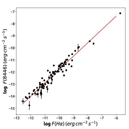
Figure 6: Log-Log plot of F(8446) vs F(H$\alpha$): The sample of HAeBe stars from our studies and from Fairlamb et al. (2017) are shown in black circles. We plotted 97 sources including 57 from Fairlamb et al. (2017), of which 7 are common between Fairlamb et al. (2017) and our sample.

If Ly$\beta$ photons and O i atoms do not co-exist, Ly$\beta$ fluorescence would not have been possible since Ly$\beta$ gets scattered off neutral hydrogen resulting in the production of Ly$\alpha$ and H$\alpha$, before interacting with neutral oxygen atoms. This is the reason why Ly$\beta$ fluorescence does not operate in Orion nebula where Ly$\beta$ photons are trapped in the inner regions of the nebula whereas the O i is confined in the exterior (Grandi, 1975b). In the case of HAeBe stars, H$\alpha$ is thought to originate in the magnetospheric accretion columns which connects the inner disk to the central star. The fact that Ly$\beta$ fluorescence operates in HAeBe stars suggests that O i emission lines are also formed in these accretion columns in HAeBe stars.

It is worth noting that the gas has to be optically thick in H$\alpha$ in order for O i $\lambda$8446 to get excited by Ly$\beta$ fluorescence. From the equations of level populations in statistical equilibrium, Grandi (1980) derived an optical depth in H$\alpha$ ($\tau_{H\alpha}$) of 2000, considering Ly$\beta$ fluorescence operating in active galaxies. We examined whether the line forming region in HAeBe stars are optically thick in H$\alpha$. For the sample of HAeBe stars considered in this study, the median flux ratio F(H$\alpha$/$\lambda$8446)_obs is 65.2. From the analysis of level populations, Strittmatter et al. (1977) derived a theoretical H$\alpha$ to O i $\lambda$8446 flux ratio of around 7500, under optically thin conditions. The optical depth of H$\alpha$ can be estimated from the ratio of theoretical to observed line flux ratio, i.e., $\tau_{H\alpha}$ = 7500 / F(H$\alpha$/$\lambda$8446)_obs = 115. The sufficiently high value of optical depth in H$\alpha$ derived in the case of HAeBe stars agrees with the assumption that the gas needs to be optically thick thereby trapping the Lyman beta photons, paving way for Ly$\beta$ fluorescence.

5 Conclusion

From an analysis of the observed optical spectra of 62 HAeBe stars and near-infrared spectra of 17 HAeBe stars, we have shown that Ly$\beta$ fluorescence is likely to be the dominant excitation mechanism for the formation of O i emission lines. We ruled out recombination and continuum fluorescence as the possible excitation mechanisms as the emission strength of O i $\lambda$8446 and $\lambda$11287 are much stronger than the adjacent O i lines at $\lambda$7774 and $\lambda$13165, respectively. We found that collisional excitation does not contribute substantially to O i emission from the comparative analysis of the observed line flux values of $\lambda$7774 and $\lambda$8446 with those predicted by the theoretical models of Kastner & Bhatia (1995).

References

- Ashok et al. (2006) Ashok, N. M., Banerjee, D. P. K., Varricatt, W. P., Kamath, U. S. 2006, MNRAS, 368, 592
- Banerjee & Ashok (2012) Banerjee, D. P. K., Ashok, N. M. 2012, BASI, 40, 243
- Bessell (1983) Bessell, M. S. 1983, PASP, 95, 480
- Bhatia & Kastner (1995) Bhatia, A. K., Kastner, S. O. 1995, ApJS, 96, 325
- Bowen (1947) Bowen, I. S. 1947, PASP, 59, 196
- Briot (1981) Briot, D. 1981, A&A, 103, 5
- Cohen & Kuhi (1979) Cohen, M., Kuhi, L. V. 1979, ApJS, 41, 743
- Calvet & Gullbring (1998) Calvet, N., Gullbring, E. 1998, ApJ, 509, 802
- Carmona et al. (2010) Carmona, A., van den Ancker, M. E., Audard, M., et al. 2010, A&A, 517, A67
- Castelli et al. (1997) Castelli, F., Gratton, R. G., Kurucz, R. L. 1997, A&A, 318, 841
- Cauley & Johns-Krull (2015) Cauley, P. W. & Johns-Krull, C. M. 2015, ApJ, 810, 5
- Corcoran & Ray (1998) Corcoran, M., Ray, T. P. 1998, A&A, 331, 147
- Dahm (2008) Dahm, S. E. 2008, AJ, 136, 521
- Drew et al. (1997) Drew, J. E., Busfield, G., Hoare, M. G., et al. 1997,MNRAS, 286, 538
- Fairlamb et al. (2017) Fairlamb, J. R., Oudmaijer, R. D., Mendigutia, I. et al. 2017, MNRAS, 464, 4721
- Fairlamb et al. (2015) Fairlamb, J. R., Oudmaijer, R. D., Mendigutia, I. et al. 2015, MNRAS, 453, 976
- Fang et al. (2009) Fang, M., van Boekel, R., Wang, W. et al. 2009, A&A, 504, 461
- Felenbok et al. (1988) Felenbok, P., Czarny, J., Catala, C., Praderie, F. 1988, A&A, 201, 247
- Ferland & Netzer (1979) Ferland, G., Netzer, H. 1979, ApJ, 229, 274
- Finkenzeller & Mundt (1984) Finkenzeller, U., Mundt, R. 1984, A&AS, 55, 109
- Gandolfi et al. (2008) Gandolfi, D., Alcalá, J. M., Leccia, S. et al. 2008, ApJ, 687, 1303
- Garrison (1970) Garrison, R. F. 1970, AJ, 75, 1001
- Gorti & Bhatt (1993) Gorti, U., Bhatt, H. C. 1993, A&A, 270, 426
- Grandi (1975a) Grandi, S. A. 1975a, Ph.D. thesis, Univ. Arizona
- Grandi (1975b) Grandi, S. A. 1975b, ApJ, 196, 465
- Grandi (1980) Grandi, S. A. 1980, ApJ, 238, 10
- Gullbring et al. (1998) Gullbring, E., Hartmann, L., Briceno, C., Calvet, N. 1998, ApJ, 492, 323
- Hamann & Persson (1992) Hamann, F., Persson, S. E. 1992, ApJS, 82, 247
- Hartmann et al. (1994) Hartmann, L., Hewett, R., Calvet, N. 1994, ApJ, 426, 669
- Hauschildt et al. (1999) Hauschildt, P. H., Allard, F., Baron, E. 1999, ApJ, 512, 377
- Herbig (1960) Herbig G. H., 1960, ApJS, 4, 337
- Herczeg & Hillenbrand (2008) Herczeg, G. J. & Hillenbrand, L. A. 2008, ApJ, 681, 594
- Hernandez et al. (2004) Hernández, J., Calvet, N., Briceño, C. et al. 2004, AJ, 127, 1682
- Hillenbrand et al. (1992) Hillenbrand, L. A., Strom, S. E., Vrba, F. J., Keene, J. 1992, ApJ, 397, 613
- Ingleby et al. (2013) Ingleby, L., Calvet, N., Herczeg, G. et al. 2013, ApJ, 767, 112
- Kastner & Bhatia (1995) Kastner, S. O., & Bhatia, A. K. 1995, ApJ, 439, 346
- Kenyon & Hartmann (1995) Kenyon, S. J., Hartmann, L. 1995, ApJS, 101, 117
- Kurucz (1993) Kurucz R. 1993, ATLAS9 Stellar Atmosphere Programs and 2 km/s grid, Kurucz CD-ROM No. 13. Smithsonian Astrophysical Observatory, Cambridge, MA
- Lee & Chen (2007) Lee, H.-T., & Chen, W. P. 2007, ApJ, 657, 884
- Liu et al. (2011) Liu, T., Zhang, H. Wu, Y. et al. 2011, ApJ, 734, 22
- Lowe, Moorhead & WehlauLowe (1977) Lowe, R. P., Moorhead, J. M., Wehlau, W. H. 1977, ApJ, 214, 712
- Manoj et al. (2006) Manoj, P., Bhatt, H. C., Maheswar, G., Muneer, S. 2006, ApJ, 653, 657
- Mathew et al. (2012a) Mathew, B., Banerjee, D. P. K., Naik, S., Ashok, N. M., 2012a, MNRAS, 423, 2486
- Mathew et al. (2012b) Mathew, B., Banerjee, D. P. K., Subramaniam, A., Ashok, N. M., 2012b, ApJ, 753, 13
- McDonald et al. (2017) McDonald, I., Zijlstra, A. A., & Watson, R. A. 2017, VizieR Online Data Catalog, 747,
- Mora et al. (2001) Mora, A., Merín, B., Solano, E., et al. 2001, A&A, 378, 116
- Mathis (1990) Mathis, J. S. 1990, ARA&A, 28, 37
- Mendigutía et al. (2011) Mendigutía, I., Calvet, N., Montesinos, B. et al. 2011, A&A, 535, A99
- Mendigutía et al. (2012) Mendigutía I., Mora A., Montesinos B. et al. 2012, A&A, 543, A59
- McClure (2009) McClure, M. 2009, ApJ, 693, L81
- Munari et al. (2005) Munari, U., Sordo, R., Castelli, F., & Zwitter, T. 2005, A&A, 442, 1127
- Muzerolle et al. (2004) Muzerolle, J., D’Alessio, P., Calvet, N., & Hartmann, L. 2004, ApJ, 617, 406
- Muzerolle et al. (2001) Muzerolle, J., Calvet, N., Hartmann, L. 2001, ApJ, 550, 944
- Muzerolle et al. (1998) Muzerolle, J., Calvet, N., Hartmann, L. 1998, ApJ, 492, 743
- Patel et al. (2017) Patel, P., Sigut, T. A. A., Landstreet, J. D. 2017, ApJ, 836, 214
- Patel et al. (2016) Patel, P., Sigut, T. A. A., Landstreet, J. D. 2016, ApJ, 817, 29
- Pecaut & Mamajek (2013) Pecaut, M. J., Mamajek, E. E. 2013, ApJS, 208, 9
- Porter & Rivinius (2003) Porter, J. M., & Rivinius, T. 2003, PASP, 115, 1153
- Seaton (1968) Seaton, M. J. 1968, MNRAS, 139, 129
- Shu et al. (1994) Shu, F., Najita, J., Ostriker, E. et al. 1994, ApJ, 429, 781
- Slettebak (1951) Slettebak, A. 1951, ApJ, 113, 436
- Smith & Hartigan (2006) Smith, N., Hartigan, P. 2006, ApJ, 638, 1045
- Skiff (2014) Skiff, B. A. 2014, VizieR Online Data Catalog, 1,
- Strittmatter et al. (1977) Strittmatter, P. A., Woolf, N. J., Thompson, R. I. et al. 1977, ApJ, 216, 23
- The et al. (1994) The, P. S., de Winter, D., Perez, M. R. 1994, A&AS, 104, 315
- Tjin A Djie et al. (2001) Tjin A Djie, H. R. E., van den Ancker, M. E., Blondel, P. F. C. et al. 2001, MNRAS, 325, 1441
- Vieira et al. (2003) Vieira, S. L. A., Corradi, W. J. B., Alencar, S. H. P. et al. 2003, AJ, 126, 2971
- Waters & Waelkens (1998) Waters L. B. F. M., Waelkens, C., 1998, ARA&A, 36, 233
- Zhong et al. (2015) Zhong, J., Lépine, S., Li, J. et al. 2015, Research in Astronomy and Astrophysics, 15, 1154
- Zacharias et al. (2004) Zacharias, N., Monet, D. G., Levine, S. E. et al. 2004, Bulletin of the American Astronomical Society, 36, 48