Indirect strong coupling regime between a quantum dot and a nanocavity mediated by a mechanical resonator

Abstract

Achieving strong coupling between light and matter is usually a challenge in Cavity Quantum Electrodynamics (cQED), especially in solid state systems. For this reason is useful taking advantage of alternative approaches to reach this regime, and then, generate reliable quantum polaritons. In this work we study a system composed of a quantized single mode of a mechanical resonator interacting linearly with both a single mode nanocavity and a two-level single quantum dot. In particular, we focus on the behavior of the indirect light-matter interaction when the phonon mode interfaces both parts. By diagonalization of the Hamiltonian and computing the density matrix in a master equation approach, we evidence several features of strong coupling between photons in optical cavities and excitons in a quantum dot. For large energy detuning between the cavity and the mechanical resonator it is obtained a phonon-dispersive effective Hamiltonian which is able to retrieve much of the physics of the conventional Jaynes-Cummings model (JCM). In order to characterize this mediated coupling, we make a quantitative comparison between both models and analyze light-matter entanglement and purity of the system leading to similar results in cQED.

1 Introduction

In the last decades solid state systems have been widely used as a platform to interface light with matter in the cavity quantum electrodynamics (cQED) frame [19, 15, 14] which opens the route towards quantum computation and quantum information processing devices [20]. Different regimes of light-matter interaction have been studied and each of them are useful to play some role in current technologies. On the one hand, weak coupling between light and matter can be used to generate single-photons on-demand; on the other hand, strong coupling regime is exploited to transfer quantum information between light and matter and perform quantum logic operations. Additionally, the control over the light-matter interaction rate and the spontaneous emission decay are a desired feature in order to achieve versatility and efficiency.

Since quantum dot-microcavity strong coupling is difficult to achieve in many cQED systems due to fabrication issues and incoherent processes [23, 37], it is really useful taking advantage of other mechanisms that allow to reach this regime. Mechanical modes of semiconductor structures and surface acoustic waves (SAW) are now used to handle the properties of quantum dots embedded in optical microcavities [18, 21]. Usually, the interaction of quantized mechanical modes [27] with quantum dots and optical cavities are modeled with electron-phonon Hamiltonian [34, 36] and optomechanical Hamiltonian [17, 1], respectively. Large optomechanical coupling rates and photon-phonon strong coupling regime have been achieved in different systems, particularly in photonic crystals and micropillars [5, 4]. Besides, active media have been used to enhance optomechanical coupling [22, 13, 26].

Furthermore, it is well known that linear coupling between cavity and mechanical resonators raises in the so-called resolved sideband regime [31, 1, 9], i.e., when phonon energy is larger than the cavity decay rate ($\omega_{m}>\kappa$), in that regime the cavity is pumped by a large coherent field. In addition, there has been recently proposed a coherent field-mediated emitter-phonon linear coupling produced by variations of the spatial distributions of the cavity field [3, 35]. The aim of this work is to study alternative models in polariton cavity optomechanics, different from the standard hybrid optomechanical Hamiltonians in the dispersive regime [25, 16, 24, 33, 38]. This alternative way is exploited to obtain enhancement of light-matter coupling rate and its quantum features such as entanglement which is a key resource for quantum information operations [11, 2, 30, 29]. However, other scenarios involving acoustic phonons show a detrimental impact on the light-matter strong coupling and its effects [7, 10].

The rest of the paper is organized as follows, in section 2 we set the theoretical model for the tripartite cavity-emitter-mechanics system. Then, in section 3, by diagonalization of the Hamiltonian we discuss the possibility of achieving strong coupling regime mediated by phonons and study the dispersive limit of the Hamiltonian. In section 4, using the density operator in the steady state we quantify light-matter entanglement and linear entropy, and show the tomography in different important situations. Finally, in section 5 we make and overview and conclude.

2 Theoretical framework

As stated above, the tripartite system in Figure 1 is typically modeled with optomechanical and electron-phonon dispersive interactions. However, we will alternatively use an approximate Hamiltonian; linear coupling between different parts of the system as is justified in the appendix A. Here, we do not consider light-matter interactions directly. Thus, the Hamiltonian is:

$$\hat{H}=\hat{H}_{0}+\hat{H}_{int}$$ (1)

with

$$\hat{H}_{0}=\hbar\omega_{c}\hat{a}^{\dagger}\hat{a}+\hbar\omega_{a}\hat{\sigma}^{\dagger}\hat{\sigma}+\hbar\omega_{m}\hat{b}^{\dagger}\hat{b},$$ (2)

and

$$\hat{H}_{int}=\hbar g_{cm}\left(\hat{a}\hat{b}^{\dagger}+\hat{a}^{\dagger}\hat{b}\right)+\hbar g_{am}\left(\hat{\sigma}\hat{b}^{\dagger}+\hat{\sigma}^{\dagger}\hat{b}\right).$$ (3)

$\omega_{c}$, $\omega_{a}$ and $\omega_{m}$ are the cavity, exciton recombination and mechanical frequencies, respectively. $\hat{a}$ ($\hat{a}^{\dagger}$) and $\hat{b}$ ($\hat{b}^{\dagger}$) are the annihilation (creation) bosonic operators for photons and phonons, respectively. $\hat{\sigma}=\ket{G}\bra{X}$ is the atomic ladder operator for the two-level system (TLS). The parameters $g_{cm}$ and $g_{am}$ are the optomechanical coupling strength and the atom-phonon coupling strength, respectively.

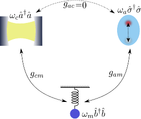
Figure 1: Sketch of the hybrid cQED-optomechanical system [25]. Linear coupling is assumed between the nanocavity and the mechanical resonator, and also between the single-exciton quantum dot and the mechanical resonator. Throughout this work there is no direct interaction between the nanocavity and the quantum dot.

Losses and decoherence arise in the system when it is affected by its environment. These are effectively considered in a master equation approach for the density operator in the Markov approximation [32, 28]:

$$\frac{d\hat{\rho}}{dt}=\frac{i}{\hbar}\left[\hat{\rho},\hat{H}\right]+\kappa\mathcal{L}_{\hat{a}}(\hat{\rho})+P_{X}\mathcal{L}_{\hat{a}^{\dagger}}(\hat{\rho}),$$ (4)

where $\kappa$ is the cavity decay rate and $P_{x}$ is an incoherent excitation to the quantum dots. The Lindblad term for the operator representing a dissipative channel, $\hat{C}$, is defined as $\mathcal{L}_{\hat{C}}(\hat{\rho})=\hat{C}\hat{\rho}\hat{C}^{\dagger}-\frac{1}{2}\hat{C}^{\dagger}\hat{C}\hat{\rho}-\frac{1}{2}\hat{\rho}\hat{C}^{\dagger}\hat{C}$.

Throughout this work, we assume high mechanical coupling rates, $g_{am}/\omega_{a}\approx g_{cm}/\omega_{c}>10^{-3}$, which could be obtained taking advantage of large coherent driven as is shown in the appendix A. While mechanical frequencies considered here are very out of resonance with cavity frequencies ($\omega_{m}/\omega_{c}\sim 10^{-3}$), cavity and exciton recombination frequencies are close each other, i.e. $|\Delta|=|\omega_{a}-\omega_{c}|<g_{am}$. Assuming realistic parameters of the Microcavity Quantum Electrodynamics ($\mu$cQED), $\omega_{c}\approx\omega_{a}\approx 1000meV$, such that $g_{cm}\approx g_{am}\sim meV$. From here on, all frequencies are given in $meV$, assuming $\hbar=1$.

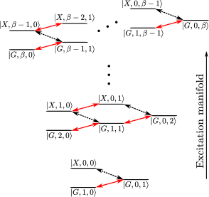
Figure 2: States ladder of the Hamiltonian. Black-dashed arrows represent exciton-phonon interactions ($g_{am}$) and the red ones correspond to photon-phonon interactions ($g_{cm}$). A $\beta$-excitation manifold has $2\beta+1$ states $\{\left|G,\beta-k,k\right>,\left|X,\beta-k-1,k\right>\}$, $k=0,1,...,\beta-1$.

3 Indirect light-matter strong coupling regime

Strong coupling between quantum dots and optical cavities is a hard feature to achieve; usually it requires high control in the positioning of QD inside the cavity, small field modal volume and high quality factor. However, indirect mechanics can be harnessed to reach the vacuum Rabi splitting regime. We consider a quantized mechanical mode interacting simultaneously with both the cavity and QD in a linear way according to equation (3). Since the Hamiltonian commutes with the total number operator ($N=\hat{a}^{\dagger}\hat{a}+\hat{\sigma}^{\dagger}\hat{\sigma}+\hat{b}^{\dagger}\hat{b}$), then it can be diagonalized for each excitation manifold as shown in Figure 2.

By numerical diagonalization of the Hamiltonian in a large energy detuning regime between cavity (emitter) and mechanical oscillator, is found that the eigenstates of the system are separable in a polariton state and a phonon Fock state: $\left|\psi_{n}^{\ell}\right>\approx\left|n\pm\right>\otimes\left|\ell\right>$. From here on, polariton in this context will be understood as a phonon-induced polariton (PIP). Moreover, similarly to the Jaynes-Cummings model, the dispersion diagram exhibits anticrossing between two dressed states; the upper and lower polaritons, $\left|n+\right>\otimes\left|\ell\right>$ and $\left|n-\right>\otimes\left|\ell\right>$. Each polariton is a superposition of light-matter bare states: $\left|n\pm\right>=\cos{\theta_{n}}\left|G,n\right>\pm\sin{\theta_{n}}\left|X,n-1\right>$, where $\theta_{n}$ depends on the system parameters and photon number. This situation is illustrated in the Figure 3 for the third-excitation manifold.

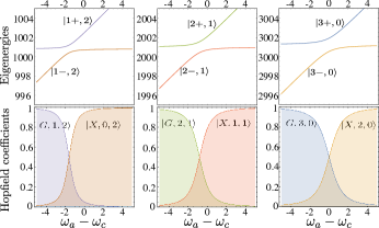
Figure 3: Numerical diagonalization of the Hamiltonian for the third- excitation manifold. The trivial phonon eigenstate is the bare state $\left|G,0,3\right>$ with eigenenergy $\omega_{m}$ (not shown here). Parameters: $g_{cm}=g_{am}=20$, $\omega_{m}=1$ and $\omega_{c}=1000$.

In the limit of large cavity-photon detuning [6], ($|\Delta_{c}|=|\omega_{c}-\omega_{m}|\gg 1$), and emitter-cavity resonance ($\omega_{a}=\omega_{c}$), as is derived in the appendix B, it can be obtained an effective Jaynes-Cummings Hamiltonian:

$$\hat{H}_{eff}=\frac{g_{cm}^{2}}{\Delta_{c}}\hat{a}^{\dagger}\hat{a} + \frac{g_{am}^{2}}{\Delta_{c}}\hat{\sigma}^{\dagger}\hat{\sigma}+\left(\frac{g_{am}^{2}}{\Delta_{c}}\sigma_{z}-\frac{g_{cm}^{2}}{\Delta_{c}}\right)\hat{b}^{\dagger}\hat{b}$$ (5)

$$\frac{g_{cm}g_{am}}{\Delta_{c}}\left(\hat{a}\hat{\sigma}^{\dagger}+\hat{a}^{\dagger}\hat{\sigma}\right).$$

This Hamiltonian is block-diagonal respect to the phonon number and for each one, $\left<\ell\right|H_{eff}\left|\ell\right>$ is a block-diagonal matrix respect to the polaritonic excitation manifold, $\{\left|G,n\right>,\left|X,n-1\right>\}$, in a similar way that the standard Jaynes-Cummings Hamiltonian:

$$\hat{H}_{eff}=\begin{pmatrix}\frac{g_{cm}^{2}}{\Delta_{c}}n-\frac{g_{am}^{2}}{\Delta_{c}}\ell&\frac{g_{cm}g_{am}}{\Delta_{c}}\sqrt{n}\\ \frac{g_{cm}g_{am}}{\Delta_{c}}\sqrt{n}&\frac{g_{cm}^{2}}{\Delta_{c}}(n-1)-\frac{g_{am}^{2}}{\Delta_{c}}(\ell+1)\end{pmatrix}$$ (6)

By diagonalization of the previous matrix, it is obtained some useful relations. For each pair of upper/lower phonon-induced polaritons the anticrossing arises in $\omega_{a}-\omega_{c}=\bar{g}_{m}\ell$ where

$$\bar{g}_{m}=\frac{g_{am}^{2}+g_{cm}^{2}}{\omega_{a}-\omega_{m}}$$ (7)

is the effective light-matter coupling strength. The splitting at resonance is

$$\lambda_{+}-\lambda_{-}=\frac{g_{cm}^{2}}{\Delta_{c}}\sqrt{1+\epsilon^{4}(1+2\ell)^{2}+2\epsilon(2n-2\ell-1)},$$ (8)

where $\epsilon=g_{am}/g_{cm}$ is the ratio between the mechanical interaction rates. Moreover, in the anticrossing region, $\ell=0$ and $\epsilon=1$, the splitting between upper and lower polaritons is $\bar{g}_{m}\sqrt{n}$ in analogy with the Jaynes-Cummings case.

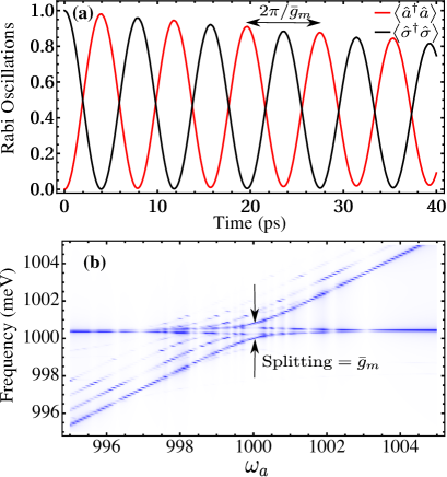
Figure 4: Vacuum Rabi Splitting. (a) Mean number of photons (Red line) and matter excitations (Black line). They display damped Rabi oscillations with frequency $\bar{g}_{m}$. (b) Cavity light-emitted spectrum computed by means of the Green function method [8]. The spectrum is normalized to unity in order to show other optical transitions. A splitting of $\bar{g}_{m}$ is obtained. Parameters: $g_{cm}=g_{am}=20$, $\omega_{c}=1000$, $\omega_{m}=1$, $\kappa=10^{-2}$ and $P_{X}=10^{-3}$. Time units $meV^{-1}/\hbar\approx 1.5^{-1}ps$.

Summarizing, the Hamiltonian proposed (Equation (1)) allows a major control on the effective light-matter coupling strength, e.g., by increasing the mechanical interaction rates or decreasing the cavity (exciton) energy, the splitting could become larger than the spectral linewidths, i.e., $\bar{g}_{m}>\kappa$. Hence, the emission exhibits Vacuum Rabi splitting showing a quantum coherent exchange of particles between the nanocavity and the quantum dot, which gives a first feature of strong coupling regime. We can observe this behavior in the mean number of photons and matter excitations since they display Rabi oscillations (Figure 4a), and also in the photoluminescence spectrum which is defined as follows:

$$S_{a}(\omega,t)=\frac{1}{\pi\left<a^{\dagger}a\right>}Re\int_{0}^{\infty}e^{-i\omega\tau}\left<a^{\dagger}(t+\tau)a(t)\right>d\tau.$$ (9)

Emission cavity spectrum shown in Figure 4b exhibits single-polariton optical transitions for each phonon number, i.e., $\ket{1\pm,\ell}\rightarrow\ket{G,0,\ell}$. Optical transitions involving higher polaritons are not present because the excitonic pumping is not enough to rise in the states ladder.

4 Light-matter entanglement

Even though vacuum Rabi splitting is a first signature of quantum polaritons, it is necessary to find other physical properties such as light-matter entanglement, non-classical photon statistics, etc. in order to herald genuine quantum polaritons. In this section we focus on a low excitation regime, $\kappa>P_{X}$, to explore single-polariton properties when it is induced by phonons. First of all, we quantify the entanglement between cavity and emitter by computing negativity, which is defined as $\mathcal{N}=2\sum_{\lambda<0}|\lambda|$, where $\lambda$ denotes all the eigenvalues of the partial transpose of the density matrix $\hat{\rho}$ [11]. However, before doing this, a partial trace is carried out on the phonon mode, $\hat{\rho}^{red}=\sum_{\ell}\bra{\ell}\hat{\rho}\ket{\ell}$. The results are shown in Figure 5. Additionally, the linear entropy, given by $S_{L}=1-Tr(\hat{\rho}^{2})$, is computed in order to compare the purity of the state with the entanglement.

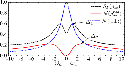
Figure 5: Linear entropy and negativity in the steady state. Parameters: $g_{cm}=g_{am}=20$, $\omega_{c}=1000$, $\omega_{m}=1$, $\kappa=10^{-2}$ and $P_{X}=10^{-3}$. Parameters indicated as $\Delta_{1}$ and $\Delta_{2}$ correspond to the maximum values of linear entropy and negativity, respectively.

As shown in Figure 5, when dissipation affects the system, entanglement is not maximum at resonance in comparison with the Hamiltonian case where a polariton state, which in our case is induced by phonons, becomes a Bell state and therefore, maximally entangled. However, Because of the competition between the mechanical interaction and dissipative effects, entanglement is found to be maximum out of resonance. This phenomenology appears also in the Jaynes-Cummings model [29]. Figure 5 also shows that linear entropy has a local minimum when entanglement vanishes at resonance. To better understand this, in Figure 6 it is plotted the density matrix in some key points indicated in Figure 5: at resonance; $\Delta=0$ (Figure 6a), at maximum of the linear entropy; $\Delta=1.1$ (Figure 6b), at maximum of the negativity; $\Delta=2.75$ (Figure 6c) and for large enough detuning; $\Delta=10$ (Figure 6d).

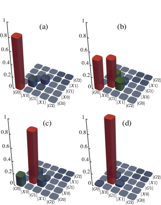
Figure 6: Tomography of the reduced density matrix, $|\rho_{ss}^{red}|$ in the steady state for the parameters indicated in Figure 5. (a) $\Delta=0$, (b) $\Delta=\Delta_{1}=1.1$, (c) $\Delta=\Delta_{2}=2.75$ and (d) $\Delta=10$. Other parameters: $g_{cm}=g_{am}=20$, $\omega_{c}=1000$, $\omega_{m}=1$, $\kappa=10^{-2}$ and $P_{X}=10^{-3}$.

At resonance, because losses are larger than gain, most of the population is carried into the ground state with negligible coherences (non-diagonal elements), i.e., a mostly pure and non-entangled state is obtained, $\ket{G,0}$. When linear entropy becomes maximum, a highly mixed state with large entanglement is found. However, in this regime of parameters ($\kappa>P_{X}$), the best condition to finding simultaneously high purity and high entanglement is in $\Delta=2.75$. Finally, very out of resonance, for both Hamiltonian and dissipative cases, entanglement and linear entropy decrease since the mechanical interaction effect is reduced and the combined effect of pumping and losses bring the system to a pure and non-entangled state $\ket{X,0}$.

Furthermore, we find a high fidelity between the phonon-traced density matrix and the Jaynes-Cummings matrix density with the same dissipative rates ($\kappa$ and $P_{X}$, with $P_{X}/\kappa=10^{-1}$) and Rabi coupling strength $g_{ac}=\bar{g}_{m}/2$, $F=Tr\left[\sqrt{\sqrt{\rho_{ss}^{JC}}\rho_{ss}^{red}\sqrt{\rho_{ss}^{JC}}}\right]\approx 1$. This evidences that polariton induced by phonons is very similar to the conventional polariton arising from JCM.

5 Overview and conclusions

In this work, we have considered a single mechanical mode interacting linearly with a single mode photonic nanocavity and a two-level single-quantum dot. The phonon mode mediates the coupling between photons in the cavity and excitons in the quantum emitter. By exact diagonalization of the Hamiltonian and then taking into account dissipative effects, we find vacuum Rabi splitting arising from mechanical interactions. This means that our model allows achieving indirect light-matter strong coupling regime just for the phonon mediation. Moreover, it was studied the properties of the phonon-induced polariton, which exhibits the same physics of the Jaynes-Cummings model as is demonstrated by derivation of an effective light-matter Hamiltonian valid for large energy detuning between the mechanical resonator and the cavity (or the emitter). Finally, we studied the light-matter entanglement and purity of the state in a low excitation regime ($P_{X}/\kappa=10^{-1}$) in order to find that the condition with strongest quantum properties; large coherences and low mixing degree, is out of resonance ($\Delta=2.75$). At resonance, dissipation overcomes the mechanical effect such that the system goes to the ground state and hence, entanglement vanishes. Moreover, it was found almost perfect fidelity between the single-polariton induced by phonons and standard JC polaritons under the same conditions.

The feasibility of this hybrid platform depends mainly on high mechanical interactions. It could be achieved by a large coherent driven which makes part of the underlying theory to our model. Good candidates to implement the model proposed are the quantum dot-microcavity systems taking advantage of the mechanical modes of semiconductor nanostructures and the advanced field of surface acoustic waves in solid state systems. Furthermore, in Circuit Quantum Electrodynamics, superconducting qubits provide high interaction strengths with nanomechanical resonators.

Appendix A Derivation of the linear cavity-phonon and emitter-phonon Hamiltonian

The ”linearization” of both interaction Hamiltonians (cavity-phonon and emitter-phonon) is a combination of derivations carried out in [1] and in [3]. In standard optomechanics, the quantized resonator displacement [27], $\hat{x}$, modifies the cavity frequency because it changes the length of the cavity. In first approximation,

$$\omega_{c}(x)\approx\omega_{c}(0)+\frac{\partial\omega(x)}{\partial x}\bigg{\rvert}_{x=0}\hat{x}.$$ (10)

The mechanical resonator is modeled by a quantum harmonic oscillator, where the displacement operator, $\hat{x}=x_{ZPF}(\hat{b}^{\dagger}+\hat{b})$, is written in terms of annihilation and creation phonon operator. $x_{ZPF}$ is the zero-point fluctuation amplitude of the mechanical resonator. The optomechanical interaction Hamiltonian is then,

$$\hat{H}_{OM}=\hbar g_{OM}\hat{a}^{\dagger}\hat{a}\left(\hat{b}+\hat{b}^{\dagger}\right),$$ (11)

where $g_{OM}=(\partial\omega/\partial x)x_{ZPF}$. For more detail see Section III in [1]. Now it is considered a laser driving to the cavity which allows separate the cavity field in two compounds, one average coherent amplitude $\bar{\alpha}$ because of the laser driving, and other fluctuating term $\delta\hat{a}$, which is the one we will be interested. By substituting $\hat{a}=\bar{\alpha}+\delta\hat{a}$ in the interaction Hamiltonian, we have

$$\hat{H}_{OM}=\hbar g_{OM}\left[|\bar{\alpha}|^{2}+\bar{\alpha}\delta\hat{a}^{\dagger}+\bar{\alpha}^{*}\delta\hat{a}+\delta\hat{a}^{\dagger}\delta\hat{a}\right]\left(\hat{b}+\hat{b}^{\dagger}\right).$$ (12)

quadratic term in $\delta\hat{a}$ is negligible respect to the other terms accompanied by $\bar{\alpha}$. The quadratic term in $\bar{\alpha}$ is an average radiation pressure that may be omitted by a shift of the displacement’s origin. So, the effective optomechanical Hamiltonian is:

$$\hat{H}_{OM}=\hbar g_{cm}\left(\delta\hat{a}+\delta\hat{a}^{\dagger}\right)\left(\hat{b}+\hat{b}^{\dagger}\right),$$ (13)

where $g_{cm}=g_{OM}\sqrt{\bar{n}_{cav}}$ is the optomechanical coupling strength. The condition $g_{cm}>\kappa$ leads to the strong coupling regime in cavity optomechanics [1, 9, 31].

With regard to the emitter-phonon interaction, the ”linearization” of the Hamiltonian, as is proposed in [3], starts assuming that mechanical resonator does not affect just the frequency cavity but also the emitter-cavity coupling rate,

$$g(x)\approx g(0)+\frac{\partial g(x)}{\partial x}\bigg{\rvert}_{x=0}\hat{x},$$ (14)

such that the light-matter interaction Hamiltonian, using the rotating wave approximation (RWA) and assuming the direct light-matter interaction off ($g(0)$=0) yields,

$$\hat{H}_{int}=\gamma\left(\hat{b}+\hat{b}^{\dagger}\right)\left(\hat{\sigma}^{\dagger}\hat{a}+\hat{\sigma}\hat{a}^{\dagger}\right),$$ (15)

where $\gamma=(\partial g/\partial x)x_{ZPF}$. Again, considering a laser driving to the cavity, we may express the cavity field operator as $\hat{a}=\bar{\alpha}+\delta\hat{a}$ and now the fluctuation terms can be neglected such that this interaction Hamiltonian becomes,

$$\hat{H}_{int}=\hbar g_{am}\left(\hat{\sigma}+\hat{\sigma}^{\dagger}\right)\left(\hat{b}+\hat{b}^{\dagger}\right),$$ (16)

where $g_{am}=\gamma\sqrt{\bar{n}_{cav}}$ is the atom-phonon coupling rate. This mechanics is referred in the literature as an atom-phonon interaction through mode field coupling [3]. In Hamiltonians (13) and (16) the coupling rates can be increased by a driving laser to the cavity since they depend on $\bar{\alpha}=\sqrt{\bar{n}_{cav}}$. Also it can be analyzed the role of the rotating wave approximation in these Hamiltonians.

Appendix B Effective Hamiltonian in a cavity-phonon large detuning

Following an analogous derivation from [6], a phonon dispersive Hamiltonian is obtained valid in a large cavity-phonon energy detuning regime. Starting from the linear Hamiltonian 1 and with a system of unit where $\hbar=1$, we transform the Schrödinger equation to the interaction picture (IP):

$$i\frac{d}{dt}\ket{\Psi_{IP}(t)}=\hat{H}_{IP}\ket{\Psi_{IP}(t)},$$ (17)

by using the unitary operator $\hat{U}=\exp(-i\hat{H}_{0}t)$ over the interaction Hamiltonian:

$$\hat{H}_{IP}=\hat{U}^{-1}\hat{H}_{int}\hat{U}=g_{cm}\left(\hat{a}^{\dagger}\hat{b}e^{i\Delta_{c}t}+\hat{a}\hat{b}^{\dagger}e^{-i\Delta_{c}t}\right)$$

$$+g_{am}\left(\hat{\sigma}^{\dagger}\hat{b}e^{i\Delta_{a}t}+\hat{\sigma}\hat{b}^{\dagger}e^{-i\Delta_{a}t}\right),$$ (18)

where $\Delta_{c}=\omega_{c}-\omega_{m}$ and $\Delta_{a}=\omega_{a}-\omega_{m}$ are the cavity-phonon and emitter-phonon energy detuning, respectively. The formal solution of equation (17) is:

$$\ket{\Psi_{IP}(t)}=\hat{\mathcal{T}}\left[\exp\left(-i\int_{0}^{t}dt^{\prime}\hat{H}_{IP}(t^{\prime})\right)\right]\ket{\Psi_{IP}(0)}$$ (19)

$$=\left(\hat{1}+(-i)A+\frac{(-i)^{2}}{2}B+\cdots\right)\ket{\Psi_{IP}(0)}.$$

In the last part of this equation was made a perturvative expansion and then was taken into account time-ordering integration. The terms in (19) are:

$$A=\int_{0}^{t}dt^{\prime}\hat{H}_{IP}(t^{\prime})$$ (20)

and

$$B=2\int_{0}^{t}dt^{\prime}\hat{H}_{IP}(t^{\prime})\int_{0}^{t^{\prime}}dt^{\prime\prime}\hat{H}_{IP}(t^{\prime\prime}).$$ (21)

Solving these integrals for $H_{IP}$ in equation (18), we have:

$$A=-i\frac{g_{cm}}{\Delta_{c}}\left(\hat{a}^{\dagger}\hat{b}\left(e^{i\Delta_{c}t}-1\right)-\hat{a}\hat{b}^{\dagger}\left(e^{-i\Delta_{c}t}-1\right)\right)$$

$$-i\frac{g_{am}}{\Delta_{a}}\left(\hat{\sigma}^{\dagger}\hat{b}\left(e^{i\Delta_{a}t}-1\right)-\hat{\sigma}\hat{b}^{\dagger}\left(e^{-i\Delta_{a}t}-1\right)\right).$$ (22)

This term can be neglected if the mean excitations, $\innerproduct{\hat{a}^{\dagger}\hat{b}}{\hat{a}^{\dagger}\hat{b}}\approx\sqrt{\innerproduct{\hat{n}_{a}\hat{n}_{b}}{\hat{n}_{a}\hat{n}_{b}}}$ and $\innerproduct{\hat{\sigma}^{\dagger}\hat{b}}{\hat{\sigma}^{\dagger}\hat{b}}\approx\sqrt{\innerproduct{\hat{n}_{\sigma}\hat{n}_{b}}{\hat{n}_{\sigma}\hat{n}_{b}}}$ are not too large, and if $g_{cm}/\Delta_{c}\ll 1$ (and $g_{am}/\Delta_{a}\ll 1$), which is valid for large detuning.

Now neglecting all the terms quadratics in $\frac{g_{am/cm}}{\Delta_{a/c}}$, which are small in comparison with terms $\frac{g_{am/cm}^{2}}{\Delta_{c/a}}$ and $\frac{g_{cm}g_{am}}{\Delta_{c/a}}$, because of the large detuning, the integral $B$ yields

$$(it)^{-1}B= \frac{g_{cm}^{2}}{\Delta_{c}}\left(\hat{a}^{\dagger}\hat{a}-\hat{b}^{\dagger}\hat{b}\right)+\frac{g_{am}^{2}}{\Delta_{a}}\left(\hat{\sigma}^{\dagger}\hat{\sigma}+\hat{\sigma}_{z}\hat{b}^{\dagger}\hat{b}\right)$$ (23)

$$+g_{cm}g_{am}\left(\hat{a}^{\dagger}\hat{\sigma}-\hat{a}\hat{\sigma}^{\dagger}\right)\hat{b}\hat{b}^{\dagger}\left(\frac{1}{\Delta_{a}}-\frac{1}{\Delta{c}}\right)$$

$$+g_{cm}g_{am}\left(\frac{1}{\Delta_{a}}\hat{a}\hat{\sigma}^{\dagger}+\frac{1}{\Delta_{c}}\hat{a}^{\dagger}\hat{\sigma}\right),$$

Rewriting the equation (19) as

$$\ket{\Psi_{IP}(t)}\approx\left(\hat{1}-it\hat{H}_{eff}\right)\ket{\Psi_{IP}(0)},$$ (24)

and comparing with (23), we obtain an effective phonon-dispersive Hamiltonian which is Hermitian in cavity-emitter resonance, i.e., $\Delta=\Delta_{c}-\Delta_{a}=0$,

$$\hat{H}_{eff}=\frac{g_{cm}^{2}}{\Delta_{c}}\hat{a}^{\dagger}\hat{a} + \frac{g_{am}^{2}}{\Delta_{c}}\hat{\sigma}^{\dagger}\hat{\sigma}+\left(\frac{g_{am}^{2}}{\Delta_{c}}\sigma_{z}-\frac{g_{cm}^{2}}{\Delta_{c}}\right)\hat{b}^{\dagger}\hat{b}$$ (25)

$$\frac{g_{cm}g_{am}}{\Delta_{c}}\left(\hat{a}\hat{\sigma}^{\dagger}+\hat{a}^{\dagger}\hat{\sigma}\right).$$

References

- Aspelmeyer et al. [2014] Aspelmeyer, M., Kippenberg, T. J., Marquard, F., 2014. Cavity optomechanics. Reviews of Modern Physics 86 (4), 1391(62).
- Blattmann et al. [2014] Blattmann, R., Krenner, H. J., Kohler, S., Hänggi, P., 2014. Entanglement creation in a quantum-dot-nanocavity system by Fourier-synthesized acoustic pulses. Physical Review A 89 (012327).
- Cotrufo et al. [2017] Cotrufo, M., Fiore, A., Verhagen, E., 2017. Coherent Atom-Phonon Interaction through Mode Field Coupling in Hybrid Optomechanical Systems. Physical Review Letters 118 (133603).
- Fainstein et al. [2013] Fainstein, A., Jusserand, B., Perrin, B., 2013. Strong Optical-Mechanical Coupling in a Vertical GaAs/AlAs Microcavity for Subterahertz Phonons and Near-Infrared Light. Physical Review Letters 110 (037403).
- Gavartin et al. [2011] Gavartin, E., Braive, R., Sagnes, I., Arcizet, O., Beveratos, A., Kippenberg, T. J., Robert-Philip, I., 2011. Optomechanical Coupling in a Two-Dimensional Photonic Crystal Defect Cavity. Physical Review Letters 106 (203902).
- Gerry and Knight [2005] Gerry, C., Knight, P., 2005. Introductory quantum optics. Cambridge University Press, New York.
- Glässl et al. [2012] Glässl, M., Sörgel, L., Vagov, A., Croitoru, M. D., Kuhn, T., Axt, V. M., 2012. Interaction of a quantum-dot cavity system with acoustic phonons: Stronger light-matter coupling can reduce the visibility of strong coupling effects. Physical Review B 86 (035319).
- Gomez et al. [2016] Gomez, E. A., Hernandez-Rivero, J. D., Vinck-Posada, H., 2016. Green’s functions technique for calculating the emission spectrum in a quantum dot-cavity system. Papers in Physics 8 (080008).
- Gröblacher et al. [2009] Gröblacher, S., Hammerer, K., Vanner, M. R., Aspelmeyer, M., 2009. Observation of strong coupling between a micromechanical resonator and an optical cavity field. Nature 460, 724–727.
- Holz et al. [2015] Holz, T., Betzholz, R., Bienert, M., 2015. Suppression of Rabi oscillations in hybrid optomechanical systems. Physical Review A 92 (043822).
- Horodecki et al. [2009] Horodecki, R., Horodecki, P., Horodecki, M., Horodecki, K., 2009. Quantum entanglement. Reviews of Modern Physics 81 (2), 865(78).
- Ishida et al. [2013] Ishida, N., Byrnes, T., Nori, F., Yamamoto, Y., 2013. Photoluminescence of a microcavity quantum dot system in the quantum strong-coupling regime. Scientific reports 3 (1180).
- Jusserand et al. [2015] Jusserand, B., Poddubny, A. N., Poshakinskiy, A. V., Fainstein, A., Lemaitre, A., 2015. Polariton Resonances for Ultrastrong Coupling Cavity Optomechanics in GaAs/AlAs Multiple Quantum Wells. Physical Review Letters 115 (267402).
- Kavokin et al. [2007] Kavokin, A. V., Baumberg, J. J., Malpuech, G., Laussy, F. P., 2007. Microcavities. Oxford University Press, New York.
- Khitrova et al. [2006] Khitrova, G., Gibbs, H. M., Kira, M., Koch, S. W., Scherer, A., 2006. Vacuum Rabi splitting in semiconductors. Nature Physics 2, 81–90.
- Kyriienko et al. [2014] Kyriienko, O., Liew, T. C. H., Shelykh, I. A., 2014. Optomechanics with cavity polaritons: Dissipative coupling and unconventional bistability. Physical Review Letters 112 (076402).
- Law [1995] Law, C. K., 1995. Interaction between a moving mirror and radiation pressure: A Hamiltonian formulation. Physical Review A 51 (3).
- Lima and Santos [2005] Lima, M. M. D., Santos, P. V., 2005. Modulation of photonic structures by surface acoustic waves. Reports on Progress in Physics 68 (1639).
- Lodahl et al. [2015] Lodahl, P., Mahmoodian, S., Stobbe, S., 2015. Interfacing single photons and single quantum dots with photonic nanostructures. Reviews of Modern Physics 87 (2), 347(54).
- Nielsen and Chuang [2010] Nielsen, M. A., Chuang, I. L., 2010. Quantum Computation and Quantum Information. Cambridge University Press, Cambridge.
- Pennec et al. [2014] Pennec, Y., Laude, V., Papanikolaou, N., Djafari-rouhani, B., Oudich, M., Jallal, S. E., Beugnot, J. C., Escalante, J. M., 2014. Modeling light-sound interaction in nanoscale cavities and waveguides. Nanophotonics 3 (6).
- Pirkkalainen et al. [2015] Pirkkalainen, J.-M., Cho, S. U., Massel, F., Tuorila, J., Heikkilä, T. T., Hakonen, P. J., Sillanpää, M. A., 2015. Cavity optomechanics mediated by a quantum two-level system. Nature communications 6 (6981).
- Reithmaier et al. [2004] Reithmaier, J. P., Sek, G., Löffler, A., Hofmann, C., Kuhn, S., Reitzenstein, S., Keldysh, L. V., Kulakovskii, V. D., Reinecke, T. L., Forchel, A., 2004. Strong coupling in a single quantum dot-semiconductor microcavity system. Nature 432, 197–200.
- Restrepo et al. [2014] Restrepo, J., Ciuti, C., Favero, I., 2014. Single-polariton optomechanics. Physical Review Letters 112 (013601).
- Restrepo et al. [2017] Restrepo, J., Favero, I., Ciuti, C., 2017. Fully coupled hybrid cavity optomechanics: Quantum interferences and correlations. Physical Review A 95 (023832).
- Rozas et al. [2014] Rozas, G., Bruchhausen, A. E., Fainstein, A., Jusserand, B., Lemaitre, A., 2014. Polariton path to fully resonant dispersive coupling in optomechanical resonators. Physical Review B 90 (201302(R)).
- Schwab and Roukes [2005] Schwab, K. C., Roukes, M. L., 2005. Putting mechanics into quantum mechanics. Physics Today 58 (36).
- Scully and Zubairy [1997] Scully, M. O., Zubairy, M. S., 1997. Quantum Optics. Cambridge University Press, Cambridge.
- Suárez-Forero et al. [2016] Suárez-Forero, D. G., Cipagauta, G., Vinck-Posada, H., Fonseca Romero, K. M., Rodríguez, B. A., Ballarini, D., 2016. Entanglement properties of quantum polaritons. Physical Review B 93 (205302).
- Vera et al. [2009] Vera, C. A., Quesada, N., Vinck-Posada, H., Rodríguez, B. A., 2009. Characterization of dynamical regimes and entanglement sudden death in a microcavity quantum dot system. Journal of Physics: Condensed Matter 21 (395603).
- Verhagen et al. [2012] Verhagen, E., Deléglise, S., Weis, S., Schliesser, A., Kippenberg, T. J., 2012. Quantum-coherent coupling of a mechanical oscillator to an optical cavity mode. Nature 482, 63–67.
- Walls and Milburn [2007] Walls, D., Milburn, G. J., 2007. Quantum Optics. Springer, Berlin.
- Wang et al. [2015] Wang, H., Gu, X., Liu, Y.-x., Miranowicz, A., Nori, F., 2015. Tunable photon blockade in a hybrid system consisting of an optomechanical device coupled to a two-level system. Physical Review A 92 (033806).
- Wilson-Rae et al. [2004] Wilson-Rae, I., Zoller, P., Imamoglu, A., 2004. Laser cooling of a nanomechanical resonator mode to its quantum ground state. Physical review letters 92 (7).
- Xiang et al. [2013] Xiang, Z.-L., Ashhab, S., You, J. Q., Nori, F., 2013. Hybrid quantum circuits: Superconducting circuits interacting with other quantum systems. Reviews of Modern Physics 85 (2), 623(31).
- Yeo et al. [2014] Yeo, I., de Assis, P.-L., Gloppe, A., Dupont-Ferrier, E., Verlot, P., Malik, N. S., Dupuy, E., Claudon, J., Gérard, J.-M., Auffèves, A., Nogues, G., Seidelin, S., Poizat, J.-p., Arcizet, O., Richard, M., 2014. Strain-mediated coupling in a quantum dot-mechanical oscillator hybrid system. Nature Nanotechnology 9, 106–110.
- Yoshie et al. [2004] Yoshie, T., Scherer, A., Hendrickson, J., Khitrova, G., Gibbs, H. M., Rupper, G., Ell, C., Shchekin, O. B., Deppe, D. G., 2004. Vacuum Rabi splitting with a single quantum dot in a photonic crystal nanocavity. Nature 432, 200–203.
- Zhou and Li [2016] Zhou, B.-y., Li, G.-x., 2016. Ground-state cooling of a nanomechanical resonator via single-polariton optomechanics in a coupled quantum-dot–cavity system. Physical Review A 94 (033809).