Breaking the spectral degeneracies in black hole binaries with fast timing data

Abstract

The spectra of black hole binaries in the low/hard state are complex, with evidence for multiple different Comptonisation regions contributing to the hard X-rays in addition to a cool disc component. We show this explicitly for some of the best RXTE data from Cyg X-1, where the spectrum strongly requires (at least) two different Comptonisation components in order to fit the continuum above 3 keV, where the disc does not contribute. However, it is difficult to constrain the shapes of these Comptonisation components uniquely using spectral data alone. Instead, we show that additional information from fast variability can break this degeneracy. Specifically, we use the observed variability power spectra in each energy channel to reconstruct the energy spectra of the variability on timescales of $\sim 10$ s, $1$ s and $0.1$ s. The two longer timescale spectra have similar shapes, but the fastest component is dramatically harder, and has strong curvature indicating that its seed photons are not from the cool disc. We interpret this in the context of propagating fluctuations through a hot flow, where the outer regions are cooler and optically thick, so that they shield the inner region from the disc. The seed photons for the hot inner region are then from the cooler Comptonisation region rather than the disc itself.

1 Introduction

The energy spectra of the low/hard state of black hole binaries have complex curvature, and robustly require additional components as well as the well-known ‘disc plus power law’. This is shown most clearly in spectra spanning the broadest bandpass (Makishima et al., 2008; Nowak et al., 2011), but even in 3-100 keV data alone (e.g., from RXTE) the continuum shape has a clear hardening beyond 10 keV which cannot be accounted for by reflection alone (unless the reflection parameters are extreme: Fabian et al., 2014). Nowak et al. (2011) show that this can be modelled by several different continuum components, which could plausibly derive from a radial stratification of temperature and/or optical depth of the Comptonising hot flow (Di Salvo et al., 2001; Ibragimov et al., 2005; Makishima et al., 2008; Yamada et al., 2013; Basak et al., 2017). Alternatively, this curvature could arise from a completely different region, potentially indicating synchrotron emission from the jet (Markoff et al., 2005). Conversely, the curved spectrum could arise from a single region if the electron distribution is not completely thermal (hybrid thermal/non-thermal models: Poutanen & Coppi, 1998; Gierliński et al., 1999; Ibragimov et al., 2005). Plainly, spectral fitting alone is highly degenerate, but the longer term spectral evolution in the low/hard state, where the overall spectrum softens with increasing luminosity, can be generally intrerpreted in models where the inner disc evaporates into a hot flow above the innermost stable circular orbit. Decreasing this truncation radius with increasing mass accretion rate leads to stronger disc emission, which leads to stronger Compton cooling and a softer spectrum, as observed (see, e.g., the review by Done et al., 2007). Multiple Comptonisation regimes are quite naturally expected in this geometry as the part of the hot flow closest to the truncated disc is more strongly illuminated, so should have a softer spectrum than the inner parts of the hot flow closest to the black hole.

Here we use the additional information from spectral evolution during fast variability in the low/hard state to determine the continuum component shapes, and hence better constrain their physical origin. The fast variability (timescales of order 10 s to a few tens of milliseconds) can plausibly be stirred up at all radii, but then propagates towards the black hole as this is an accretion flow (Lyubarskii, 1997; Kotov et al., 2001; Arévalo & Uttley, 2006). Propagation is governed by the local viscous timescale, which strongly damps any faster variability. The local viscous time is a function of radius, so the inner regions of the flow can generate faster fluctuations than the outer radii, coupling timescale and radii together. If the hot flow is also spectrally stratified with radius, then this couples timescale and spectrum together as well. This can quantitatively explain the otherwise very puzzling observation that fluctuations in the light curves of a hard and soft band are highly correlated, but with the hard lagging behing the soft on a timescale which varies with the variability timescale (Kotov et al., 2001).

Several studies have looked at the energy spectrum of specific features in the power spectrum (such as quasi-periodic oscillations, QPOs) in BHB sources, but analyses of the broad-band variability are much less frequent. The technique was pioneered by Revnivtsev et al. (1999), who looked at the energy spectra of Cyg X-1 in three different frequency ranges. However, the focus of their study was to the iron line features, whereas we use this to isolate the spectral shapes of the broad band continuum components associated with different frequencies of variability in the low/hard state of Cyg X-1.

We summarize the data and analysis technique in Sect. 2 and present our results in Sect. 3. Finally, we discuss our findings in Sect. 4.

2 Data analysis

Cygnus X-1 is perhaps the most studied of all black hole binaries, with over 1000 observations using the RXTE satellite alone. Its variability has been extensively reported in a number of studies, spanning timescales from milliseconds to years (e.g., Revnivtsev et al., 2000; Reig et al., 2002; Zdziarski et al., 2002). Here we focus on the broad-band variability in the 0.05–30 Hz range seen in the hard spectral state. The fractional rms in this state is $\sim 30\%$, and the power spectrum is well described by a combination of two or more Lorentzian components. The peak frequency of these components vary on both long and short timescales, and are correlated with spectral changes (e.g., Nowak, 2000; Pottschmidt et al., 2003; Axelsson et al., 2005).

The study is performed using archival data of Cygnus X-1 from the Proportional Counter Array (PCA; Jahoda et al., 1996) instrument onboard the RXTE satellite, covering the energy range 3–35 keV. Due to an antenna failure early on in the mission, most observations were performed using data modes where spectral resolution is lower to achieve high temporal resolution. To maximise the power of the analysis, we searched for all observations where the data mode B_16ms_64M_0_249 is available (a total of 8 ObsIDs), giving a good balance between spectral and temporal resolution. This mode allows us to extract 39 channels in the energy range 3 to 30 keV with a time resolution of 16 ms, giving an upper limit of $\sim 30$ Hz for the power spectra. The lower range was chosen to be 0.01 Hz. In the spectral fit, we also include data from the HEXTE instrument for the total spectrum, covering the energy range from 40 keV to 200 keV.

All observations in the selected data mode are taken in the low/hard state, with only small differences in luminosity and spectral shape. We choose the longest observation as this has the best signal-to-noise, taken on 1996-03-30 (MJD 50172; ObsID 10238-01-05-000, 13ks exposure). These data have been used in many previous studies, including the frequency-resolved analysis of Revnivtsev & Gilfanov (2006).

3 Results

3.1 Power spectra

In the first step of the analysis, we extract the power spectrum in three broad energy ranges to get a view of its overall evolution with energy. The bands used for this were 3-5 keV (red), 10-20 keV(green) and 20-35 keV (blue) in Fig. 1. There are two distinct features in the power spectrum, with excess of power around 0.2 Hz, and 2 Hz. The overall shape of the power spectra are similar betwen the bands, except that the lowest energies have higher normalisation (and hence higher total rms power) except at the very highest frequencies. This can be seen more clearly in the lower panel of Fig. 1, which shows the ratio of the power spectra in the mid and high energy bands to that at low energies. The ratio switches from being fairly constant at low frequencies (less than 3 Hz), but then rising sharply to a much higher ratio above 10 Hz. This shows that there is a third feature in the power spectrum at high frequencies, but that this has a marked energy dependence, being much stronger at higher energies. Such a feature (and also a fourth component at even higher frequencies) has been reported in previous studies (e.g., Pottschmidt et al., 2003).

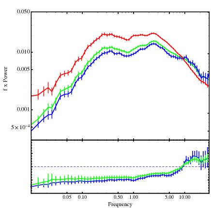
Figure 1: Upper panel: Power spectra in three energy bands from ObsID 10238-01-05-000: 3-5 keV (red), 10-20 keV (green) and 20-35 keV (blue). Lower panel: Ratio of power of the 10-20 keV band (green) and 20-35 keV band (blue) compared to the 3-5 keV band.

We fit the three power spectra using three Lorentzian functions (see Axelsson et al., 2005), and study the peak frequency in each band. The results are presented in Table 1. We find that the frequencies do not show any significant energy dependence.

	$\nu_{1}$ (Hz)	$\nu_{2}$ (Hz)	$\nu_{3}$ (Hz)
3–5 keV	0.29$\pm 0.01$	2.3$\pm 0.1$	–
10–20 keV	0.30$\pm 0.01$	2.3$\pm 0.1$	9.3$\pm 1.3$
20–35 keV	0.32$\pm 0.02$	2.3$\pm 0.1$	9.3$\pm 0.9$

Table 1: Peak frequencies of the three Lorentzian components in the three broad energy bands.

3.2 Time-averaged spectrum

We first attempt to fit the time-averaged spectrum, using both PCA and HEXTE data, with a single Comptonisation region, similar to the fits in Axelsson et al. (2013). This consists of thermal Comptonisation, parametrized using the model nthcomp in Xspec. We also include reflection (xilconv) and relativistic smearing (kdblur) of the Comptonised emission. For the smearing, the outer radius was frozen at 400 $r_{g}$ whereas the inner radius ($r_{\rm in}$) was left free. We characterise the interstellar absorption using use tbnew_gas, the updated version of tbabs (Wilms, Allen & McCray, 2000), with the assumption that all absorbing matter is neutral gas. The column density was frozen to $0.6\times 10^{22}$ cm^-2 (Nowak et al., 2011). We also include a normalisation constant between HEXTE and PCA, frozen at 0.9. Even if left free, the value does not change between models. We do not include a thermal component from the disc as the data only cover energies above 3 keV, which is too high to include much emission from a typical low/hard state temperature of 0.2 keV. We freeze the input seed photons of our Comptonisation components to this value (Ibragimov et al., 2005).

Our single-Comptonisation model is unable to provide a good fit to the data. This is not very surprising; as explained in Sect. 1 many studies have pointed to inhomogeneous Comptonisation being present in Cyg X-1. Following Ibragimov et al. (2005), we therefore add a second thermal Comptonisation component, again with seed photon temperature frozen to 0.2 keV. In terms of xspec components, the model becomes tbnew_gas$\times$(nthcomp+nthcomp+kdblur$\times$xilconv $\times$(nthcomp+nthcomp)). Note that xilconv is set to output only the reflected emission, and the parameters of its nthcomp arguments are tied to those of the direct emission. This now gives an excellent fit to the data. Details of the two models are given in Table 2.

Model	kTs (keV)	$\Gamma_{\rm s}$	norms	kTh (keV)	$\Gamma_{\rm h}$	normh	R	$\log\xi$	rin (rg)	$\chi^{2}$/dof
One Comp.	–	–	–	480${}^{+600}_{-160}$	1.68${}^{+0.002}_{-0.002}$	1.86${}^{+0.04}_{-0.04}$	0.37${}^{+0.03}_{-0.03}$	3.30${}^{+0.01}_{-0.01}$	45${}^{+unc}_{-20}$	216.9/100
Two Comp.	1.8${}^{+0.3}_{-0.3}$	2.01${}^{+0.23}_{-0.10}$	0.56${}^{+0.08}_{-0.21}$	116${}^{+20}_{-14}$	1.66${}^{+0.02}_{-0.01}$	1.94${}^{+0.09}_{-0.10}$	0.27${}^{+0.04}_{-0.04}$	2.98${}^{+0.08}_{-0.12}$	7${}^{+5}_{-2}$	52.2/97

Table 2: Parameter values for the best fit of the total spectrum to the spectral model using one or two thermal Comptonisation components. Subscripts s (soft) and h (hard) denote the two Comptonisation components, both of which have seed photons set to a 0.2 keV blackbody.

We stress that while the two-component fit found here is the best fit using this model, it is not necessarily comparable to those found in other studies, and it is not unique. Indeed, previous analyses have found that a wide range of combinations of two Comptonisation regions are able to provide good fits to the spectrum of Cyg X-1. Depending on the exact data set used, and using assumptions such as setting the same electron temperature for both regions, varying non-thermal electron fractions and different variations of the Comptonisation model, different conclusions are drawn about the properties of the Comptonisation (see, e.g., Ibragimov et al., 2005; Makishima et al., 2008; Nowak et al., 2011; Mahmoud & Done, 2018). This divergent set of results underscores the degeneracy inherent in spectral analysis, stressing the need to consider also information from temporal analysis.

3.3 Frequency resolved spectra

In the next step we extracted the frequency-resolved spectrum using the same techniques as in Axelsson et al. (2013). We extract the light curve for every available energy channel and construct its power density spectrum. These were fit with three Lorentzian components (L₁, L₂ and L₃). We found that allowing the peak frequencies to vary in every channel led to very large uncertainties, and therefore froze the peak frequencies to the average of those found in Table 1: 0.3, 2.3 and 9.3 Hz. This is justified since the frequencies did not change significantly between the energy bands (Table 1). With this approach we were able to constrain the components up to $\sim 30$  keV, above which the signal became too weak. In the first few channels, the highest frequency component is very weak, and its normalization is consistent with being zero. We integrate each Lorentzian in each energy channel to get an rms for that component at that energy, and multiply the time-averaged count rate by this value to extract frequency-resolved spectra corresponding to the noise components L₁ (red), L₂ (green) and L₃ (blue). These are presented along with the total spectrum in Fig. 2, where all the data are shown deconvolved against a power law of index -2 (i.e., flat in the $\nu F_{\nu}$ representation) to aid in the comparison.

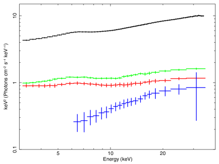
Figure 2: Upper panel: Extracted spectra from the three components in the power spectrum. In order of rising peak frequency: red (L₁), green (L₂) and blue (L₃). The total spectrum (black) is also shown for comparison. While L₁ and L₂ show spectra similar to the total, L₃ is dramatically differerent.

L₁ and L₂ (red and green points) show similar appearance to each other and to the total spectrum below 10 keV, including features around the 6.4 keV iron line, indicating reflection. However, both are much softer than the total spectrum above 10 keV. This is consistent with the study using AstroSat data presented by Misra et al. (2017), who found that the lower frequency component weakens more at higher energies. We see the same trend in our data (Fig. 2).

The most surprising behaviour is seen in the highest frequency component, L₃. As expected, it is not detected at low energies, likely being too weak. However, at higher energies the spectrum is radically different from the other two, more resembling a single power law than the total spectrum. It is also significantly harder and has no obvious reflection features (see also Revnivtsev et al., 1999).

The data from the variability components were then individually fit, using the spectral model from the total spectrum as template. The model was changed in steps until an acceptable fit was found. In the first step, the best-fit model for the total spectrum was merely scaled down, and tested against the data. Not surprisingly, this did not fit any of the variability components. L₁ and L₂ are softer than the total spectrum, whereas L₃ is too hard. In the second step, the relative normalisation between the two Comptonisation components was allowed to vary. This allowed us to find acceptable fits for L₁ and L₂, but not for L₃.

As L₃ is much harder than the total spectrum, it is clear that the slope of the hard Comptonisation component must change to provide a good fit. We therefore allowed this parameter to vary. However, we were still not able to find a good fit, unless we also let the seed photon temperature increase. Together, these two changes allowed us to find an acceptable fit to L₃ using a single Comptonisation component; no reflection is required. It seems then that L₃ provides us with a “pure” description of the hard Comptonisation!

In order to utilise this information, we now refit the total spectrum and L₃ together, tying the hard Comptonisation in the total spectrum to the variability spectrum, and allowing for different electron temperatures in the two Comptonisation components. The resulting fit quality is comparable to the one found before, but with the advantage that also L₃ can be fit. As before, allowing the relative normalisation to vary also allows good fits to L₁ and L₂. The results are presented in Table 3, and the resulting spectra with residuals shown in Fig. 3.

Comp	kTe,s	$\Gamma_{\rm s}$	norms	kTseed,h	kTe,h	$\Gamma_{\rm h}$	normh	R	$\log\xi$	rin	$\chi^{2}$/dof
	(keV)			(keV)	(keV)		$\times 10^{-2}$			(rg)
Total	2.1${}^{+0.2}_{-0.2}$	1.93${}^{+0.03}_{-0.03}$	2.82${}^{+0.11}_{-0.48}$	3.1†	145${}^{+50}_{-32}$	1.69${}^{+0.02}_{-0.03}$	1.8${}^{+0.4}_{-0.6}$	0.24${}^{+0.10}_{-0.05}$	3.00${}^{+0.24}_{-0.19}$	5.1${}^{+2.3}_{-1.5}$	61.6/171
L1	”	”	0.59${}^{+0.02}_{-0.02}$	”	”	”	0.22${}^{+0.01}_{-0.01}$	”	”	”
L2	”	”	0.67${}^{+0.01}_{-0.01}$	”	”	”	0.31${}^{+0.01}_{-0.01}$	”	”	”
L3	–	–	–	3.1${}^{+0.5}_{-0.3}$	”	”	0.20${}^{+0.03}_{-0.03}$	–	–	”

^†Value tied to that from L₃.

Table 3: Parameter values for the best fit to the spectral model tbnew_gas$\times$(nthcomp+nthcomp+kdblur $\times$xilconv $\times$(nthcomp+nthcomp)). The total spectrum and the three variability components were all fit together. Subscripts s (soft) and h (hard) denote the two Comptonisation components.

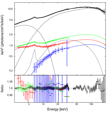
Figure 3: Fits of the total spectrum (black points) and frequency-resolved spectra (red, green and blue points). The gray lines show the Comptonisation (dashed) and reflection (dotted) components in the total spectrum. Solid lines show the total spectrum for both the total spectrum as well as each individual frequency-resolved spectrum. The bottom panel shows the ratio between the data and fitted model.

We note that the electron temperature of the soft Comptonisation component is almost comparable to the seed photon temperature of the hard Comptonisation. Attempting to tie these parameters gives an acceptable fit, yet slightly worse compared to those presented in Table 2. We therefore leave them separated.

The parameters in Table 3 also allow us to look at the ratio between normalisation parameters for the soft and hard Comptonisation components. This ratio (norm_s/norm_h) is 268 for L₁ and 216 for L₂, making it clear that the hard Comptonisation is relatively stronger in L₂ than in L₁. The same ratio is 112 in the total spectrum, indicating that the hard Comptonisation is less pronounced in the variability spectra compared to the total spectrum.

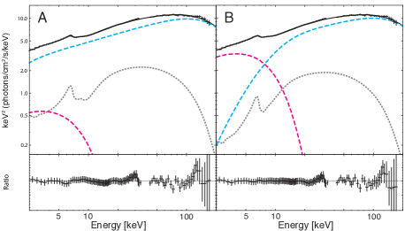
Figure 4: Comparison of spectral fits using different seed photon temperature for the hard Comptonisation component. A: Original model using kT_seed,h = 0.2 keV. $\chi^{2}$/dof = 52.2/97. B: Model using kT_seed,h = 3 keV, as indicated by the variability spectra. $\chi^{2}$/dof = 34.7/97. Upper panels show the data and model components: soft Comptonisation (magenta), hard Comptonisation (cyan) and reflection (gray). Lower panels show the ratio between data and model.

Finally, we compare the best-fit model found using the variability components with that presented in Table 2. The main difference between the models are that the seed photon temperature of the hard Comptonisation component is no longer set to 0.2 keV. Instead, we fix it at 3 keV, as indicated by the spectrum of L₃. Surprisingly, the resulting fit proves to be a significant improvement over the result in Table 2, with a $\chi^{2}$ of 34.7 compared to 52.2. Figure 4 shows a direct comparison between the two fits. Although both models give a good fit, using a higher seed photon temperature gives a significantly better fit statistic, and the PCA residuals improve. The model found by considering also the temporal information has thereby also led to a better global fit. This further strengthens the result that the two Comptonisation regions are spatially distinct, with the harder region seeing much more energetic seed photons.

The high seed photon temperature required by the data implies that the innermost region (where L₃ arises) is shielded from the disc photons. This in turn suggests that Comptonised emission arising in this region would not reach the disc, and thereby not be reprocessed. Unfortunately, the spectrum of L₃ does not allow us to test this prediction, as the uncertainties on the data are large (cf. the direct emission and reflection in Fig 4B). Allowing only the low-temperature Comptonisation component to be reflected in the total spectrum gives an acceptable but worse fit compared to the one in Table 3 ($\chi^{2}$/dof of 74.3/171 compared to 61.1/171). We therefore choose to keep the fit where both Comptonisation components are reflected. However, the worsening of the fit when considering the shielding effect of the softer component could be an indication that there are details in the data which our two-component model is unable to capture. We try to constrain these additional features in a model independent way below.

3.4 Isolating different radii

As described in Sect. 1, the broad-band variability likely arises due to propagating fluctuations in the accretion flow. In this picture, slower propagations arise in the outer regions of the flow, and as they propagate inwards, more rapid fluctuations are added. Variability at a given frequency is produced at a characteristic radius, so includes the spectrum produced at that radius, but then it propagates inwards so it is the sum of different spectral components at all radii interior to that where the characteristic frequency of the component is generated. This is shown schematically shown in Fig. 5, where the sketch is of a gradually stratified flow, with each region contributing a harder spectrum as the radius decreases, rather than the two component model used above.

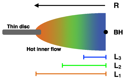
Figure 5: Cartoon picture showing the disc (grey) and regions of the inner accretion flow contributing to each variability component.

The cartoon image of Fig. 5 reveals a model-independent way to extract the spectra as a function of radius. By studying the difference between the variability spectra, we can attempt to isolate the spectrum which is characteristic of the radius at which each variability component is produced.

As described above, the highest frequencies are expected to be the “cleanest”. This is supported by our result that the spectrum of L₃ is well-fit by a single pure Comptonisation component. L₂ has a lower frequency, and it should therefore contain the same contributions as L₃, as well as emission from larger radii. To isolate the emission in the regions successively further out, we rescaled the L₃ spectrum to match that from L₂ in the highest energy bin (where the contribution is dominated by the innermost region), and then subtracted the L₃ spectrum. This is the maximum contribution from the hard innermost region, so this spectra is the softest that can be characteristic of the region where L₂ is produced. Similarly, we rescaled and subtracted the spectrum of L₂ from L₁. The results are shown in Fig. 6.

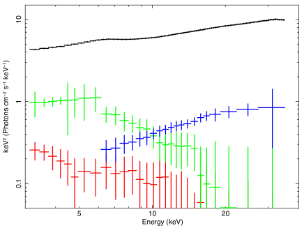
Figure 6: Spectra of each variability component after subtracting the contribution from higher frequencies (smaller radii). The colors are the same as in Fig. 2

While the data points have large uncertainties, some general features can still be distinguished. The spectrum characteristic of the largest radii (red) is the softest, and is subtly different to the shape of the soft Comptonisation in our two-component fits. The spectrum which can be associated with L₂ (green) is appreciably harder than that of L₁, while that of L₃ is well described by a single hard Comptonisation component with high electron temperature and seed photons around a few keV (as above).

These results suggest a more stratified region than in our two component model fits. Unfortunately, the data do not allow us to explore this further. However, it is clear that the technique has the potential to reveal even greater details of the stratified flow than shown in this study when combined with new data from NICER and/or AstroSat.

4 Discussion

It has been known for a long time that there are more than two components in the broad-band variability spectrum of Cyg X-1 (e.g., Nowak, 2000; Pottschmidt et al., 2003). However, the frequency range studied here (0.01-30 Hz) is dominated by two components, with a third entering only in the hardest observations (Axelsson et al., 2008). It is therefore interesting to see the presence of this third component in the higher energy bands, even when it is not evident in the lowest band.

Previous results have shown that the variability components change in response to spectral evolution of the source, becoming weaker and moving to higher frequencies as the hardness decreases (Pottschmidt et al., 2003; Axelsson et al., 2005, 2006; Grinberg et al., 2014). Our results indicate that there is also an energy dependence present. Because the frequencies do not change between the energy bands, it is likely that the third variability component appears due to increased relative strength as the energy increases - this is additionally supported by its hard spectrum. Having the strength of the component vary with energy also explains the result of Nowak (2000), who found that the best-fit combination of Lorentzian functions matching the power spectrum was dependent on energy.

In the spectral fits, we again confirm previous results that a single Comptonisation region is not sufficient to fit the spectrum of Cyg X-1. This is a general feature in many BHB systems (e.g., Ibragimov et al., 2005; Makishima et al., 2008; Yamada et al., 2013; Hjalmarsdotter et al., 2016). This result is further strengthened by the addition of the frequency-resolved data. While it is clear that both L₁ and L₂ show signs of Comptonisation, they are both softer than the total spectrum. There is thus no way that a single Comptonisation spectrum can explain both their spectra and the total. The point is driven home by L₃, which appears to match a clean Comptonisation spectrum, yet this spectrum is much too hard to explain the softer spectra. The only alternative is to allow multiple Comptonisation regions.

If there are indeed two (or more) separate Comptonisation components, as suggested by both the spectrum and the variability, they cannot be completely independent. If the two components would vary randomly with respect to each other, the rms is expected to be lower in the energy range where they contribute equally, as opposed to where one component dominates. There is no indication of such behaviour, either in the observations studied here or in previous works (e.g., Revnivtsev et al., 2001).

The smooth evolution of the rms instead supports the view of variability propagating through the flow, with each radius contributing most strongly at frequencies close to the local viscous timescale. Slower variations from the outer regions then modulate the faster variability, naturally coupling the variability at different timescales. This picture also couples higher frequencies to regions closer to the black hole, predicting that the energy spectrum of the variability components will get harder with increasing frequency. This matches the observations reported here, as well as many previous results.

While the slight differences between the first two variability components can be explained through sampling of different radii in a smoothly stratified flow, the third component is radically different, with seed photons as well as electrons being very energetic. As it is tied to the highest frequencies, it likely originates in the innermost part of the flow. The spectral shape then points to this region being shielded from the soft seed photons from the disc by the softer Comptonisation regions. Hence it should also have no reflection, as observed, although the uncertainties are large.

A further clue to the radial spectral stratification comes from subtracting the different frequency resolved spectra. Assuming the propagation framework is generally correct, these should mirror spectral components representative of the region where the variability component arises. While we are not able to directly fit any specific emission component to these spectra, the data by themselves indicate that L₂ arises in a higher-energy environment than L₁. Both components resemble Comptonised emission rather than a blackbody, pointing to an optically thin flow rather than the accretion disc itself, consistent with a truncated disc geometry.

We can now put all our results in the context of the accretion geometry. The similarity of the subtracted spectra to Comptonisation leads us to place the origin of the variability components in the hot inner flow. L₁ has both lowest frequency and the softest spectrum, and is thereby likely to arise furthest out in the flow. The spectrum of L₂ is slightly harder, placing it at smaller radii. However, both these variability spectra show clear signs of reflection (such as a noticeable iron line), indicating that they cannot arise too far away from the thin, optically thick disc. In contrast, L₃ has a very hard spectrum which shows no sign of reflection, placing its origin well inside the disc truncation radius and close to the innermost regions of the flow. The seed photon temperature of several keV also makes it likely that they come from Comptonisation in the outer parts of the hot flow, rather than directly from the disc. Combining emission from all these regions gives the total spectrum.

Even if we can paint a generally consistent picture, there are still questions which remain unanswered. For instance, a mechanism must be found to explain the frequencies of the variability components. If variability is created at all frequencies, why are these ones picked out? The most obvious answer is that the variability components are tied to certain radii in the flow, yet this does not match the fundamental assumption in propagation model, where fluctuations generated at one radii will propagate and thereby be present at all smaller radii. To prevent this, a mechanism must be invoked to allow one region to dominate, for example by assuming increased emissivity at certain radii (perhaps as a response to increased turbulence) or causing fluctuations to dampen as they propagate. However, our current results do not allow us to test any such hypotheses.

While the results reported here constitute an important step in breaking the spectral degeneracy, it is clear that there are many issues left to solve, both in the propagating fluctuations framework and to understand these data. For example, while Rapisarda et al. (2017b) were able to find good agreement between model and observations for power spectra, time lags and coherence as a function of energy in Cyg X-1 using propagating fluctuations, the same analysis showed discrepancies when applied to the BHB XTE J1550-564 (Rapisarda et al., 2017a). It is thus not surprising that also our results require the model to be refined in order to explain all observed features; indeed, such efforts are already underway (Mahmoud et al., in prep.). Equally important are more observational results, allowing us to look for systematic changes, for example as a function of spectral state. Such analysis is in progress, and will be reported in a future paper (Axelsson et al., in prep.).

5 Summary and Conclusions

We have analysed the broad-band variability of Cyg X-1 in the low/hard state using frequency-resolved spectroscopy. We find that the two main power spectral components, L₁ and L₂, have spectra which are too soft to match the total spectrum at higher energies. A third variability component appears at higher frequencies in the power spectrum, and this component has a drastically harder spectrum. This is mainly due to its seed photon energy being substantially higher than those seen by the flow at larger radii. These results can be interpreted in terms of propagating fluctuations through a Comptonisation clould which is radially stratified. The outer regions see the seed photons from the disc, and Compton cool on them, producing soft spectra. These regions also shield the inner parts of the flow from direct illumination by the disc as they are (moderately) optically thick. We model this directly using only two Comptonisation components, but subtraction of the spectral components indicates that there may be more gradual radial stratification of the outer region. This shows the potential of better data to directly deconvolve the radial properties of the hot inner flow, and hence determine whether this contains the imprint of the radius from which the compact jet is launched and powered.

References

- Arévalo & Uttley (2006) Arévalo P., Uttley P., 2006, MNRAS, 367, 801
- Axelsson et al. (2005) Axelsson M., Borgonovo L., Larsson S. 2005, A&A, 438, 999
- Axelsson et al. (2006) Axelsson, M., Borgonovo, L., & Larsson, S. 2006, A&A, 452, 975
- Axelsson et al. (2008) Axelsson M., Hjalmarsdotter L., Borgonovo L., Larsson S. 2008, A&A, 490, 253
- Axelsson et al. (2013) Axelsson M., Hjalmarsdotter L., Done C., 2013, MNRAS, 431, 1987
- Axelsson & Done (2016) Axelsson M., Done C. 2016, MNRAS, 458, 1778
- Basak et al. (2017) Basak, R., Zdziarski, A. A., Parker, M., & Islam, N. 2017, MNRAS, 472, 4220
- Di Salvo et al. (2001) Di Salvo, T., Done, C., Życki, P. T., Burderi, L., & Robba, N. R. 2001, ApJ, 547, 1024
- Done et al. (2007) Done, C., Gierliński, M., & Kubota, A. 2007, A&ARv, 15, 1
- Fabian et al. (2014) Fabian, A. C., Parker, M. L., Wilkins, D. R., et al. 2014, MNRAS, 439, 2307
- Gierliński et al. (1999) Gierliński, M., Zdziarski, A. A., Poutanen, J., et al. 1999, MNRAS, 309, 496
- Grinberg et al. (2014) Grinberg V., Pottschmidt K., Böck M., et al. 2014, A&A, 565, A1
- Hjalmarsdotter et al. (2016) Hjalmarsdotter L., Axelsson M., Done C. 2016, MNRAS, 456, 4354
- Ibragimov et al. (2005) Ibragimov A., Poutanen J., Gilfanov M., Zdziarski A. A., Shrader C. R. 2005, MNRAS, 362, 1435
- Jahoda et al. (1996) Jahoda K., Swank J. H., Giles A. B. et al. 1996, Proc. SPIE, 2808, 59
- Kotov et al. (2001) Kotov, O., Churazov, E., Gilfanov, M. 2001, MNRAS, 327, 799
- Lyubarskii (1997) Lyubarskii Y. E. 1997, MNRAS, 292, 679
- Mahmoud & Done (2018) Mahmoud, R. D., & Done, C. 2018, MNRAS, 473, 2084
- Makishima et al. (2008) Makishima K., Takahashi H., Yamada S., et al. 2008, PASJ, 60, 585
- Markoff et al. (2005) Markoff, S., Nowak, M. A., & Wilms, J. 2005, ApJ, 635, 1203
- Misra et al. (2017) Misra R., Yadav J.S., Verdhan Chauhan, J., et al. 2017, ApJ, 835, 195
- Nowak et al. (1999) Nowak M. A., Vaughan B. A., Wilms J., Dove J. B., Begelman M. C. 1999, ApJ, 510, 874
- Nowak (2000) Nowak M. A. 2000, MNRAS, 318, 361
- Nowak et al. (2011) Nowak, M. A., Hanke, M., Trowbridge, S. N., et al. 2011, ApJ, 728, 13
- Pottschmidt et al. (2003) Pottschmidt K., Wilms J., Nowak M. A., et al. 2003, A&A, 407, 1039
- Poutanen & Coppi (1998) Poutanen, J., & Coppi, P. S. 1998, Physica Scripta Volume T, 77, 57
- Rapisarda et al. (2017a) Rapisarda S., Ingram A., van der Klis, M. 2017a, MNRAS, 469, 2011
- Rapisarda et al. (2017b) Rapisarda S., Ingram A., van der Klis M. 2017b, MNRAS, 472, 3821
- Reig et al. (2002) Reig P., Papadakis I., Kylafis N. D. 2002, A&A, 383, 202
- Revnivtsev et al. (1999) Revnivtsev M., Gilfanov M., Churazov E. 1999, A&A, 347, L23
- Revnivtsev et al. (2000) Revnivtsev M., Gilfanov M., Churazov E. 2000, A&A, 363, 1013
- Revnivtsev et al. (2001) Revnivstev M., Gilfanov M., Churazov E. 2001, A&A, 380, 520
- Revnivtsev & Gilfanov (2006) Revnivtsev M. G., Gilfanov M. R. 2006, A&A, 453, 253
- Uttley & McHardy (2001) Uttley P., McHardy I. M. 2001, MNRAS, 323, L26
- Wilms, Allen & McCray (2000) Wilms J., Allen A., McCray R. 2000, ApJ, 542, 914
- Yamada et al. (2013) Yamada S., Makishima K., Done C., et al. 2013, PASJ, 65, 80
- Zdziarski et al. (2002) Zdziarski A. A., Poutanen J., Paciesas W. S., Wen, L. 2002, ApJ, 578, 357