A Virtual Element Method for the Transmission Eigenvalue Problem

Abstract

In this paper, we analyze a virtual element method (VEM) for solving a non-selfadjoint fourth-order eigenvalue problem derived from the transmission eigenvalue problem. We write a variational formulation and propose a $C^{1}$-conforming discretization by means of the VEM. We use the classical approximation theory for compact non-selfadjoint operators to obtain optimal order error estimates for the eigenfunctions and a double order for the eigenvalues. Finally, we present some numerical experiments illustrating the behavior of the virtual scheme on different families of meshes.

1 Introduction

In this work, we study a Virtual Element Method for an eigenvalue problem arising in scattering theory. The Virtual Element Method (VEM), introduced in [5, 7], is a generalization of the Finite Element Method which is characterized by the capability of dealing with very general polygonal/polyhedral meshes, and it also permits to easily implement highly regular discrete spaces. Indeed, by avoiding the explicit construction of the local basis functions, the VEM can easily handle general polygons/polyhedrons without complex integrations on the element (see [7] for details on the coding aspects of the method). The VEM has been developed and analyzed for many problems, see for instance [2, 3, 6, 9, 11, 13, 15, 17, 19, 20, 21, 29, 31, 36, 48, 52]. Regarding VEM for spectral problems, we mention [14, 37, 38, 44, 45, 46]. We note that there are other methods that can make use of arbitrarily shaped polygonal/polyhedral meshes, we cite as a minimal sample of them [8, 27, 35, 50].

Due to their important role in many application areas, there has been a growing interest in recent years towards developing numerical schemes for spectral problems (see [16]). In particular, we are going to analyze a virtual element approximation of the transmission eigenvalue problem. The motivation for considering this problem is that it plays an important role in inverse scattering theory [23, 33]. This is due to the fact that transmission eigenvalues can be determined from the far-field data of the scattered wave and used to obtain estimates for the material properties of the scattering object [22, 24].

In recent years various numerical methods have been proposed to solve this eigenvalue problem; see for example the following references [25, 26, 30, 34, 39, 42, 43, 49]. In particular, the transmission eigenvalue problem is often solved by reformulating it as a fourth-order eigenvalue problem. In [25], a $C^{1}$ finite element method using Argyris elements has been proposed, a complete analysis of the method including error estimates are proved using the theory for compact non-self-adjoint operators. However, the construction of conforming finite elements for $H^{2}(\Omega)$ is difficult in general, since they usually involve a large number of degrees of freedom (see [32]). More recently, in [39] a discontinuous Galerkin method has been proposed and analyzed to solve the fourth-order transmission eigenvalue problem; moreover, in [30] a $C^{0}$ linear finite element method has been introduced to solve the spectral problem.

The purpose of the present paper is to introduce and analyze a $C^{1}$-VEM for solving a fourth-order spectral problem derived from the transmission eigenvalue problem. We consider a variational formulation of the problem written in $H^{2}(\Omega)\times H^{1}(\Omega)$ as in [25, 39], where an auxiliary variable is introduced to transform the problem into a linear eigenvalue problem. Here, we exploit the capability of VEM to build highly regular discrete spaces (see [12, 19]) and propose a conforming $H^{2}(\Omega)\times H^{1}(\Omega)$ discrete formulation, which makes use of a very simple set of degrees of freedom, namely 4 degrees of freedom per vertex of the mesh. Then, we use the classical spectral theory for non-selfadjoint compact operators (see [4, 47]) to deal with the continuous and discrete solution operators, which appear as the solution of the continuous and discrete source problems, and whose spectra are related with the solutions of the transmission eigenvalue problem. Under rather mild assumptions on the polygonal meshes (made by possibly non-convex elements), we establish that the resulting VEM scheme provides a correct approximation of the spectrum and prove optimal-order error estimates for the eigenfunctions and a double order for the eigenvalues. Finally, we note that, differently from the FEM where building globally conforming $H^{2}(\Omega)$ approximation is complicated, here the virtual space can be built with a rather simple construction due to the flexibility of the VEM. In a summary, the advantages of the present virtual element discretization are the possibility to use general polygonal meshes and to build conforming $H^{2}(\Omega)$ approximations.

The remainder of this paper is structured as follows: In Section 2, we introduce the variational formulation of the transmission eigenvalue problem, define a solution operator and establish its spectral characterization. In Section 3, we introduce the virtual element discrete formulation, describe the spectrum of a discrete solution operator and establish some auxiliary results. In Section 4, we prove that the numerical scheme provides a correct spectral approximation and establish optimal order error estimates for the eigenvalues and eigenfunctions using the standard theory for compact and non-selfadjoint operators. Finally, we report some numerical tests that confirm the theoretical analysis developed in Section 5.

In this article, we will employ standard notations for Sobolev spaces, norms and seminorms. In addition, we will denote by $C$ a generic constant independent of the mesh parameter $h$, which may take different values in different occurrences.

2 The transmission eigenvalue problem

Let $\Omega\subset\mathbb{R}^{2}$ be a bounded domain with polygonal boundary $\partial\Omega$. We denote by $\nu$ the outward unit normal vector to $\partial\Omega$ and by $\partial_{\nu}$ the normal derivative. Let $n$ be a real value function in $L^{\infty}(\Omega)$ such that $n-1$ is strictly positive (or strictly negative) almost everywhere in $\Omega$. The transmission eigenvalue problem reads as follows:

Find the so-called transmission eigenvalue $k\in\mathbb{C}$ and a non-trivial pair of functions $(w_{1},w_{2})\in L^{2}(\Omega)\times L^{2}(\Omega)$, such that $(w_{1}-w_{2})\in H^{2}(\Omega)$ satisfying

$$\Delta w_{1}+k^{2}n(x)w_{1}=0 \quad\mbox{in }\Omega,$$ (2.1)

$$\Delta w_{2}+k^{2}w_{2}=0 \quad\mbox{in }\Omega,$$ (2.2)

$$w_{1}=w_{2} \quad\mbox{on }\partial\Omega,$$ (2.3)

$$\partial_{\nu}w_{1}=\partial_{\nu}w_{2} \quad\mbox{on }\partial\Omega.$$ (2.4)

Now, we rewrite problem above in the following equivalent form for $u:=(w_{1}-w_{2})\in H_{0}^{2}(\Omega)$ (see [25]):

Find $(k,u)\in\mathbb{C}\times H_{0}^{2}(\Omega)$ such that

$$(\Delta+k^{2}n)\frac{1}{n-1}(\Delta+k^{2})u=0 \quad\mbox{in }\Omega.$$ (2.5)

The variational formulation of problem (2.5) can be stated as: Find $(k,u)\in\mathbb{C}\times H_{0}^{2}(\Omega)$, $u\neq 0$ such that

$$\int_{\Omega}\frac{1}{n-1}(\Delta u+k^{2}u)(\Delta\overline{v}+k^{2}n\overline{v})=0 \quad\forall v\in H_{0}^{2}(\Omega),$$ (2.6)

where $\overline{v}$ denotes the complex conjugate of $v$. Now, expanding the previous expression we obtain the following quadratic eigenvalue problem:

$$\int_{\Omega}\frac{1}{n-1}\Delta u\Delta\overline{v}+\tau\int_{\Omega}\frac{1}{n-1}u\Delta\overline{v}+\tau\int_{\Omega}\frac{1}{n-1}\Delta u\overline{nv}+\tau^{2}\int_{\Omega}\frac{1}{n-1}u\overline{nv}=0\quad\forall v\in H_{0}^{2}(\Omega),$$ (2.7)

where $\tau:=k^{2}$. It is easy to show that $k=0$ is not an eigenvalue of the problem (see [25]). Moreover, for the sake of simplicity, we will assume that the index of refraction function $n(x)$ as a real constant. Nevertheless, this assumption do not affect the generality of the forthcoming analysis.

For the theoretical analysis it is convenient to transform problem (2.7) into a linear eigenvalue problem. With this aim, let $\phi$ be the solution of the problem: Find $\phi\in H_{0}^{1}(\Omega)$ such that

$$\Delta\phi=\tau\frac{n}{n-1}u\quad \Omega,$$ in (2.8)

$$\phi=0\quad \partial\Omega.$$ on (2.9)

Therefore, by testing problem (2.8)-(2.9) with functions in $H_{0}^{1}(\Omega)$, we arrive at the following weak formulation of the problem:

Problem 1.

Find $(\lambda,u,\phi)\in\mathbb{C}\times H_{0}^{2}(\Omega)\times H_{0}^{1}(\Omega)$ with $(u,\phi)\neq 0$ such that

$$a((u,\phi),(v,\psi))=\lambda b((u,\phi),(v,\psi))\quad\forall(v,\psi)\in{H_{0}^{2}(\Omega)}\times H_{0}^{1}(\Omega),$$

where $\lambda=-\tau$ and the sesquilinear forms $a(\cdot,\cdot)$ and $b(\cdot,\cdot)$ are defined by

$$a((u,\phi),(v,\psi)):= \frac{1}{n-1}\int_{\Omega}D^{2}u:D^{2}\overline{v}+\int_{\Omega}\nabla\phi\cdot\nabla\overline{\psi},$$

$$b((u,\phi),(v,\psi)):= \frac{n}{n-1}\int_{\Omega}\Delta u\overline{v}+\frac{1}{n-1}\int_{\Omega}u\Delta\overline{v}-\int_{\Omega}\nabla\phi\cdot\nabla\overline{v}+\frac{n}{n-1}\int_{\Omega}u\overline{\psi},$$

for all $(u,\phi),(v,\psi)\in{H_{0}^{2}(\Omega)}\times H_{0}^{1}(\Omega)$. Moreover, $":"$ denotes the usual scalar product of $2\times 2$-matrices, $D^{2}u:=(\partial_{ij}u)_{1\leq i,j\leq 2}$ denotes the Hessian matrix of $u$.

We endow ${H_{0}^{2}(\Omega)}\times H_{0}^{1}(\Omega)$ with the corresponding product norm, which we will simply denote $\|(\cdot,\cdot)\|$.

Now, we note that the sesquilinear forms $a(\cdot,\cdot)$ and $b(\cdot,\cdot)$ are bounded forms. Moreover, we have that $a(\cdot,\cdot)$ is elliptic.

Lemma 2.1.

There exists a constant $\alpha_{0}>0$, depending on $\Omega$, such that

$$a((v,\psi),(v,\psi))\geq\alpha_{0}\left\|(v,\psi)\right\|^{2}\qquad\forall(v,\psi)\in{H_{0}^{2}(\Omega)}\times H_{0}^{1}(\Omega).$$

Proof.

The result follows immediately from the fact that $\{\|D^{2}v\|_{0,\Omega}^{2}+\|\nabla\psi\|_{0,\Omega}^{2}\}^{1/2}$ is a norm on ${H_{0}^{2}(\Omega)}\times H_{0}^{1}(\Omega)$, equivalent with the usual norm. ∎

We define the solution operator associated with Problem 1:

$$\begin{array}[]{clll}T:{H_{0}^{2}(\Omega)}\times H_{0}^{1}(\Omega)&\longrightarrow&{H_{0}^{2}(\Omega)}\times H_{0}^{1}(\Omega)\\ (f,g)&\longmapsto&T(f,g)=(\tilde{u},\tilde{\phi})\end{array}$$

as the unique solution (as a consequence of Lemma 2.1) of the corresponding source problem:

$$a((\tilde{u},\tilde{\phi}),(v,\psi))=b((f,g),(v,\psi))\quad\forall(v,\psi)\in{H_{0}^{2}(\Omega)}\times H_{0}^{1}(\Omega).$$ (2.10)

The linear operator $T$ is then well defined and bounded. Notice that $(\lambda,u,\phi)\in\mathbb{C}\times{H_{0}^{2}(\Omega)}\times H_{0}^{1}(\Omega)$ solves Problem 1 if and only if $(\mu,u,\phi)$, with $\mu:=\frac{1}{\lambda}$, is an eigenpair of $T$, i.e., $T(u,\phi)=\mu(u,\phi)$.

We observe that no spurious eigenvalues are introduced into the problem since if $\mu\neq 0$, $(0,\phi)$ is not an eigenfunction of the problem.

The following is an additional regularity result for the solution of the source problem (2.10) and consequently, for the generalized eigenfunctions of $T$.

Lemma 2.2.

There exist $s,t\in(1/2,1]$ and $C>0$ such that, for all $(f,g)\in{H_{0}^{2}(\Omega)}\times H_{0}^{1}(\Omega)$, the solution $(\tilde{u},\tilde{\phi})$ of problem (2.10) satisfies $\tilde{u}\in H^{2+s}(\Omega)$, $\tilde{\phi}\in H^{1+t}(\Omega)$, and

$$\|\tilde{u}\|_{2+s,\Omega}+\|\tilde{\phi}\|_{1+t,\Omega}\leq C\|(f,g)\|.$$

Proof.

The estimate for $\tilde{\phi}$ follows from the classical regularity result for the Laplace problem with its right-hand side in $L^{2}(\Omega)$. The estimate for $\tilde{u}$ follows from the classical regularity result for the biharmonic problem with its right-hand side in $H^{-1}(\Omega)$ (cf. [41]). ∎

Remark 2.1.

The constant $s$ in the lemma above is the Sobolev regularity for the biharmonic equation with the right-hand side in $H^{-1}(\Omega)$ and homogeneous Dirichlet boundary conditions. The constant $t$ is the Sobolev exponent for the Laplace problem with homogeneous Dirichlet boundary conditions. These constants only depend on the domain $\Omega$. If $\Omega$ is convex, then $s=t=1$. Otherwise, the lemma holds for all $s<s_{0}$ and $t<t_{0}$, where $s_{0},t_{0}\in(1/2,1]$ depend on the largest reentrant angle of $\Omega$.

Hence, because of the compact inclusions $H^{2+s}(\Omega)\hookrightarrow{H_{0}^{2}(\Omega)}$ and $H^{1+t}(\Omega)\hookrightarrow H_{0}^{1}(\Omega)$, we can conclude that $T$ is a compact operator. So, we obtain the following spectral characterization result.

Lemma 2.3.

The spectrum of $T$ satisfies $\mathop{\mathrm{sp}}\nolimits(T)=\{0\}\cup\{\mu_{k}\}_{k\in\mathbb{N}}$, where $\{\mu_{k}\}_{k\in\mathbb{N}}$ is a sequence of complex eigenvalues which converges to 0 and their corresponding eigenspaces lie in $H^{2+s}(\Omega)\times H^{1+t}(\Omega)$. In addition $\mu=0$ is an infinite multiplicity eigenvalue of $T$.

Proof.

The proof is obtained from the compactness of $T$ and Lemma 2.2. ∎

3 The virtual element discretization

In this section, we will write the $C^{1}$-VEM discretization of Problem 1. With this aim, we start with the mesh construction and the assumptions considered to introduce the discrete virtual element spaces.

Let $\left\{\mathcal{T}_{h}\right\}_{h}$ be a sequence of decompositions of $\Omega$ into polygons $K$ we will denote by $h_{K}$ the diameter of the element $K$ and $h$ the maximum of the diameters of all the elements of the mesh, i.e., $h:=\max_{K\in\mathcal{T}_{h}}h_{K}$. In what follows, we denote by $N_{K}$ the number of vertices of $K$, by $e$ a generic edge of $\left\{\mathcal{T}_{h}\right\}_{h}$ and for all $e\in\partial K$, we define a unit normal vector $\nu_{K}^{e}$ that points outside of $K$.

In addition, we will make the following assumptions as in [5, 14]: there exists a positive real number $C_{\mathcal{T}}$ such that, for every $h$ and every $K\in\mathcal{T}_{h}$,

• the ratio between the shortest edge and the diameter $h_{K}$ of $K$ is larger than $C_{\mathcal{T}}$;

• $K\in\mathcal{T}_{h}$ is star-shaped with respect to every point of a ball of radius $C_{\mathcal{T}}h_{K}$.

In order to introduce the method, we first define two preliminary discrete spaces as follows: For each polygon $K\in\mathcal{T}_{h}$ (meaning open simply connected set whose boundary is a non-intersecting line made of a finite number of straight line segments) we define the following finite dimensional spaces,

$$\widetilde{W}_{h}^{K}:=\left\{v_{h}\in{H^{2}(K)}:\Delta^{2}v_{h}\in\mathbb{P}_{2}(K),v_{h}|_{\partial K}\in C^{0}(\partial K),v_{h}|_{e}\in\mathbb{P}_{3}(e)\,\,\forall e\in\partial K,\right.$$

$$\left.\nabla v_{h}|_{\partial K}\in C^{0}(\partial K)^{2},\partial_{\nu}v_{h}|_{e}\in\mathbb{P}_{1}(e)\,\,\forall e\in\partial K\right\},$$

and

$$\widetilde{V}_{h}^{K}:=\{\psi_{h}\in H^{1}(K):\Delta\psi_{h}\in\mathbb{P}_{1}(K),\psi_{h}|_{\partial K}\in C^{0}(\partial K),\psi_{h}|_{e}\in\mathbb{P}_{1}(e)\ \forall e\in\partial K\},$$

where $\Delta^{2}$ represents the biharmonic operator and we have denoted by $\mathbb{P}_{k}(S)$ the space of polynomials of degree up to $k$ defined on the subset $S\subseteq\mathbb{R}^{2}$.

The following conditions hold:

• for any $v_{h}\in\widetilde{W}_{h}^{K}$ the trace on the boundary of $K$ is continuous and on each edge is a polynomial of degree 3;

• for any $v_{h}\in\widetilde{W}_{h}^{K}$ the gradient on the boundary is continuous and on each edge its normal (respectively tangential) component is a polynomial of degree 1 (respectively 2);

• for any $\psi_{h}\in\widetilde{V}_{h}^{K}$ the trace on the boundary of $K$ is continuous and on each edge is a polynomial of degree 1;

• $\mathbb{P}_{2}(K)\times\mathbb{P}_{1}(K)\subseteq\widetilde{W}_{h}^{K}\times\widetilde{V}_{h}^{K}$.

Next, with the aim to choose the degrees of freedom for both spaces, we will introduce three sets ${\bf D_{1}}$, ${\bf D_{2}}$ and ${\bf D_{3}}$. The first two sets (${\bf D_{1}},{\bf D_{2}}$) are provided by linear operators from $\widetilde{W}_{h}^{K}$ into $\mathbb{R}$ and the set ${\bf D_{3}}$ by linear operators from $\widetilde{V}_{h}^{K}$ into $\mathbb{R}$. For all $(v_{h},\psi_{h})\in\widetilde{W}_{h}^{K}\times\widetilde{V}_{h}^{K}$ they are defined as follows:

• ${\bf D_{1}}$ contains linear operators evaluating $v_{h}$ at the $N_{K}$ vertices of $K$,

• ${\bf D_{2}}$ contains linear operators evaluating $\nabla v_{h}$ at the $N_{K}$ vertices of $K$,

• ${\bf D_{3}}$ contains linear operators evaluating $\psi_{h}$ at the $N_{K}$ vertices of $K$.

Note that, as a consequence of definition of the discrete spaces, the output values of the three sets of operators ${\bf D_{1}}$, ${\bf D_{2}}$ and ${\bf D_{3}}$, are sufficient to uniquely determine $v_{h}$ and $\nabla v_{h}$ on the boundary of $K$, and $\psi_{h}$ on the boundary of $K$, respectively.

In order to construct the discrete scheme, we need some preliminary definitions. First, we split the forms $a(\cdot,\cdot)$ and $b(\cdot,\cdot)$, introduced in the previous section, as follows:

$$a((u,\phi),(v,\psi))=\sum_{K\in\mathcal{T}_{h}}a^{\Delta}_{K}(u,v)+a^{\nabla}_{K}(\phi,\psi),\qquad(u,\phi),(v,\phi)\in{H_{0}^{2}(\Omega)}\times H_{0}^{1}(\Omega),$$

$$b((u,\phi),(v,\psi))=\sum_{K\in\mathcal{T}_{h}}b_{K}((u,\phi),(v,\psi)),\qquad(u,\phi),(v,\phi)\in{H_{0}^{2}(\Omega)}\times H_{0}^{1}(\Omega),$$

with

$$a^{\Delta}_{K}(u,v):=\int_{K}D^{2}u:\,D^{2}\overline{v},\qquad u,v\in{H^{2}(K)},$$

$$a^{\nabla}_{K}(\phi,\psi):=\int_{K}\nabla\phi\cdot\nabla\overline{\psi},\qquad\phi,\psi\in H^{1}(K),$$

and for all $(u,\phi),(v,\phi)\in H^{2}(K)\times H^{1}(K)$,

$$b_{K}((u,\phi),(v,\psi)):=\frac{n}{n-1}\int_{K}\Delta u\overline{v}+\frac{1}{n-1}\int_{K}u\Delta\overline{v}-\int_{K}\nabla\phi\cdot\nabla\overline{v}+\frac{n}{n-1}\int_{K}u\overline{\psi}.$$

Now, we define the projector $\Pi_{2}^{\Delta}:\ H^{2}(K)\longrightarrow\mathbb{P}_{2}(K)\subseteq\widetilde{W}_{h}^{K}$ for each $v\in H^{2}(K)$ as the solution of

$$a^{\Delta}_{K}\big{(}\Pi_{2}^{\Delta}v,q\big{)} =a^{\Delta}_{K}(v,q)\qquad\forall q\in\mathbb{P}_{2}(K),$$ (3.1a)

$$((\Pi_{2}^{\Delta}v,q))_{K} =((v,q))_{K}\qquad\forall q\in\mathbb{P}_{1}(K),$$ (3.1b)

where $((\cdot,\cdot))_{K}$ is defined as follows:

$$((u,v))_{K}=\sum_{i=1}^{N_{K}}u(P_{i})v(P_{i})\qquad\forall u,v\in C^{0}(\partial K),$$

where $P_{i},1\leq i\leq N_{K}$, are the vertices of $K$. We note that the bilinear form $a^{\Delta}_{K}(\cdot,\cdot)$ has a non-trivial kernel, given by $\mathbb{P}_{1}(K)$. Hence, the role of condition (3.1b) is to select an element of the kernel of the operator. We observe that operator $\Pi_{2}^{\Delta}$ is well defined on $\widetilde{W}_{h}^{K}$ and, most important, for all $v\in\widetilde{W}_{h}^{K}$ the polynomial $\Pi_{2}^{\Delta}v$ can be computed using only the values of the operators ${\bf D_{1}}$ and ${\bf D_{2}}$ calculated on $v$. This follows easily with an integration by parts (see [3]).

In a similar way, we define the projector $\Pi_{1}^{\nabla}:\ H^{1}(K)\longrightarrow\mathbb{P}_{1}(K)\subseteq\widetilde{V}_{h}^{K}$ for each $\psi\in H^{1}(K)$ as the solution of

$$a^{\nabla}_{K}\big{(}\Pi^{\nabla}_{1}\psi,q\big{)} =a^{\nabla}_{K}(\psi,q)\qquad\forall q\in\mathbb{P}_{1}(K),$$ (3.2a)

$$(\Pi^{\nabla}_{1}\psi,1)_{\partial K} =(\psi,1)_{\partial K}.$$ (3.2b)

We observe that operator $\Pi^{\nabla}_{1}$ is well defined on $\widetilde{V}_{h}^{K}$ and, as before, for all $\psi\in\widetilde{V}_{h}^{K}$ the polynomial $\Pi^{\nabla}_{1}\psi$ can be computed using only the values of the operators ${\bf D_{3}}$ calculated on $\psi$, which follows by an integration by parts (see [1]).

Now, we introduce our local virtual spaces:

$$W^{K}_{h}:=\left\{v_{h}\in\widetilde{W}_{h}^{K}:\int_{K}(\Pi_{2}^{\Delta}v_{h})q=\int_{K}v_{h}q\qquad\forall q\in\mathbb{P}_{2}(K)\right\},$$

and

$$V^{K}_{h}:=\left\{\psi_{h}\in\widetilde{V}_{h}^{K}:\int_{K}(\Pi_{1}^{\nabla}\psi_{h})q=\int_{K}\psi_{h}q\qquad\forall q\in\mathbb{P}_{1}(K)\right\}.$$

It is clear that $W_{h}^{K}\times V_{h}^{K}\subseteq\widetilde{W}_{h}^{K}\times\widetilde{V}_{h}^{K}$. Thus, the linear operators $\Pi_{2}^{\Delta}$ and $\Pi_{1}^{\nabla}$ are well defined on $W_{h}^{K}$ and $V_{h}^{K}$, respectively.

In [3, Lemma 2.1] has been established that the sets of operators ${\bf D_{1}}$ and ${\bf D_{2}}$ constitutes a set of degrees of freedom for the space $W^{K}_{h}$. Moreover, the set of operators ${\bf D_{3}}$ constitutes a set of degrees of freedom for the space $V^{K}_{h}$ (see [1]).

We also have that $\mathbb{P}_{2}(K)\times\mathbb{P}_{1}(K)\subseteq W^{K}_{h}\times V^{K}_{h}$. This will guarantee the good approximation properties for the spaces.

To continue the construction of the discrete scheme, we will need to consider new projectors: First, we define the projector $\Pi_{2}^{\nabla}:\ H^{2}(K)\longrightarrow\mathbb{P}_{2}(K)$ for each $w\in H^{2}(K)$ as the solution of

$$a^{\nabla}_{K}\big{(}\Pi^{\nabla}_{2}w,q\big{)} =a^{\nabla}_{K}(w,q)\qquad\forall q\in\mathbb{P}_{2}(K),$$ (3.3a)

$$(\Pi^{\nabla}_{2}w,1)_{0,K} =(w,1)_{0,K}.$$ (3.3b)

Moreover, we consider the $L^{2}(\Omega)$ orthogonal projectors onto $\mathbb{P}_{l}(K)$, $l=1,2$ as follows: we define $\Pi_{l}^{0}:L^{2}(\Omega)\to\mathbb{P}_{l}(K)$ for each $p\in L^{2}(\Omega)$ by

$$\int_{K}(\Pi_{l}^{0}p)q=\int_{K}pq\qquad\forall q\in\mathbb{P}_{l}(K).$$ (3.4)

Now, due to the particular property appearing in definition of the space $W^{K}_{h}$, it can be seen that the right hand side in (3.4) is computable using $\Pi_{2}^{\Delta}v_{h}$, and thus $\Pi_{2}^{0}v_{h}$ depends only on the values of the degrees of freedom for $v_{h}$ and $\nabla v_{h}$. Actually, it is easy to check that on the space $W^{K}_{h}$ the projectors $\Pi_{2}^{0}v_{h}$ and $\Pi_{2}^{\Delta}v_{h}$ are the same operator. In fact:

$$\int_{K}(\Pi_{2}^{0}v_{h})q=\int_{K}v_{h}q=\int_{K}(\Pi_{2}^{\Delta}v_{h})q\qquad\forall q\in\mathbb{P}_{2}(K).$$ (3.5)

Repeating the arguments, it can be proved that $\Pi_{1}^{0}\phi_{h}$ and $\Pi_{1}^{\nabla}\phi_{h}$ are the same operator in $V^{K}_{h}$.

Now, for every decomposition $\mathcal{T}_{h}$ of $\Omega$ into simple polygons $K$, we introduce our the global virtual space denoted by $Z_{h}$ as follow:

$$Z_{h}:=W_{h}\times V_{h},$$

where

$$W_{h}:=\{v_{h}\in H_{0}^{2}(\Omega):v_{h}|_{K}\in W^{K}_{h}\}\quad\mbox{and}\quad V_{h}:=\{\psi_{h}\in H_{0}^{1}(\Omega):\psi_{h}|_{K}\in V^{K}_{h}\}.$$

A set of degrees of freedom for $Z_{h}$ is given by all pointwise values of $v_{h}$ and $\psi_{h}$ on all vertices of $\mathcal{T}_{h}$ together with all pointwise values of $\nabla v_{h}$ on all vertices of $\mathcal{T}_{h}$, excluding the vertices on $\partial\Omega$ (where the values vanishes). Thus, the dimension of $Z_{h}$ is four times the number of interior vertices of $\mathcal{T}_{h}$.

In what follows, we discuss the construction of the discrete version of the local forms. With this aim, we consider $s_{K}^{\Delta}(\cdot,\cdot)$ and $s_{K}^{\nabla}(\cdot,\cdot)$ any symmetric positive definite forms satisfying:

$$c_{0}a_{K}^{\Delta}(v_{h},v_{h})\leq s_{K}^{\Delta}(v_{h},v_{h})\leq c_{1}a_{K}^{\Delta}(v_{h},v_{h}) \quad\forall v_{h}\in W_{h}^{K}\quad\mbox{with }\quad\Pi_{2}^{\Delta}v_{h}=0,$$ (3.6)

$$c_{2}a_{K}^{\nabla}(\psi_{h},\psi_{h})\leq s_{K}^{\nabla}(\psi_{h},\psi_{h})\leq c_{3}a_{K}^{\nabla}(\psi_{h},\psi_{h}) \quad\forall\psi_{h}\in V_{h}^{K}\quad\mbox{with }\quad\Pi_{1}^{\nabla}\psi_{h}=0.$$ (3.7)

We define the discrete sesquilinear forms $a_{h}(\cdot,\cdot):Z_{h}\times Z_{h}\to\mathbb{C}$ and $b_{h}(\cdot,\cdot):Z_{h}\times Z_{h}\to\mathbb{C}$ by

$$a_{h}((u_{h},\phi_{h}),(v_{h},\psi_{h})) :=\sum_{K\in\mathcal{T}_{h}}a_{h,K}^{\Delta}(u_{h},v_{h})+a_{h,K}^{\nabla}(\phi_{h},\psi_{h})\qquad\forall(u_{h},\phi_{h}),(v_{h},\psi_{h})\in Z_{h},$$

$$b_{h}((u_{h},\phi_{h}),(v_{h},\psi_{h})) :=\sum_{K\in\mathcal{T}_{h}}b_{h,K}((u_{h},\phi_{h}),(v_{h},\psi_{h}))\qquad\forall(u_{h},\phi_{h}),(v_{h},\psi_{h})\in Z_{h},$$

where $a_{h,K}^{\Delta}(\cdot,\cdot)$, $a_{h,K}^{\nabla}(\cdot,\cdot)$ and $b_{h,K}(\cdot,\cdot)$ are local forms on $W^{K}_{h}\times W^{K}_{h}$ and $V^{K}_{h}\times V^{K}_{h}$ defined by

$$a_{h,K}^{\Delta}(u_{h},v_{h}):=a_{K}^{\Delta}\big{(}\Pi_{2}^{\Delta}u_{h},\Pi_{2}^{\Delta}v_{h}\big{)}+s_{K}^{\Delta}\big{(}u_{h}-\Pi_{2}^{\Delta}u_{h},v_{h}-\Pi_{2}^{\Delta}v_{h}\big{)},\qquad\forall u_{h},v_{h}\in W^{K}_{h},$$

$$a_{h,K}^{\nabla}(\phi_{h},\psi_{h}):=a_{K}^{\nabla}\big{(}\Pi_{1}^{\nabla}\phi_{h},\Pi_{1}^{\nabla}\psi_{h}\big{)}+s_{K}^{\nabla}\big{(}\phi_{h}-\Pi_{1}^{\nabla}\phi_{h},\psi_{h}-\Pi_{1}^{\nabla}\psi_{h}\big{)},\qquad\forall\phi_{h},\psi_{h}\in V_{h}^{K},$$

$$b_{h,K}((u_{h},\phi_{h}),(v_{h},\psi_{h})): =\frac{n}{n-1}\int_{K}\Pi_{2}^{0}(\Delta u_{h})\Pi_{2}^{0}v_{h}+\frac{1}{n-1}\int_{K}\Pi_{2}^{0}u_{h}\Pi_{2}^{0}(\Delta v_{h})-\int_{K}\nabla\Pi_{1}^{\nabla}\phi_{h}\cdot\nabla\Pi_{2}^{\nabla}v_{h}$$

$$+\frac{n}{n-1}\int_{K}\Pi_{2}^{0}u_{h}\Pi_{1}^{0}\psi_{h}\qquad\forall(u_{h},\phi_{h}),(v_{h},\psi_{h})\in W^{K}_{h}\times V^{K}_{h}.$$

The construction of the local sesquilinear forms guarantees the usual consistency and stability properties, as is stated in the proposition below. Since the proof follows standard arguments in the VEM literature, it is omitted.

Proposition 3.1.

The local forms $a_{h,K}^{\Delta}(\cdot,\cdot)$ and $a_{h,K}^{\nabla}(\cdot,\cdot)$ on each element $K$ satisfy

• Consistency: for all $h>0$ and for all $K\in\mathcal{T}_{h}$ we have that

  $$a_{h,K}^{\Delta}(v_{h},q)=a_{K}^{\Delta}(v_{h},q)\qquad\forall q\in\mathbb{P}_{2}(K),\quad\forall v_{h}\in W^{K}_{h},$$ (3.8)

  $$a_{h,K}^{\nabla}(\psi_{h},q)=a_{K}^{\nabla}(\psi_{h},q)\qquad\forall q\in\mathbb{P}_{1}(K),\quad\forall\psi_{h}\in V^{K}_{h}.$$ (3.9)

• Stability and boundedness: There exist positive constants $\alpha_{i},i=1,2,3,4,$ independent of $K$, such that:

  $$\alpha_{1}a_{K}^{\Delta}(v_{h},v_{h})\leq a_{h,K}^{\Delta}(v_{h},v_{h})\leq\alpha_{2}a_{K}^{\Delta}(v_{h},v_{h})\qquad\forall v_{h}\in W^{K}_{h},$$ (3.10)

  $$\alpha_{3}a_{K}^{\nabla}(\psi_{h},\psi_{h})\leq a_{h,K}^{\nabla}(\psi_{h},\psi_{h})\leq\alpha_{4}a_{K}^{\nabla}(\psi_{h},\psi_{h})\qquad\forall\psi_{h}\in V^{K}_{h}.$$ (3.11)

Now, we are in a position to write the virtual element discretization of Problem 1.

Problem 2.

Find $(\lambda_{h},u_{h},\psi_{h})\in\mathbb{C}\times Z_{h}$, $(u_{h},\phi_{h})\neq 0$ such that

$$a_{h}((u_{h},\phi_{h}),(v_{h},\psi_{h}))=\lambda_{h}b_{h}((u_{h},\phi_{h}),(v_{h},\psi_{h})).$$ (3.12)

It is clear that by virtue of (3.10) and (3.11) the sesquilinear form $a_{h}(\cdot,\cdot)$ is bounded. Moreover, we will show in the following lemma that $a_{h}(\cdot,\cdot)$ is also uniformly elliptic.

Lemma 3.1.

There exists a constant $\beta>0$, independent of $h$, such that

$$a_{h}((v_{h},\psi_{h}),(v_{h},\psi_{h}))\geq\beta\|(v_{h},\psi_{h})\|^{2}\qquad\forall(v_{h},\psi_{h})\in Z_{h}.$$

Proof.

The result is deduced from Lemma 2.1, (3.10) and (3.11). ∎

Now, we introduce the discrete solution operator $T_{h}$ which is given by

$$\begin{array}[]{cccll}T_{h}:&H_{0}^{2}(\Omega)\times H_{0}^{1}(\Omega)&\longrightarrow&H_{0}^{2}(\Omega)\times H_{0}^{1}(\Omega)&\\ &(f,g)&\longmapsto&T_{h}(f,g)=(\tilde{u}_{h},\tilde{\phi}_{h})&\end{array}$$

where $(\tilde{u}_{h},\tilde{\phi}_{h})\in Z_{h}$ is the unique solution of the corresponding discrete source problem

$$a_{h}((\tilde{u}_{h},\tilde{\phi}_{h}),(v_{h},\psi_{h}))=b_{h}((f,g),(v_{h},\psi_{h}))\qquad\forall(v_{h},\psi_{h})\in Z_{h}.$$ (3.13)

Because of Lemma 3.1, the linear operator $T_{h}$ is well defined and bounded uniformly with respect to $h$. Once more, as in the continuous case, $(\lambda_{h},u_{h},\phi_{h})\in\mathbb{C}\times Z_{h}$ solves Problem 2 if and only if $(\mu_{h},u_{h},\phi_{h})$, with $\mu_{h}:=\frac{1}{\lambda_{h}}$, is an eigenpair of $T_{h}$, i.e., $T_{h}(u_{h},\phi_{h})=\mu_{h}(u_{h},\phi_{h})$.

4 Spectral approximation and error estimates

To prove that $T_{h}$ provides a correct spectral approximation of $T$, we will resort to the classical theory for compact operators (see [4]). With this aim, we first recall the following approximation result which is derived by interpolation between Sobolev spaces (see for instance [40, Theorem I.1.4] from the analogous result for integer values of $s$). In its turn, the result for integer values is stated in [5, Proposition 4.2] and follows from the classical Scott-Dupont theory (see [18] and [3, Proposition 3.1]):

Proposition 4.1.

There exists a constant $C>0$, such that for every $v\in H^{\delta}(K)$ there exists $v_{\pi}\in\mathbb{P}_{k}(K)$, $k\geq 0$ such that

$$|v-v_{\pi}|_{\ell,K}\leq Ch_{K}^{\delta-\ell}|v|_{\delta,K}\quad 0\leq\delta\leq k+1,\ell=0,\ldots,[\delta],$$

with $[\delta]$ denoting largest integer equal or smaller than $\delta\in{\mathbb{R}}$.

For the analysis we will introduce some broken seminorms:

$$|\psi|_{1,h}^{2}:=\sum_{K\in\mathcal{T}_{h}}|\psi|_{1,K}^{2}\qquad\mbox{and }\quad|v|_{2,h}^{2}:=\sum_{K\in\mathcal{T}_{h}}|v|_{2,K}^{2},$$

which are well defined for every $(\psi,v)\in[L^{2}(\Omega)]^{2}$ such that $(\psi,v)|_{K}\in H^{1}(K)\times H^{2}(K)$ for all polygon $K\in\mathcal{T}_{h}$.

In what follows, we derive several auxiliary results which will be used in the following to prove convergence and error estimates for the spectral approximation.

Proposition 4.2.

Assume A1–A2 are satisfied, let $\psi\in H^{1+t}(\Omega)$ with $t\in(0,1]$. Then, there exist $\psi_{I}\in V_{h}$ and $C>0$ such that

$$\|\psi-\psi_{I}\|_{1,\Omega}\leq Ch^{t}|\psi|_{1+t,\Omega}.$$

Proof.

This result has been proved in [28, Theorem 11] (see also [45, Proposition 4.2]). ∎

Proposition 4.3.

Assume A1–A2 are satisfied, let $v\in{H^{2+s}(\Omega)}$ with $s\in(0,1]$. Then, there exist $v_{I}\in W_{h}$ and $C>0$ such that

$$\|v-v_{I}\|_{2,\Omega}\leq Ch^{s}|v|_{2+s,\Omega}.$$

Proof.

This result has been establish in [3, Proposition 3.1]. ∎

Now, we establish a result which will be useful to prove the convergence of the operator $T_{h}$ to $T$ as $h$ goes to zero.

Lemma 4.1.

There exists $C>0$ independent of $h$ such that for all $(f,g)\in H_{0}^{2}(\Omega)\times H_{0}^{1}(\Omega)$, if $(\tilde{u},\tilde{\phi}):=T(f,g)$ and $(\tilde{u}_{h},\tilde{\phi}_{h}):=T_{h}(f,g)$, then

$$\left\|\left(T-T_{h}\right)(f,g)\right\|\leq Ch\|(f,g)\|+|\tilde{u}-\tilde{u}_{I}|_{2,\Omega}+|\tilde{u}-\tilde{u}_{\pi}|_{2,h}+|\tilde{\phi}-\tilde{\phi}_{I}|_{1,\Omega}+|\tilde{\phi}-\tilde{\phi}_{\pi}|_{1,h},$$

for all $(\tilde{u}_{I},\tilde{\phi}_{I})\in Z_{h}$ and for all $(\tilde{u}_{\pi},\tilde{\phi}_{\pi})\in[L^{2}(\Omega)]^{2}$ such that $(\tilde{u}_{\pi},\tilde{\phi}_{\pi})|_{K}\in\mathbb{P}_{2}(K)\times\mathbb{P}_{1}(K)$.

Proof.

Let $(f,g)\in H_{0}^{2}(\Omega)\times H_{0}^{1}(\Omega)$, for any $(\tilde{u}_{I},\tilde{\phi}_{I})\in W_{h}\times V_{h}$, we have,

$$\|(T-T_{h})(f,g)\|\leq\|(\tilde{u},\tilde{\phi})-(\tilde{u}_{I},\tilde{\phi}_{I})\|+\|(\tilde{u}_{I},\tilde{\phi}_{I})-(\tilde{u}_{h},\tilde{\phi}_{h})\|.$$ (4.1)

Now, we define $(v_{h},\psi_{h})=(\tilde{u}_{h}-\tilde{u}_{I},\tilde{\phi}_{h}-\tilde{\phi}_{I})\in Z_{h}$, then from the ellipticity of $a_{h}(\cdot,\cdot)$ and the definition of $T$ and $T_{h}$, we have

$$\beta\|(v_{h},\psi_{h})\|^{2}\leq a_{h}((v_{h},\psi_{h}),(v_{h},\psi_{h}))=a_{h}((\tilde{u}_{h},\tilde{\phi}_{h}),(v_{h},\psi_{h}))-a_{h}((\tilde{u}_{I},\tilde{\phi}_{I}),(v_{h},\psi_{h}))$$

$$=b_{h}((f,g),(v_{h},\psi_{h}))-\sum_{K\in\mathcal{T}_{h}}\Big{\{}a_{h,K}^{\Delta}(\tilde{u}_{I},v_{h})+a_{h,K}^{\nabla}(\tilde{\phi}_{I},\psi_{h})\Big{\}}$$

$$=b_{h}((f,g),(v_{h},\psi_{h}))-\sum_{K\in\mathcal{T}_{h}}\Big{\{}a_{h,K}^{\Delta}(\tilde{u}_{I}-\tilde{u}_{\pi},v_{h})+a_{h,K}^{\Delta}(\tilde{u}_{\pi},v_{h})+a_{h,K}^{\nabla}(\tilde{\phi}_{I}-\tilde{\phi}_{\pi},\psi_{h})+a_{h,K}^{\nabla}(\tilde{\phi}_{\pi},\psi_{h})\Big{\}}$$

$$=b_{h}((f,g),(v_{h},\psi_{h}))-\sum_{K\in\mathcal{T}_{h}}\Big{\{}a_{h,K}^{\Delta}(\tilde{u}_{I}-\tilde{u}_{\pi},v_{h})+a_{K}^{\Delta}(\tilde{u}_{\pi}-\tilde{u},v_{h})+a_{K}^{\Delta}(\tilde{u},v_{h})$$

$$\hskip 142.26378pt+a_{h,K}^{\nabla}(\tilde{\phi}_{I}-\tilde{\phi}_{\pi},\psi_{h})+a_{K}^{\nabla}(\tilde{\phi}_{\pi}-\tilde{\phi},\psi_{h})+a_{K}^{\nabla}(\tilde{\phi},\psi_{h})\Big{\}}$$

$$=\underbrace{\sum_{K\in\mathcal{T}_{h}}\Big{\{}b_{h,K}((f,g),(v_{h},\psi_{h}))-b_{K}((f,g),(v_{h},\psi_{h}))\Big{\}}}_{E_{1}}-\underbrace{\sum_{K\in\mathcal{T}_{h}}\Big{\{}a_{h,K}^{\Delta}(\tilde{u}_{I}-\tilde{u}_{\pi},v_{h})+a_{K}^{\Delta}(\tilde{u}_{\pi}-\tilde{u},v_{h})\Big{\}}}_{E_{2}}$$

$$-\underbrace{\sum_{K\in\mathcal{T}_{h}}\Big{\{}a_{h,K}^{\nabla}(\tilde{\phi}_{I}-\tilde{\phi}_{\pi},\psi_{h})+a_{K}^{\nabla}(\tilde{\phi}_{\pi}-\tilde{\phi},\psi_{h})\Big{\}}}_{E_{3}},$$ (4.2)

where we have used the consistency properties (3.8)-(3.9). We now bound each term $E_{i}|_{K}$, $i=1,2,3$.

First, the term $E_{1}|_{K}$ can be written as follows:

$$b_{h,K}((f,g),(v_{h},\psi_{h}))-b_{K}((f,g),(v_{h},\psi_{h}))$$

$$=\frac{n}{n-1}\Big{\{}\underbrace{\int_{K}\Pi_{2}^{0}(\Delta f)\Pi_{2}^{0}v_{h}-\int_{K}\Delta f\overline{v_{h}}}_{E_{11}}\Big{\}}+\frac{1}{n-1}\Big{\{}\underbrace{\int_{K}\Pi_{2}^{0}f\Pi_{2}^{0}(\Delta v_{h})-\int_{K}f\Delta\overline{v_{h}}}_{E_{12}}\Big{\}}$$

$$-\Big{\{}\underbrace{\int_{K}\nabla\Pi_{1}^{\nabla}g\cdot\nabla\Pi_{2}^{\nabla}v_{h}-\int_{K}\nabla g\cdot\nabla\overline{v_{h}}}_{E_{13}}\Big{\}}+\frac{n}{n-1}\Big{\{}\underbrace{\int_{K}(\Pi_{2}^{0}f)(\Pi_{1}^{0}\psi_{h})-\int_{K}f\overline{\psi_{h}}}_{E_{14}}\Big{\}}.$$ (4.3)

Now, we will bound each term $E_{1i}|_{K}\ i=1,2,3,4$. The term $E_{11}$ can be bounded as follows: Using the definition of $\Pi_{2}^{0}$ and Proposition 4.1, we have

$$E_{11} =\int_{K}\Delta f(\overline{v_{h}}-\Pi_{2}^{0}v_{h})\leq|f|_{2,K}||v_{h}-\Pi_{2}^{0}v_{h}||_{0,K}$$

$$=|f|_{2,K}\inf_{q\in\mathbb{P}_{2}(K)}||v_{h}-q||_{0,K}\leq Ch_{K}^{2}|f|_{2,K}|v_{h}|_{2,K}.$$

For the term $E_{12}$, we repeat the same arguments to obtain:

$$E_{12}\leq Ch_{K}^{2}|f|_{2,K}|v_{h}|_{2,K}.$$

Now, we bound $E_{13}$. From the definition of $\Pi_{2}^{\nabla}$, we have

$$E_{13} =\int_{K}\nabla\Pi_{1}^{\nabla}g\cdot\nabla\overline{v_{h}}-\int_{K}\nabla g\cdot\nabla\overline{v_{h}}=\int_{K}\nabla(\Pi_{1}^{\nabla}g-g)\cdot\nabla\overline{v_{h}}$$

$$=\int_{K}\nabla(\Pi_{1}^{\nabla}g-g)\cdot\nabla(\overline{v_{h}}-\tilde{v}_{\pi})\leq|\Pi_{1}^{\nabla}g-g|_{1,K}|v_{h}-\tilde{v}_{\pi}|_{1,K}$$

$$\leq Ch_{K}|g|_{1,K}|v_{h}|_{2,K},$$

where we have used the definition and the stability of $\Pi_{1}^{\nabla}$ with $\tilde{v}_{\pi}\in\mathbb{P}_{1}(K)$ such that Proposition 4.1 holds true.

For the term $E_{14}$, we first use the definition of $\Pi_{2}^{0}$, the definition and the stability of $\Pi_{1}^{0}$ with respect to $\hat{f}_{\pi}\in\mathbb{P}_{1}(K)$ such that Proposition 4.1 holds true, thus, we have

$$E_{14} =\int_{K}f\Pi_{1}^{0}\psi_{h}-\int_{K}f\overline{\psi_{h}}=\int_{K}(f-\hat{f}_{\pi})(\Pi_{1}^{0}\psi_{h}-\overline{\psi_{h}})$$

$$\leq Ch_{K}^{2}|f|_{2,K}||\Pi_{1}^{0}\psi_{h}-\psi_{h}||_{0,K}\leq Ch_{K}^{2}|f|_{2,K}\|\psi_{h}\|_{0,K}.$$

Therefore, using the Cauchy-Schwarz inequality, we can deduce from (4.3) that

$$E_{1}\leq Ch||(f,g)||||(v_{h},\psi_{h})||.$$

Finally, from (4.2) we have

$$\beta||(v_{h},\psi_{h})||\leq C\Big{\{}h||(f,g)||+|u-u_{I}|_{2,\Omega}+|u-u_{\pi}|_{2,h}+|\phi-\phi_{I}|_{1,\Omega}+|\phi-\phi_{\pi}|_{1,h}\Big{\}}.$$

Therefore, the proof follows from (4.1) and the previous inequality. ∎

For the convergence and error analysis of the proposed virtual element scheme for the transmission eigenvalue problem, we first establish that $T_{h}\to T$ in norm as $h\to 0$. Then, we prove a similar convergence result for the adjoint operators $T^{*}$ and $T_{h}^{*}$ of $T$ and $T_{h}$, respectively.

Lemma 4.2.

There exist $C>0$ and $\tilde{s}\in(0,1]$, independent of $h$, such that

$$\|T-T_{h}\|\leq Ch^{\tilde{s}}.$$

Proof.

Let $(f,g)\in H_{0}^{2}(\Omega)\times H_{0}^{1}(\Omega)$ such that $||(f,g)||=1$, let $(\tilde{u},\tilde{\phi})$ and $(\tilde{u}_{h},\tilde{\phi}_{h})$ be the solution of problems (2.10) and (3.13), respectively, so that $(\tilde{u},\tilde{\phi}):=T(f,g)$ and $(\tilde{u}_{h},\tilde{\phi}_{h}):=T_{h}(f,g)$. From Lemma 4.1, we have

$$\left\|\left(T-T_{h}\right)(f,g)\right\| \leq Ch||(f,g)||+\|u-u_{I}\|_{2,\Omega}+|u-u_{\pi}|_{2,h}+\|\phi-\phi_{I}\|_{1,\Omega}+|\phi-\phi_{\pi}|_{1,h}$$

$$\leq C\left(h||(f,g)||+h^{s}||f||_{2,\Omega}+h^{t}||g||_{1,\Omega}\right)$$

$$\leq Ch^{\tilde{s}}||(f,g)||$$

where we have used the Propositions 4.1, 4.2 and 4.3, and Lemma 2.2, with $\tilde{s}:=\min\{s,t\}$. Thus, we conclude the proof. ∎

Let $T^{*}$ and $T_{h}^{*}:H_{0}^{2}(\Omega)\times H_{0}^{1}(\Omega)\to H_{0}^{2}(\Omega)\times H_{0}^{1}(\Omega)$ the adjoint operators of $T$ and $T_{h}$, respectively, defined by $T^{*}(f,g):=(\tilde{u}^{*},\tilde{\phi}^{*})$ and $T^{*}_{h}(f,g):=(\tilde{u}_{h}^{*},\tilde{\phi}_{h}^{*})$, where $(\tilde{u}^{*},\tilde{\phi}^{*})$ and $(\tilde{u}_{h}^{*},\tilde{\phi}_{h}^{*})$ are the unique solutions of the following problems:

$$a((v,\psi),(\tilde{u}^{*},\tilde{\phi}^{*}))=b((v,\psi),(f,g))\qquad\forall(v,\psi)\in H_{0}^{2}(\Omega)\times H_{0}^{1}(\Omega),$$ (4.4)

$$a_{h}((v_{h},\psi_{h}),(\tilde{u}_{h}^{*},\tilde{\phi}_{h}^{*}))=b_{h}((v_{h},\psi_{h}),(f,g))\qquad\forall(v_{h},\psi_{h})\in Z_{h}.$$ (4.5)

It is simple to prove that if $\mu$ is an eigenvalue of $T$ with multiplicity $m$, $\overline{\mu}$ is an eigenvalue of $T^{*}$ with the same multiplicity $m$.

Now, we will study the convergence in norm $T_{h}^{*}$ to $T^{*}$ as $h$ goes to zero. With this aim, first we establish an additional regularity result for the solution $(\tilde{u}^{*},\tilde{\phi}^{*})$ of problem (4.4).

Lemma 4.3.

There exist $s,t\in(1/2,1]$ and $C>0$ such that, for all $(f,g)\in{H_{0}^{2}(\Omega)}\times H_{0}^{1}(\Omega)$, the solution $(\tilde{u}^{*},\tilde{\phi}^{*})$ of problem (4.4) satisfies $\tilde{u}^{*}\in H^{2+s}(\Omega)$, $\tilde{\phi}^{*}\in H^{1+t}(\Omega)$, and

$$\|\tilde{u}^{*}\|_{2+s,\Omega}+\|\tilde{\phi}^{*}\|_{1+t,\Omega}\leq C\|(f,g)\|.$$

Proof.

The result follows repeating the same arguments used in the proof of Lemma 2.2. ∎

Remark 4.1.

We note that the constants $s$ and $t$ in Lemma 4.3 are the same as in Lemma 2.2.

Now, we are in a position to establish the following result.

Lemma 4.4.

There exist $C>0$ and $\tilde{s}\in(0,1]$, independent of $h$, such that

$$\|T^{*}-T_{h}^{*}\|\leq Ch^{\tilde{s}}.$$

Proof.

It is essentially identical to that of Lemma 4.1. ∎

Our final goal is to show convergence and obtain error estimates. With this aim, we will apply to our problem the theory from [4, 47] for non-selfadjoint compact operators.

We first recall the definition of spectral projectors. Let $\mu$ be a nonzero eigenvalue of $T$ with algebraic multiplicity $m$ and let $\Gamma$ be an open disk in the complex plane centered at $\mu$, such that $\mu$ is the only eigenvalue of $T$ lying in $\Gamma$ and $\partial\Gamma\cap\mathop{\mathrm{sp}}\nolimits(T)=\emptyset$. The spectral projectors $E$ and $E^{*}$ are defined as follows:

• The spectral projector of $T$ relative to $\mu$: $E:=(2\pi i)^{-1}\int_{\partial\Gamma}(z-T)^{-1}dz$;

• The spectral projector of $T^{*}$ relative to $\overline{\mu}$: $E^{*}:=(2\pi i)^{-1}\int_{\partial\Gamma}(z-T^{*})^{-1}dz.$

$E$ and $E^{*}$ are projections onto the space of generalized eigenvectors $R(E)$ and $R(E^{*})$, respectively. It is simple to prove that $R(E),R(E^{*})\in H^{2+s}(\Omega)\times H^{1+t}(\Omega)$.

Now, since $T_{h}\to T$ in norm, there exist $m$ eigenvalues (which lie in $\Gamma$) $\mu_{h}^{(1)},\ldots,\mu_{h}^{(m)}$ of $T_{h}$ (repeated according to their respective multiplicities) will converge to $\mu$ as $h$ goes to zero.

In a similar way, we introduce the following spectral projector $E_{h}:=(2\pi i)^{-1}\int_{\partial\Gamma}(z-T_{h})^{-1}dz$, which is a projector onto the invariant subspace $R(E_{h})$ of $T_{h}$ spanned by the generalized eigenvectors of $T_{h}$ corresponding to $\mu_{h}^{(1)},\ldots,\mu_{h}^{(m)}$.

We recall the definition of the gap $\widehat{\delta}$ between two closed subspaces $\mathcal{X}$ and $\mathcal{Y}$ of a Hilbert space $\mathcal{V}$:

$$\widehat{\delta}(\mathcal{X},\mathcal{Y}):=\max\left\{\delta(\mathcal{X},\mathcal{Y}),\delta(\mathcal{Y},\mathcal{X})\right\},$$

where

$$\delta(\mathcal{X},\mathcal{Y}):=\sup_{\mathbf{x}\in\mathcal{X}:\ \left\|x\right\|_{\mathcal{V}}=1}\delta(x,\mathcal{Y}),\quad\text{with }\delta(x,\mathcal{Y}):=\inf_{y\in\mathcal{Y}}\|x-y\|_{\mathcal{V}}.$$

Let $\mathcal{P}_{h}:=\mathcal{P}_{h}^{2}\times\mathcal{P}_{h}^{1}:H_{0}^{2}(\Omega)\times H_{0}^{1}(\Omega)\to Z_{h}\subseteq H_{0}^{2}(\Omega)\times H_{0}^{1}(\Omega)$ be the projector defined by

$$a(\mathcal{P}_{h}(u,\phi)-(u,\phi),(v_{h},\psi_{h}))=a^{\Delta}(\mathcal{P}_{h}^{2}u-u,v_{h})+a^{\nabla}(\mathcal{P}_{h}^{1}\phi-\phi,\psi_{h})=0\qquad\forall(v_{h},\psi_{h})\in Z_{h}.$$

We note that the form $a(\cdot,\cdot)$ is the inner product of $H_{0}^{2}(\Omega)\times H_{0}^{1}(\Omega)$. Therefore, we have

$$|(u,\phi)-\mathcal{P}(u,\phi)|_{H_{0}^{2}(\Omega)\times H_{0}^{1}(\Omega)}=\inf\limits_{(v_{h},\psi_{h})\in Z_{h}}|(u,\phi)-(v_{h},\psi_{h})|_{H_{0}^{2}(\Omega)\times H_{0}^{1}(\Omega)},$$ (4.6)

and

$$|\mathcal{P}(u,\phi)|_{H_{0}^{2}(\Omega)\times H_{0}^{1}(\Omega)}\leq|(u,\phi)|_{H_{0}^{2}(\Omega)\times H_{0}^{1}(\Omega)}\qquad\forall(u,\phi)\in H_{0}^{2}(\Omega)\times H_{0}^{1}(\Omega).$$ (4.7)

The following error estimates for the approximation of eigenvalues and eigenfunctions hold true.

Theorem 4.1.

There exists a strictly positive constant $C$ such that

$$\widehat{\delta}(R(E),R(E_{h})) \leq Ch^{\min\{s,t\}},$$ (4.8)

$$\left|\mu-\hat{\mu}_{h}\right| \leq Ch^{2\min\{s,t\}},$$ (4.9)

where $\hat{\mu}_{h}:=\frac{1}{m}\sum\limits_{k=1}^{m}\mu_{h}^{(k)}$ and with the constants $s$ and $t$ as in Lemmas 2.2 and 4.3 (see also Remark 2.1).

Proof.

As a consequence of Lemma 4.2, $T_{h}$ converges in norm to $T$ as $h$ goes to zero. Then, the proof of (4.8) follows as a direct consequence of Theorem 7.1 from [4] and the fact that, for $(f,g)\in R(E)$, $\|(f,g)\|_{H^{2+s}(\Omega)\times H^{1+t}(\Omega)}\leq\|(f,g)\|$, because of Lemma 2.2.

In what follows we will prove (4.9): assume that $T(u_{k},\phi_{k})=\mu(u_{k},\phi_{k})$, $k=1,\ldots,m$. Since $a(\cdot,\cdot)$ is an inner product in $H_{0}^{2}(\Omega)\times H_{0}^{1}(\Omega)$, we can choose a dual basis for $R(E^{*})$ denoted by $(u_{k}^{*},\phi_{k}^{*})\in H_{0}^{2}(\Omega)\times H_{0}^{1}(\Omega)$ satisfying

$$a((u_{k},\phi_{k}),(u_{l}^{*},\phi_{l}^{*}))=\delta_{k,l}.$$

Now, from [4, Theorem 7.2], we have that

$$|\mu-\hat{\mu}_{h}|\leq\frac{1}{m}\sum\limits_{k=1}^{m}|\langle(T-T_{h})(u_{k},\phi_{k}),(u_{k}^{*},\phi_{k}^{*})\rangle|+C||(T-T_{h})|_{R(E)}||||(T^{*}-T_{h}^{*})|_{R(E^{*})}||,$$

where $\langle\cdot,\cdot\rangle$ denotes the corresponding duality pairing.

Thus, in order to obtain (4.9), we need to bound the two terms on the right hand side above.

The second term can be easily bounded from Lemmas 4.2 and 4.4. In fact, we have

$$||(T-T_{h})|_{R(E)}||||(T^{*}-T_{h}^{*})|_{R(E^{*})}||\leq Ch^{2\min\{s,t\}}.$$ (4.10)

Next, we manipulate the first term as follows: adding and subtracting $(v_{h},\psi_{h})\in Z_{h}$ and using the definition of $T$ and $T_{h}$, we obtain,

$$\langle(T-T_{h})(u_{k},\phi_{k}),(u_{k}^{*},\phi_{k}^{*})\rangle=a((T-T_{h})(u_{k},\phi_{k}),(u_{k}^{*},\phi_{k}^{*}))$$

$$=a((T-T_{h})(u_{k},\phi_{k}),(u_{k}^{*},\phi_{k}^{*})-(v_{h},\psi_{h}))+a(T(u_{k},\phi_{k}),(v_{h},\psi_{h}))-a(T_{h}(u_{k},\phi_{k}),(v_{h},\psi_{h}))$$

$$=a((T-T_{h})(u_{k},\phi_{k}),(u_{k}^{*},\phi_{k}^{*})-(v_{h},\psi_{h}))+b((u_{k},\phi_{k}),(v_{h},\psi_{h}))-a(T_{h}(u_{k},\phi_{k}),(v_{h},\psi_{h}))$$

$$+a_{h}(T_{h}(u_{k},\phi_{k}),(v_{h},\psi_{h}))-b_{h}((u_{k},\phi_{k}),(v_{h},\psi_{h}))$$

$$=\Big{\{}a((T-T_{h})(u_{k},\phi_{k}),(u_{k}^{*},\phi_{k}^{*})-(v_{h},\psi_{h}))\Big{\}}+\Big{\{}b((u_{k},\phi_{k}),(v_{h},\psi_{h}))-b_{h}((u_{k},\phi_{k}),(v_{h},\psi_{h}))\Big{\}}$$

$$+\Big{\{}a_{h}(T_{h}(u_{k},\phi_{k}),(v_{h},\psi_{h}))-a(T_{h}(u_{k},\phi_{k}),(v_{h},\psi_{h}))\Big{\}}\qquad\forall(v_{h},\psi_{h})\in Z_{h}.$$ (4.11)

Now, we estimate each bracket in (4.11) separately. First, to bound the second bracket, we use the additional regularity of $(u_{k},\phi_{k})\in R(E)\subset H^{2+s}(\Omega)\times H^{1+t}(\Omega)$ and repeating the same steps used to derive (4.3) (in this case with $(u_{k},\phi_{k})$ instead of $(f,g)$), we have

$$b_{h,K}((u_{k},\phi_{k}),(v_{h},\psi_{h}))-b_{K}((u_{k},\phi_{k}),(v_{h},\psi_{h}))=E_{11}+E_{12}+E_{13}+E_{14}.$$

Now, we will bound each term $E_{1i}\ i=1,2,3,4$, as in the proof of Lemma 4.1, but in this case exploiting the additional regularity and the estimates in Lemmas 2.2 and 4.3 for $(u_{k},\phi_{k})\in R(E)$ and $(u_{k}^{*},\phi_{k}^{*})\in R(E^{*})$, respectively.

In particular, the terms $E_{11},E_{12}$ and $E_{14}$ can be bound exactly as in the proof of Lemma 4.1. However, for the term $E_{13}$, we proceed as follows:

$$E_{13} =\int_{K}\nabla\Pi_{1}^{\nabla}\phi_{k}\cdot\nabla\overline{v_{h}}-\int_{K}\nabla\phi_{k}\cdot\nabla\overline{v_{h}}=\int_{K}\nabla(\Pi_{1}^{\nabla}\phi_{k}-\phi_{k})\cdot\nabla\overline{v_{h}}$$

$$=\int_{K}\nabla(\Pi_{1}^{\nabla}\phi_{k}-\phi_{k})\cdot\nabla(\overline{v_{h}}-\tilde{v}_{h}^{\pi})\leq|\Pi_{1}^{\nabla}\phi_{k}-\phi_{k}|_{1,K}|v_{h}-\tilde{v}_{h}^{\pi}|_{1,K}$$

$$=\inf_{q_{h}\in\mathbb{P}_{1}(K)}|\phi_{k}-q_{h}|_{1,K}|v_{h}-\tilde{v}_{h}^{\pi}|_{1,K}\leq Ch_{K}^{1+t}|\phi_{k}|_{1+t,K}|v_{h}|_{2,K}$$

$$\leq Ch_{K}^{2\min\{s,t\}}|\phi_{k}|_{1+t,K}|v_{h}|_{2,K},$$

where we have used the definition of $\Pi_{1}^{\nabla}$ with $\tilde{v}_{h}^{\pi}\in\mathbb{P}_{1}(K)$ such that Proposition 4.1 holds true and the fact that $\phi_{k}\in H^{1+t}(\Omega)$ together with Proposition 4.1 again.

Therefore taking sum and using the additional regularity for $\phi_{k}$, together with Lemma 2.2, we obtain

$$\Big{\{}b((u_{k},\phi_{k}),(v_{h},\psi_{h}))-b_{h}((u_{k},\phi_{k}),(v_{h},\psi_{h}))\Big{\}}\leq Ch^{2\min\{s,t\}}||(u_{k},\phi_{k})||||(v_{h},\psi_{h})||\qquad\forall(v_{h},\psi_{h})\in Z_{h}.$$ (4.12)

Now, we estimate the third bracket in (4.11). Let $(w_{h},\xi_{h}):=T_{h}(u_{k},\phi_{k})$ and $\Pi_{h}^{K}$ be defined by $(\Pi_{h}^{K}(v,\psi))|_{K}:=(\Pi_{2}^{\Delta}v,\Pi_{1}^{\nabla}\psi)$ for all $K\in\mathcal{T}_{h}$ and for all $(v,\psi)\in H_{0}^{2}(\Omega)\times H_{0}^{1}(\Omega)$, where $\Pi_{2}^{\Delta}$ and $\Pi_{1}^{\nabla}$ have been defined in (3.1a)-(3.1b) and (3.2a)-(3.2b), respectively. Hence, we have

$$a_{h}((w_{h},\xi_{h}),(v_{h},\psi_{h}))-a((w_{h},\xi_{h}),(v_{h},\psi_{h}))=\sum_{K\in\mathcal{T}_{h}}\Big{\{}a_{h,K}((w_{h},\xi_{h}),(v_{h},\psi_{h}))-a_{K}((w_{h},\xi_{h}),(v_{h},\psi_{h}))\Big{\}}$$

$$=\sum_{K\in\mathcal{T}_{h}}\Big{\{}a_{h,K}((w_{h},\xi_{h})-(\Pi_{2}^{\Delta}w_{h},\Pi_{1}^{\nabla}\xi_{h}),(v_{h},\psi_{h}))+a_{K}((\Pi_{2}^{\Delta}w_{h},\Pi_{1}^{\nabla}\xi_{h})-(w_{h},\xi_{h}),(v_{h},\psi_{h}))\Big{\}}$$

$$=\sum_{K\in\mathcal{T}_{h}}\Big{\{}a_{h,K}((w_{h},\xi_{h})-(\Pi_{2}^{\Delta}w_{h},\Pi_{1}^{\nabla}\xi_{h}),(v_{h},\psi_{h})-(\Pi_{2}^{\Delta}v_{h},\Pi_{1}^{\nabla}\psi_{h}))$$

$$+a_{K}((\Pi_{2}^{\Delta}w_{h},\Pi_{1}^{\nabla}\xi_{h})-(w_{h},\xi_{h}),(v_{h},\psi_{h})-(\Pi_{2}^{\Delta}v_{h},\Pi_{1}^{\nabla}\psi_{h}))\Big{\}}$$

$$\leq C\sum_{K\in\mathcal{T}_{h}}\Big{\{}|(w_{h},\xi_{h})-(\Pi_{2}^{\Delta}w_{h},\Pi_{1}^{\nabla}\xi_{h})|_{H^{2}(K)\times H^{1}(K)}|(v_{h},\psi_{h})-(\Pi_{2}^{\Delta}v_{h},\Pi_{1}^{\nabla}\psi_{h})|_{H^{2}(K)\times H^{1}(K)}\Big{\}}$$

$$=C\sum_{K\in\mathcal{T}_{h}}\Big{\{}|T_{h}(u_{k},\phi_{k})-\Pi_{h}^{K}T_{h}(u_{k},\phi_{k})|_{H^{2}(K)\times H^{1}(K)}|(v_{h},\psi_{h})-\Pi_{h}^{K}(v_{h},\psi_{h})|_{H^{2}(K)\times H^{1}(K)}\Big{\}},$$ (4.13)

for all $(v_{h},\psi_{h})\in Z_{h}$, where we have used (3.8)-(3.9), Cauchy-Schwarz inequality and (3.10)-(3.11). Now, using the triangular inequality, we have that

$$|T_{h}(u_{k},\phi_{k})-\Pi_{h}^{K}T_{h}(u_{k},\phi_{k})|_{H^{2}(K)\times H^{1}(K)} \leq|T_{h}(u_{k},\phi_{k})-T(u_{k},\phi_{k})|_{H^{2}(K)\times H^{1}(K)}$$

$$+|\Pi_{h}^{K}T_{h}(u_{k},\phi_{k})-\Pi_{h}^{K}T(u_{k},\phi_{k})|_{H^{2}(K)\times H^{1}(K)}$$

$$+|\Pi_{h}^{K}T(u_{k},\phi_{k})-T(u_{k},\phi_{k})|_{H^{2}(K)\times H^{1}(K)}.$$

Thus, from (4.13), the above estimate, the stability of $\Pi_{h}^{K}$ and the additional regularity for $(u_{k},\phi_{k})$ together with Lemma 2.2, we have

$$a_{h}(T_{h}(u_{k},\phi_{k}),(v_{h},\psi_{h}))-a(T_{h}(u_{k},\phi_{k}),(v_{h},\psi_{h}))$$

$$\leq Ch^{\min\{s,t\}}||(u_{k},\phi_{k})||\sum_{K\in\mathcal{T}_{h}}|(v_{h},\psi_{h})-\Pi_{h}^{K}(v_{h},\psi_{h})|_{H^{2}(K)\times H^{1}(K)}\qquad\forall(v_{h},\psi_{h})\in Z_{h}.$$ (4.14)

Finally, we take $(v_{h},\psi_{h}):=\mathcal{P}(u_{k}^{*},\phi_{k}^{*})\in Z_{h}$ in (4.11). Thus, on the one hand, we bound the first bracket in (4.11) as follows,

$$a((T-T_{h})(u_{k},\phi_{k}),(u_{k}^{*},\phi_{k}^{*})-(v_{h},\psi_{h}))=a((T-T_{h})(u_{k},\phi_{k}),(u_{k}^{*},\phi_{k}^{*})-\mathcal{P}(u_{k}^{*},\phi_{k}^{*}))$$

$$\leq|(T-T_{h})(u_{k},\phi_{k})|_{H_{0}^{2}(\Omega)\times H_{0}^{1}(\Omega)}|(u_{k}^{*},\phi_{k}^{*})-\mathcal{P}(u_{k}^{*},\phi_{k}^{*})|_{H_{0}^{2}(\Omega)\times H_{0}^{1}(\Omega)}$$

$$=|(T-T_{h})(u_{k},\phi_{k})|_{H_{0}^{2}(\Omega)\times H_{0}^{1}(\Omega)}\inf\limits_{(r_{h},s_{h})\in Z_{h}}|(u_{k}^{*},\phi_{k}^{*})-(r_{h},s_{h})|_{H_{0}^{2}(\Omega)\times H_{0}^{1}(\Omega)}$$

$$\leq|(T-T_{h})(u_{k},\phi_{k})|_{H_{0}^{2}(\Omega)\times H_{0}^{1}(\Omega)}|(u_{k}^{*},\phi_{k}^{*})-((u_{k}^{*})_{I},(\phi_{k}^{*})_{I})|_{H_{0}^{2}(\Omega)\times H_{0}^{1}(\Omega)}$$

$$\leq Ch^{2{\min\{s,t\}}}||(u_{k}^{*},\phi_{k}^{*})||,$$

where we have used (4.6), Propositions 4.2 and 4.3, the additional regularity for $(u_{k}^{*},\phi_{k}^{*})$, Lemma 4.3 and Lemma 4.2.

On the other hand, from (4.14) we have that

$$|(v_{h},\psi_{h})-\Pi_{h}^{K}(v_{h},\psi_{h})| {}_{H^{2}(K)\times H^{1}(K)}=|\mathcal{P}(u_{k}^{*},\phi_{k}^{*})-\Pi_{h}^{K}\mathcal{P}(u_{k}^{*},\phi_{k}^{*})|_{H^{2}(K)\times H^{1}(K)}$$

$$\leq|\mathcal{P}(u_{k}^{*},\phi_{k}^{*})-(u_{k}^{*},\phi_{k}^{*})|_{H^{2}(K)\times H^{1}(K)}+|(u_{k}^{*},\phi_{k}^{*})-\Pi_{h}^{K}(u_{k}^{*},\phi_{k}^{*})|_{H^{2}(K)\times H^{1}(K)}$$

$$+|\Pi_{h}^{K}((u_{k}^{*},\phi_{k}^{*})-\mathcal{P}(u_{k}^{*},\phi_{k}^{*}))|_{H^{2}(K)\times H^{1}(K)}.$$

Then, using again (4.6), Propositions 4.2 and 4.3, the additional regularity for $(u_{k}^{*},\phi_{k}^{*})$, Lemma 4.3 and Lemma 4.2, we obtain from (4.14) that

$$a_{h}(T_{h}(u_{k},\phi_{k}),(v_{h},\psi_{h}))-a(T_{h}(u_{k},\phi_{k}),(v_{h},\psi_{h}))\leq Ch^{2{\min\{s,t\}}}||(u_{k},\phi_{k})||||(u_{k}^{*},\phi_{k}^{*})||.$$ (4.15)

Thus, from (4.11), (4.12) and (4.15), we obtain

$$|\langle(T-T_{h})(u_{k},\phi_{k}),(u_{k}^{*},\phi_{k}^{*})\rangle|\leq Ch^{2\min\{s,t\}}.$$ (4.16)

Therefore, the proof follows from estimates (4.10) and (4.16). ∎

Remark 4.2.

The error estimate for the eigenvalue $\mu$ of $T$ yield analogous estimate for the approximation of the eigenvalue $\lambda=1/\mu$ of Problem 1 by means of $\hat{\lambda}_{h}:=\frac{1}{m}\sum\limits_{k=1}^{m}\lambda_{h}^{(k)}$, where $\lambda_{h}^{(k)}=1/\mu_{h}^{(k)}$.

5 Numerical results

In this section we present a series of numerical experiments to solve the transmission eigenvalue problem with the Virtual Element scheme (3.12). However, to complete the choice of the VEM, we had to fix the forms $s_{K}^{\Delta}(\cdot,\cdot)$ and $s_{K}^{\nabla}(\cdot,\cdot)$ satisfying (3.6) and (3.7), respectively. For $s_{K}^{\Delta}(\cdot,\cdot)$, we consider the same definition as in [46]:

$$s_{K}^{\Delta}(u_{h},v_{h}):=\sigma_{K}\sum\limits_{i=1}^{N_{K}}[u_{h}(P_{i})v_{h}(P_{i})+h_{P_{i}}^{2}\nabla u_{h}(P_{i})\cdot\nabla v_{h}(P_{i})] \quad\forall u_{h},v_{h}\in W_{h}^{K},$$

where $P_{1},\ldots,P_{N_{K}}$ are the vertices of $K$, $h_{P_{i}}$ corresponds to the maximum diameter of the elements with $P_{i}$ as a vertex and $\sigma_{K}>0$ is a multiplicative factor to take into account the magnitude of the parameter and the $h$-scaling, for instance, in the numerical tests we have picked $\sigma_{K}>0$ as the mean value of the eigenvalues of the local matrix $a_{K}^{\Delta}\big{(}\Pi_{2}^{\Delta}u_{h},\Pi_{2}^{\Delta}v_{h}\big{)}$. This ensures that the stabilizing term scales as $a_{K}^{\Delta}(v_{h},v_{h})$. Now, a choice for $s_{K}^{\nabla}(\cdot,\cdot)$ is given by

$$s_{K}^{\nabla}(\phi_{h},\psi_{h}):=\sum\limits_{i=1}^{N_{K}}\phi_{h}(P_{i})\psi_{h}(P_{i}) \quad\forall\phi_{h},\psi_{h}\in V_{h}^{K},$$

which corresponds to the identity matrix of dimension $N_{K}$. A proof of (3.6) and (3.7) for the above choices could be derived following the arguments in [10]. Finally, we mention that the previous definitions are in accordance with the analysis presented in [45, 46] in order to avoid spectral pollution.

We have implemented in a MATLAB code the proposed VEM on arbitrary polygonal meshes, by following the ideas presented in [7]. Moreover, we compare our results with those existing in the literature, for example [25, 30, 34, 43]. We have considered three different domains, namely: square domain, a circular domain centered at the origin and an L-shaped domain.

5.1 Test 1: Square domain

In this test, we have taken $\Omega:=(0,1)^{2}$ and index of refraction $n=4$ and $n=16$. We have tested the method by using different families of meshes (see Figure 1):

• $\mathcal{T}_{h}^{1}$: triangular meshes;

• $\mathcal{T}_{h}^{2}$: rectangular meshes;

• $\mathcal{T}_{h}^{3}$: hexagonal meshes;

• $\mathcal{T}_{h}^{4}$: non-structured hexagonal meshes made of convex hexagons.

The refinement parameter $N$ used to label each mesh is the number of elements on each edge of the domain.

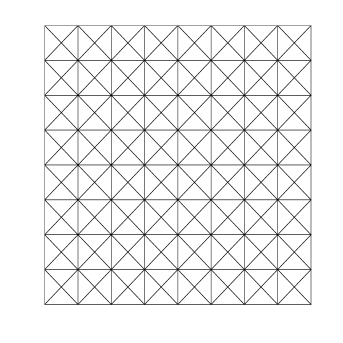
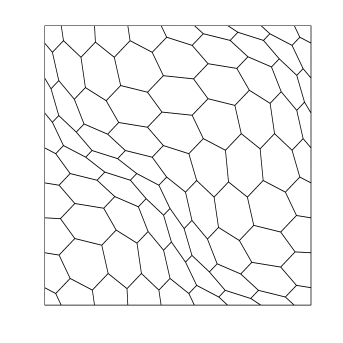
Figure 1: Sample meshes: $\mathcal{T}_{h}^{1}$ (top left), $\mathcal{T}_{h}^{2}$ (top right), $\mathcal{T}_{h}^{3}$ (bottom left) and $\mathcal{T}_{h}^{4}$ (bottom right), for $N=8$.

We report in Tables 1 and 2 the lowest transmission eigenvalues $k_{ih}$, $i=1,2,3,4$ computed by our method with two different families of meshes and $N=32,64,128,$ and with the index of refraction $n=16$ and $n=4$, respectively. The tables include computed orders of convergence, as well as more accurate values extrapolated by means of a least-squares fitting. Moreover, we compare the performance of the proposed method with those presented in [34, 43]. With this aim, we include in the last row of Tables 1 and 2 the results reported in that references, for the same problem.

Table 1: Test 1: Lowest transmission eigenvalues $k_{ih}$, $i=1,2,3,4$ computed on different meshes and with index of refraction $n=16$.

Meshes	$k_{ih}$	$k_{1h}$	$k_{2h}$	$k_{3h}$	$k_{4h}$
	$N=32$	1.8805	2.4467	2.4467	2.8691
	$N=64$	1.8798	2.4449	2.4449	2.8671
$\mathcal{T}_{h}^{1}$	$N=128$	1.8796	2.4444	2.4444	2.8666
	Order	2.01	2.00	2.00	2.01
	Extrapolated	1.8796	2.4442	2.4442	2.8664
	$N=32$	1.8764	2.4318	2.4318	2.8645
	$N=64$	1.8788	2.4410	2.4410	2.8658
$\mathcal{T}_{h}^{2}$	$N=128$	1.8794	2.4434	2.4434	2.8663
	Order	1.95	1.95	1.95	1.61
	Extrapolated	1.8796	2.4443	2.4443	2.8665
	[34, Argyris method]	1.8651	2.4255	2.4271	2.8178
	[34, Continuous method]	1.9094	2.5032	2.5032	2.9679
	[34, Mixed method]	1.8954	2.4644	2.4658	2.8918
	[43]	1.8796	2.4442	2.4442	2.8664

Table 2: Test 1: Lowest transmission eigenvalues $k_{ih}$, $i=1,2,3,4$ computed on different meshes and with index of refraction $n=4$.

Meshes	$k_{ih}$	$k_{1h}$	$k_{2h}$	$k_{3h}$	$k_{4h}$
	$N=32$	4.2835-1.1367	4.2835+1.1367	5.3373	5.4172
	$N=64$	4.2745-1.1446	4.2745+1.1446	5.4375	5.4599
$\mathcal{T}_{h}^{3}$	$N=128$	4.2724-1.1467	4.2724+1.1467	5.4661	5.4719
	Order	2.10& 1.89	2.10& 1.89	1.81	1.84
	Extrapolated	4.2717-1.1475	4.2717+1.1475	5.4775	5.4765
	$N=32$	4.2870-1.1341	4.2870+1.1341	5.3245	5.4178
	$N=64$	4.2753-1.1438	4.2753+1.1438	5.4329	5.4602
$\mathcal{T}_{h}^{4}$	$N=128$	4.2726-1.1465	4.2726+1.1465	5.4647	5.4719
	Order	2.12 &1.86	2.12&1.86	1.77	1.85
	Extrapolated	4.2718-1.1475	4.2718+1.1475	5.4779	5.4765
	[43]	4.2717-1.1474i	4.2717+1.1474i	5.4761	5.4761

It can be seen from Tables 1 and 2 that the eigenvalue approximation order of our method is quadratic (as predicted by the theory for convex domains) and that the results obtained by the two methods agree perfectly well.

5.2 Test 2: Circular domain

In this test, we have taken as domain the circle $\Omega:=\{(x,y)\in\mathbb{R}^{2}:x^{2}+y^{2}<1/2\}$. We have used polygonal meshes created with PolyMesher [51] (see Figure 2). The refinement parameter $N$ is the number of elements intersecting the boundary.

We report in Table 3 the five lowest transmission eigenvalues computed with the virtual element method analyzed in this paper. The table includes orders of convergence, as well as accurate values extrapolated by means of a least-squares fitting. Once again, the last rows show the values obtained by extrapolating those computed with different methods presented in [25, 30, 34].

Table 3: Test 2: Computed lowest transmission eigenvalues $k_{ih}$, $i=1,2,3,4,5$ with index of refraction $n=16$.

	$k_{1h}$	$k_{2h}$	$k_{3h}$	$k_{4h}$	$k_{5h}$
$N=32$	1.9835	2.6032	2.6037	3.2115	3.2117
$N=64$	1.9869	2.6105	2.6106	3.2225	3.2227
$N=128$	1.9877	2.6123	2.6123	3.2255	3.2256
Order	1.98	1.97	2.01	1.86	1.90
Extrapolated	1.9880	2.6129	2.6129	3.2267	3.2267
[25]	1.9881	-	-	-	-
[30]	1.9879	2.6124	2.6124	3.2255	3.2255
[34, Argyris method]	2.0076	2.6382	2.6396	3.2580	3.2598
[34, Continuous method]	2.0301	2.6937	2.6974	3.3744	3.3777
[34, Mixed method]	1.9912	2.6218	2.6234	3.2308	3.2397

Once more, a quadratic order of convergence can be clearly appreciated from Table 3.

We show in Figure 2 the eigenfunctions corresponding to the four lowest transmission eigenvalues.

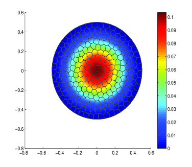
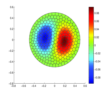
Figure 2: Test 2. Eigenfunctions $u_{1h}$ (top left), $u_{2h}$ (top right), $u_{3h}$ (bottom left) and $u_{4h}$ (bottom right).

5.3 Test 3: L-shaped domain

Finally, we have considered an L-shaped domain: $\Omega:=(-1/2,1/2)^{2}\backslash([0,1/2]\times[-1/2,0])$. We have used uniform triangular meshes as those shown in Figure 3. The meaning of the refinement parameter $N$ is the number of elements on each edge.

We report in Table 4 the four lowest transmission eigenvalues computed with the virtual scheme analyzed in this paper. The table includes orders of convergence, as well as accurate values extrapolated by means of a least-squares fitting. Once again, we compare the performance of the proposed virtual scheme with the one presented in [25] for the same problem, using triangular meshes.

Table 4: Test 3: Computed lowest transmission eigenvalues $k_{ih}$, $i=1,2,3,4$ with index of refraction $n=16$.

$k_{ih}$	$k_{1h}$	$k_{2h}$	$k_{3h}$	$k_{4h}$
$N=32$	2.9690	3.1480	3.4216	3.5744
$N=64$	2.9590	3.1417	3.4136	3.5683
$N=128$	2.9551	3.1400	3.4113	3.5667
Order	1.37	1.94	1.76	2.00
Extrapolated	2.9527	3.1395	3.4103	3.5662
[25]	2.9553	-	-	-

We notice that for the first transmission eigenvalue, the method converges with order close to $\min\{1.089,1.333\}$, which corresponds to the Sobolev regularity of the domain for the biharmonic equation and Laplace equation and with homogeneous Dirichlet boundary conditions, respectively (see [41]). Moreover, the method converges with larger orders for the rest of the transmission eigenvalues.

Finally, Figure 3 shows the eigenfunctions corresponding to the four lowest transmission eigenvalues with index of refraction $n=16$.

Figure 3: Test 3. Eigenfunctions $u_{1h}$ (top left), $u_{2h}$ (top right), $u_{3h}$ (bottom left) and $u_{4h}$ (bottom right).

References

• [1] B. Ahmad, A. Alsaedi, F. Brezzi, L. D. Marini and A. Russo, Equivalent projectors for virtual element methods, Comput. Math. Appl., 66, (2013), pp. 376–391.
• [2] P.F. Antonietti, L. Beirão da Veiga, D. Mora and M. Verani, A stream virtual element formulation of the Stokes problem on polygonal meshes, SIAM J. Numer. Anal., 52(1), (2014), pp. 386–404.
• [3] P.F. Antonietti, L. Beirão da Veiga, S. Scacchi and M. Verani, A $C^{1}$ virtual element method for the Cahn–Hilliard equation with polygonal meshes, SIAM J. Numer. Anal., 54(1), (2016), pp. 36–56.
• [4] I. Babuška and J. Osborn, Eigenvalue problems, in Handbook of Numerical Analysis, Vol. II, P.G. Ciarlet and J.L. Lions, eds., North-Holland, Amsterdam, 1991, pp. 641–787.
• [5] L. Beirão da Veiga, F. Brezzi, A. Cangiani, G. Manzini, L.D. Marini and A. Russo, Basic principles of virtual element methods, Math. Models Methods Appl. Sci., 23, (2013), pp. 199–214.
• [6] L. Beirão da Veiga, F. Brezzi and L.D. Marini, Virtual elements for linear elasticity problems, SIAM J. Numer. Anal., 51 (2013), pp. 794–812.
• [7] L. Beirão da Veiga, F. Brezzi, L.D. Marini and A. Russo, The hitchhiker’s guide to the virtual element method, Math. Models Methods Appl. Sci., 24, (2014), pp. 1541–1573.
• [8] L. Beirão da Veiga, K. Lipnikov and G. Manzini, The Mimetic Finite Difference Method for Elliptic Problems, Springer, MS&A, vol. 11, 2014.
• [9] L. Beirão da Veiga, C. Lovadina and D. Mora, A virtual element method for elastic and inelastic problems on polytope meshes, Comput. Methods Appl. Mech. Engrg., 295, (2015) pp. 327–346.
• [10] L. Beirão da Veiga, C. Lovadina and A. Russo, Stability analysis for the virtual element method, Math. Models Methods Appl. Sci., 27, (2017) pp. 2527–2594.
• [11] L. Beirão da Veiga, C. Lovadina and G. Vacca, Divergence free virtual elements for the Stokes problem on polygonal meshes, ESAIM Math. Model. Numer. Anal., 51(2), (2017) pp. 509–535.
• [12] L. Beirão da Veiga and G. Manzini, A virtual element method with arbitrary regularity, IMA J. Numer. Anal., 34, (2014), pp. 759–781.
• [13] L. Beirão da Veiga, D. Mora and G. Rivera, Virtual elements for a shear-deflection formulation of Reissner-Mindlin plates, Math. Comp., DOI: https://doi.org/10.1090/mcom/3331 (2017).
• [14] L. Beirão da Veiga, D. Mora, G. Rivera and R. Rodríguez, A virtual element method for the acoustic vibration problem, Numer. Math., 136(3), (2017), pp. 725–763.
• [15] M.F. Benedetto, S. Berrone, A. Borio, S. Pieraccini and S. Scialò, Order preserving SUPG stabilization for the virtual element formulation of advection–diffusion problems, Comput. Methods Appl. Mech. Engrg., 311, (2016), pp. 18–40.
• [16] D. Boffi, Finite element approximation of eigenvalue problems, Acta Numerica, 19 (2010), pp. 1–120.
• [17] S.C. Brenner, Q. Guan and L.-Y Sung, Some estimates for virtual element methods, Comput. Methods Appl. Math., 17(4), (2017), pp. 553–574.
• [18] S.C. Brenner and R.L. Scott, The Mathematical Theory of Finite Element Methods, Springer, New York, 2008.
• [19] F. Brezzi and L.D. Marini, Virtual elements for plate bending problems, Comput. Methods Appl. Mech. Engrg., 253, (2012), pp. 455–462.
• [20] E. Cáceres and G.N. Gatica, A mixed virtual element method for the pseudostress-velocity formulation of the Stokes problem, IMA J. Numer. Anal., 37(1), 2017, pp. 296–331.
• [21] E. Cáceres, G.N. Gatica and F. Sequeira, A mixed virtual element method for the Brinkman problem, Math. Models Methods Appl. Sci., 27(4), (2017) pp. 707–743.
• [22] F. Cakoni, M. Çayören and D. Colton, Transmission eigenvalues and the nondestructive testing of dielectrics, Inverse Problems, 24(6), (2008), 065016.
• [23] F. Cakoni, D. Colton, P. Monk and J. Sun, The inverse electromagnetic scattering problem for anisotropic media, Inverse Problems, 26(7), (2010), 074004.
• [24] F. Cakoni, D. Gintides and H. Haddar, The existence of an infinite discrete set of transmission eigenvalue, SIAM J. Math. Anal., 42, (2010), pp. 237–255.
• [25] F. Cakoni, P. Monk and J. Sun, Error analysis for the finite element approximation of transmission eigenvalues, Comput. Methods Appl. Math., 14(4), (2014), pp. 419–427.
• [26] J. Camaño, R. Rodríguez and P. Venegas, Convergence of a lowest-order finite element method for the transmission eigenvalue problem, CI2MA Preprint 2018–06, Universidad de Concepción.
• [27] A. Cangiani, E.H. Georgoulis and P. Houston, $hp$-version discontinuous Galerkin methods on polygonal and polyhedral meshes, Math. Models Methods Appl. Sci., 24(10), (2014), pp. 2009–2041.
• [28] A. Cangiani, E.H. Georgoulis, T. Pryer and O.J. Sutton, A posteriori error estimates for the virtual element method, Numer. Math., 137(4), (2017) pp. 857–893.
• [29] A. Cangiani, G. Manzini and O.J. Sutton, Conforming and nonconforming virtual element methods for elliptic problems, IMA J. Numer. Anal., 37(3), (2017), pp. 1317–1354.
• [30] H. Chen, H. Guo, Z. Zhang and Q. Zou, A $C^{0}$ linear finite element method for two fourth-order eigenvalue problems, IMA J. Numer. Anal., 37(4), (2017), pp. 2120–2138.
• [31] C. Chinosi and L.D. Marini, Virtual element method for fourth order problems: $L^{2}$-estimates, Comput. Math. Appl., 72(8), (2016), pp. 1959–1967.
• [32] P.G. Ciarlet, The Finite Element Method for Elliptic Problems, SIAM, Philadelphia, 2002.
• [33] D. Colton and R. Kress, Inverse Acoustic and Electromagnetic Scattering Theory, 3rd ed., Springer, New York, 2013.
• [34] D. Colton, P. Monk and J. Sun, Analytical and computational methods for transmission eigenvalues, Inverse Problems, 26(4), (2010), 045011.
• [35] D. Di Pietro and A. Ern, A hybrid high-order locking-free method for linear elasticity on general meshes, Comput. Methods Appl. Mech. Eng., 283, (2015), pp. 1–21.
• [36] M. Frittelli and I. Sgura, Virtual element method for the Laplace–Beltrami equation on surfaces, ESAIM Math. Model. Numer. Anal., DOI: https://doi.org/10.1051/m2an/2017040 (2017).
• [37] F. Gardini, G. Manzini and G. Vacca, The nonconforming virtual element method for eigenvalue problems, arXiv:1802.02942 [math.NA], (2018).
• [38] F. Gardini and G. Vacca, Virtual element method for second order elliptic eigenvalue problems, IMA J. Numer. Anal., DOI: https://doi.org/10.1093/imanum/drx063 (2017).
• [39] H. Geng, X. Ji, J. Sun and L. Xu, C0IP methods for the transmission eigenvalue problem, J. Sci. Comput., 68(1), (2016), pp. 326–338.
• [40] V. Girault and P.A. Raviart, Finite Element Methods for Navier-Stokes Equations, Springer-Verlag, Berlin, 1986.
• [41] P. Grisvard, Elliptic Problems in Non-Smooth Domains, Pitman, Boston, 1985.
• [42] J. Han, Y. Yang and H. Bi, Non-conforming finite element methodos for a transmission eigenvalue problem, Comput. Methods Appl. Mech. Engrg., 307, (2016), pp. 144–163.
• [43] J. Han, Y. Yang and H. Bi, A new multigrid finite element method for the transmission eigenvalue problems, Appl. Math. Comput., 292, (2017), pp. 96–106.
• [44] D. Mora and G. Rivera, A priori and a posteriori error estimates for a virtual element spectral analysis for the elasticity equations, arXiv:1712.06441 [math.NA], (2017).
• [45] D. Mora, G. Rivera and R. Rodríguez, A virtual element method for the Steklov eigenvalue problem, Math. Models Methods Appl. Sci., 25(8), (2015), pp. 1421–1445.
• [46] D. Mora, G. Rivera and I. Velásquez, A virtual element method for the vibration problem of Kirchhoff plates, ESAIM Math. Model. Numer. Anal., DOI: https://doi.org/10.1051/m2an/2017041 (2017).
• [47] J. Osborn, Spectral approximation for compact operators, Math. Comp., 29, (1975), pp 712–725.
• [48] I. Perugia, P. Pietra and A. Russo, A plane wave virtual element method for the Helmholtz problem, ESAIM Math. Model. Numer. Anal., 50(3), (2016), pp. 783–808.
• [49] J. Sun, Iterative methods for transmission eigenvalues, SIAM J. Numer. Anal., 49(5), (2011), pp. 1860–1874.
• [50] C. Talischi, G.H. Paulino, A. Pereira and I.F.M. Menezes, Polygonal finite elements for topology optimization: A unifying paradigm, Internat. J. Numer. Methods Engrg., 82(6), (2010), pp. 671–698.
• [51] C. Talischi, G.H. Paulino, A. Pereira and I.F.M. Menezes, PolyMesher: a general-purpose mesh generator for poygonal elements written in Matlab, Struct. Multidisc. Optim., 45, (2012), pp. 309–328.
• [52] G. Vacca, An $H^{1}$-conforming virtual element for Darcy and Brinkman equations, Math. Models Methods Appl. Sci., 28(1), (2018), pp. 159–194.