Moment-Based Quantile Sketches
for Efficient High Cardinality Aggregation Queries

Abstract.

Interactive analytics increasingly involves querying for quantiles over sub-populations of high cardinality datasets. Data processing engines such as Druid and Spark use mergeable summaries to estimate quantiles, but summary merge times can be a bottleneck during aggregation. We show how a compact and efficiently mergeable quantile sketch can support aggregation workloads. This data structure, which we refer to as the moments sketch, operates with a small memory footprint (200 bytes) and computationally efficient (50ns) merges by tracking only a set of summary statistics, notably the sample moments. We demonstrate how we can efficiently estimate quantiles using the method of moments and the maximum entropy principle, and show how the use of a cascade further improves query time for threshold predicates. Empirical evaluation shows that the moments sketch can achieve less than 1 percent quantile error with $15\times$ less overhead than comparable summaries, improving end query time in the MacroBase engine by up to $7\times$ and the Druid engine by up to $60\times$.

1. Introduction

Performing interactive multi-dimensional analytics over data from sensors, devices, and servers increasingly requires computing aggregate statistics for specific subpopulations and time windows (Rabkin et al., 2014; Feng et al., 2015; Agarwal et al., 2013). In applications such as A/B testing (Hill et al., 2017; Johari et al., 2017), exploratory data analysis (Bailis et al., 2017; Vartak et al., 2015), and operations monitoring (Beyer et al., 2016; Abraham et al., 2013), analysts perform aggregation queries to understand how specific user cohorts, device types, and feature flags are behaving. In particular, computing quantiles over these subpopulations is an essential part of debugging and real-time monitoring workflows (Dean and Barroso, 2013).

As an example of this quantile-driven analysis, our collaborators on a Microsoft application monitoring team collect billions of telemetry events daily from millions of heterogeneous mobile devices. Each device tracks multiple metrics including request latency and memory usage, and is associated with dimensional metadata such as application version and hardware model. Engineers issue quantile queries on a Druid-like (Yang et al., 2014) in-memory data store, aggregating across different dimensions to monitor their application (e.g., examine memory trends across device types) and debug regressions (e.g., examine tail latencies across versions). Querying for a single percentile in this deployment can require aggregating hundreds of thousands of dimension value combinations.

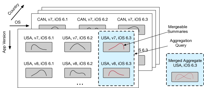
Figure 1. Given a data cube with pre-aggregated summaries, we can compute roll-ups by merging the relevant summaries. Efficiently mergeable summaries enable scalable aggregations.

When users wish to examine the quantiles of specific slices of a dataset, OLAP engines such as Druid and Spark support computing approximate quantiles using compressed representations (summaries) of the data values (Ray, 2013; Yang et al., 2014; Hunter et al., 2016; Zaharia et al., 2012). By pre-aggregating a summary for each combination of dimension values, Druid and similar engines can reduce query times and memory usage by operating over the relevant summaries directly, effectively constructing a data cube (Gray et al., 1997; Rabkin et al., 2014).

Given a time interval and a metric with $d$ associated dimensions, Druid maintains one pre-aggregated summary for each $d$-tuple of dimension values. These summaries are kept in RAM across a number of nodes, with each node scanning relevant summaries to process subsets of the data specified by a user query. Figure 1 illustrates how these mergeable (Agarwal et al., 2012) summaries can be aggregated to compute quantile roll-ups along different dimensions without scanning over the raw data.

More concretely, a Druid-like data cube in our Microsoft deployment with 6 dimension columns, each with $10$ distinct values, is stored as a set of up to $10^{6}$ summaries per time interval. On this cube, computing the 99-th percentile latency for a specific app version can require 100,000 merges, or even more for aggregation across complex time ranges. When there are a limited number of dimensions but enormous data volumes, it is cheaper to maintain these summaries than scan over billions of raw datapoints.

Many quantile summaries support the merge operation (Agarwal et al., 2012; Greenwald and Khanna, 2001; Dunning and Ertl, 2017), but their runtime overheads can lead to severe performance penalties on high-cardinality datasets. Based on our experiments (Section 6.2.1), one million 1KB GK-sketches (Greenwald and Khanna, 2001) require more than 3 seconds to merge sequentially, limiting the types of queries users can ask interactively. The merging can be parallelized, but additional worker threads still incur coordination and resource usage overheads. Materialized views (Liu et al., 2016; Nandi et al., 2011; Kamat et al., 2014; Harinarayan et al., 1996), sliding window sketches (Datar et al., 2002), and dyadic intervals can also reduce this overhead. However, dyadic intervals only apply to ordered dimensions and maintaining materialized views for multiple dimension roll-ups can be prohibitively expensive in a real-time stream, so merge time remains a relevant bottleneck.

In this paper, we enable interactive quantile queries over high-cardinality aggregates by introducing a compact and efficiently mergeable quantile sketch and associated quantile estimation routines. We draw a connection between the classic method of moments for parameter estimation in statistics (Wasserman, 2010) and the need for efficient summary data structures. We show that storing the sample moments $\mu_{i}=\frac{1}{n}\sum x^{i}$ and log-moments $\nu_{i}=\frac{1}{n}\sum\log^{i}{(x)}$ can enable accurate quantile estimation over a range of real-world datasets while utilizing fewer than 200 bytes of memory and incurring merge times of less than 50 nanoseconds. In the context of quantile estimation, we refer to our proposed summary data structure as the moments sketch.

While constructing the moments sketch is straightforward, the inverse problem of estimating quantiles from the summary is more complex. The statistics in a moments sketch provide only loose constraints on the distribution of values in the original dataset: many distributions might match the moments of a moments sketch but fail to capture the dataset structure. Therefore, we make use of the principle of maximum entropy (Jaynes, 1957) to compute a “least-biased” quantile estimate for a moments sketch. On continuous real-valued datasets, we find that this approach yields more accurate estimates than alternative methods, achieving $\epsilon\leq 1\%$ error with 200 bytes of memory. To achieve this, we also describe a series of practical optimizations to standard entropy maximization that allow us to compute quantile estimates in under 1 millisecond on a range of real-world datasets.

These query times make the moments sketch a suitable summary when many merges (hundreds of thousands) are required, memory per-summary may be limited to less than 1 kilobyte, and $\epsilon=.01$ error is acceptable. The moments sketch and our maximum entropy estimate is most useful in datasets without strong discretization and when very small $<10^{-4}$ error is not required. The maximum entropy principle is less accurate when there are clusters of discrete values in a dataset (Section 6.2.3), and floating point stability (Section 4.3.2) limits the minimum achievable error using this approach.

Moving beyond simple quantile queries, many complex queries depend on the quantile estimates of multiple subpopulations. For example, data exploration systems such as MacroBase (Bailis et al., 2017) are interested in finding all subpopulations that match a given threshold condition (e.g., subpopulations where the 95th percentile latency is greater than the global 99th percentile latency). Given a large number of subpopulations, the cost of millisecond-level quantile estimates on thousands of subgroups will accumulate. Therefore, to support threshold queries over multiple populations, we extend our quantile estimator with a cascade (Viola and Jones, 2001), or sequence of increasingly precise and increasingly expensive estimates based on bounds such as the Markov inequalities. For queries with threshold conditions, the cascades dramatically reduce the overhead of quantile estimation in a moments sketch, by up to $25\times$.

We implement the moments sketch both as a reusable library and as part of the Druid and MacroBase analytics engines. We empirically compare its accuracy and efficiency with alternative mergeable quantile summaries on a variety of real-world datasets. We find that the moments sketch offers $16$ to $50\times$ faster merge times than alternative summaries with comparable accuracy. This enables $15$ to $50\times$ faster query times on real datasets. Moreover, the moments sketch enables up to $7\times$ faster analytics queries when integrated with MacroBase and $60\times$ faster end-to-end queries when integrated with Druid.

In summary, we make the following contributions:

• We illustrate how statistical moments are useful as efficient mergeable quantile sketches in aggregation and threshold-based queries over high-cardinality data.

• We demonstrate how statistical and numerical techniques allow us to solve for accurate quantile estimates in less than 1 ms, and show how the use of a cascade further improves estimation time on threshold queries by up to $25\times$.

• We evaluate the use of moments as quantile summaries on a variety of real-world datasets and show that the moments sketch enables $15$ to $50\times$ faster query times in isolation, up to $7\times$ faster queries when integrated with MacroBase and up to $60\times$ faster queries when integrated with Druid over comparably-accurate quantile summaries.

The remainder of this paper proceeds as follows. In Section 2, we discuss related work. In Section 3, we review relevant background material. In Section 4, we describe the proposed moments sketch. In Section 5, we describe a cascade-based approach for efficiently answering threshold-based queries. In Section 6, we evaluate the moments sketch in a series of microbenchmarks. In Section 7, we evaluate the moments sketch as part of the Druid and MacroBase systems, and benchmark its performance in a sliding window workflow. We conclude in Section 8. We include supplemental appendices in an extended technical report (Gan et al., 2018).

2. Related Work

High-performance aggregation. The aggregation scenarios in Section 1 are found in many existing streaming data systems (Yang et al., 2014; Rabkin et al., 2014; Braun et al., 2015; Cranor et al., 2003; Bailis et al., 2017), as well as data cube (Sarawagi, 2000; Gray et al., 1997), data exploration (Abraham et al., 2013), and visualization (Budiu et al., 2016) systems. In particular, these systems are can perform interactive aggregations over time windows and along many cube dimensions, motivating the design of our sketch. Many of these systems use approximate query processing, sampling, and summaries to improve query performance (Agarwal et al., 2013; Moritz et al., 2017; Hall et al., 2016), but do not develop data structures specific to quantiles. We believe the moments sketch serves as a useful primitive in these engines.

Sensor networking is a rich source of algorithms for heavily resource-constrained settings. Sensor network aggregation systems (Madden et al., 2002) support large scale roll-ups, but work in this area is largely focused on the complementary problem of communication plans over a network (Kempe et al., 2003; Manjhi et al., 2005; Cormode and Garofalakis, 2007). Mean, min, max, and standard deviation in particular are used in (Madden et al., 2002) as functions amenable to computation-constrained environments, but the authors do not consider higher moments or their application to quantile estimation.

Several database systems make use of summary statistics in general-purpose analytics. Muthukrishan et al (Muthukrishnan, 2005) observe that the moments are a convenient statistic in streaming settings and use it to fill in missing integers. Data Canopy (Wasay et al., 2017) uses first and second moments as an efficiently mergeable statistic for computing standard deviations and linear regressions. Similarly, systems on probabilistic data cubes such as (Xie et al., 2016) use the first and second moments to prune queries over cube cells that store distributions of values. In addition, many methods use compressed data representations to perform statistical analyses such as linear regression, logistic regression, and PCA (Shanmugasundaram et al., 1999; Chen et al., 2006; Xi et al., 2009; Ordonez et al., 2016). We are not aware of prior work utilizing higher moments to efficiently estimate quantiles for high-dimensional aggregation queries.

Quantile summaries. There are a variety of summary data structures for the $\epsilon$-approximate quantile estimation problem (Buragohain and Suri, 2009; Greenwald and Khanna, 2001; Shrivastava et al., 2004; Cormode and Muthukrishnan, 2005). Some of these summaries assume values from a fixed universe (Shrivastava et al., 2004; Cormode and Muthukrishnan, 2005), while others operate using only comparisons (Greenwald and Khanna, 2001; Agarwal et al., 2012). Our proposed moments sketch and others (Dunning and Ertl, 2017; Ben-Haim and Tom-Tov, 2010) operate on real values. Agarwal et al. (Agarwal et al., 2012) provide the initial motivation for mergeable summaries, as well as a proposed mergeable quantile sketch. The authors in (Luo et al., 2016; Wang et al., 2013) benchmark a variety of quantile summaries but do not directly evaluate merge time. Zhuang (Zhuang, 2015) evaluates merge performance of a variety of quantile summaries in a distributed setting, finding the Random summary to be the fastest. To our knowledge we are the first to introduce and evaluate the moments sketch for fast merge times and low space overhead.

Method of moments. The method of moments is a well-established statistical technique for estimating the parameters of probability distributions (Wasserman, 2010). The main idea behind this approach is that the parameters of a distribution of interest $P$ can be related to the expectations of functions of the random variable $X\sim P$. As a general method for consistent statistical parameter estimation, the method of moments is used across a wide range of fields, including econometrics (Hansen, 1982), physics (Mead and Papanicolaou, 1984; Gibson, 2014), and machine learning (Belkin and Sinha, 2010; Kalai et al., 2010; Anandkumar et al., 2012). In this work, we demonstrate how the method of moments, applied in conjunction with practical performance optimizations, can scale to support real-world latency-sensitive query processing workloads.

Maximum entropy principle. The maximum entropy principle prescribes that one should select the least informative distribution that is consistent with the observed data. In the database community, this principle has been applied to estimating cardinality  (Srivastava et al., 2006) and predicate selectivity (Markl et al., 2007). Mead and Papanicolaou (Mead and Papanicolaou, 1984) apply the maximum entropy principle to the problem of estimating distributions subject to moment constraints; follow-up work proposes the use of Chebyshev polynomials for stability (Silver and Röder, 1997; Bandyopadhyay et al., 2005) and faster approximation algorithms (Balestrino et al., 2003), though we have not seen any practical implementations suitable for use in a database. The maximum entropy principle is also used in machine learning, notably in the context of maximum entropy models (Berger et al., 1996). For example, in natural language processing, maximum entropy models are a popular choice for tasks such as text classification (Nigam, 1999) and sequence tagging (Lafferty et al., 2001).

3. Background

In this section, we review the approximate quantile estimation problem, mergeable quantile summaries, and our target query cost model.

3.1. Quantile Queries

Given a dataset $D$ with $n$ elements, for any $\phi\in(0,1)$, the $\phi$-quantile of $D$ is the item $x\in D$ with rank $r(x)=\lfloor\phi n\rfloor$, where the rank of an element $x$ is the number of elements in $D$ smaller than $x$.

An $\epsilon$-approximate $\phi$-quantile is an element with rank between $(\phi-\epsilon)n$ and $(\phi+\epsilon)n$ (Agarwal et al., 2012). Given an estimated $\phi$-quantile $\hat{q}_{\phi}$, we can also define its quantile error $\varepsilon$ (Luo et al., 2016) as the following:

(1) $$\varepsilon=\frac{1}{n}\left|\text{rank}\left(\hat{q}_{\phi}\right)-\lfloor\phi n\rfloor\right|,$$

such that an $\epsilon$-approximate quantile has error at most $\varepsilon$. For example, given a dataset $D=\{1,\dots,1000\}$, an estimate $\hat{q}_{0.5}=504$ for the $\phi=0.5$ quantile would have error $\varepsilon=0.003$. In this paper, we consider datasets $D$ represented by collections of real numbers $D\subset\mathbb{R}$.

Quantile summaries are data structures that provide approximate quantile estimates for a dataset given space sub-linear in $n$. These summaries usually have a parameter $k_{\epsilon}$ that trades off between the size of the summary and the accuracy of its estimates. An $\epsilon$-approximate quantile summary provides $\epsilon$ approximate $\phi$-quantiles, where $\epsilon$ can be a function of space usage and the dataset (Buragohain and Suri, 2009; Greenwald and Khanna, 2001; Shrivastava et al., 2004; Cormode and Muthukrishnan, 2005).

3.2. Mergeable Summaries

Agarwal et al. (Agarwal et al., 2012) introduce the concept of mergeability to accurately combine summaries in distributed settings. Formally, for a summary with parameter $k_{\epsilon}$, we use $S(D,k_{\epsilon})$ to denote a valid summary for a dataset $D$. For any pair of datasets $D_{1}$ and $D_{2}$, the summarization routine $S$ is mergeable if there exists an algorithm (i.e., the “merge” procedure) that produces a combined summary

$$S(D_{1}\uplus D_{2},k_{\epsilon})=\text{merge}(S(D_{1},k_{\epsilon}),S(D_{2},k_{\epsilon}))$$

from any two input summaries, where $\uplus$ denotes multiset addition.

Intuitively, a summary is mergeable if there is no accuracy cost to combining pre-computed summaries compared with constructing a summary on the raw data. Thus, mergeable summaries are algebraic aggregate functions in the data cube literature (Gray et al., 1997). As an example, an equi-depth histogram (Cormode et al., 2012) on its own is not mergeable because there is no way to accurately combine two overlapping histogram buckets without access to additional data.

Mergeable summaries can be incorporated naturally into a variety of distributed systems. In the MapReduce paradigm, a “map” function can construct summaries over shards while a “reduce” function merges them to summarize a complete dataset (Agarwal et al., 2012). In the GLADE system (Rusu and Dobra, 2012), mergeable summaries are an example of a Generalized Linear Aggregate (GLA), a user-defined computation that can be incrementally aggregated across nodes.

3.3. Query Model

As described in Section 1, we focus on improving the performance of quantile queries over aggregations on high cardinality datasets. Given a dataset with $d$ categorical dimensions, we consider data cubes that maintain summaries for every $d$-way dimension value tuple as one natural setting for high performance aggregations, and many other settings are also applicable (Wasay et al., 2017). In these settings, query time is heavily dependent on the number of merges and the time per merge.

We consider two broad classes of queries in this paper. First, single quantile queries ask for quantile estimates for a single specified population. For example, we can query the 99th percentile of latency over the last two weeks for a given version of the application:

⬇

SELECT percentile(latency, 99) FROM requests

WHERE time > date_sub(curdate(), 2 WEEK)

AND app_version = "v8.2"

To process this query in time $t_{\mathrm{query}}$, we would need to merge $n_{\mathrm{merge}}$ summaries, each with runtime overhead $t_{\mathrm{merge}}$, and then estimate the quantile from the merged summary with runtime cost $t_{\mathrm{est}}$. This results in total query time:

(2) $$t_{\mathrm{query}}=t_{\mathrm{merge}}\cdot n_{\mathrm{merge}}+t_{\mathrm{est}}.$$

We evaluate the different regimes where queries are bottlenecked on merges and estimation in Figure 6 in Section 6.2.2: merge time begins to dominate at around $n_{\mathrm{merge}}\geq 10^{4}$.

We also consider threshold queries which are conditioned on sub-groups or windows with percentiles above a specified threshold. For example, we may be interested in combinations of application version and hardware platform for which the 99th percentile latency exceeds 100ms:

⬇

SELECT app_version, hw_model,

PERCENTILE(latency, 99) as p99

FROM requests

GROUP BY app_version, hw_model

HAVING p99 > 100

Such queries are very useful for debugging and data exploration (Bailis et al., 2017), but have additional runtime cost that depends on the number of groups $n_{\mathrm{groups}}$ since $t_{\mathrm{est}}$ can be significant when one is searching for high quantiles over thousands of sub-groups. This results in total query time:

(3) $$t_{\mathrm{query}}=t_{\mathrm{merge}}\cdot n_{\mathrm{merge}}+t_{\mathrm{est}}\cdot n_{\mathrm{groups}}.$$

4. The Moments Sketch

In this section, we describe how we perform quantile estimation using the moments sketch. First, we review the summary statistics stored in the moments sketch and describe how they comprise an efficiently mergeable sketch. Second, we describe how we can use the method of moments and the maximum entropy principle to estimate quantiles from the moments sketch, with details on how we resolve practical difficulties with numerical stability and estimation time. We conclude with a discussion of theoretical guarantees on the approximation error of quantiles estimated from the sketch.

4.1. Moments Sketch Statistics

Figure 2. The moments sketch is an array of floating point values.

The moments sketch of a dataset $D$ is a set of floating point values: the minimum value $x_{\mathrm{min}}$, the maximum value $x_{\mathrm{max}}$, the count $n$, the sample moments $\mu_{i}=\frac{1}{n}\sum_{x\in D}x^{i}$  and the sample logarithmic moments $\nu_{i}=\frac{1}{n}\sum_{x\in D}\log^{i}{\left(x\right)}$ for $i\in\{1,\dots,k\}$ (Figure 2). The moments sketch has an integer parameter $k$, which describes the highest power used in the moments. We refer to $k$ as the order of a moments sketch. Each sample moment provides additional information about the distribution, so higher-order moments sketches are more precise but have higher space and computation time overheads.

input: number of moments $k$

function Init($x$)

       $x_{\mathrm{min}},x_{\mathrm{max}}\leftarrow\infty,-\infty$

       $\vec{\mu},\vec{\nu},n\leftarrow\vec{0},\vec{0},n$

      

function Accumulate($x$)

       $x_{\mathrm{min}},x_{\mathrm{max}}\leftarrow\min\{x,x_{\mathrm{min}}\},\max\{x,x_{\mathrm{max}}\}$

       $n\leftarrow n+1$

       for $i\in\{1,\dots,k\}$ do

             $\mu_{i}\leftarrow\frac{n-1}{n}\mu_{i}+\frac{1}{n}x^{i}$ $\triangleright$ Standard moments

            if $x>0$ then

                   $\nu_{i}\leftarrow\frac{n-1}{n}\nu_{i}+\frac{1}{n}\log^{i}(x)$ $\triangleright$ Log-moments

function Merge($o$) $\triangleright$ $o$ another sketch

       $x_{\mathrm{min}}\leftarrow\min\{o.x_{\mathrm{min}},x_{\mathrm{min}}\}$

       $x_{\mathrm{max}}\leftarrow\max\{o.x_{\mathrm{max}},x_{\mathrm{max}}\}$

       $\vec{\mu},\vec{\nu},n\leftarrow\vec{\mu}+o.\vec{\mu},\vec{\nu}+o.\vec{\nu},n+o.n$

Algorithm 1 Moments sketch operations

The moments sketch supports a number of basic operations: init creates an empty sketch, accumulate updates the sketch via point-wise additions, and merge updates the sketch by merging it with another moments sketch. One can construct a moments sketch over a dataset using either accumulate or merge. When accumulating elements point-wise, we update the minimum and maximum, then add to the counts and moments. As an implementation detail, we can accumulate the unscaled sums $\sum x^{i}$ and $\sum\log^{i}(x)$ instead of the $\mu_{i},\nu_{i}$. We merge two moments sketches by combining the minimum, maximum, count, and the moments via comparison and potentially vectorized addition. This merge operation preserves the property that a moments sketch constructed using only accumulate is identical (up to floating point precision) to a moments sketch constructed from merging existing sketches of partitions of the data, so there is no accuracy loss in pre-aggregating. We provide pseudocode for these in Algorithm 1. The moments sketch additionally supports quantile estimation routines described in Section 4.2 in order to answer end-user queries. The moments sketch thus supports all of the basic user-defined aggregate operations (Cohen, 2006; Rusu and Dobra, 2012) and can be incorporated into data systems using this API.

Log-moments. The moments sketch records logarithmic moments (log-moments) in order to recover better quantile estimates for long-tailed datasets. In particular, taking the logarithm of data points is useful when values in the dataset can vary over several orders of magnitude. In general, when updating a moments sketch in a streaming manner or when maintaining multiple moments sketches in a distributed setting, we cannot know a priori whether standard moments or log-moments are more appropriate for the given dataset. Therefore, our default approach is to store both sets of moments up to the same order $k$. Given additional prior knowledge of the data distribution, we may choose to maintain a moments sketch with only a single set of moments.

Data points with negative values pose a potential problem for the log-moments since the logarithm is undefined for these points. There are several strategies for addressing this, including storing separate sums for positive and negative values and shifting all values so that they are positive. In this paper, we adopt the simple approach of ignoring the log sums when there are any negative values, and computing estimates using the remaining statistics.

Remark on pathological distributions. The moments of certain “pathological” distributions may be undefined; for example, the Cauchy distribution $f(x)=\pi^{-1}\left(1+x^{2}\right)^{-1}$ does not have finite moments of any order. However, the moments sketch tracks the moments of an empirical dataset, which are always well-defined. This suits our goal of estimating quantiles of a finite dataset, rather than an underlying distribution.

4.2. Estimating Quantiles

Method of moments. To estimate quantiles from a moments sketch, we apply the method of moments (Wasserman, 2010; Anandkumar et al., 2012; Kalai et al., 2010; Belkin and Sinha, 2010) to construct a distribution $f(x)$ whose moments match those recorded in the sketch. Specifically, given a moments sketch with minimum $x_{\mathrm{min}}$ and maximum $x_{\mathrm{max}}$, we solve for a pdf $f(x)$ supported on $[x_{\mathrm{min}},x_{\mathrm{max}}]$ with moments equal to the values in the moments sketch.

$$\int_{x_{\mathrm{min}}}^{x_{\mathrm{max}}}x^{i}f(x)\,dx=\mu_{i}\qquad\int_{x_{\mathrm{min}}}^{x_{\mathrm{max}}}\log^{i}(x)f(x)\,dx=\nu_{i}$$

We can then report the quantiles of $f(x)$ as estimates for the quantiles of the dataset.

In general, a finite set of moments does not uniquely determine a distribution (Akhiezer, 1965). That is, there are often many possible distributions with varying quantiles that each match a given set of sample moments. Therefore, we must disambiguate between them.

Maximum entropy. In this work, we use the principle of maximum entropy (Jaynes, 1957) to select a unique distribution that satisfies the given moment constraints. Intuitively, the differential Shannon entropy $H$ of a distribution with pdf $f(x)$, defined as $H[f]=-\int_{\mathcal{X}}f(x)\log{f(x)}\,dx$, is a measure of the degree of uninformativeness of the distribution. For example, a uniform distribution has higher entropy than a point mass distribution. Thus, the maximum entropy distribution can be seen as the distribution that encodes the least additional information about the data beyond that captured by the given moment constraints.

Applying the maximum entropy principle to the moments sketch, we estimate quantiles by solving for the pdf $f$ that maximizes the entropy while matching the moments in the sketch. Following, we estimate quantiles using numeric integration and the Brent’s method for root finding (Press, 2007) .

In practice, we find that the use of maximum entropy distributions yields quantile estimates with comparable accuracy to alternative methods on a range of real-world datasets, unless the datasets are more discrete than continuous. We discuss our empirical results further in Section 6.2.3.

Optimization. We now describe how to solve for the maximum entropy distribution $f$. We trade off between accuracy and estimation time by solving for $f$ subject to the first $k_{1}$ standard moments and $k_{2}$ log-moments stored in the sketch; incorporating more moments leads to more precise estimates but more computationally expensive estimation. As previously noted, for datasets with non-positive values (i.e., $x_{\mathrm{min}}\leq 0$), we set $k_{2}=0$. Therefore, our goal is to find the solution $f$ to the following optimization problem:

(4) $$\underset{f\in\mathcal{F}[x_{\mathrm{min}},x_{\mathrm{max}}]}{\mathrm{maximize}} H[f]$$

subject to $$\int_{x_{\mathrm{min}}}^{x_{\mathrm{max}}}x^{i}f(x)\,dx=\mu_{i}, i\in\{1,\dots,k_{1}\}$$

$$\int_{x_{\mathrm{min}}}^{x_{\mathrm{max}}}\log^{i}(x)f(x)\,dx=\nu_{i}, i\in\{1,\dots,k_{2}\}$$

where $\mathcal{F}[x_{\mathrm{min}},x_{\mathrm{max}}]$ denotes the set of distributions supported on $[x_{\mathrm{min}},x_{\mathrm{max}}]$.

It is well known that the solution to Problem (4) is a member of the class of exponential family distributions (Jaynes, 1957):

$$f(x;\theta)=\exp\left(\theta_{0}+\sum_{i=1}^{k_{1}}\theta_{i}x^{i}+\sum_{i=1}^{k_{2}}\theta_{k_{1}+i}\log^{i}(x)\right),$$

where $\theta_{0}$ is a normalization constant such that $f(x;\theta)$ integrates to $1$ over the domain $[x_{\mathrm{min}},x_{\mathrm{max}}]$. The maximum entropy distribution is determined by the parameter $\theta$ such that $f(x;\theta)$ satisfies the moment constraints in Problem (4).

In order to solve for $\theta$, we define the potential function $L(\theta)$ from (Mead and Papanicolaou, 1984):

(5) $$L(\theta)= \int_{x_{\mathrm{min}}}^{x_{\mathrm{min}}}\exp{\left(\sum_{i=0}^{k_{1}}\theta_{i}x^{i}+\sum_{i=1}^{k_{2}}\theta_{k_{1}+i}\log^{i}{x}\right)}dx$$

$$\quad-\theta_{0}-\sum_{i=0}^{k_{1}}\theta_{i}\mu_{i}-\sum_{i=1}^{k_{2}}\theta_{k_{1}+i}\nu_{i}$$

$L(\theta)$ is a convex function over $\theta$ and is constructed so that the minimizing solution $\theta_{\text{opt}}=\arg\min_{\theta\in\mathbb{R}^{k_{1}+k_{2}-1}}L(\theta)$ is exactly the set of coefficients which satisfy the constraints in Problem (4). Equation (5) thus transforms the constrained optimization problem in (4) into an unconstrained convex optimization problem which we solve using Newton’s method (Boyd and Vandenberghe, 2004). We show the explicit formulas for the gradient and Hessian that of Equation (5) in Appendix A in (Gan et al., 2018). First-order optimization routines such as SGD and BFGS (Liu and Nocedal, 1989) are also viable: they do not use the Hessian but require more steps to achieve convergence. As we will describe in Section 4.3, each additional entry in our Hessian can be computed efficiently using Chebyshev approximations, making second order methods more efficient overall. We provide a lesion study comparison in Section 6.3.

4.3. Practical Implementation

In this section, we outline implementation concerns that are important for querying the moments sketch in practice. We include a number of optimizations to improve the stability and performance of Newton’s method, and also discuss the stability of the moments sketch under floating point precision. Due to space constraints, some equations are omitted and provided in Appendix A and B in (Gan et al., 2018).

4.3.1. Optimizing Newton’s Method

The primary source of difficulties in implementing Newton’s method is the Hessian $\nabla^{2}L$ of our objective $L$. In our case:

(6) $$\nabla^{2}L(\theta)_{ij}=\int_{x_{\mathrm{min}}}^{x_{\mathrm{max}}}m_{i}(x)m_{j}(x)f(x;\theta)\,dx,$$

where the functions $m_{i}(x)$ range over the set of functions

$$\{x^{i}:i\in\{1,\dots,k_{1}\}\}\cup\{\log^{i}(x):i\in\{1,\dots,k_{2}\}\}.$$

There are two main challenges in performing a Newton step using this Hessian. First, $\nabla^{2}L$ can be nearly singular and cause numerical instabilities in Newton’s method that prevent or slow down convergence. Second, since the integral in Eq. (6) has no closed form, the cost of performing $O(k^{2})$ numerical integrations to compute $\nabla^{2}L$ in each iteration can be expensive.

Conditioning. To quantify the degree of numerical instability, we use the condition number of the Hessian $\nabla^{2}L$. The condition number $\kappa(A)$ of a matrix $A$ describes how close a matrix is to being singular: matrices with high condition number are close to being singular, and $\log_{10}\kappa$ provides an estimate of how many digits of precision are lost when inverting $A$. In particular, the use of the powers $m_{i}(x)\in\{x^{i}:i\in\{1,\dots,k_{1}\}\}$ can result in ill-conditioned Hessians (Gautschi, 1978). For example, when solving for a maximum entropy distribution with $k_{1}=8,k_{2}=0,x_{\mathrm{min}}=20$, and $x_{\mathrm{max}}=100$, we encountered $\kappa(\nabla^{2}L)\approx 3\cdot 10^{31}$ at $\theta=0$, making even the very first Newton step unstable.

We mitigate this issue by using a change of basis from the functions $m_{i}(x)=x^{j}$ and $m_{i}(x)=\log^{j}(x)$ to the basis of Chebyshev polynomials $T_{i}(x)$. Chebyshev polynomials are bounded polynomials supported on $[-1,1]$ and are often used for polynomial approximation (Bandyopadhyay et al., 2005; Press, 2007). Using them we define the new basis $\tilde{m}_{i}$ as follows:

$$\tilde{m}_{i}(x)=\begin{cases}T_{i}(s_{1}(x)),&i\in\{1,\dots,k_{1}\}\\ T_{i-k_{1}}(s_{2}(\log(x))),&i\in\{k_{1}+1,\dots,k_{1}+k_{2}\}\end{cases}$$

where $s_{1},s_{2}$ are linear scaling functions that map to $[-1,1]$. The new basis functions $\tilde{m}_{i}(x)$ can be expressed in terms of $x^{j}$ and $\log^{j}(x)$ using standard formulae for Chebyshev polynomials and the binomial expansion (Mason and Handscomb, 2002). Using this new basis for $m_{i}$ Equation (6), we found that the condition number for the above example is reduced to $\kappa\approx 11.3$, making precision loss during each Newton step less of a concern.

On certain datasets, if ill-conditioned matrices are still an issue at query time we further limit ourselves to using the first $k_{1}\leq k$ moments and $k_{2}\leq k$ log moments by selecting $k_{1},k_{2}$ such that the condition number of the Hessian is less than a threshold $\kappa_{\mathrm{max}}$. Our heuristics select $k_{1},k_{2}$ by greedily incrementing $k_{1}$ and $k_{2}$ and favoring moments which are closer to the moments expected from a uniform distribution.

Efficient Integration. Naïvely computing the Hessian in Equation (6) requires evaluating $O(k^{2})$ numerical integrals per iteration, which can lead to prohibitively slow estimation time. We reduce this computational overhead by using polynomial approximations of the functions appearing in the integrands. If the integrands $\tilde{m}_{i}(x)\tilde{m}_{j}(x)f(x;\theta)$ were expressible as polynomials in $x$, then each integral can be evaluated in closed form. The factors in the integrand that do not appear as polynomials in $x$ are $\tilde{m}_{i}(x),i\in\{k_{1}+1,\dots,k_{1}+k_{2}\}$, which are polynomials in $\log(x)$, and the pdf $f(x;\theta)$. Therefore, we compute Chebyshev polynomial approximations of these factors and replace each instance in the integrands with its corresponding approximation.

Approximating each of the factors with a degree $n_{c}$ polynomial takes $O(n_{c}\cdot\log{n_{c}})$ using a fast cosine transform (Press, 2007), so computing the Hessian can be done in $O(k_{2}n_{c}\log{n_{c}}+n_{c}k_{1}k_{2})$. This is not an asymptotic improvement over naive numeric integration, but the number of complex function evaluations (i.e. $\cos(x),e^{x}$) is reduced substantially. As we show in our empirical evaluation (Section 6.3), polynomial approximations reduce solve times $20\times$ compared to numerically integrating each entry of the Hessian independently. We find in our experiments that the major bottleneck during maximum entropy optimization is the cosine transform used to construct the polynomial approximations.

4.3.2. Floating point stability

Numeric floating point stability limits the range of useful $k$ in a moments sketch. Both our estimation routine and error bounds (Section 4.4) use moments corresponding to data shifted onto the range $[-1,1]$. On scaled data with range $[c-1,c+1]$, this leads to numeric error $\epsilon_{k}$ in the $k$-th shifted moment, bounded by $\epsilon_{k}\leq 2^{k}\left(|c|+1\right)^{k}\epsilon_{s}$ where $\epsilon_{s}$ is the relative error in the raw moments sketch power sums. This shift is the primary source of precision loss. We relate the loss to the error bounds in Section 4.4 to show that when using double precision floating point moments up to around $k\leq\frac{13.06}{0.78+\log_{10}(|c|+1)}$ provide numerically useful values. Data centered at 0 ($c=0$) have stable higher moments up to $k=16$, and in practice we encounter issues when $k\geq 16$. We provide derivations and evaluations of this formula in Appendix B and C in (Gan et al., 2018)

4.4. Quantile Error Bounds

Recall that we estimate quantiles by constructing a maximum entropy distribution subject to the constraints recorded in a moments sketch. Since the true empirical distribution is in general not equal to the estimated maximum entropy distribution, to what extent can the quantiles estimated from the sketch deviate from the true quantiles? In this section, we discuss worst-case bounds on the discrepancy between any two distributions which share the same moments, and relate these to bounds on the quantile estimate errors. In practice, error on non-adversarial datasets is lower than these bounds suggest.

We consider distributions supported on $[-1,1]$: we can scale and shift any distribution with bounded support to match. By Proposition 1 in Kong and Valiant (Kong and Valiant, 2017), any two distributions supported on $[-1,1]$ with densities $f$ and $g$ and standard moments $\mu_{f},\mu_{g}$, the Wasserstein distance (or Earth Mover’s distance) $W_{1}(f,g)$ between $f$ and $g$ is bounded by:

$$W_{1}(f,g)\leq O\left(\frac{1}{k}+3^{k}\|\mu_{f}-\mu_{g}\|_{2}\right).$$

For univariate distributions $f$ and $g$, the Wasserstein distance between the distributions is equal to the L1 distance between their respective cumulative distribution functions $F$ and $G$ (see Theorem 6.0.2 in (Ambrosio et al., 2008)). Thus:

$$W_{1}(f,g)=\int_{-1}^{+1}|F(x)-G(x)|\,dx.$$

If $f$ is the true dataset distribution, we estimate $\hat{q}_{\phi}$ by calculating the $\phi$-quantile of the maximum entropy distribution $\hat{f}$. The quantile error $\varepsilon(\hat{q}_{\phi})$ is then equal to the gap between the CDFs: $\varepsilon(q_{\phi})=|F(\hat{q}_{\phi})-\hat{F}(\hat{q}_{\phi})|$. Therefore, the average quantile error over the support $[-1,1]$ is bounded as follows:

(7) $$\int_{-1}^{+1}\varepsilon(x)\,dx\leq O\left(\frac{1}{k}+3^{k}\|\mu_{f}-\mu_{\hat{f}}\|_{2}\right).$$

Since we can run Newton’s method until the moments $\mu_{f}$ and $\mu_{\hat{f}}$ match to any desired precision, the $3^{k}\|\mu_{f}-\mu_{\hat{f}}\|_{2}$ term is negligible.

Equation (7) does not directly apply to the $\epsilon_{\mathrm{avg}}$ used in Section 6, which is averaged over $\phi$ for uniformly spaced $\phi$-quantiles rather than over the support of the distribution. Since $\phi=\hat{F}(\hat{q}_{\phi})$, we can relate $\epsilon_{\mathrm{avg}}$ to Eq. (7) using our maximum entropy distribution $\hat{f}$:

$$\epsilon_{\mathrm{avg}}=\int_{0}^{1}\varepsilon(\hat{q}_{\phi})\,d\phi=\int_{-1}^{+1}\varepsilon(x)\hat{f}(x)\,dx\leq O\left(\frac{\hat{f}_{\mathrm{max}}}{k}\right)$$

where $\hat{f}_{\mathrm{max}}$ is the maximum density of our estimate. Thus, we expect the average quantile error $\epsilon_{\mathrm{avg}}$ to have a decreasing upper bound as $k$ increases, with higher potential error when $\hat{f}$ has regions of high density relative to its support. Though these bounds are too conservative to be useful in practice, they provide useful intuition on how worst case error can vary with $k$ and $\hat{f}$ (Figure 23).

5. Threshold Queries

We described in Section 3.3 two types of queries: single quantile queries and threshold queries over multiple groups. The optimizations in Section 4.3 can bring quantile estimation overhead down to $\leq 1$ms, which is sufficient for interactive latencies on single quantile queries. In this section we show how we can further reduce quantile estimation overheads on threshold queries. Instead of computing the quantile on each sub-group directly, we compute a sequence of progressively more precise bounds in a cascade (Viola and Jones, 2001), and only use more expensive estimators when necessary. We first describe a series of bounds relevant to the moments sketch in Section 5.1 and then show how they can be used in end-to-end queries in Section 5.2.

5.1. Moment-based inequalities

Given the statistics in a moments sketch, we apply a variety of classical inequalities to derive bounds on the quantiles. These provide worst-case error guarantees for quantile estimates, and enable faster query processing for threshold queries over multiple groups.

One simple inequality we make use of is Markov’s inequality. Given a non-negative dataset $D$ with moments $\mu_{i}$ Markov’s inequality tells us that for any value $t$, $\text{rank}(t)\geq n\left(1-\frac{\mu_{k}}{t^{k}}\right)$ where the rank is the number of elements in $D$ less than $t$. We can apply Markov’s inequality to moments of transformations of $D$ including $T^{+}(D)=\{x-x_{\mathrm{min}}:x\in D\}$, $T^{-}(D)=\{x_{\mathrm{max}}-x:x\in D\}$, and $T^{l}(D)=\{\log(x):x\in D\}$ to bound $\text{rank}(t)$ and thus also the error $\epsilon$ for quantile estimates $t=\hat{q}_{\phi}$. We refer to this procedure as the MarkovBound procedure.

The authors in (Racz et al., 2006) provide a procedure (Section 3, Figure 1 in (Racz et al., 2006)) for computing tighter but more computationally expensive bounds on the CDF $F(t)$ of a distribution given its moments. We refer to this procedure as the RTTBound procedure, and as with the MarkovBound procedure, use it to bound the error of a quantile estimate $\hat{q}_{\phi}$. The RTTBound procedure does not make use of the standard moments and log moments simultaneously, so we run RTTBound once on the standard moments and once on log moments and take the tighter of the bounds.

5.2. Cascades for Threshold queries

macro CheckBound($r_{\mathrm{lower}}$, $r_{\mathrm{upper}}$, $r_{t}$)

       if $r_{\mathrm{lower}}>r_{t}$ then

             return true

      else if $r_{\mathrm{upper}}<r_{t}$ then

             return false

function Threshold(threshold $t$, quantile $\phi$)

       if $t>x_{\mathrm{max}}$ then

            return false

      if $t<x_{\mathrm{min}}$ then

            return true

      $r_{\mathrm{lower}},\,r_{\mathrm{upper}}\leftarrow\textnormal{{MarkovBound(}}\textnormal{\emph{t}}\textnormal{{)}}$ $\triangleright$ Markov Bound

      CheckBound($r_{\mathrm{lower}}$, $r_{\mathrm{upper}}$, $n\phi$)

       $r_{\mathrm{lower}},\,r_{\mathrm{upper}}\leftarrow\textnormal{{RTTBound(}}\textnormal{\emph{t}}\textnormal{{)}}$ $\triangleright$ RTT Bound

      CheckBound($r_{\mathrm{lower}}$, $r_{\mathrm{upper}}$, $n\phi$)

       $q_{\phi}\leftarrow\textnormal{{MaxEntQuantile(}}\textnormal{\emph{$\phi$}}\textnormal{{)}}$ $\triangleright$ Maximum Entropy

      return $q_{\phi}>t$

Algorithm 2 Threshold Query Cascade

Given a moments sketch, Algorithm 2 shows how we calculate Threshold($t$, $\phi$): whether the dataset has quantile estimate $\hat{q}_{\phi}$ above a fixed cutoff $t$. We use this routine whenever we answer queries on groups with a predicate $\hat{q}_{\phi}>t$, allowing us to check whether a subgroup should be included in the results without computing $\hat{q}_{\phi}$ directly. The threshold check routine first performs a simple filter on whether the threshold $t$ falls in the range $[x_{\mathrm{min}},x_{\mathrm{max}}]$. Then, we can use the Markov inequalities MarkovBound to calculate lower and upper bounds on the rank of the threshold $\text{rank}(t)$ in the subpopulation. Similarly the RTTBound routine uses more sophisticated inequalities in (Racz et al., 2006) to obtain tighter bounds on the rank. These bounds are used to determine if we can resolve the threshold predicate immediately. If not, we solve for the maximum entropy distribution as described in Section 4.2 (MaxEntQuantile) and calculate $\hat{q}_{\phi}$.

The Markov and RTTBound bounds are cheaper to compute than our maximum entropy estimate, making threshold predicates cheaper to evaluate than explicit quantile estimates. The bounds apply to any distribution or dataset that matches the moments in a moments sketch, so this routine has no false negatives and is consistent with calculating the maximum entropy quantile estimate up front.

6. Evaluation

In this section we evaluate the efficiency and accuracy of the moments sketch in a series of microbenchmarks, and then show how the moments sketch provides end-to-end performance improvements in the Druid and Macrobase data analytics engines (Bailis et al., 2017; Yang et al., 2014).

This evaluation demonstrates that:

1. The moments sketch supports $15$ to $50\times$ faster query times than comparably accurate summaries on quantile aggregations.

2. The moments sketch provides $\epsilon_{\mathrm{avg}}\leq 0.01$ estimates across a range of real-world datasets using less than 200 bytes of storage.

3. Maximum entropy estimation is more accurate than alternative moment-based quantile estimates, and our solver improves estimation time by $200\times$ over naive solutions.

4. Integrating the moments sketch as a user-defined sketch provides $7\times$ faster quantile queries than the default quantile summary in Druid workloads.

5. Cascades can provide $25\times$ higher query throughput compared to direct moments sketch usage in Macrobase threshold queries.

Throughout the evaluations, the moments sketch is able to accelerate a variety of aggregation-heavy workloads with minimal space overhead.

6.1. Experimental Setup

We implement the moments sketch and its quantile estimation routines in Java. This allows for direct comparisons with the open source quantile summaries (dat, 2017; Ray, 2013) and integration with the Java-based Druid (Yang et al., 2014) and MacroBase (Bailis et al., 2017) systems. In our experimental results, we use the abbreviation M-Sketch to refer to the moments sketch.

We compare against a number of alternative quantile summaries: a mergeable equi-width histogram (EW-Hist) using power-of-two ranges (Rabkin et al., 2014), the ‘GKArray’ (GK) variant of the Greenwald Khanna (Luo et al., 2016; Greenwald and Khanna, 2001) sketch, the AVL-tree T-Digest (T-Digest) (Dunning and Ertl, 2017) sketch, the streaming histogram (S-Hist) in (Ben-Haim and Tom-Tov, 2010) as implemented in Druid, the ‘Random’ (RandomW) sketch from (Luo et al., 2016; Wang et al., 2013), reservoir sampling (Sampling) (Vitter, 1985), and the low discrepancy mergeable sketch (Merge12) from (Agarwal et al., 2012), both implemented in the Yahoo! datasketches library (dat, 2017). The GK sketch is not usually considered mergeable since its size can grow upon merging (Agarwal et al., 2012), this is especially dramatic in the production benchmarks in Appendix D.4 in (Gan et al., 2018). We do not compare against fixed-universe quantile summaries such as the Q-Digest (Shrivastava et al., 2004) or Count-Min sketch (Cormode and Muthukrishnan, 2005) since they would discretize continuous values.

Each quantile summary has a size parameter controlling its memory usage, which we will vary in our experiments. Our implementations and benchmarks use double precision floating point values. During moments sketch quantile estimation we run Newton’s method until the moments match to within $\delta=10^{-9}$, and select $k_{1},k_{2}$ using a maximum condition number $\kappa_{\mathrm{max}}=10^{4}$. We construct the moments sketch to store both standard and log moments up to order $k$, but choose at query time which moments to make use of as described in Section 4.3.2.

We quantify the accuracy of a quantile estimate using the quantile error $\varepsilon$ as defined in Section 3.1. Then, as in (Luo et al., 2016; Wang et al., 2013) we can compare the accuracies of summaries on a given dataset by computing their average error $\epsilon_{\mathrm{avg}}$ over a set of uniformly spaced $\phi$-quantiles. In the evaluation that follows, we test on 21 equally spaced $\phi$ between $0.01$ and $0.99$.

We evaluate each summary via single-threaded experiments on a machine with an Intel Xeon E5-4657L 2.40GHz processor and 1TB of RAM, omitting the time to load data from disk.

6.1.1. Datasets

We make use of six real-valued datasets in our experiments, whose characteristics are summarized in Table 1. The milan dataset consists of Internet usage measurements from Nov. 2013 in the Telecom Italia Call Data Records (Italia, 2015). The hepmass dataset consists of the first feature in the UCI (Lichman, 2013) HEPMASS dataset. The occupancy dataset consists of CO2 measurements from the UCI Occupancy Detection dataset. The retail dataset consists of integer purchase quantities from the UCI Online Retail dataset. The power dataset consists of Global Active Power measurements from the UCI Individual Household Electric Power Consumption dataset. The exponential dataset consists of synthetic values from an exponential distribution with $\lambda=1$.

	milan	hepmass	occupancy	retail	power	expon
size	81M	10.5M	20k	530k	2M	100M
min	$2.3e{-6}$	$-1.961$	$412.8$	$1$	$0.076$	$1.2e{-7}$
max	$7936$	$4.378$	$2077$	$80995$	$11.12$	$16.30$
mean	$36.77$	$0.0163$	$690.6$	$10.66$	$1.092$	$1.000$
stddev	$103.5$	$1.004$	$311.2$	$156.8$	$1.057$	$0.999$
skew	$8.585$	$0.2946$	$1.654$	$460.1$	$1.786$	$1.994$

Table 1. Dataset Characteristics. The evaluation datasets cover a range of distribution types.

6.2. Performance Benchmarks

We begin with a series of microbenchmarks evaluating the moments sketch query times and accuracy.

6.2.1. Query Time

Our primary metric for evaluating the moments sketch is total query time. We evaluate quantile aggregation query times by pre-aggregating our datasets into cells of 200 values and maintaining quantile summaries for each cell. Then we measure the time it takes to performing a sequence of merges and estimate a quantile. In this performance microbenchmark, the cells are grouped based on their sequence in the dataset, while the evaluations in Section 7 group based on column values. We divide the datasets into a large number of cells to simulate production data cubes, while in Appendix D.3 and D.4 in (Gan et al., 2018) we vary the cell sizes. Since the moments sketch size and merge time are data-independent, the results generalize as we vary cell size.

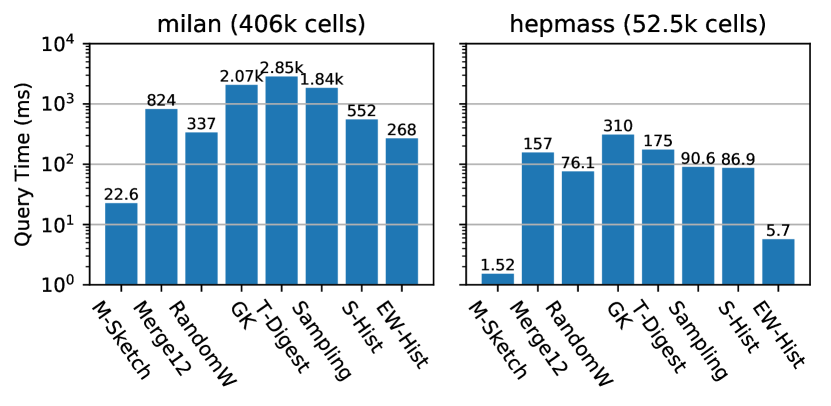
Figure 3. Total query time using different summaries to estimate quantiles with $\epsilon_{\mathrm{avg}}\leq.01$. The moments sketch enables significantly faster queries at this accuracy.

Figure 3 shows the total query time to merge the summaries and then compute a quantile estimate when each summary is instantiated at the smallest size sufficient to achieve $\epsilon_{\mathrm{avg}}\leq.01$ accuracy. We provide the parameters we used and average observed space usage in Table 2. On the long-tailed milan dataset, the S-Hist and EW-Hist summaries are unable to achieve $\epsilon_{\mathrm{avg}}\leq.01$ accuracy with less than 100 thousand buckets, so we provide timings at 100 buckets for comparison. The moments sketch provides $15$ to $50\times$ faster query times than RandomW, the next fastest accurate summary. As a baseline, sorting the milan dataset takes 7.0 seconds, selecting an exact quantile online takes 880ms, and streaming the data pointwise into a RandomW sketch with $\epsilon=1/40$ takes 220ms. These methods do not scale as well as using pre-aggregated moments sketches as dataset density grows but the number of cells remains fixed.

dataset	milan		hepmass
sketch	param	size (b)	param	size (b)
M-Sketch	$k=10$	200	$k=3$	72
Merge12	$k=32$	5920	$k=32$	5150
RandomW	$\epsilon=\frac{1}{40}$	3200	$\epsilon=\frac{1}{40}$	3375
GK	$\epsilon=\frac{1}{60}$	720	$\epsilon=\frac{1}{40}$	496
T-Digest	$\delta=5.0$	769	$\delta=1.5$	93
Sampling	1000 samples	8010	1000	8010
S-Hist	100 bins	1220	100	1220
EW-Hist	100 bins	812	15	132

Table 2. Summary size parameters used in Figure 3. We use these parameters to compare the query times at $\epsilon_{\mathrm{avg}}\leq.01$ accuracy.

6.2.2. Merge and Estimation Time

Recall that for a basic aggregate quantile query $t_{\mathrm{query}}=t_{\mathrm{merge}}\cdot n_{\mathrm{merge}}+t_{\mathrm{est}}.$ Thus we also measure $t_{\mathrm{merge}}$ and $t_{\mathrm{est}}$ to quantify the regimes where the moments sketch performs well. In these experiments, we vary the summary size parameters, though many summaries have a minimum size, and the moments sketch runs into numeric stability issues past $k\geq 15$ on some datasets (see Section 4.3.2).

In Figure 4 we evaluate the average time required to merge one of the cell summaries. Larger summaries are more expensive to merge, and the moments sketch has faster ($<50$ns) merge times throughout its size range. When comparing summaries using the parameters in Table 2, the moments sketch has up to $50\times$ faster merge times than other summaries with the same accuracy.

One can also parallelize the merges by sharding the data and having separate nodes operate over each partition, generating partial summaries to be aggregated into a final result. Since each parallel worker can operate independently, in these settings the moments sketch maintains the same relative performance improvements over alternative summaries when we can amortize fixed overheads, and we include supplemental parallel experiments in Appendix F in (Gan et al., 2018).

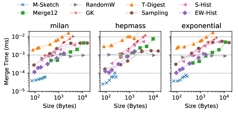
Figure 4. Per-merge latencies. The moments sketch provides faster merge times than alternative summaries at the same size.

The other major contributor to query time is estimation time. In Figure 5 we measure the time to estimate quantiles given an existing summary. The moments sketch provides on average 2 ms estimation times, though estimation time can be higher when our estimator chooses higher $k_{1},k_{2}$ to achieve better accuracy. This is the cause for the spike at $k=4$ in the milan dataset and users can can mitigate this by lowering the condition number threshold $\kappa_{\mathrm{max}}$. Other summaries support microsecond estimation times. The moments sketch thus offers a tradeoff of better merge time for worse estimation time. If users require faster estimation times, the cascades in Section 5.2 and the alternative estimators in Section 6.3 can assist.

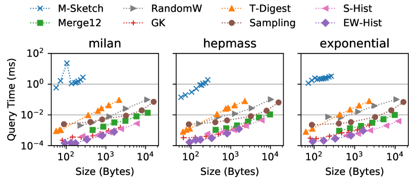
Figure 5. Quantile Estimation time. Estimation time on the moments sketch is slower than other sketches but under 3ms for $k=10$.

We show how the merge time and estimation time tradeoff define regimes where each component dominates depending on the number of merges. In Figure 6 we measure how the query time changes as we vary the number of summaries (cells of size 200) we aggregate. We use the moments sketch with $k=10$ and compare against the mergeable Merge12 and RandomW summaries with parameters from Table 2. When $n_{\mathrm{merge}}\geq 10^{4}$ merge time dominates and the moments sketch provides better performance than alternative summaries. However, the moments sketch estimation times dominate when $n_{\mathrm{merge}}\leq 100$.

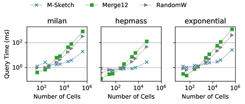
Figure 6. Comparing total query time using different mergeable summaries as we vary the number of merges. The moments sketch provides performance improvements when $n_{\mathrm{merge}}\geq 10^{4}$.

6.2.3. Accuracy

The moments sketch accuracy is dataset dependent, so in this section we compare the average quantile error on our evaluation datasets.

Figure 7 illustrates the average quantile error $\epsilon_{\mathrm{avg}}$ for summaries of different sizes constructed using pointwise accumulation on the complete dataset. The moments sketch achieves $\epsilon\leq 10^{-4}$ accuracy on the synthetic exponential dataset, and $\epsilon\leq 10^{-3}$ accuracy on the high entropy hepmass dataset. On other datasets it is able to achieve $\epsilon_{\mathrm{avg}}\leq 0.01$ with fewer than 200 bytes of space. On the integer retail dataset we round estimates to the nearest integer. The EW-Hist summary, while efficient to merge, provides less accurate estimates than the moments sketch, especially in the long-tailed milan and retail datasets.

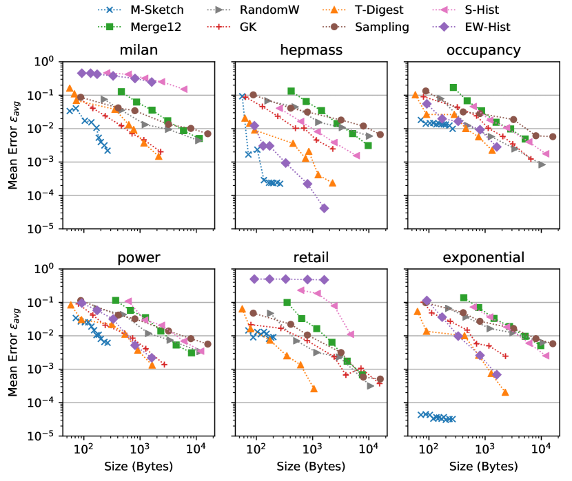
Figure 7. Average error for summaries of different sizes. The moments sketch delivers consistent $\epsilon_{\mathrm{avg}}\leq 0.015$ with fewer than 200 bytes.

We provide further experiments in (Gan et al., 2018) showing how the moments sketch worst-case error bounds are comparable to other summaries (Appendix E), that the moments sketch is robust to changes in skew and the presence of outliers (Appendix D), and that the moments sketch generalizes to a production workload (Appendix D.4). However, on datasets with low-entropy, in particular datasets consisting of a small number of discrete point masses, the maximum entropy principle provides poor accuracy. In the worst case, the maximum entropy solver can fail to converge on datasets with too few distinct values. Figure 8 illustrates how the error of the maximum entropy estimate increases as we lower the cardinality of a dataset consisting of uniformly spaced points in the range $[-1,1]$, eventually failing to converge on datasets with fewer than five distinct values. If users are expecting to run queries on primarily low-cardinality datasets, fixed-universe sketches or heavy-hitters sketches may be more appropriate.

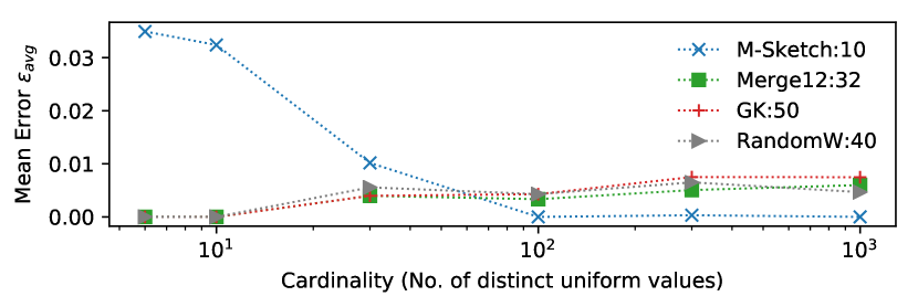
Figure 8. Accuracy of maximum entropy estimates on distributions with varying cardinality. The moments sketch is less accurate on discretized datasets, and fails to converge for cardinalities $n<5$.

6.3. Quantile Estimation Lesion Study

To evaluate each component of our quantile estimator design, we compare the accuracy and estimation time of a variety of alternative techniques on the milan and hepmass datasets. We evaluate the impact of using log moments, the maximum entropy distribution, and our optimizations to estimation.

Figure 9. Accuracy with and without log moments. Given the same total space budget, log moments improve accuracy on the long-tailed milan and retail datasets, and do not affect accuracy significantly on other datasets such as occupancy

To examine effectiveness of log moments, we compare our maximum entropy quantile estimator accuracy with and without log moments. For a fair comparison, we compare the estimates produced from $k$ standard moments and no log moments with those produced from up to $\frac{k}{2}$ of each. Figure 9 illustrates how on some long-tailed datasets, notably milan and retail, log moments reduce the error from $\epsilon>.15$ to $\epsilon<.015$. On other datasets, log moments do not have a significant impact.

We compare our estimator (opt) with a number of other estimators that make use of the same moments. The gaussian estimator fits a Gaussian distribution to the mean and standard deviation. The mnat estimator uses the closed form discrete CDF estimator in (Mnatsakanov, 2008). The svd estimator discretizes the domain and uses singular value decomposition to solve for a distribution with matching moments. The cvx-min estimator also discretizes the domain and uses a convex solver to construct a distribution with minimal maximum density and matching moments. The cvx-maxent estimator discretizes the domain and uses a convex solver to maximize the entropy, as described in Chapter 7 in (Boyd and Vandenberghe, 2004). The newton estimator implements our estimator without the integration techniques in Sec. 4.3, and uses adaptive Romberg integration instead (Press, 2007). The bfgs estimator implements maximum entropy optimization using the first-order L-BFGS (Liu and Nocedal, 1989) method as implemented in a Java port of liblbfgs (Khuc, 2017).

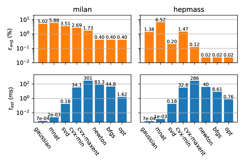
Figure 10. Lesion study comparing our optimized maximum entropy solver to other estimators. Our opt estimator provides at least $5\times$ less error than estimators that do not use maximum entropy, and up to $200\times$ faster estimation times than naive maximum entropy solvers.

Figure 10 illustrates the average quantile error and estimation time for these estimators. We run these experiments with $k=10$ moments. For uniform comparisons with other estimators, on the milan dataset we only use the log moments, and on the hepmass dataset we only use the standard moments. We perform discretizations using 1000 uniformly spaced points and make use of the ECOS convex solver (Domahidi et al., 2013). Solvers that use the maximum entropy principle provides at least $5\times$ less error than estimators that do not. Furthermore, our optimizations are able to improve the estimation time by a factor of up to $200\times$ over an implementation using generic solvers, and provide faster solve times than naive Newton’s method or BFGS optimizers. As described in Section 4.3, given the computations needed to calculate the gradient, one can compute the Hessian relatively cheaply, so our optimized Newton’s method is faster than BFGS.

7. Applying the Moments Sketch

In this section, we evaluate how the moments sketch affects performance when integrated with other data systems. We examine how the moments sketch improves query performance in the Druid analytics engine, as part of a cascade in the Macrobase feature selection engine (Bailis et al., 2017), and as part of exploratory sliding window queries.

7.1. Druid Integration

To illustrate the utility of the moments sketch in a modern analytics engine, we integrate the moments sketch with Druid (Yang et al., 2014). We do this by implementing moments sketch as an user-defined aggregation extension, and compare the total query time on quantile queries using the moments sketch with the default S-Hist summary used in Druid and introduced in (Ben-Haim and Tom-Tov, 2010). The authors in (Ben-Haim and Tom-Tov, 2010) observe on average 5% error for an S-Hist with 100 centroids, so we benchmark a moments sketch with $k=10$ against S-Hists with 10, 100, and 1000 centroids.

In our experiments, we deploy Druid on a single node – the same machine described in section 6.1 – with the same base configuration used in the default Druid quickstart. In particular, this configuration dedicates 2 threads to process aggregations. Then, we ingest 26 million entries from the milan dataset at a one hour granularity and construct a cube over the grid ID and country dimensions, resulting in 10 million cells.

Figure 11 compares the total time to query for a quantile on the complete dataset using the different summaries. The moments sketch provides $7\times$ lower query times than a S-Hist with 100 bins. Furthermore, as discussed in Section 6.2.1, any S-Hist with fewer than 10 thousand buckets provides worse accuracy on milan data than the moments sketch. As a best-case baseline, we also show the time taken to compute a native sum query on the same data. The 1 ms cost of solving for quantile estimates from the moments sketch on this dataset is negligible here.

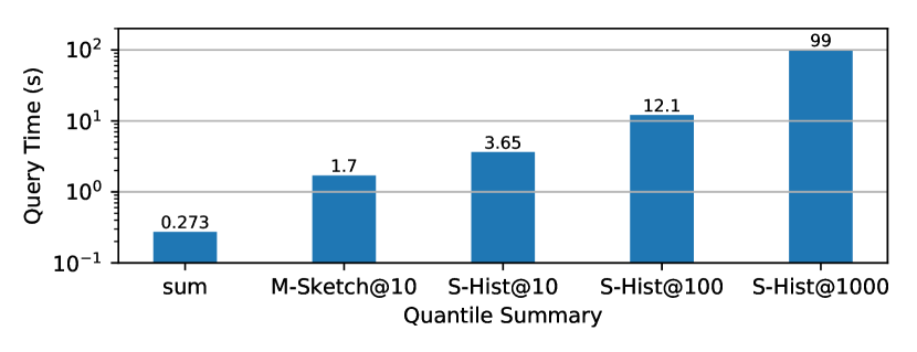
Figure 11. Druid end-to-end query benchmark. The moments sketch allows for faster query times than the comparable S-Hist summary with 100 bins. Runtime for a native sum operation is a lower bound on query time.

7.2. Threshold queries

In this section we evaluate how the cascades described in Section 5.2 improve performance on threshold predicates. First we show in Section 7.2.1 how the MacroBase analytics engine can use the moments sketch to search for anomalous dimension values. Then, we show in Section 7.2.2 how historical analytics queries can use the moments sketch to search and alert on sliding windows.

7.2.1. MacroBase Integration

The MacroBase engine searches for dimension values with unusually high outlier rates in a dataset (Bailis et al., 2017). For example, given an overall 2% outlier rate, MacroBase may report when a specific app version has an outlier rate of 20%. We integrate the moments sketch with a simplified deployment of MacroBase where all values greater than the global 99th percentile $t_{99}$ are considered outliers. We then query MacroBase for all dimension values with outlier rate at least $r=30\times$ greater than the overall outlier rate. This is equivalent to finding subpopulations whose 70th percentile is greater than $t_{99}$.

Given a cube with pre-aggregated moments sketches for each dimension value combination and no materialized roll-ups, MacroBase merges the moments sketches to calculate the global $t_{99}$, and then runs Algorithm 2 on every dimension-value subpopulation, searching for subgroups with $q_{.7}>t_{99}$. We evaluate the performance of this query on 80 million rows of the milan internet usage data from November 2013, pre-aggregated by grid ID, country, and at a four hour granularity. This resulted in 13 million cube cells, each with its own moments sketch.

Running the MacroBase query produces 19 candidate dimension values. We compare the total time to process this query using direct quantile estimates, our cascades, and the alternative Merge12 quantile sketch. In the first approach (Merge12a), we merge summaries during MacroBase execution as we do with a moments sketch. In the second approach (Merge12b), we calculate the number of values greater than the $t_{99}$ for each dimension value combination and accumulate these counts directly, instead of the sketches. We present this as an optimistic baseline, and is not always a feasible substitute for merging summaries.

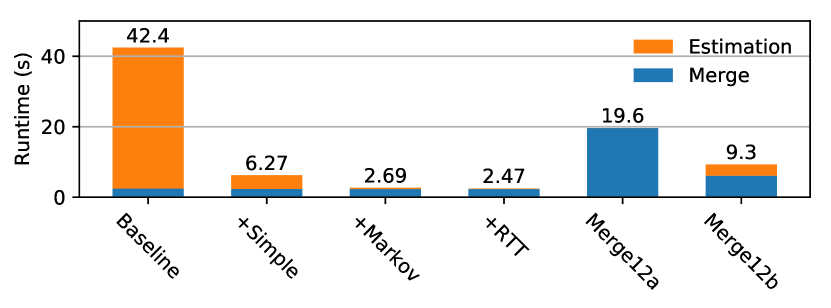
Figure 12. Runtime of MacroBase queries: the final moments sketch cascade outperforms queries using alternate sketches.

Figure 12 shows the query times for these different methods: the baseline method calculates quantile estimates directly, we show the effect of incrementally adding each stage of our cascade ending with +RTTBound. Each successive stage of the cascade improves query time substantially. With the complete cascade, estimation time is negligible compared to merge time. Furthermore, the moments sketch with cascades has $7.9\times$ lower query times than using the Merge12 sketch, and even $3.7\times$ lower query times than the Merge12b baseline.

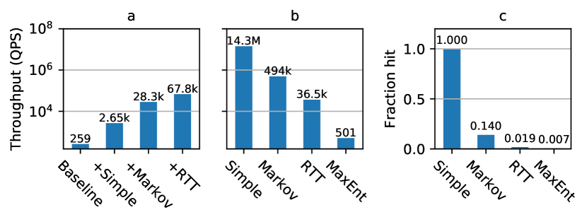
Figure 13. Cascades in MacroBase: (a) as we incrementally add cascade stages, threshold query throughput increases. (b) The cascade proceeds from faster to slower estimates. (c) Each stage of the cascade processes a smaller fraction of queries.

In Figure 13 we examine the impact the cascade has on estimation time directly. Each additional cascade stage improves threshold query throughput and is more expensive than the last. The complete cascade is over 250$\times$ faster than this baseline, and $25\times$ faster than just using a simple range check.

7.2.2. Sliding Window Queries

Threshold predicates are broadly applicable in data exploration queries. In this section, we evaluate how the moments sketch performs on sliding window alerting queries. This is useful when, for instance, users are searching for time windows of unusually high CPU usage spikes.

For this benchmark, we aggregated the 80 million rows of the milan dataset at a 10-minute granularity, which produced 4320 panes that spanned the month of November. We augmented the milan data with two spikes corresponding to hypothetical anomalies. Each spike spanned a two-hour time frame and contributed 10% more data to those time frames. Given a global 99th percentile of around 500 and a maximum value of 8000, we added spikes with values $x=2000$ and $x=1000$

We then queried for the 4-hour time windows whose 99th percentile was above a threshold $t=1500$. When processing this query using a moments sketch, we can update sliding windows using turnstile semantics, subtracting the values from the oldest pane and merging in the new one, and use our cascade to filter windows with quantiles above the threshold.

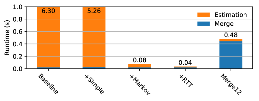
Figure 14. Sliding window query: moments sketch with cascades runs 13$\times$ faster than Merge12.

Figure 14 shows the runtime of the sliding window query using both the moments sketch and Merge12. Faster moments sketch merge times and the use of turnstile semantics then allow for 13$\times$ faster queries than Merge12.

8. Conclusion

In this paper, we show how to improve the performance of quantile aggregation queries using statistical moments. Low merge overhead allows the moments sketch to outperform comparably accurate existing summaries when queries aggregate more than 10 thousand summaries. By making use of the method of moments and the maximum entropy principle, the moments sketch provides $\epsilon_{\mathrm{avg}}\leq 0.01$ accuracy on real-world datasets, while the use of numeric optimizations and cascades keep query times at interactive latencies.

Appendix A Maximum Entropy Estimation

A.1. Newton’s Method Details

Recall that we wish to solve the following optimization problem:

$$\underset{f\in\mathcal{F}[x_{\mathrm{min}},x_{\mathrm{max}}]}{\mathrm{maximize}} H[f]$$

subject to $$\int_{x_{\mathrm{min}}}^{x_{\mathrm{max}}}x^{i}f(x)\,dx=\mu_{i}, i\in\{1,\dots,k_{1}\}$$

$$\int_{x_{\mathrm{min}}}^{x_{\mathrm{max}}}\log^{i}(x)f(x)\,dx=\nu_{i}, i\in\{1,\dots,k_{2}\}$$

.

Throughout this section it is easier to reformulate this problem in more general terms, using the functions

(8) $$m_{i}(x)=\begin{cases}x^{i}&0\leq i\leq k_{1}\\ h(x)^{i-k_{1}}&k_{1}+1\leq i\leq k_{1}+k_{2}.\end{cases}$$

where $h(x)=\log(x)$ or $h(x)=e^{x}$ depending on whether we work using the $x$ or log-transformed $x^{\prime}=\log(x)$ as our primary metric. Letting $k_{t}=k_{1}+k_{2}$, and folding the $\nu_{i}$ into a larger $\vec{\mu}$ vector, our optimization problem is then:

(9) $$\underset{f\in\mathcal{F}[x_{\mathrm{min}},x_{\mathrm{max}}]}{\mathrm{maximize}} H[f]$$

subject to $$\int_{x_{\mathrm{min}}}^{x_{\mathrm{max}}}m_{i}(x)f(x)\,dx=\mu_{i}, i\in\{0,\dots,k_{t}\}$$

.

Functional analysis (Jaynes, 1957) tells us that a maximal entropy solution to Eq. (9) has the form:

$$f(x;\theta)=\exp\left(\sum_{i=0}^{k_{t}}\theta_{i}m_{i}(x)\right),$$

Then if we define the potential function $L(\theta)$ from (Mead and Papanicolaou, 1984):

(10) $$L(\theta)= \int_{x_{\mathrm{min}}}^{x_{\mathrm{min}}}\exp\left(\sum_{i=0}^{k_{t}}\theta_{i}m_{i}(x)\right)-\sum_{i=0}^{k_{t}}\theta_{i}\mu_{i}$$

We can calculate the gradient and Hessian of $L(\theta)$ as follows:

(11) $$\frac{\partial L}{\partial\theta_{i}}=\int_{x_{\mathrm{min}}}^{x_{\mathrm{min}}}m_{i}(x)\exp{\left(\sum_{i=0}^{k_{t}}\theta_{i}m_{i}(x)\right)}-\mu_{i}$$

(12) $$\frac{\partial^{2}\Gamma}{\partial\theta_{i}\partial\theta_{j}}=\int_{x_{\mathrm{min}}}^{x_{\mathrm{min}}}m_{i}(x)m_{j}(x)\exp{\left(\sum_{i=0}^{k_{t}}\theta_{i}m_{i}(x)\right)}$$

Note that when the gradient given in Eq. (11) is zero then the constraints in Eq. (9) are satisfied. Since $L(\theta)$ is convex and has domain $\mathbb{R}^{k_{d}}$, this means that by solving the unconstrained minimization problem over $L(\theta)$ we can find a solution $\theta$ we can find a solution to the constrained maximum entropy problem. Since Newton’s method is a second order method, we can use Equations (10), (11), (12) are to execute Newton’s method with backtracking line search (Boyd and Vandenberghe, 2004).

A.2. Practical Implementation Details

Chebyshev Polynomial Basis Functions.

As described in Section 4.3, we can improve the stability of our optimization problem by using Chebyshev polynomials. To do so, we must redefine our $m_{i}(x)$

$$m_{i}(x)=\begin{cases}T_{i}(s_{1}(x)),&i\in\{1,\dots,k_{1}\}\\ T_{i-k_{1}}(s_{2}(h(x))),&i\in\{k_{1}+1,\dots,k_{1}+k_{2}\}\end{cases}$$

where $T_{i}(x)$ are Chebyshev polynomials of the first kind (Press, 2007) and the $s_{1},s_{2}$ are linear scaling functions to map onto $[-1,1]$ defined as:

$$s_{1}(x) =\left(x-\frac{x_{\mathrm{max}}+x_{\mathrm{min}}}{2}\right)/\left(\frac{x_{\mathrm{max}}-x_{\mathrm{min}}}{2}\right)$$

$$s_{2}(x) =\left(x-\frac{h(x_{\mathrm{max}})+h(x_{\mathrm{min}})}{2}\right)/\left(\frac{h(x_{\mathrm{max}})-h(x_{\mathrm{min}})}{2}\right).$$

The formulae for $\mu_{i},\Gamma,\nabla\Gamma,\nabla^{2}\Gamma$ still hold, but now the $\mu_{i}$ are

(13) $$\mu_{i}=\frac{1}{n}\begin{cases}\sum_{x}T_{i}(s_{1}(x))&0\leq i\leq k_{1}\\ \sum_{x}T_{i-k_{a}}(s_{2}(h(x)))&k_{1}+1\leq i\leq k_{1}+k_{2}.\end{cases}.$$

These can be computed from the quantities $\mu_{i}=\sum_{x}x^{i}$, $\nu_{i}=\sum_{x}h(x)^{i}$ originally stored in the moments sketch by using the binomial expansion and standard formulae for expressing Chebyshev polynomials in terms of standard monomials (Mason and Handscomb, 2002).

Chebyshev Polynomial Integration.

In this section we will show how Chebyshev approximation provides for efficient ways to compute the gradient and Hessian. Here it is easier to work with the change of variables $u=s_{1}(x)$ so that $f^{u}(u)=f(s_{1}^{-1}(u))$ has domain $[-1,1]$. First, we will examine the case when $k_{2}=0$. If we can approximate $f(u;\theta)$ as a linear combination of chebyshev polynomials:

(14) $$f^{u}(u;\theta) =\exp\left(\sum_{i=0}^{k_{t}}\theta_{i}m_{i}(u)\right)$$

(15) $$\approx\sum_{j=0}^{n_{c}}c_{j}T_{j}(u)$$

Then using polynomial identities such as $T_{i}(x)T_{j}(x)=\frac{1}{2}(T_{i+j}(x)+T_{|i-j|}(x))$ we can evaluate the Gradient and Hessian in Eqs. (11), (12) using $O(k_{1}n_{c})$ algebraic operations.

We can approximate $f^{u}(u;\theta)$ using the Clenshaw Curtis quadrature formulas to approximate a function $f$ supported on $[-1,1]$ (Eq. 5.9.4 in (Press, 2007)):

(16) $$a_{j}=\frac{2}{n_{c}}\left(\frac{f(1)}{2}-\frac{f(-1)}{2}+\sum_{i=1}^{n_{c}-1}f\left[\cos\left(\frac{\pi i}{n_{c}}\right)\right]\cos\left(\frac{\pi i}{n_{c}}\right)\right)$$

Then

(17) $$f(x)\approx\frac{1}{2}T_{0}(x)+\sum_{i=1}^{n_{c}}a_{i}T_{i}(x)$$

where Eq. (16) can be evaluated in $n_{c}\log{n_{c}}$ time using the Fact Cosine Transform (Press, 2007). The case when $k_{2}>0$ is similar except we need to approximate not just $f^{u}(u;\theta)$ but also $T_{i}(s_{2}(h(s_{1}^{-1}(u)))f^{u}(u;\theta)$ for $i\leq k_{2}$.

Appendix B Numeric Stability of Moments

As mentioned in Section 4.3.2, floating point arithmetic limits the usefulness of higher moments. This is because the raw moments $\frac{1}{n}\sum x^{i}$ are difficult to optimize over and analyze: both maximum entropy estimation (Section 4.3) and theoretical error bounds (Section 4.4) apply naturally to moments on data in the range $[-1,1]$. In particular, shifting the data improves the conditoning of the optimization problem dramatically. However, when merging sketches from different datasets, users may not know the full range of the data ahead of time, so the power sums stored in a moments sketch correspond to data in an arbitrary range $[a,b]$. Thus, we will analyze how floating point arithmetic affects the process of scaling and shifting the data so that it is supported in the range $[-1,1]$. This is similar to the process of calculating a variance by shifting the data so that it is centered at zero.

We can calculate the moments of scaling data $x_{scale}=k\cdot x$ with error only in the last digit, so we can assume we have data in the range $[c-1,c+1]$. Let $\mu_{i}$ be the moments of the $x_{scale}$, and let $\mu_{i}^{s}$ be the moments of the shifted data $x_{shift}=x_{scale}-c$. Using the binomial expansion

$$\mu_{k}^{s} =\frac{1}{n}\sum_{x\in x_{scale}}\left(x-c\right)^{k}$$

$$=\sum_{i=0}^{k}{k\choose i}\mu_{i}(-c)^{k-i}$$

Using numerically stable addition, we can calculate $\mu_{k}$ to a relative precision $\delta$ close to machine precision $\delta\approx 2^{-53}$. Then, the absolute error $\delta_{k}$ in estimating $\mu_{k}^{s}$ is bounded by:

$$\delta_{k} \leq\sum_{i=0}^{k}{k\choose i}|\mu_{i}||c|^{k-i}\delta$$

$$\delta_{k} \leq\sum_{i=0}^{k}{k\choose i}(|c|+1)^{k}\delta$$

$$\leq 2^{k}(|c|+1)^{k}\delta$$

We know that the average quantile error (Equation 7 in Section 4.4) is bounded by

$$\epsilon_{\textrm{avg}}\leq O\left(\frac{1}{k}+3^{k}\|\mu_{f}-\mu_{\hat{f}}\|_{2}\right),$$

so if we can calculate all of the $\mu_{i}^{s}$ to within precision $3^{-k}\left(\frac{1}{k-1}-\frac{1}{k}\right)$ then we have enough precision to bound the quantile estimate by $O\left(\frac{1}{k-1}\right)$. This way, we can show that the error bound from using the first $k$ moments will be at least as tight as the bound from using the first $k-1$ moments. As $k$ and $|c|$ grow, achieving this precision becomes more and more difficult, and we can solve for the cutoff point using base-10 $\log$.

(18) $$2^{k}(|c|+1)^{k}\delta \leq 3^{-k}\left(\frac{1}{k-1}-\frac{1}{k}\right)$$

(19) $$k\left(\log{6}+\log{(|c|+1)}\right) \leq\log{\frac{1}{\delta}}-\log{(k^{2}-k)})$$

Plugging in double precision for $\delta$ into Eq. (19), we know that $k\leq\frac{53\log{2}}{\log{6}}\leq 20$, so $\log{(k^{2}-k)}\leq 2.58$

(20) $$k \leq\frac{53\log{2}-2.58}{\log{6}+\log{(|c|+1)}}$$

(21) $$\leq\frac{13.35}{.78+\log{(|c|+1)}}$$

Equation 21 is a conservative bound on the number of numerically stable moments we can extract from an moments sketch, and suggests that when our data is centered at 0, we have at least $17$ stable moments. When the raw data have range $[x_{\mathrm{min}},3x_{\mathrm{min}}]$, then $c=2$, and we have at least $10$ stable moments. In our evaluations, $10$ stable moments are enough to achieve quantile error $\approx.01$. Figure 15 describes how the bound in Equation 21 varies with $c$, and compares it with the highest order stable moment of a uniform distribution supported on $[c-1,c+1]$. This confirms that our formula is a conservative bound on the true precision loss due to the shift. If the raw data are centered even further from 0, users can consider pre-shifting all of their data to make better use of numeric precision.

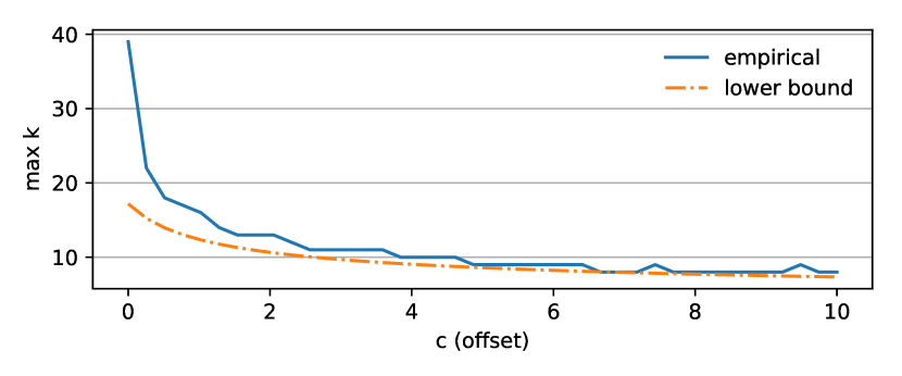
Figure 15. Highest order usable moments for data centered at different locations. Our data-independent bound is conservative compared to values on a uniform dataset.

As a measure of the downstream impact of this effect on some of our evaluation datasets, Figure 16 shows the precision loss during Chebyshev polynomial calculation $\Delta\mu=|\mu_{i}-\hat{\mu}_{i}|$ where $\mu_{i}$ is the true Chebyshev moment and $\hat{\mu}_{i}$ is the value calculated from the moments sketch. Precision loss is more severe on the occupancy dataset which is centered away from zero ($c\approx 1.5$) compared with the hepmass dataset ($c\approx 0.4$). See Table 1.

Figure 16. Precision loss from shifting and converting higher moments to chebyshev moments. The occupancy dataset exhibits more precision loss because it is centered further away from zero.

Appendix C Low-precision storage

In Appendix B we discussed how floating point precision limits the usability of higher moments. Conversely, in settings where space is heavily constrained, the data is well-centered, and we only need a limited number of moments, the moments sketch can be compressed by reducing the precision of the sketch contents using randomized rounding.

As a proof-of-concept of this approach, we created an encoder that compresses the double precision floating point values in a moments sketch using reduced floating point precision, quantizing the significand and removing unused bits in the exponent. This low-precision representation has a negligible impact on merge times since we can convert them to and from native double precision using simple bit manipulation.

We evaluate the encoding by constructing 100 thousand pre-aggregated moments sketches, reducing their precision, and then merging them and querying for quantiles on the aggregation. Figure 17 illustrates how the quality of the final estimate remains stable as the precision is decreased until we reach a minimum threshold, after which accuracy degrades. On the milan dataset, a moments sketch with $k=10$ can be stored with 20 bits per value without noticeably affecting our quantile estimates, representing a $3\times$ space reduction compared to standard double precision floating point.

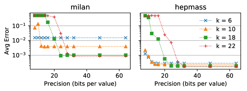
Figure 17. Average error for low-precision moments sketches after 100 thousand merges. Twenty bits of precision is sufficient to maintain accuracy for both datasets.

These results are consistent with the bounds in Section B and show how higher moments require more bits of precision. However, the bounds are conservative since they only consider the midpoint $c$ of a dataset and are otherwise both dataset-independent and agnostic to the maximum entropy principle.

Appendix D Additional Workloads

The moments sketch accuracy and performance generalizes across a range of workloads. In this section we evaluate its performance on datasets with varying skew, in the presence of outlier values, under a coarser pre-aggregation policy, and on a production workload.

D.1. Data Skew

Our usage of log-moments greatly reduces the impact of data skew on the accuracy of moments sketch quantile estimates. In Figure 18 we vary the shape parameter $k_{s}$ of a Gamma distribution with scale factor $\theta=1$. The skew of this distribution is $\frac{2}{\sqrt{k_{s}}}$ so $k_{s}=0.1$ corresponds to very high skew. For $k_{s}=0.1,1.0,10.0$, our estimator can achieve $\epsilon_{avg}\leq 10^{-3}$ error. The accuracy regressions on orders $3$ and $7$ occur when the solver stops making use of all available moments to reduce the condition number of the Hessian (Section 4.3). In this specific case, our solver uses a heuristic to decide that given a maximum condition number, optimizing using 3 log moments is more valuable than 2 log moments and 2 standard moments. This choice leads to worse accuracy on a Gamma distribution, but in general it is difficult to know which subset of moments will yield the most accurate estimate. More effective heuristics for choosing subsets of moments that do not exceed a condition number threshold is an open direction for future research.

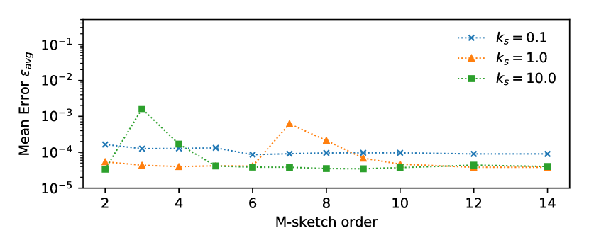
Figure 18. Accuracy of estimates on Gamma distributions with varying shape parameter $k_{s}$. The maximum entropy principle is able to construct an accurate estimate across a range of parameters.

D.2. Outlier Values

The moments sketch, unlike histogram-based sketches, is also somewhat robust to the presence of large outlier values in a dataset. In Figure 19 we evaluate the effect of adding a fixed fraction $\delta=0.01$ of outlier values from a Gaussian with mean $\mu_{o}$ and standard deviation $\sigma=0.1$ to a dataset of 10 million standard Gaussian points. As we increase the magnitude $\mu_{o}$ of the outliers, the EW-Hist summaries with 20 and 100 bins lose accuracy though a moments sketch with $k=10$ remains accurate. The Merge12 sketch is agnostic to value magnitudes and is unaffected by the outliers. If extremely large outliers are expected, floating point precision suffers and the moments sketch can be used in conjunction with standard outlier removal techniques.

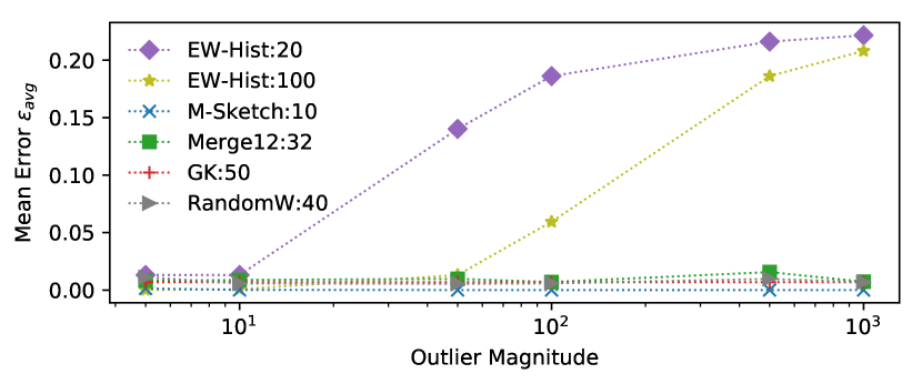
Figure 19. Mean error on a Gaussian dataset with outliers of different magnitudes added. The moments sketch remains accurate for large outliers, but the EW-Hist accuracy degrades.

D.3. Varying Aggregation

In our main evaluations, we group our datasets into cells of 200 elements and construct sketches for each cell to maintain a pre-aggregated collection of data summaries. We do not target deployments where very few elements can be pre-aggregated per summary: in these cases merging moments sketches is relatively expensive. On the other hand production data systems can have much larger data volumes and opportunities to pre-aggregate more elements per cell. Since the moments sketch is fixed-size regardless of the data, increasing the number of elements per cell does not affect its merge time performance, while other sketches which which have not reached their maximum capacity will be correspondingly larger and slower to merge.

In Figure 20 we measure the time taken per merge for different summaries constructed on cells of 2000 elements for the milan, hepmass, and exponential dataset, and cells of 10000 elements on a synthetic Gaussian dataset with 1 billion points. The relative performance of different sketches matches closely with Figure 4, except that larger Sampling and Merge12 summaries are now slower when constructed on more than 200 elements.

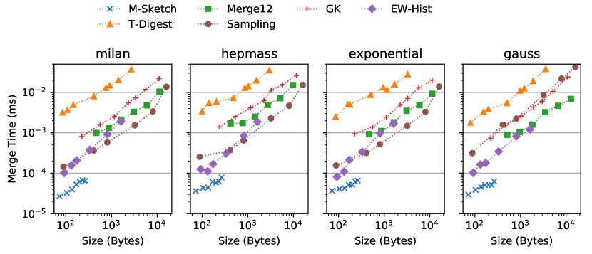
Figure 20. Merge times on with sketches on cells of 2000 elements, and on a Gaussian dataset with cells of 10000 elements. Since the moments sketch has a fixed size, its per-merge times remain faster than alternative sketches with comparable accuracy.

D.4. Production workload

In this section we evaluate merge time and accuracy on a production workload from Microsoft that contains 165 million rows of application telemetry data for an integer-valued performance metric. We group and pre-aggregate based on four columns that encode information about application version, network type, location, and time, resulting in 400 thousand cells. Notably, these cells do not correspond to equal sized partitions, but have a minimum size of 5 elements, a maximum size of 722044 elements, and an average size of 2380 elements. Figure 21 illustrates the distribution of integer data values and the cell sizes.

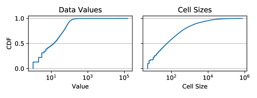
Figure 21. Microsoft data values and cell sizes.

Then, we measure the performance and accuracy of merging the cells to perform a quantile aggregation query. Figure 22 illustrates that on this workload with variable sized cells, the moments sketch still provides faster merge times than comparably accurate summaries (c.f. Appendix D.3). The moments sketch achieves $\epsilon_{avg}<.01$ error when we round estimates to the nearest integer on this integral dataset. Since the GK sketch is not strictly mergeable (Agarwal et al., 2012), it grows considerably when merging the heterogenous summaries in this workload to preserve its accuracy.

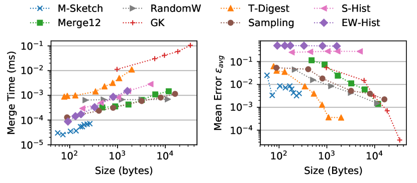
Figure 22. Merge times and accuracy on the Microsoft dataset. The merge performance of the moments sketch generalizes to workloads with variable sized cells, and exhibits an error rate of $\epsilon_{avg}<.01$.

Appendix E Error Upper Bounds

Thus far we have evaluated observed accuracy. For comparison, Figure 23 shows the average guaranteed upper bound error provided by different summaries constructed using pointwise accumulation on the datasets (no merging). These are in general higher than the observed errors. We use the RTTBound routine in Section 5.1 to bound the moments sketch error. We omit the S-Hist since it does not provide upper bounds. When merging is not a concern, the GK summary provides the best guaranteed error.

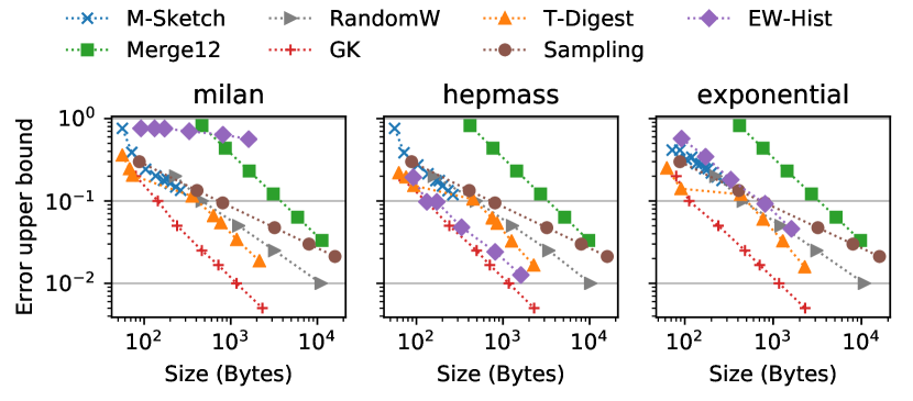
Figure 23. Average bound size for summaries of different sizes. No summary is able to provide $\epsilon_{bound}\leq.01$ guarantees with less than 1000 bytes.

Appendix F Parallel Merges

In Section 6.2.1, we evaluated merge time through single-threaded experiments. We evaluate how well throughput generalizes to parallel aggregation by sharding pre-computed summaries into equal sized batches, and merging the summaries in each batch on an independent worker thread. After all threads have completed, we combine the merged result from each batch using a sequential merge to obtain a final summary for the complete dataset.

In Figure 24 we evaluate strong scalability by measuring the total throughput in merging 400 thousand summaries (constructed from blocks of 200 elements) as we increase the number of threads. In our experiments we needed to duplicate the hepmass dataset to yield 400 thousand summaries, and initialized summaries using the parameters in Table 2. The moments sketch remains faster than alternate summaries as we increase the amount of parallelism, though thread overheads and variance in stragglers limits parallelism on these datasets past 8 threads when there is less work per thread. In Figure 25 we evaluate weak scalability by performing a similar experiment but increase the dataset size alongside thread count, keeping number of merges per thread constant. Under these conditions, the moments sketch and other summaries achieve even better scalability.

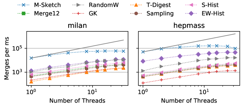
Figure 24. Strong scaling of parallel merging. For fixed number of merges, the throughput of the moments sketch scales with the number of threads available up to 8-way parallelism, and remains faster than alternatives. The solid line shows ideal moments sketch scaling.

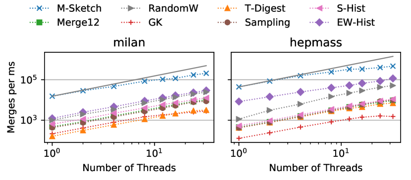
Figure 25. Weak scaling of parallel merging. For fixed number of merges per thread, the moments sketch and other summaries scale nearly linearly with parallelism.

These experiments confirm our intuition that since merges can be performed independently, single-threaded performance is indicative of parallel performance, and the relative speedup provided by the moments sketch remains stable in parallel settings. The moments sketch and other summaries can be used in more sophisticated distributed aggregation plans as well, such as in (Rusu and Dobra, 2012; Budiu et al., 2016), though since the moments sketch is so compact and cheap to merge, multi-level hierarchical aggregation is only profitable when enormous numbers of cores are available.

References

- (1)
- dat (2017) 2017. Yahoo! Data Sketches Library. https://datasketches.github.io/.
- Abraham et al. (2013) Lior Abraham, John Allen, Oleksandr Barykin, Vinayak Borkar, Bhuwan Chopra, Ciprian Gerea, Daniel Merl, Josh Metzler, David Reiss, Subbu Subramanian, Janet L. Wiener, and Okay Zed. 2013. Scuba: Diving into Data at Facebook. VLDB 6, 11 (2013), 1057–1067.
- Agarwal et al. (2012) Pankaj K. Agarwal, Graham Cormode, Zengfeng Huang, Jeff Phillips, Zhewei Wei, and Ke Yi. 2012. Mergeable Summaries. In PODS.
- Agarwal et al. (2013) Sameer Agarwal, Barzan Mozafari, Aurojit Panda, Henry Milner, Samuel Madden, and Ion Stoica. 2013. BlinkDB: Queries with Bounded Errors and Bounded Response Times on Very Large Data. In EuroSys. 29–42.
- Akhiezer (1965) N.I. Akhiezer. 1965. The Classical Moment Problem and Some Related Questions in Analysis. Oliver & Boyd.
- Ambrosio et al. (2008) Luigi Ambrosio, Nicola Gigli, and Giuseppe Savaré. 2008. Gradient flows: in metric spaces and in the space of probability measures. Springer Science & Business Media.
- Anandkumar et al. (2012) Animashree Anandkumar, Daniel Hsu, and Sham M Kakade. 2012. A method of moments for mixture models and hidden Markov models. In COLT. 33–1.
- Bailis et al. (2017) Peter Bailis, Edward Gan, Samuel Madden, Deepak Narayanan, Kexin Rong, and Sahaana Suri. 2017. MacroBase: Prioritizing attention in fast data. In SIGMOD. 541–556.
- Balestrino et al. (2003) A. Balestrino, A. Caiti, A. Noe’, and F. Parenti. 2003. Maximum entropy based numerical algorithms for approximation of probability density functions. In 2003 European Control Conference (ECC). 796–801.
- Bandyopadhyay et al. (2005) K. Bandyopadhyay, A. K. Bhattacharya, Parthapratim Biswas, and D. A. Drabold. 2005. Maximum entropy and the problem of moments: A stable algorithm. Phys. Rev. E 71 (May 2005), 057701. Issue 5.
- Belkin and Sinha (2010) Mikhail Belkin and Kaushik Sinha. 2010. Polynomial Learning of Distribution Families. In FOCS. 10.
- Ben-Haim and Tom-Tov (2010) Yael Ben-Haim and Elad Tom-Tov. 2010. A streaming parallel decision tree algorithm. Journal of Machine Learning Research 11, Feb (2010), 849–872.
- Berger et al. (1996) Adam L Berger, Vincent J Della Pietra, and Stephen A Della Pietra. 1996. A maximum entropy approach to natural language processing. Computational linguistics 22, 1 (1996), 39–71.
- Beyer et al. (2016) B. Beyer, C. Jones, J. Petoff, and N.R. Murphy. 2016. Site Reliability Engineering: How Google Runs Production Systems. O’Reilly Media, Incorporated.
- Boyd and Vandenberghe (2004) Stephen Boyd and Lieven Vandenberghe. 2004. Convex Optimization. Cambridge University Press, New York, NY, USA.
- Braun et al. (2015) Lucas Braun, Thomas Etter, Georgios Gasparis, Martin Kaufmann, Donald Kossmann, Daniel Widmer, Aharon Avitzur, Anthony Iliopoulos, Eliezer Levy, and Ning Liang. 2015. Analytics in Motion: High Performance Event-Processing AND Real-Time Analytics in the Same Database. In SIGMOD. 251–264.
- Budiu et al. (2016) Mihai Budiu, Rebecca Isaacs, Derek Murray, Gordon Plotkin, Paul Barham, Samer Al-Kiswany, Yazan Boshmaf, Qingzhou Luo, and Alexandr Andoni. 2016. Interacting with Large Distributed Datasets Using Sketch. In Eurographics Symposium on Parallel Graphics and Visualization.
- Buragohain and Suri (2009) Chiranjeeb Buragohain and Subhash Suri. 2009. Quantiles on streams. In Encyclopedia of Database Systems. Springer, 2235–2240.
- Chen et al. (2006) Yixin Chen, Guozhu Dong, Jiawei Han, Jian Pei, Benjamin W Wah, and Jianyong Wang. 2006. Regression cubes with lossless compression and aggregation. TKDE 18, 12 (2006), 1585–1599.
- Cohen (2006) Sara Cohen. 2006. User-defined aggregate functions: bridging theory and practice. In SIGMOD. 49–60.
- Cormode and Garofalakis (2007) Graham Cormode and Minos Garofalakis. 2007. Streaming in a connected world: querying and tracking distributed data streams. In SIGMOD. 1178–1181.
- Cormode et al. (2012) Graham Cormode, Minos Garofalakis, Peter J Haas, and Chris Jermaine. 2012. Synopses for massive data: Samples, histograms, wavelets, sketches. Foundations and Trends in Databases 4, 1–3 (2012), 1–294.
- Cormode and Muthukrishnan (2005) Graham Cormode and S. Muthukrishnan. 2005. An Improved Data Stream Summary: The Count-min Sketch and Its Applications. J. Algorithms 55, 1 (April 2005), 58–75.
- Cranor et al. (2003) Chuck Cranor, Theodore Johnson, Oliver Spataschek, and Vladislav Shkapenyuk. 2003. Gigascope: A Stream Database for Network Applications. In SIGMOD. 647–651.
- Datar et al. (2002) Mayur Datar, Aristides Gionis, Piotr Indyk, and Rajeev Motwani. 2002. Maintaining stream statistics over sliding windows. SIAM journal on computing 31, 6 (2002), 1794–1813.
- Dean and Barroso (2013) Jeffrey Dean and Luiz André Barroso. 2013. The Tail at Scale. Commun. ACM 56, 2 (2013), 74–80.
- Domahidi et al. (2013) A. Domahidi, E. Chu, and S. Boyd. 2013. ECOS: An SOCP solver for embedded systems. In European Control Conference (ECC). 3071–3076.
- Dunning and Ertl (2017) Ted Dunning and Otmar Ertl. 2017. Computing extremeley accurate quantiles using t-digests. https://github.com/tdunning/t-digest.
- Feng et al. (2015) W. Feng, C. Zhang, W. Zhang, J. Han, J. Wang, C. Aggarwal, and J. Huang. 2015. STREAMCUBE: Hierarchical spatio-temporal hashtag clustering for event exploration over the Twitter stream. In ICDE. 1561–1572.
- Gan et al. (2018) Edward Gan, Jialin Ding, Kai Sheng Tai, Vatsal Sharan, and Peter Bailis. 2018. Moment-Based Quantile Sketches for Efficient High Cardinality Aggregation Queries. Technical Report. Stanford University. http://arxiv.org/abs/1803.01969
- Gautschi (1978) Walter Gautschi. 1978. Questions of Numerical Condition Related to Polynomials. In Recent Advances in Numerical Analysis, Carl De Boor and Gene H. Golub (Eds.). Academic Press, 45 – 72.
- Gibson (2014) Walton C Gibson. 2014. The method of moments in electromagnetics. CRC press.
- Gray et al. (1997) Jim Gray, Surajit Chaudhuri, Adam Bosworth, Andrew Layman, Don Reichart, Murali Venkatrao, Frank Pellow, and Hamid Pirahesh. 1997. Data cube: A relational aggregation operator generalizing group-by, cross-tab, and sub-totals. Data mining and knowledge discovery 1, 1 (1997), 29–53.
- Greenwald and Khanna (2001) Michael Greenwald and Sanjeev Khanna. 2001. Space-efficient online computation of quantile summaries. In SIGMOD, Vol. 30. 58–66.
- Hall et al. (2016) Alex Hall, Alexandru Tudorica, Filip Buruiana, Reimar Hofmann, Silviu-Ionut Ganceanu, and Thomas Hofmann. 2016. Trading off Accuracy for Speed in PowerDrill. In ICDE. 2121–2132.
- Hansen (1982) Lars Peter Hansen. 1982. Large sample properties of generalized method of moments estimators. Econometrica (1982), 1029–1054.
- Harinarayan et al. (1996) Venky Harinarayan, Anand Rajaraman, and Jeffrey D. Ullman. 1996. Implementing Data Cubes Efficiently. In SIGMOD. 205–216.
- Hill et al. (2017) Daniel N. Hill, Houssam Nassif, Yi Liu, Anand Iyer, and S.V.N. Vishwanathan. 2017. An Efficient Bandit Algorithm for Realtime Multivariate Optimization. In KDD. 1813–1821.
- Hunter et al. (2016) Tim Hunter, Hossein Falaki, and Joseph Bradley. 2016. Approximate Algorithms in Apache Spark: HyperLogLog and Quantiles. https://databricks.com/blog/2016/05/19/approximate-algorithms-in-apache-spark-hyperloglog-and-quantiles.html.
- Italia (2015) Telecom Italia. 2015. Telecommunications - SMS, Call, Internet - MI. https://doi.org/10.7910/DVN/EGZHFV http://dx.doi.org/10.7910/DVN/EGZHFV.
- Jaynes (1957) E. T. Jaynes. 1957. Information Theory and Statistical Mechanics. Phys. Rev. 106 (May 1957), 620–630. Issue 4.
- Johari et al. (2017) Ramesh Johari, Pete Koomen, Leonid Pekelis, and David Walsh. 2017. Peeking at A/B Tests: Why It Matters, and What to Do About It. In KDD. 1517–1525.
- Kalai et al. (2010) Adam Tauman Kalai, Ankur Moitra, and Gregory Valiant. 2010. Efficiently learning mixtures of two Gaussians. In STOC. 553–562.
- Kamat et al. (2014) N. Kamat, P. Jayachandran, K. Tunga, and A. Nandi. 2014. Distributed and interactive cube exploration. In IDCE. 472–483.
- Kempe et al. (2003) David Kempe, Alin Dobra, and Johannes Gehrke. 2003. Gossip-based computation of aggregate information. In FOCS. 482–491.
- Khuc (2017) Vinh Khuc. 2017. lbfgs4j. https://github.com/vinhkhuc/lbfgs4j https://github.com/vinhkhuc/lbfgs4j.
- Kong and Valiant (2017) Weihao Kong and Gregory Valiant. 2017. Spectrum estimation from samples. Ann. Statist. 45, 5 (10 2017), 2218–2247.
- Lafferty et al. (2001) John D. Lafferty, Andrew McCallum, and Fernando C. N. Pereira. 2001. Conditional Random Fields: Probabilistic Models for Segmenting and Labeling Sequence Data. In ICML. 282–289.
- Lichman (2013) M. Lichman. 2013. UCI Machine Learning Repository. http://archive.ics.uci.edu/ml
- Liu and Nocedal (1989) Dong C. Liu and Jorge Nocedal. 1989. On the limited memory BFGS method for large scale optimization. Mathematical Programming 45, 1 (Aug 1989), 503–528.
- Liu et al. (2016) Shaosu Liu, Bin Song, Sriharsha Gangam, Lawrence Lo, and Khaled Elmeleegy. 2016. Kodiak: Leveraging Materialized Views for Very Low-latency Analytics over High-dimensional Web-scale Data. VLDB 9, 13 (2016), 1269–1280.
- Luo et al. (2016) Ge Luo, Lu Wang, Ke Yi, and Graham Cormode. 2016. Quantiles over data streams: experimental comparisons, new analyses, and further improvements. VLDB 25, 4 (2016), 449–472.
- Madden et al. (2002) Samuel Madden, Michael J. Franklin, Joseph M. Hellerstein, and Wei Hong. 2002. TAG: A Tiny AGgregation Service for Ad-hoc Sensor Networks. OSDI.
- Manjhi et al. (2005) Amit Manjhi, Suman Nath, and Phillip B Gibbons. 2005. Tributaries and deltas: Efficient and robust aggregation in sensor network streams. In SIGMOD. 287–298.
- Markl et al. (2007) Volker Markl, Peter J Haas, Marcel Kutsch, Nimrod Megiddo, Utkarsh Srivastava, and Tam Minh Tran. 2007. Consistent selectivity estimation via maximum entropy. VLDB 16, 1 (2007), 55–76.
- Mason and Handscomb (2002) John C Mason and David C Handscomb. 2002. Chebyshev polynomials. CRC Press.
- Mead and Papanicolaou (1984) Lawrence R. Mead and N. Papanicolaou. 1984. Maximum entropy in the problem of moments. J. Math. Phys. 25, 8 (1984), 2404–2417.
- Mnatsakanov (2008) Robert M. Mnatsakanov. 2008. Hausdorff moment problem: Reconstruction of distributions. Statistics & Probability Letters 78, 12 (2008), 1612 – 1618.
- Moritz et al. (2017) Dominik Moritz, Danyel Fisher, Bolin Ding, and Chi Wang. 2017. Trust, but Verify: Optimistic Visualizations of Approximate Queries for Exploring Big Data. In CHI. 2904–2915.
- Muthukrishnan (2005) S. Muthukrishnan. 2005. Data Streams: Algorithms and Applications. Found. Trends Theor. Comput. Sci. 1, 2 (Aug. 2005), 117–236.
- Nandi et al. (2011) Arnab Nandi, Cong Yu, Philip Bohannon, and Raghu Ramakrishnan. 2011. Distributed cube materialization on holistic measures. In ICDE. IEEE, 183–194.
- Nigam (1999) Kamal Nigam. 1999. Using maximum entropy for text classification. In IJCAI Workshop on Machine Learning for Information Filtering. 61–67.
- Ordonez et al. (2016) Carlos Ordonez, Yiqun Zhang, and Wellington Cabrera. 2016. The Gamma matrix to summarize dense and sparse data sets for big data analytics. TKDE 28, 7 (2016), 1905–1918.
- Press (2007) William H Press. 2007. Numerical recipes 3rd edition: The art of scientific computing. Cambridge university press.
- Rabkin et al. (2014) Ariel Rabkin, Matvey Arye, Siddhartha Sen, Vivek S. Pai, and Michael J. Freedman. 2014. Aggregation and Degradation in JetStream: Streaming Analytics in the Wide Area. In NSDI. 275–288.
- Racz et al. (2006) Sandor Racz, Arpad Tari, and Miklos Telek. 2006. A moments based distribution bounding method. Mathematical and Computer Modelling 43, 11 (2006), 1367 – 1382.
- Ray (2013) Nelson Ray. 2013. The Art of Approximating Distributions: Histograms and Quantiles at Scale. http://druid.io/blog/2013/09/12/the-art-of-approximating-distributions.html.
- Rusu and Dobra (2012) Florin Rusu and Alin Dobra. 2012. GLADE: A Scalable Framework for Efficient Analytics. SIGOPS Oper. Syst. Rev. 46, 1 (Feb. 2012), 12–18.
- Sarawagi (2000) Sunita Sarawagi. 2000. User-adaptive exploration of multidimensional data. In VLDB. 307–316.
- Shanmugasundaram et al. (1999) Jayavel Shanmugasundaram, Usama Fayyad, and Paul S Bradley. 1999. Compressed data cubes for olap aggregate query approximation on continuous dimensions. In KDD. 223–232.
- Shrivastava et al. (2004) Nisheeth Shrivastava, Chiranjeeb Buragohain, Divyakant Agrawal, and Subhash Suri. 2004. Medians and beyond: new aggregation techniques for sensor networks. In International conference on Embedded networked sensor systems. 239–249.
- Silver and Röder (1997) RN Silver and H Röder. 1997. Calculation of densities of states and spectral functions by Chebyshev recursion and maximum entropy. Physical Review E 56, 4 (1997), 4822.
- Srivastava et al. (2006) U. Srivastava, P. J. Haas, V. Markl, M. Kutsch, and T. M. Tran. 2006. ISOMER: Consistent Histogram Construction Using Query Feedback. In ICDE. 39–39.
- Vartak et al. (2015) Manasi Vartak, Sajjadur Rahman, Samuel Madden, Aditya Parameswaran, and Neoklis Polyzotis. 2015. SeeDB: Efficient Data-driven Visualization Recommendations to Support Visual Analytics. VLDB 8, 13 (2015), 2182–2193.
- Viola and Jones (2001) Paul Viola and Michael Jones. 2001. Rapid object detection using a boosted cascade of simple features. In CVPR, Vol. 1. IEEE, I–511–I–518.
- Vitter (1985) Jeffrey S. Vitter. 1985. Random Sampling with a Reservoir. ACM Trans. Math. Softw. 11, 1 (1985), 37–57.
- Wang et al. (2013) Lu Wang, Ge Luo, Ke Yi, and Graham Cormode. 2013. Quantiles over Data Streams: An Experimental Study. In SIGMOD (SIGMOD ’13). 737–748.
- Wasay et al. (2017) Abdul Wasay, Xinding Wei, Niv Dayan, and Stratos Idreos. 2017. Data Canopy: Accelerating Exploratory Statistical Analysis. In SIGMOD. 557–572.
- Wasserman (2010) Larry Wasserman. 2010. All of Statistics: A Concise Course in Statistical Inference. Springer.
- Xi et al. (2009) Ruibin Xi, Nan Lin, and Yixin Chen. 2009. Compression and aggregation for logistic regression analysis in data cubes. TKDE 21, 4 (2009), 479–492.
- Xie et al. (2016) X. Xie, X. Hao, T. B. Pedersen, P. Jin, and J. Chen. 2016. OLAP over probabilistic data cubes I: Aggregating, materializing, and querying. In ICDE. 799–810.
- Yang et al. (2014) Fangjin Yang, Eric Tschetter, Xavier Léauté, Nelson Ray, Gian Merlino, and Deep Ganguli. 2014. Druid: A Real-time Analytical Data Store. In SIGMOD. 157–168.
- Zaharia et al. (2012) Matei Zaharia, Mosharaf Chowdhury, Tathagata Das, Ankur Dave, Justin Ma, Murphy McCauley, Michael J Franklin, Scott Shenker, and Ion Stoica. 2012. Resilient distributed datasets: A fault-tolerant abstraction for in-memory cluster computing. In NSDI. 2–2.
- Zhuang (2015) Zixuan Zhuang. 2015. An Experimental Study of Distributed Quantile Estimation. ArXiv abs/1508.05710 (2015). arXiv:1508.05710 http://arxiv.org/abs/1508.05710