Family-size variability grows with collapse rate in Birth-Death-Catastrophe model

Abstract

Forest-fire and avalanche models support the notion that frequent catastrophes prevent the growth of very large populations and as such prevent rare large-scale catastrophes. We show that this notion is not universal. A new model class leads to a paradigm shift in the influence of catastrophes on the family-size distribution of sub-populations. We study a simple population dynamics model where individuals, as well as a whole family, may die with a constant probability, accompanied by a logistic population growth model. We compute the characteristics of the family-size distribution in steady-state and the phase diagram of the steady-state distribution, and show that the family and catastrophe size variances increase with the catastrophe frequency, which is the opposite of common intuition. Frequent catastrophes are balanced by a larger net-growth rate in surviving families, leading to the exponential growth these families. When the catastrophe rate is further increased, a second phase transition to extinction occurs, when the rate of new families creations is lower than their destruction rate by catastrophes.

Catastrophes leading to partial or total population extinction are common in nature. From forest fires to collapsed markets, catastrophes have a crucial effect on the population dynamics of human beings. Accordingly, catastrophes have been studied extensively in multiple contexts, including ecology Weng et al. (2012); Leite et al. (2012); Mawby et al. (1989); Turcotte (1999); Chen-Charpentier and Leite (2014); Wilcox and Elderd (2003); Petraitis (2013); Scheffer et al. (2001); Ives and Cardinale (2004); Hart and Avilés (2014); Tuljapurkar (2013) and economics Froot and O’Connell (2008); He and Krishnamurthy (2012); Enjolras and Kast (2012); Nowak and Romaniuk (2013); Falco et al. (2014).

Theoretic models of catastrophes have focused on self-organized criticality (SOC) models Pruessner (2012), such as the forest-fire Malamud et al. (1998); Drossel and Schwabl (1992) and sand-pile models Bak et al. (1988); Kadanoff et al. (1989). In these models, steady-state size distributions are famously characterized by an inverse relation between catastrophe frequency and catastrophe size.

This inverse relation is intuitive, and may be easily explained, as was done in the context of a simple spatial model of forest-fires Malamud et al. (1998); Turcotte (1999), as well as more complex parallel models Yoder et al. (2011); Clar et al. (1994, 1996); Noël et al. (2013). In the simplest forest-fire model, trees are randomly planted on a grid at a constant rate, and sparks that can induce forest-fires are randomly ignited. The probability of a forest-fire scales like a power-law of the fire area. At low spark frequencies the number of forest-fires is small, but the burnt area is large, since the clusters of planted trees can percolate and spread over large areas. At high spark frequencies, the opposite occurs. Thus, in these models, more catastrophes are associated with a lower trees cluster-size, and catastrophes of smaller size. The strategy of allowing small forest-fires in order to prevent large ones is an accepted approach to fire prevention Noël et al. (2013).

The well-established inverse relation between frequency and severity of catastrophes in SOC models may lead to the belief that catastrophes prevent the growth of very large family-sizes, or alternatively, major market crashes in economics. However, in both population dynamics and economics, catastrophes are very frequent and family-size distributions have a fat-tail Stanley et al. (2002); Fu et al. (2005); Huynen and Van Nimwegen (1998); Koonin et al. (2002); Qian et al. (2001); Luscombe et al. (2002). Thus, frequent catastrophes (e.g. population extinction, or a collapse of a large company) do not seem to prevent the growth of fat-tailed family size distributions. Moreover, there is currently no good theory for the effect of such catastrophes in non-spatial models or models that do not have a limited local capacity.

In such models, the intuitive inverse relation between catastrophe frequency and the frequency of large families may fail. Indeed, we here show that a new class of systems emerges from population dynamics of non-spatial models with catastrophes, in which higher catastrophe rates are correlated with a more inhomogeneous family-size distribution and more severe crashes. We study a simple, solvable, birth-death-innovation process that exhibits a direct relation between catastrophe frequency and catastrophe severity. While the model contains a minor modification of the reactions, the dynamics are governed by completely different phase transitions than the regular BDIM. We further show that applying the novel principles of the current model to other systems leads to novel dynamics in different systems, including network dynamics and spatial birth-death models.

The current model has a limited total capacity that can be set to be arbitrarily large. However, beyond that it has no limit on the size of each family. New families are created by ”mutations”, and catastrophes are the annihilation of an existing family. In order to estimate the effect of catastrophes on the population structure, we analyze the family-size distribution. Such distributions have been studied mainly in duplication, loss and change (DLC) models or birth, death, innovation models (BDIM) Koonin et al. (2002); Wójtowicz and Tiuryn (2007); Reed and Hughes (2004); Csűrös and Miklós (2006); Hahn et al. (2005); Gabetta and Regazzini (2010), but so far no study has included catastrophes in a multivariable system. In single-variable models, such as those for ecosystem carbon content, catastrophes were introduced to simulate drastic changes in the environment, and studied using semi-stochastic models Leite et al. (2012). We show here that the main model results can be reproduced by a semi-stochastic model. The exponential model presented later, is very similar to the ecosystem carbon content model.

Formally, we study the effect of large-scale events (catastrophes) in a simple extension of the classical BDIM model, where the individuals belong to families defining different types, with the three processes of the neutral BDIM:

1. Birth: birth of an individual, the size of a certain family increases by 1.

2. Death: death of an individual, the size of a certain family decreases by 1.

3. Mutation: a constant fraction of all birth events leads to the emergence of new families. In effect, this is the creation of a new family of size $1$.

To this, we add one more process.

1. Catastrophe: a family is deleted and all individuals in this family are deleted from the system.

In order to equilibrate the total population size, we assume that the death rate is proportional to the total population size, as in the standard logistic model.

The birth and death rates are equal among families. The catastrophe rate is equal for all families (i.e. the probability that a family would die in a catastrophe is not affected by its size). Since catastrophes affect large and small families at the same rate, one could expect catastrophes to induce a more homogeneous family-size distribution. We here show that the model’s results are the opposite. The presence of catastrophes cause, in effect, a larger variance of family-sizes.

Formally, we denote the size of each family, $k$, as the number of individuals in this family. The zero moment (Eq. 2), $m_{0}$, is the total number of families, and the first moment, $m_{1}$ is the total number of individuals over all families. $m_{0}$ and $m_{1}$ are not constant. The four processes above can be computed using the following reactions: 1) A birth of an individual occurs at rate $\alpha$. 2) A death of an individual occurs at rate $\delta=\frac{m_{1}}{\bar{N}}$, $\bar{N}$ being some arbitrary number that would be the population size in equilibrium in the absence of catastrophes. 3) The fraction of mutations out of all birth events is $\mu$. 4) A catastrophe occurs at rate $\gamma$. $\alpha$, $\bar{N}$, $\mu$, and $\gamma$ are free parameters.

Technically, at every time step, the total number of individuals, $m_{1}$, is calculated and the death rate is set to be $\delta=\frac{m_{1}}{\bar{N}}$. Once $\delta$ is determined, $\alpha$, $\delta$ and $\gamma$ are normalized by their sum, and a process (birth, death or catastrophe) is chosen randomly, according to these relative probabilities.

Denoting the number of families of size $k$ by $N_{k}$, the master equations resulting from the four processes above are as follows (up to a time scaling, see Supplemental Material sup (a) for equations derivation):

$$\left\{\begin{aligned} \frac{dN_{1}}{dt}=&m_{1}\bigg{[}\mu\alpha-\alpha(1-\mu)\frac{N_{1}}{m_{1}}\\ &+\frac{1}{\bar{N}}\Big{(}-N_{1}+2N_{2}\Big{)}-\frac{\gamma N_{1}}{m_{0}}\bigg{]}\\ \frac{dN_{k}}{dt}=&m_{1}\bigg{[}\frac{\alpha(1-\mu)}{m_{1}}\Big{(}(k-1)N_{k-1}-kN_{k}\Big{)}\qquad\text{for }k>1\\ &\frac{1}{\bar{N}}\Big{(}-kN_{k}+(k+1)N_{k+1}\Big{)}-\frac{\gamma N_{k}}{m_{0}}\bigg{]}\end{aligned}\right.$$ (1)

In order to estimate the macroscopic dynamics described in Eqs. 1, it is instructive to compute the moments of the distribution

$$m_{j}=\sum_{k}k^{j}N_{k},\ j=0,1,2,$$ (2)

where $j$ is the moment order. Substituting Eqs. 1 into Eqs. 2 and summing over $k$, leads to Eqs. 3 for the time derivative of the moments (see Supplemental Material sup (a) for equations derivation):

$$\left\{\begin{aligned} \frac{dm_{0}}{dt}&=m_{1}\Big{[}\mu\alpha-\frac{N_{1}}{\bar{N}}-\gamma\Big{]}\\ \\ \frac{dm_{1}}{dt}&=m_{1}\Big{[}\alpha-\frac{m_{1}}{\bar{N}}-\gamma\frac{m_{1}}{m_{0}}\Big{]}\\ \frac{dm_{2}}{dt}&=m_{1}\bigg{[}\alpha+\frac{m_{1}}{\bar{N}}\\ &+m_{2}\Big{[}\underbrace{\frac{2\alpha(1-\mu)}{m_{1}}-\frac{2}{\bar{N}}-\frac{\gamma}{m_{0}}}_{\text{B}}\Big{]}\bigg{]}\end{aligned}\right.$$ (3)

The $m_{0}$ and $m_{1}$ equations are closed and independent of $m_{2}$. They require, however, the value of $N_{1}$. The equation for $m_{2}$ is likewise exact and closed, requiring no higher order moments. This system of equations may be solved consistently if $N_{1}$ can be estimated.

In order to relate $N_{1}$ to the moments, one can proceed with two additional assumptions: the continuous limit assumption and the scale free assumption. The scale free assumption assumes that $N_{k}(k)$ has a scale free distribution,

$$N_{k}=N_{1}k^{-\eta},$$ (4)

where $\eta$ is the yet undetermined power. This is true for the model without catastrophes before the exponential cutoff, and is reasonable for low $k$ in the model with catastrophes. It is also justified by a good fit between simulation and theory, as further discussed.

Eq. 4 and the continuous limit assumption yield:

$$\left\{\begin{aligned} m_{j}&=\int_{1}^{k_{\text{max}}}\!\!\!N_{1}k^{j-\eta}dk=\frac{N_{1}(k_{\text{max}}^{j+1-\eta}-1)}{j+1-\eta},\qquad j=0,1,2\\ N_{2}&=N_{1}2^{-\eta}.\end{aligned}\right.$$ (5)

Substituting $N_{2}=N_{1}2^{-\eta}$ into $\frac{dN_{1}}{dt}$ of Eqs. 1 leads to the steady-state equations:

$$\left\{\begin{aligned} N_{1}&=\bar{N}\big{(}\mu\alpha-\gamma\big{)}\\ m_{0}&=\frac{\gamma N_{1}(2-\mu)}{\mu\alpha+\frac{N_{1}}{\bar{N}}(2^{1-\eta}-2+\mu)}\\ m_{1}&=\frac{\alpha}{\frac{\gamma}{m_{0}}+\frac{1}{\bar{N}}}\\ m_{2}&=\frac{\alpha(\bar{N}\gamma+2m_{0})}{(\bar{N}\gamma+m_{0})\big{(}\frac{\gamma}{m_{0}}(2\mu-1)+\frac{2\mu}{\bar{N}}\big{)}}\end{aligned}\right.$$ (6)

An important result of the approximation of this relation when $\mu<<1$ is that $m_{2}$ is flat for values of $\gamma<\mu$, and increases with the value of $\gamma$ as $\gamma$ approaches $\mu$ (Fig. 1). As will be further shown, when $\gamma>\mu$ the scale free assumption here fails, and a novel catastrophe induced transition to extinction occurs (i.e. the total population collapses to 0).

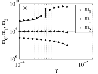
Figure 1: Comparison of simulation and theory. $m_{0}$ the number of families, $m_{1}$ the number of individuals, and $m_{2}$ the second moment. Each point represents a dot on the black line of Fig. 2. See Supplemental Material sup (b) for parameters. Each simulation result is the average over $5$ realizations and $50$ time points separated by $10^{6}$ time steps after steady-state has been established. The lines are the theory and the dots are simulation. Theory and simulation are in perfect fit. $m_{2}$ diverges from point $7$ and on. The theoretic $m_{2}$ in this regime is negative and is not shown here. Empty regions represent values of $0$. See sup (b) for similar results for $N_{1}$.

The theoretical solutions above are valid when:

$$\forall k,N_{k}\geq 0\Longrightarrow\forall j,m_{j}\geq 0.$$ (7)

Imposing these conditions on the steady-state equations (Eqs. 6) leads to:

$$N_{1}\geq 0\Longrightarrow\mu\alpha\geq\gamma$$ (8)

and

$$m_{0}\geq 0\Longrightarrow D=\mu\alpha+\frac{N_{1}}{\bar{N}}(2^{1-\eta}-2+\mu)\geq 0.$$ (9)

The positivity of $m_{1}$ is trivial. The positivity of $m_{2}$ is discussed below. The phase transition defined by both Eq. 8 and Eq. 9 represents the extinction-survival transition.

With no loss of generality, one can set $\alpha\approx 1$, leading to $m_{1}\approx\bar{N}$, for low enough $\gamma$ values. In such a case, the first request resulting from the conditions above is a mutation rate higher than the catastrophe rate, in order to balance the removed families by the creation of new families. The second condition ensures a positive net entry of families to the $k=1$ family-size. If any of these two conditions is breached, the total population collapses.

When one considers the positivity of $m_{2}$, a novel phase transition occurs. Both convergence and positivity of $m_{2}$ are determined by $B$, the pre-factor of $m_{2}$ in $\frac{dm_{2}}{dt}$ (Eq. 3). $B<0$ is the condition for convergence and for positivity. When $B$ is positive the power-law assumption fails and the moment approximations no longer hold. However, the power-law assumption is a good enough approximation to predict the location of the second phase transition, as the comparisons with simulation show. Substituting $m_{1}$ into $B$ we get

$$\gamma>\frac{2\mu}{1-2\mu}\frac{m_{0}}{\bar{N}}$$ (10)

as the condition for both positivity and convergence. In developing this equation we assumed that $\mu<\frac{1}{2}$, as extremely large mutation rates lead to a population collapse Eigen (2002).

Thus, a critical transition emerges, where the family-size variance diverges. This new second phase transition divides the survival phase into “low variance” and “high variance” phases. The diversity of the family-size distribution is governed by $m_{2}$, and when $B$ becomes positive one can expect high diversity in family-size over time and realizations. With the increasing diversity in family-size comes an increasing sensitivity to the collapse of very large families and the resulting fluctuating dynamics. See Supplemental Material sup (b) for simulated $m_{0}$, $m_{1}$, and $m_{2}$ as a function of time. The differences between the dynamics on the two sides of the phase transition are very clear.

The different phases of the model are summarized in the $2$-dimensional phase diagram, Fig. 2, which is a numeric solution of the first two equations of Eqs. 5 and the first three equations of Eqs. 6. It denotes the extinction phase in white, and the line separating it from the survival phase is given by Eq. 8. Eq. 9 is automatically satisfied when Eq. 8 is satisfied. The “high variance” phase defined by Eq. 10 is denoted in blue. The green area is the “low variance” phase, where $B<0$.

One is thus led to the surprising result that as $\gamma$ increases beyond some value the diversity diverges, and the model above fails. Moreover, even in the domain where the model assumptions hold, $m_{2}$ grows with $\gamma$. Thus, in contradiction with current concepts, in the current model, increasing the catastrophe rate actually increases the diversity in time and in the family-size distribution. When $\gamma$ further grows to kill more families than are produced by mutations, the total population collapses, and extinction occurs through a novel phase transition.

Both phase transitions are further illustrated in Fig. 3, where the theoretic solution for the moments and the denominator of $m_{0}$ is given, with fixed $\alpha$, $\gamma$, and $\bar{N}$, but changing $\mu$. For small $\mu$ values the system is extinct. A first phase transition occurs at $\mu\simeq 0.006$, where the system enters the “high variance” phase, and although $m_{0}$ and $m_{1}$ are positive, $m_{2}$ would be negative in the scale free approximation. After $\mu\simeq 0.03$, $m_{2}$, becomes positive too.

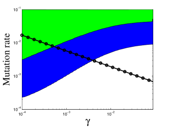
Figure 2: Phase diagram. “Low diversity” phase were $m_{2}$ convergence (green), “high diversity” phase (blue) and extinction phase (white). Results of the theoretic model and solved numerically. Points on the black line were simulated and compared with the numeric solution (see Fig. 1).

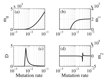
Figure 3: Numeric solution showing both phase transitions. The first phase transition from extinction to survival phase is evident in $D$, the denominator of $m_{0}$. The second phase transition, from “high diversity” to “low diversity”, is evident in $m_{2}$. Here $\gamma=0.01$, $\alpha=1.99$, and $\bar{N}=103890$.

Simulation results confirming the theoretic solution are given in Fig. 1. See Supplemental Material sup (b) for the set of parameters corresponding to each dot in Fig. 1, Fig. 2, and Fig. 4. We chose a set of systems sampling all phases of the model. The first six dots are systems in the “low variance” phase, the next six dots are systems in the “high variance” phase and the remaining ten dots are systems in the extinction phase. The theoretic solution is valid in the “low variance” phase, where a very good agreement with simulations can be observed. In the “high variance” phase, a good agreement with simulations is observed for all moments except $m_{2}$ . The ten extinction phase simulations have very quickly converged with all moments reaching zero, and are not plotted in the graphs.

The increase in $m_{2}$ is also clear in the simulated steady-state family-size distribution. The steady-state size distributions of systems corresponding to the dots on the black line are given in Fig. 4. As $\gamma$ increases, the slope of the power-law decreases, the fraction of large-size families increases, and the maximal family-size increases.

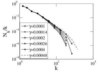
Figure 4: Simulated steady-state family-size distribution, $N_{k}/k$. A line represents a system with parameters defined by dots on the black line of Fig. 2 (see Supplemental Material sup (b) for parameters). As $\gamma$ increases the number of catastrophes increases, the relative number of larger families increases. The maximal family size increases as well.

The intuition behind this mechanism is simple. In the absence of catastrophes, births and deaths must be balanced leading to a Ewens-like family-size distribution Ewens (1972). However, in the presence of catastrophes, the average birth rate of families can be higher than the death rate, with the total population balanced by catastrophes. In such a regime, with an average net growth rate of $\theta$, the family size of a family $k$ is on average as $e^{\theta\tau_{k}}$, where $\tau_{k}$ is the time from the emergence of this family through a mutation to the current time, unless it was destroyed by a catastrophe. For large enough values of $\mu$ the total number of families is arbitrarily large, and the time between catastrophes for a given family increases linearly with the number of families.

In order to validate that such a model does produce the increase in diversity following the increase in catastrophes rate, we simulated a model where in each time step $\Delta t$, the following reactions occur:

• $\gamma m_{0}$ out of $m_{0}$ families are destroyed using a random choice with a Binomial distribution.

• $\mu m_{1}$ families are produced randomly with a Poisson distribution.

• Each family grows by a factor of $exp\big{[}(\alpha-\mu-m_{1}/N)\Delta t\big{]}$.

Here, as in the original model, $\alpha$ is the birth rate, $N$ is some arbitrary large number, $\mu$ is the mutation rate, and $\gamma$ is the catastrophes rate. Indeed, this simulation reproduces the relation above (see Supplemental Material sup (c) for family-size distribution of this model), with the clear phase transition to very high $m_{2}$ values. Moreover, the catastrophe size increases with $\gamma$. When $\gamma$ becomes larger than $\mu$, the total population collapses as in the original model.

While we have here studied a single specific model, the same results hold in different domains, with different dynamics (see Supplemental Material sup (d, e) for details of other models where the same results hold). The main element driving these results is that, in equilibrium, the total population is governed by a balance between family growth and decay. However, while the death term affects all families equally, the catastrophe term affects a random subset of families. Since a part of the death term is balanced by the catastrophes, the remaining total death term is lower than the total birth rate. Thus, for families not dying by catastrophes, the net difference between growth and death is positive, leading to an exponential growth, until a catastrophe occurs. Therefore, increasing the catastrophe rate increases the net growth rate and decreases the time between catastrophe events. Such a balance can be observed in many scenarios, such as the growth of stock values in stock markets, family growth in highly fluctuating environments, or the dynamics of network, where vertices can accumulate edges, until a vertex deletion event happens.

While large jumps in single families (e.g. Lévy flights) have been extensively studied Mandelbrot (1982), these jumps are assumed to be averaged and not to induce very large changes in large ensembles. This is in clear contrast with large-scale fluctuations observed, among others, in the total market value of stock markets. The influence of frequent catastrophes may be one element explaining these fluctuations. An important element obviously missing from the current description is the interaction between families and the possibility of cascades from one collapsing population to the other. We now plan to study whether the mechanisms described here apply when interactions are taken into account.

in 1,…,8 See pages \x of SuppMat34.pdf

References

- Weng et al. (2012) E. Weng, Y. Luo, W. Wang, H. Wang, D. J. Hayes, A. D. McGuire, A. Hastings, and D. S. Schimel, Journal of Geophysical Research: Biogeosciences 117 (2012).
- Leite et al. (2012) M. C. A. Leite, N. P. Petrov, and E. Weng, Nonlinear Analysis: Real World Applications 13, 497 (2012).
- Mawby et al. (1989) W. Mawby, F. Hain, and C. Doggett, Forest Science 35, 1075 (1989).
- Turcotte (1999) D. L. Turcotte, Reports on Progress in Physics 62, 1377 (1999).
- Chen-Charpentier and Leite (2014) B. Chen-Charpentier and M. Leite, Ecological Modelling 286, 26 (2014).
- Wilcox and Elderd (2003) C. Wilcox and B. Elderd, Journal of Applied Ecology 40, 859 (2003).
- Petraitis (2013) P. Petraitis, Multiple stable states in natural ecosystems (OUP Oxford, 2013).
- Scheffer et al. (2001) M. Scheffer, S. Carpenter, J. A. Foley, C. Folke, and B. Walker, Nature 413, 591 (2001).
- Ives and Cardinale (2004) A. R. Ives and B. J. Cardinale, Nature 429, 174 (2004).
- Hart and Avilés (2014) E. M. Hart and L. Avilés, PloS one 9, e110049 (2014).
- Tuljapurkar (2013) S. Tuljapurkar, Population dynamics in variable environments, Vol. 85 (Springer Science & Business Media, 2013).
- Froot and O’Connell (2008) K. A. Froot and P. G. O’Connell, Journal of Banking & Finance 32, 69 (2008).
- He and Krishnamurthy (2012) Z. He and A. Krishnamurthy, The Review of Economic Studies 79, 735 (2012).
- Enjolras and Kast (2012) G. Enjolras and R. Kast, Agricultural Finance Review 72, 156 (2012).
- Nowak and Romaniuk (2013) P. Nowak and M. Romaniuk, Insurance: Mathematics and Economics 52, 18 (2013).
- Falco et al. (2014) S. D. Falco, F. Adinolfi, M. Bozzola, and F. Capitanio, Journal of Agricultural Economics 65, 485 (2014).
- Pruessner (2012) G. Pruessner, Self-organised criticality: theory, models and characterisation (Cambridge University Press, 2012).
- Malamud et al. (1998) B. D. Malamud, G. Morein, and D. L. Turcotte, Science 281, 1840 (1998).
- Drossel and Schwabl (1992) B. Drossel and F. Schwabl, Physical Review Letters 69, 1629 (1992).
- Bak et al. (1988) P. Bak, C. Tang, and K. Wiesenfeld, Physical Review A 38, 364 (1988).
- Kadanoff et al. (1989) L. P. Kadanoff, S. R. Nagel, L. Wu, and S.-m. Zhou, Physical Review A 39, 6524 (1989).
- Yoder et al. (2011) M. R. Yoder, D. L. Turcotte, and J. B. Rundle, Physical Review E 83, 046118 (2011).
- Clar et al. (1994) S. Clar, B. Drossel, and F. Schwabl, Physical Review E 50, 1009 (1994).
- Clar et al. (1996) S. Clar, B. Drossel, and F. Schwabl, Journal of Physics: Condensed Matter 8, 6803 (1996).
- Noël et al. (2013) P.-A. Noël, C. D. Brummitt, and R. M. D’Souza, Physical Review Letters 111, 078701 (2013).
- Stanley et al. (2002) H. E. Stanley, L. A. N. Amaral, P. Gopikrishnan, V. Plerou, and B. Rosenow, in Empirical Science of Financial Fluctuations (Springer, 2002) pp. 3–11.
- Fu et al. (2005) D. Fu, F. Pammolli, S. V. Buldyrev, M. Riccaboni, K. Matia, K. Yamasaki, and H. E. Stanley, Proceedings of the National Academy of Sciences of the United States of America 102, 18801 (2005).
- Huynen and Van Nimwegen (1998) M. A. Huynen and E. Van Nimwegen, Molecular Biology and Evolution 15, 583 (1998).
- Koonin et al. (2002) E. V. Koonin, Y. I. Wolf, and G. P. Karev, Nature 420, 218 (2002).
- Qian et al. (2001) J. Qian, N. M. Luscombe, and M. Gerstein, Journal of Molecular Biology 313, 673 (2001).
- Luscombe et al. (2002) N. M. Luscombe, J. Qian, Z. Zhang, T. Johnson, and M. Gerstein, Genome Biology 3, Research0040 (2002).
- Wójtowicz and Tiuryn (2007) D. Wójtowicz and J. Tiuryn, Journal of Computational Biology 14, 479 (2007).
- Reed and Hughes (2004) W. J. Reed and B. D. Hughes, Mathematical Biosciences 189, 97 (2004).
- Csűrös and Miklós (2006) M. Csűrös and I. Miklós, in Annual International Conference on Research in Computational Molecular Biology (Springer, 2006) pp. 206–220.
- Hahn et al. (2005) M. W. Hahn, T. De Bie, J. E. Stajich, C. Nguyen, and N. Cristianini, Genome Research 15, 1153 (2005).
- Gabetta and Regazzini (2010) E. Gabetta and E. Regazzini, Mathematical Models and Methods in Applied Sciences 20, 1005 (2010).
- sup (a) (a), supplementary Material I Main Model Equations Derivation.
- sup (b) (b), supplementary Material IV Supporting Material for Main Model.
- Eigen (2002) M. Eigen, Proceedings of the National Academy of Sciences 99, 13374 (2002).
- Ewens (1972) W. J. Ewens, Theoretical Population Biology 3, 87 (1972).
- sup (c) (c), supplementary Material V Exponential Model.
- sup (d) (d), supplementary Material II Spatial Epidemics Model.
- sup (e) (e), supplementary Material III Network Model.
- Mandelbrot (1982) B. B. Mandelbrot, The Fractal Geometry of Nature (New York: W. H. Freeman., 1982).