Differentiable Submodular Maximization

Abstract

We consider learning of submodular functions from data. These functions are important in machine learning and have a wide range of applications, e.g. data summarization, feature selection and active learning. Despite their combinatorial nature, submodular functions can be maximized approximately with strong theoretical guarantees in polynomial time. Typically, learning the submodular function and optimization of that function are treated separately, i.e. the function is first learned using a proxy objective and subsequently maximized. In contrast, we show how to perform learning and optimization jointly. By interpreting the output of greedy maximization algorithms as distributions over sequences of items and smoothening these distributions, we obtain a differentiable objective. In this way, we can differentiate through the maximization algorithms and optimize the model to work well with the optimization algorithm. We theoretically characterize the error made by our approach, yielding insights into the tradeoff of smoothness and accuracy. We demonstrate the effectiveness of our approach for jointly learning and optimizing on synthetic maximum cut data, and on real world applications such as product recommendation and image collection summarization.

1 Introduction

Many important applications require the prediction of set-valued outputs, e.g. product recommendation in which the output corresponds to a set of items that should be recommended to a user, object detection in images in which the output is a set of bounding boxes Felzenszwalb et al. (2010), or extractive summarization in which the output is a set of input objects (sentences in text summarization Lin and Bilmes (2010), images in image collection summarization Tschiatschek et al. (2014), short scenes in video summarization Zhang et al. (2016)). This problem is particularly challenging as the size of the output space (i.e. the number of possible subsets of some ground set, e.g. the set of all possible bounding boxes) increases exponentially with the size of the ground set.

The problem of learning to predict sets is most commonly approached by either specifying suitable set functions by hand or by first learning the set functions for the task at hand from data and then performing inference using the learned set function. To enjoy strong theoretical guarantees for inference via maximization, we are interested in using set functions that are submodular. The submodular set functions are fitted to the given training data (we consider the supervised case in which the training data contains the sets we wish to predict) using, for example, large margin methods Lin and Bilmes (2012); Tschiatschek et al. (2014), maximum likelihood estimation Gillenwater et al. (2014); Tschiatschek et al. (2016) or by minimizing some kind of set-valued loss function Dolhansky and Bilmes (2016). Finally, for inference, some variant of greedy algorithm is used for maximizing the learned set function.

This approach suffers from the problem that training and testing are performed differently which can lead to degraded performance. Furthermore, this approach circumvents end-to-end training of the considered functions. However, end-to-end training is desirable as it often leads to significant performance improvements as demonstrated on various domains recently Ren et al. (2015); Bahdanau et al. (2014).

We resolve this problem by proposing two differentiable algorithms for maximizing non-negative submodular set functions with cardinality constraints and without constraints. These algorithms can easily be integrated into existing deep learning architectures. The algorithms define a likelihood over sets and are used for both training and testing. This enables end-to-end training of functions for predicting sets. Our algorithms are derived from the standard greedy algorithm Nemhauser et al. (1978) and the double greedy algorithm Buchbinder et al. (2015) which was originally proposed for maximizing positive non-monotone submodular functions and provides a $\tfrac{1}{2}$ approximation guarantee. Interestingly, our algorithm for unconstrained maximization also provides approximation guarantees of the form $f(X_{G})\geq\tfrac{1}{2}f(\textnormal{OPT})-\epsilon(t)$, where $\epsilon(t)$ is a function of the parameter $t$ parameterizing our algorithm, OPT is an optimal solution and $X_{G}$ is the output of our algorithm.

Our main contributions are:

1. We develop differentiable algorithms for end-to-end training of deep networks with set-valued outputs.

2. We theoretically characterize the additional errors imposed by smoothing used in the derivation of our algorithm for unconstrained maximization.

3. We demonstrate the excellent end-to-end learning performance of our approach on several challenging applications, including product recommendation and image collection summarization.

2 Notation & Problem Setting

Notation. Let $\mathcal{V}=\{e_{1},e_{2},\ldots\}$ be a ground set of items. We want to perform subset selection from $\mathcal{V}$. In some parts of the paper we consider $\mathcal{V}$ to be fixed while in others $\mathcal{V}$ depends on the context. Note that we assume an arbitrary but fixed enumeration of the items in $\mathcal{V}$. Furthermore, let $f\colon 2^{\mathcal{V}}\rightarrow\mathbb{R}$ be a set function assigning a real-valued scalar to every set $S\subseteq\mathcal{V}$. The function $f$ is submodular iff $f(A\cup\{e\})-f(A)\geq f(B\cup\{e\})-f(B)$ for all $e\in\mathcal{V},A\subseteq B\subseteq\mathcal{V}\setminus\{e\}$. The function $f$ is monotone if $f(A)\leq f(B)$ for all $A\subseteq B$ and non-monotone otherwise. We denote the gain of adding an item $e\in\mathcal{V}$ to a set of items $S$ by $\Delta^{+}_{f}(e\mid S)=f(S\cup\{e\})-f(S)$ and the gain of removing the item $e\in S\subseteq\mathcal{V}$ from a set $S$ as $\Delta^{-}_{f}(e\mid S)=f(S\setminus\{e\})-f(S)$. We will omit the subscript $f$ whenever the function $f$ is clear from the context. For notational convenience we write $S+e$ instead of $S\cup\{e\}$ and $S-e$ instead of $S\setminus\{e\}$.

Problem setting. We consider the problem of learning an unknown submodular function $f(S\mid\mathcal{V})$ from training data. The training data is given in the form of a collection of maximizers $\mathcal{X}$ (or approximate maximizers) of $f(S\mid\mathcal{V})$ for different ground sets $\mathcal{V}$, i.e. $\mathcal{X}=\{(\mathcal{V}_{1},X_{1}),\ldots,(\mathcal{V}_{M},X_{M})\}$. We assume that the ground set is not only an abstract set of elements but that for every element in the ground set we have additional information, e.g. an associated vector of features. For instance, in the case of image collection summarization, the ground set $\mathcal{V}_{i}$ corresponds to the images (each element of $\mathcal{V}_{i}$ comes in form of an actual image in form of pixel values) in an image collection and the set $X_{i}$ is a human generated summary for that collection. Note that the training data can contain multiple samples for the same ground set, e.g. in image collection summarization there can be multiple human generated summaries for some particular image collection. The (approximate) maximizers in $\mathcal{X}$ either maximize $f(S\mid\mathcal{V})$ unconstrainedly, i.e. $\forall(\mathcal{V},X)\in\mathcal{X}$ it holds that $f(X\mid\mathcal{V})\approx\max_{S\in\mathcal{V}}f(S)$ or cardinality constrainedly, i.e. $f(X)\approx\max_{S\in\mathcal{V},|S|\leq k}f(S\mid\mathcal{V})$ for some cardinality constraint $k$. Given an algorithm ApproxMax that can approximately maximize a submodular function with or without cardinality constraints, our goal is to learn a set function $h_{\theta}(S\mid\mathcal{V})$ parameterized by $\theta$ such that if it is maximized with ApproxMax, the returned solutions approximately maximize $f(S\mid\mathcal{V})$. For the image collection summarization application, maximizing $h_{\theta}(S\mid\mathcal{V})$ with ApproxMax should generalize to new unseen ground sets $\mathcal{V}$, i.e. yield subsets of images that summarize an unseen image collection well, respectively. For other applications, e.g. the product recommendation application, maximizing the function $h_{\theta}$ with ApproxMax should yield good solutions conditioned on the selection of a subset of items (see the experimental section for details).

Our approach—learning to greedily maximize. We develop two probabilistic approximate maximization algorithms ApproxMax that take a function $h_{\theta}(\cdot|\mathcal{V})$ parameterized by $\theta$ as input and output approximate maximizers of $h_{\theta}(\cdot|\mathcal{V})$. These algorithms are based on the standard greedy algorithm and the double greedy algorithm and presented in detail in the next sections. Because of the probabilistic nature of the algorithms, they induce a distribution over sets $S\subseteq\mathcal{V}$ as $P_{\textsc{ApproxMax}}(S;h_{\theta}(\cdot|\mathcal{V}))=P(\textsc{ApproxMax}(h_{\theta}(\cdot|\mathcal{V}))=S)$. We can thus equivalently view these probabilistic algorithms ApproxMax as distributions over sets. To learn the parameters of the function $h_{\theta}$, we can thus maximize the likelihood $\mathcal{X}$ under the induced distribution, i.e. we aim to find

$$\theta^{*}=\arg\max_{\theta}\sum_{(\mathcal{V},X)\in\mathcal{X}}\log P_{\textsc{ApproxMax}}(X;h_{\theta}(\cdot|\mathcal{V})).$$ (1)

The parameters $\theta^{*}$ according to the above equation intimately connect the function $h_{\theta^{*}}$, the algorithm ApproxMax, and the function $f$, i.e. ApproxMax computes approximate maximizers of $f$ when applied to $h_{\theta^{*}}$. By ensuring that our developed approximate maximization algorithms have differentiable likelihoods, we can maximize our objective in (1) using gradient based optimization techniques. This enables the easy integration of our algorithms into deep learning architectures which are commonly optimized using stochastic gradient descent techniques.

3 Differentiable Unconstrained Maximization

In this section we present our probabilistic algorithm PD²Greedy for differentiable unconstrained maximization of non-negative submodular set functions. The algorithm is derived from the double greedy algorithm Buchbinder et al. (2015) and presented in Algorithm 1.

The algorithm works by iterating through the items in $\mathcal{V}$ in a fixed order. In every iteration it computes the gain $a_{i}$ for adding the $i$th item to the set $X_{i-1}$ and the gain $b_{i}$ for removing the $i$th item from the set $Y_{i-1}$. It then compares these two gains and makes a probabilistic decision based on that comparison.

Algorithm 1 PD²Greedy: Probabilistic diff. double-greedy

Function $h_{\theta}\colon\mathcal{V}\rightarrow\mathbb{R}_{\geq 0}$

$X_{0}\leftarrow\emptyset$

$Y_{0}\leftarrow\mathcal{V}$

for $i=1,\ldots,|\mathcal{V}|$ do

     $a_{i}=h_{\theta}(X_{i-1}+e_{i})-h_{\theta}(X_{i-1})$ $\triangleright$ $\hat{=}\Delta^{+}(e_{i}\mid X_{i-1})$

     $b_{i}=h_{\theta}(Y_{i-1}-e_{i})-h_{\theta}(Y_{i-1})$ $\triangleright$ $\hat{=}\Delta^{-}(e_{i}\mid Y_{i-1})$

     if $g(a_{i},b_{i})\geq\mathcal{U}$ then $\triangleright$ $\mathcal{U}$ is uniform dist. on $[0,1]$

         $X_{i}=X_{i-1}\cup\{e_{i}\}$

     else

         $Y_{i}=Y_{i-1}\setminus\{e_{i}\}$

     end if

end for

return Approximate maximizer $X_{|\mathcal{V}|}$

The deterministic and randomized version of the double greedy algorithm as presented in  Buchbinder et al. (2015) can be obtained from Algorithm 1 by specific choices of the function $g(a_{i},b_{i})$. In particular, setting $g(a,b)=g_{1}(a,b)\coloneqq\mathbf{1}_{a>b}$, where $\mathbf{1}$ is the indicator function, results in the deterministic double greedy algorithm with a $\tfrac{1}{3}$ approximation guarantee for maximizing positive non-monotone submodular functions. Setting $g(a,b)=g_{2}(a,b)\coloneqq\tfrac{[a]_{+}}{[a]_{+}+[b]_{+}}$, where $[x]_{+}=\max\{0,x\}$, results in the randomized double greedy algorithm with a $\tfrac{1}{2}$ approximation guarantee for maximization in expectation.

Note that the algorithm, independent of the particular choice of $g(a_{i},b_{i})$, induces a distribution over subsets of $\mathcal{V}$. To specify this distribution, let $x$ be a binary vector representing the set $X$ in form of a one-hot encoding for the assumed fixed ordering $e_{1},e_{2},\ldots$ of the elements in the ground set. Then, the distribution is

$$P_{\textsc{PD\textsuperscript{2}Greedy}}(X)=\prod_{i=1}^{|\mathcal{V}|} g(a_{i},b_{i})^{x_{i}}(1-g(a_{i},b_{i}))^{1-x_{i}},$$ (2)

where $a_{i}=\Delta^{+}(e_{i}\mid\{e_{j}\mid j<i,x_{j}=1\})$ and $b_{i}=\Delta^{-}(e_{i}\mid\{e_{j}\in\mathcal{V}\mid j\geq i\textnormal{ or }x_{j}=1\})$. Obviously, this distribution depends on the order of the items which we assumed to be fixed. In practice, this order influences the maximization performance as substantiated by an example shortly.

While Equation (2) defines a distribution over sets it is hard to optimize for $g=g_{1}$ and $g=g_{2}$ because of the non-smoothness of these functions. Thus we propose the following two natural smooth alternatives for the function g:

• $g(a,b)=g_{3}(a,b;t)\coloneqq\mu(a,b;t)$ is an approximation to the deterministic double greedy algorithm which becomes exact as $t\rightarrow 0$ where $\mu(a,b;t)=\tfrac{1}{1+\exp(-(a-b)/t)}$

• $g(a,b)=g_{4}(a,b;t)\coloneqq\tfrac{a^{\prime}}{a^{\prime}+b^{\prime}}$, where $a^{\prime}=t\log(1+\exp(\tfrac{a}{t}))$ and $b^{\prime}=t\log(1+\exp(\tfrac{b}{t}))$ is an approximation to the randomized double greedy algorithm which becomes exact as $t\rightarrow 0$.

Interestingly, choosing one of these smooth alternatives for the function $g(a,b)$ still results in an algorithm with approximation guarantees to the true optimum as substantiated in the following theorems.

Theorem 1.

Let $\epsilon>0$ and $g(a,b)=g_{4}(a,b;t)$. For $t<\tfrac{2\epsilon}{|\mathcal{V}|\log(2)}$, the output $X_{|\mathcal{V}|}$ of Algorithm 1 satisfies $f(X_{|\mathcal{V}|})\geq\tfrac{1}{2}f(\textnormal{OPT})-\epsilon$ in expectation, where $f(\textnormal{OPT})$ is an optimal solution.

Similarly, for the approximation to the deterministic algorithm we have the following theorem.

Theorem 2.

Let $\epsilon>0$ and $g(a,b)=g_{3}(a,b;t)$. For $t<\tfrac{3\epsilon}{|\mathcal{V}|W(1/e)}$, the output $X_{|\mathcal{V}|}$ of Algorithm 1 satisfies $f(X_{|\mathcal{V}|})\geq\tfrac{1}{3}f(\textnormal{OPT})-\epsilon$ in expectation, where $f(\textnormal{OPT})$ is an optimal solution.

The full proofs are omitted due to space constraints and available in the extended version of this paper Tschiatschek et al. (2018). The idea of the proofs of Theorems 1 and 2 is as follows: Instead of using $g_{1}$ and $g_{2}$ in Algorithm 1, we use $g_{3}$ and $g_{4}$, respectively. Note that as $t\rightarrow 0$, the approximation of $g_{1}$ by $g_{3}$ becomes exact (the same holds for the approximation of $g_{2}$ by $g_{4}$). For nonzero $t$, the considered approximations change the probabilities of selecting each item $e_{i}$ during the execution of Algorithm 1 and introduce an (additive) error compared to executing Algorithm 1 with $g_{1}$ and $g_{2}$, respectively. We can guarantee that this additive error is below any desired error $\epsilon/|\mathcal{V}|$ by choosing $t$ small enough. As the algorithm iterates over all items, the total error is then bounded by $\epsilon$.

Theorems 1 and 2 characterize a tradeoff between accuracy of the algorithm and smoothness of the approximation. High accuracy (small $\epsilon$) requires low smoothness (small $t$) and vice versa.

Speeding up computations. Naively computing the likelihood in Equation (2) requires $4|\mathcal{V}|$ function evaluations. By keeping track of the function values $f(X_{i})$ and $f(Y_{i})$ this can immediately be reduced to $2|\mathcal{V}|$ function evaluations. However, for large $|\mathcal{V}|$ this may still be prohibitive. Fortunately, many submodular functions allow for fast computation of all $a_{i}$ and $b_{i}$ values needed for evaluating (2). For example, for the modular function $f(S)=\sum_{e\in S}s_{e}$, where $s_{e}\in\mathbb{R}$, the gains for computing $\textsc{PD\textsuperscript{2}Greedy}(X)$ are $a_{i}=s_{e_{i}}$ and $b_{i}=-s_{e_{i}}$. Another example is the facility location function $f(S)=\max_{e\in S}w_{e}$, where $w_{e}\in\mathbb{R}_{\geq 0}$. In that case, $a_{i}$ can be iteratively computed as $a_{i}=\max\{c_{i-1},w_{e_{i}}\}$ where $c_{i}=\max\{c_{i-1},w_{e_{i}}\}$ if $e_{i}\in X$ and $c_{i}=c_{i-1}$ otherwise (setting $c_{0}=-\infty$ for initialization).

Non non-negative functions. Some of the functions we are learning in the experiments in Section 5 are not guaranteed to be non-negative over their whole domain. This seems problematic because the above guarantees only hold for non-negative functions. Note that any set function $\hat{f}(S)$ can be transformed into a non-negative set function $f(S)$ by defining $f(S)=\hat{f}(S)-\min_{S^{\prime}\in\mathcal{V}}\hat{f}(S^{\prime})$. This transformation does not affect the gains $a_{i}$ and $b_{i}$ computed in Algorithm 1, however it changes the values of the maxima.

Ordering of the items. The ordering of the items in the ground set influences the induced distributions over sets. Furthermore it can have a significant impact on the achieved maximization performance, although the theoretical guarantees are independent of this ordering. To see this, consider the following toy example and PD²Greedy with $g=g_{1}$: Let $\mathcal{V}=\{e_{1},e_{2}\}$, $w_{e_{1}}=2,w_{e_{2}}=1$ and $f(S)=2+\max_{i\in S}w_{i}-|S|^{2}$. This function is non-negative submodular with $f(\emptyset)=2,f(\{e_{1}\})=3,f(\{e_{2}\})=2,f(\mathcal{V})=0$. If the items in PD²Greedy were considered in the the order $(e_{1},e_{2})$, the algorithm would return $\{e_{2}\}$ with a function value of $2$ while it would return $\{e_{1}\}$ with a function value of $3$ if the items were considered in the reversed order $(e_{2},e_{1})$. Note that similar observations hold for all choices of $g$.

Connection to probabilistic submodular models. Algorithm PD²Greedy defines a distribution over sets and there is an interesting connection to probabilistic submodular models  Djolonga and Krause (2014) Specifically, for the case that $f(S)$ is a modular function, $g=g_{3}$ and $t=2$, the induced distribution of PD²Greedy corresponds to that of a log-modular distribution, i.e. items $e_{i}$ are contained in the output of PD²Greedy with probability $\sigma(f(\{e_{i}\})$.

4 Diff. Cardinality Constrained Maximization

In this section we present our algorithm for differentiable cardinality constrained maximization of submodular functions. We assume that the cardinality constraint is $k$, i.e. $\forall_{(\mathcal{V},X)\in\mathcal{X}}\colon f(X)\approx\max_{S\subseteq\mathcal{V},|S|=k}f(S)$.

Our algorithm PGreedy is presented in Algorithm 2. The algorithm iteratively builds up a solution of $k$ elements by adding one element in every iteration, starting from the empty set. The item added to the interim solution in iteration $i$ is selected randomly from all not yet selected items $\mathcal{V}\setminus X_{i-1}$, where the probability $p_{e\mid X_{i-1}}$ of selecting item $e$ depends on the gain of adding $e$ to $X_{i-1}$. The selection probabilities are controlled by the temperature $t$. Assuming no ties, for $t\rightarrow 0$, PGreedy is equivalent to the standard greedy algorithm, deterministically selecting the element with highest marginal gain in every iteration.

The algorithm naturally induces a differentiable distribution over sequences of items $\sigma=(e_{1},\ldots,e_{k})$ of length $k$ at temperature $t$ such that

$$P(\sigma)=\prod_{i=1}^{k}\frac{\exp(\tfrac{1}{t}\Delta^{+}_{h_{\theta}}(\sigma_{i}\mid X_{i-1}))}{\sum_{e^{\prime}\in\mathcal{V}\setminus X_{i-1}}\exp(\tfrac{1}{t}\Delta^{+}_{h_{\theta}}(e^{\prime}\mid X_{i-1}))},$$ (3)

where $X_{i-1}=\{\sigma_{1},\ldots,\sigma_{i-1}\}$. From this distribution, we derive the probability of a set $S$ by summing over all sequences $\sigma$ of items consistent with $S$, i.e.

$$P(S)=\sum_{\sigma\in\Sigma(S)}P(\sigma),$$ (4)

where $\Sigma(S)$ is the set of permutations of the elements in $S$.

Algorithm 2 PGreedy: Probabilistic differentiable greedy

Function $h_{\theta}\colon\mathcal{V}\rightarrow\mathbb{R}_{\geq 0}$, cardinality constraint $k$

$X_{0}\leftarrow\emptyset$

for $i=1,\ldots,k$ do

     $\mathcal{C}\leftarrow\mathcal{V}\setminus X_{i-1}$

     $\forall e\in\mathcal{C}\colon p_{e\mid X_{i-1}}\leftarrow\frac{\exp\big{(}\tfrac{1}{t}\Delta^{+}_{h_{\theta}}(e\mid X_{i-1})\big{)}}{\sum_{e^{\prime}\in\mathcal{C}}\exp\big{(}\tfrac{1}{t}\Delta^{+}_{h_{\theta}}(e^{\prime}\mid X_{i-1})\big{)}}$

     $e^{*}\leftarrow$ sample $e$ from $\mathcal{C}$ with probability $p_{e\mid X_{i-1}}$

     $X_{i}=X_{i-1}\cup\{e^{*}\}$

end for

return Approximate maximizer $X_{k}$

As already briefly mentioned, the probability of a set $S$ depend on the temperature $t$. For $t=0$ there is at most one permutation $\sigma$ of the items in $S$ for which $P(\sigma)$ is non-zero (assuming that there are no ties). In contrast, for $t\rightarrow\infty$, $P(S\mid\sigma)$ is constant for all permutations. Similarly to the case of PD²Greedy, the choice of the temperature $t$ allows to trade-off accuracy (the standard greedy algorithm has a $(1-1/e)$ approximation guarantee for cardinality constraint maximization of non-negative monotone functions) and smoothness. The higher the temperature, the smoother is the induced distribution but the further are the made decisions from the greedy choice.

Learning with PGreedy. Given training data $\mathcal{X}$, we can optimize the parameters of the function $h_{\theta}$ by maximizing the likelihood of $\mathcal{X}$ under the distribution (4). However, for large $k$ computing the summation over $\sigma\in\Sigma(S)$ is infeasible. We propose two approximations for this case:

• If $t$ is small, $P(S)$ can be accurately approximated by $P(\sigma^{*}(S))$ where $\sigma^{*}(S)=\arg\max_{\sigma\in\Sigma(S)}P(\sigma)$. However, to find $\sigma^{*}$ we would still have to search over all possible permutations of $S$. Hence, we propose to approximate $\sigma^{*}(S)$ by the permutation $\sigma^{G}(S)$ induced by the greedy order of the elements in $S$.

• Assuming there is no clear preference on the order of the items in $S$, i.e. $P(\sigma_{i})\approx P(\sigma_{j})$ for all $\sigma_{i},\sigma_{j}\in\Sigma(S)$, we can approximate $P(S)$ as $P(S)\approx k!P(\sigma^{R})$, where $\sigma^{R}$ is a random permutation of the items in $S$.

Testing. If $k$ is known at test time, e.g. we aim to compute a summary of fixed size in the image collection summarization application, we can simply execute the standard greedy algorithm using the learned function $h_{\theta}$. This returns an approximate MAP solution for $P(S)$. However, we can also generate approximate maximizers of $h_{\theta}$ by invoking Algorithm 2. This can be beneficial in cases where we want to propose several candidate summaries to a user to choose from.

5 Experiments

5.1 Maximum Cut

Let $G(\mathcal{V},E,w)$ be a weighted undirected graph, where $\mathcal{V}$ denotes the set of vertices, $E$ is the set of edges and $w$ denotes the set of non-negative edge weights $w_{ij}$, $\forall(i,j)\in E$. The maximum cut problem is to find a subset of nodes $S$ such that the cut value $f(S)=\sum_{i\in S}\sum_{j\in V\setminus S}w_{ij}$ is maximized. The cut function $f(S)$ is non-negative, non-monotone and submodular and has, for instance, been used in semi-supervised learning Wang et al. (2013).

We generate synthetic data for our maximum cut experiment as follows. We first generate $n$ vectors $x_{1},\ldots,x_{n}\in\mathbb{R}^{d}$ by sampling their components uniformly from $[0,1]$ and arrange them in a $n\times d$ matrix $\mathbf{X}$. Using a projection matrix $\mathbf{P}$ of size $k\times d$, we project each $x_{i}$ to the lower dimensional space $\mathbb{R}^{k}$. The weights of the graph $w$ are defined using an RBF kernel $\mathbf{K}$ on these projected vectors. For the resulting graph instance $G(\mathcal{V},E,w)$ we compute the maximum cut $S^{*}\subseteq V$ using IP (Integer Programming) formulation in Gurobi Gurobi Optimization (2016).

We sample $\mathbf{X}_{1},\mathbf{X}_{2},\ldots,\mathbf{X}_{m}$ as described above and, using the same projection matrix $\mathbf{P}$ and RBF kernel $\mathbf{K}$, we generate weights $w^{i}$ for the $m$ graphs and find the maximum cut $S^{*}_{i}$ by IP for each of these graphs. From this data we compose our training set as $\mathcal{X}=\{(\mathbf{X}_{1},S^{*}_{1}),\ldots,(\mathbf{X}_{m},S^{*}_{m})\}$. The test set is composed using the same strategy.

In this experiment, our aim is to learn a projection matrix $\hat{\mathbf{P}}$ such that PD²Greedy, if executed on the graph induced by the points $\hat{\mathbf{P}}\mathbf{X}_{i}$, returns $S^{*}_{i}$. Note that our goal is not necessarily to recover the original projection matrix $\mathbf{P}$—we are only interested in a projection matrix that allows us to find high value cuts through PD²Greedy. For each element of the test set, we compute the corresponding graph using $\hat{\mathbf{P}}$ and find the maximum cut using PD²Greedy and call the set as $S^{l}_{DG}$. We compute the corresponding graph using $\mathbf{P}$ and a random projection matrix, which acts as a baseline, $\mathbf{P}_{r}$ and find the maxcut using PD²Greedy; we refer to these cuts as $S^{o}_{DG}$ and $S^{r}_{DG}$ respectively. When the cut value is calculated using IP, we refer to it as $S^{o}_{IP}$. We compare the ratio of the each cut value calculated by PD²Greedy to the cut value calculated by IP.

Results are shown in Table 1. We observe that cuts computed with PD²Greedy using the learned projection matrix outperform cuts computed via random projection matrices and the original projection matrix. The number of nodes in the graph is $n$, the temperature of the PD²Greedy is $t$ and $0.3$ is used as a bandwidth parameter for the RBF kernel. The original points $x_{i}$ are in $\mathbb{R}^{10}$ and they are projected into $\mathbb{R}^{5}$ using the first 5 coordinates. Our training and test set consists of $800$ and $200$ elements, respectively. During training and testing, we used $g_{4}(a,b;t)$ to define the likelihood of sets as in Equation (2). For optimization, we used Adam Kingma and Ba (2015) with batch size of $16$ and initial learning rate $0.02$. In every case, we benefit from learning the projection matrix.

Parameters	$S^{l}_{DG}$	$S^{o}_{DG}$	$S^{r}_{DG}$
n=20, t=$2^{-3}$	0.88 $\pm$ 0.008	0.86 $\pm$ 0.010	0.64 $\pm$ 0.012
n=20, t=$2^{-2}$	0.84 $\pm$ 0.007	0.80 $\pm$ 0.009	0.62 $\pm$ 0.012
n=20, t=$2^{-1}$	0.79 $\pm$ 0.006	0.74 $\pm$ 0.007	0.60 $\pm$ 0.008
n=20, t=1	0.74 $\pm$ 0.006	0.69 $\pm$ 0.007	0.60 $\pm$ 0.008

Table 1: Performance of different cuts for varying temperature $t$ in PD²Greedy. The cuts $S^{l}_{DG}$ computed from PD²Greedy using the learned projection matrix outperforms cuts computed via random projection matrices and the original projection matrix. This indicates that the learned projection matrix is optimized to accommodate our probabilistic greedy algorithm.

5.2 On the Relation Between Learning and Temperature

In this section we experimentally investigate the relation between temperature and the difficulty of parameter learning, providing rather informal but intuitive explanations for the results of our paper. Our findings are based on the experimental setting of Section 5.1. Figure 1 shows training log-likelihoods for different temperatures over training epochs on synthetic data.

For low temperatures $t$ ($t=2^{-5}$ and $t=2^{-4}$), we observe that the log-likelihood quickly converges to a (relatively) low log-likelihood level. For these low temperatures, the link function $g_{4}$ is relatively close to $g_{2}$, the standard link function of the randomized double greedy algorithm. However, as $g_{4}$ becomes less smooth with decreasing $t$, the corresponding gradients become non-informative and learning is more difficult.

For high temperatures $t$ ($t=2^{2}$ and $t=2^{3}$), we also observe that the log-likelihoods converge to a (relatively) low log-likelihood level. For these high temperatures, $g_{4}$ is very smooth but far from $g_{2}$. With increasing temperature, the probability distribution over sets becomes more uniform and non-informative. Because of the smoothness of $g_{4}$, the optimization becomes easier but it converges to a distribution that does not put much probability mass on the approximate maximizers that we are interested in.

For medium temperatures $t$ ($t=2^{-3}$ and $t=2^{-2}$) we observe the highest log-likelihoods. This is also reflected in the test set performance in our other synthetic experiments, cf. Table 1. For these medium temperatures, $g_{4}$ is smooth enough to provide informative gradients and close enough to the original link function $g_{2}$ to preserve the correct probability distribution over sets.

To summarize, there is a trade-off between temperature and difficulty of parameter learning. Although Theorems 1 and 2 suggest that using a temperatures $t$ as small as possible should lead to the smallest additive error compared to the corresponding variants of the double greedy algorithm, using low temperatures $t$ can make training difficult. Using high temperatures $t$ also results in bad log-likelihoods as the distribution over sets becomes uniform. The plot on the right hand side of Figure 1 shows the final log-likelihoods (at epoch 10) with different temperatures. From this plot, we can see that low and high temperatures end up in a lower log-likelihood than medium temperatures. Thus, it is advantageous to use temperatures $t$ that result in smooth link functions while simultaneously ensuring an informative probability distribution over sets.

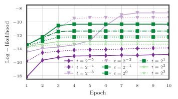
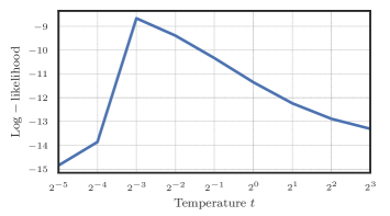
Figure 1: Relation between learning and temperature. (left) Training log-likelihoods over number of training epochs. Highest log-likelihoods are achieved for medium temperatures $t$ while low and high temperatures result in decreased log-likelihoods. (right) Log-likelihoods after convergence over temperature $t$. The highest log-likelihood is achieved for temperature $t=2^{-3}$.

5.3 Product Recommendation

We consider the Amazon baby registry data Gillenwater et al. (2014). The data consists of baby registry data collected from Amazon and split into several datasets according to product categories, e.g. safety, strollers, etc. The datasets contain $5{,}500$ to $13{,}300$ registries of users. The data is processed using 10-fold cross-validation. As for PD²Greedy the order of items matters, we permute the items according to their empirical frequencies for each dataset.

For every dataset and fold, we fit a facility location diversity (FLID) type model Tschiatschek et al. (2016), i.e.

$$f(S)=\sum_{i\in S}u_{i}+\underbrace{\sum_{d=1}^{D}\big{(}\max_{i\in S}w_{i,d}-\sum_{i\in S}w_{i,d}\big{)}}_{\textnormal{div}(S)},$$

where $u_{i}\in\mathbb{R}$ encodes the utility of product $i$ and $w_{i,d}\in\mathbb{R}_{\geq 0}$ encodes the $d$th latent property of item $i$. The intuitive idea behind the term $\textnormal{div}(S)$ is to encode repulsive dependencies between items that all have the $d$th latent property.

We train FLID models by optimizing the likelihood of the training data in Equation (2) for $t=1$ and the sigmoid approximation (FLID^D) and by optimizing the likelihood in Equation (4) (FLID^G) for $t=0.1$. For optimization we used Adam with a batch size of $1$ for FLID^D and with a batch size of $100$ for FLID^G. We exhaustively computed the sum in Equation (4) for sets with at most 5 items and otherwise approximated this sum by randomly selecting $5!$ of the summands (and scaling the result accordingly). We decayed the initial learning rate of $0.01$ with a decay factor of $0.9$ per epoch. We trained all models for 20 epochs. The number of latent dimensions $D$ is chosen as 10 for ground sets with at most 40 items and 20 for larger ground sets.

Performance evaluation. To assess the performance of our trained models we compute the following performance measures and compare them to the performance of modular models (fully factorized models independently predicting the inclusion of any element in a set without considering correlations) and determinantal point process (DPPs) fitted by expectation maximization Gillenwater et al. (2014). Let $\mathcal{D}=\{R_{1},\ldots,R_{N}\}$ be a set of registries and let $\bar{\mathcal{D}}=\{R\in\mathcal{D}\mid|R|>1\}$ be the set of registries in $\mathcal{D}$ with at least 2 items.

• Relative improvement in likelihood rLL. This measure quantifies the increase in likelihood for FLID and DPPs over a modular model. The rLL is computed as

  $$\textsc{rLL}=\frac{|\sum_{R\in\mathcal{D}}\log P(R)-\textnormal{LL}_{\textnormal{mod}}|}{\textnormal{LL}_{\textnormal{mod}}},$$

  where $P(R)$ is the probability of $R$ for FLID/DPP and $\textnormal{LL}_{\textnormal{mod}}=\sum_{R\in\mathcal{D}}\log P_{\textnormal{modular}}(R)\log$ is the likelihood of the fully factorized model.

• Fill-in accuracy Acc. We test how accurately the considered models can predict items removed from a baby registry. We compute the fill-in accuracy as

  $$\textsc{Acc}(\mathcal{D};\hat{f})=\frac{1}{|\bar{\mathcal{D}}|}\sum_{R=\{r_{1},\ldots,r_{k}\}\in\bar{\mathcal{D}}}\sum_{i=1}^{k}\mathbf{1}_{\hat{f}(R-{r_{i}})=r_{i}}$$

  where $\hat{f}$ is the function used for prediction. For FLID and modular functions, $\hat{f}(S)=\arg\max_{e\in\mathcal{V}\setminus S}P(S+e)$. In the case of DPPs, $\hat{f}$ returns the element with largest marginal conditioned on $S$.

• Mean reciprocal rank MRR. Instead of only accounting correct predictions, this measure considers the order in which the models would predict items. Formally, MRR is defined as

  $$\textsc{MRR}(\mathcal{D};\hat{f})=\frac{1}{|\bar{\mathcal{D}}|}\sum_{R=\{r_{1},\ldots,r_{k}\}\in\bar{\mathcal{D}}}\sum_{i=1}^{k}\frac{1}{r(r_{i};R-{r_{i}})},$$

  where $r(r_{i};R-r_{i})=k$ if the item $r_{i}$ would be predicted as the $k$th item.

The results are shown in Table 2. We observe that FLID in most cases outperforms the modular model. The rLL of DPPs is in general higher than that of FLID^D. In many cases FLID^G significantly outperforms DPPs and FLID^D in terms of fill-in accuracy and MRR.

	rLL [%]		Acc [%]				MRR [–]
Dataset	DPP	FLIDD	modular	DPP	FLIDD	FLIDG	modular	DPP	FLIDD	FLIDG
safety	$11.60$	$12.47$	$16.06$	$16.20$	$16.67$	$16.72$	$29.55$	$30.02$	$30.34$	$30.36$
carseats	$8.77$	$8.78$	$13.76$	$14.72$	$15.03$	$16.18$	$28.75$	$30.14$	$30.56$	$31.33$
strollers	$8.54$	$9.58$	$14.42$	$16.79$	$19.69$	$21.75$	$27.36$	$29.90$	$32.95$	$34.49$
furniture	$10.53$	$10.59$	$15.82$	$16.08$	$15.93$	$17.21$	$30.11$	$30.73$	$30.35$	$31.21$
health	$2.89$	$1.83$	$9.94$	$10.32$	$10.30$	$12.07$	$21.42$	$22.31$	$21.87$	$23.26$
bath	$2.66$	$1.65$	$7.30$	$8.68$	$8.24$	$9.90$	$16.06$	$17.32$	$17.13$	$18.88$
media	$2.35$	$1.19$	$9.31$	$10.07$	$10.04$	$14.31$	$20.29$	$21.70$	$21.86$	$26.14$
toys	$2.22$	$1.04$	$9.85$	$11.65$	$11.59$	$14.78$	$21.93$	$23.40$	$23.64$	$26.23$
bedding	$1.55$	$0.24$	$17.17$	$17.43$	$16.87$	$17.53$	$27.59$	$28.04$	$27.59$	$28.01$
apparel	$0.93$	$0.00$	$13.47$	$13.30$	$13.31$	$13.28$	$20.88$	$21.19$	$21.16$	$22.00$
diaper	$0.90$	$0.25$	$10.13$	$10.13$	$10.24$	$14.55$	$18.03$	$18.56$	$19.10$	$23.78$
gear	$1.68$	$0.56$	$6.23$	$6.34$	$6.10$	$6.46$	$14.80$	$15.12$	$14.66$	$14.71$
feeding	$0.17$	$0.00$	$6.38$	$6.77$	$6.49$	$9.24$	$14.53$	$15.22$	$15.02$	$18.00$

Table 2: Performance of different models on the Amazon baby registry dataset. Performance of log-modular models fitted with maximum likelihood (modular), DPPs trained with the EM algorithm (DPP), FLID trained with PD²Greedy (FLID^D), and FLID trained with PGreedy (FLID^G). FLID^D, FLID^Gand DPPs clearly outperform the modular model in most cases. FLID^Goutperforms FLID^Dand DPPs in many cases in terms of fill-in accuracy and MRR. rLL is omitted for FLID^Gas it would require approximation due to the intractability of (4) for large sets. A rLL of $0.00$ indicates a negative likelihood improvement.

5.4 Image Collection Summarization

We consider the problem of image collection summarization, i.e. the problem of selecting a subset of images $S$ of an image collection $\mathcal{V}$ such that the selected images summarize the content of the collection $\mathcal{V}$ well (e.g. $S$ covers all important scenes in $\mathcal{V}$ and the pictures in $S$ are diverse).

Data. We use the image collection summarization data from Tschiatschek et al. (2014). This data consists of 14 image collections $\mathcal{V}_{1},\ldots,\mathcal{V}_{14}$, each consisting of 100 images, i.e. $\mathcal{V}_{i}=\{I^{(i)}_{1},\ldots,I^{(i)}_{100}\}$. The images capture diverse themes, e.g. traveling, shopping, etc. For each image collection $i$, hundreds of human generated summaries were collected. We heuristically prune the original human summaries using the technique proposed in Tschiatschek et al. (2014). The remaining human summaries $\mathcal{H}^{(i)}=\{H^{(i)}_{1},\ldots,H^{(i)}_{N_{i}}\}$ are considered as approximate maximizers of an unknown function $f(S\mid\mathcal{V}_{i})$ that we want to learn.

Evaluation, model, training. We follow the evaluation from Tschiatschek et al. (2014); Dolhansky and Bilmes (2016). That is, we train our model on 13 of the 14 image collections and test the model on the held out image collection. We report the average VROUGE score Tschiatschek et al. (2014) on the hold out image collection. The VROUGE score quantifies the quality of a summary for an image collection, capturing notions of coverage and diversity.

We train a model using the visual features computed in Tschiatschek et al. (2014), similar as in Dolhansky and Bilmes (2016). Our model processes the 628 dimensional feature vector of each image $i$ by first compressing them into 100 dimensional vectors $h_{i}$ by a fully connected layer with ReLU activations. From this intermediate representation we compute a quality score $q_{i}$ for every image $i$ by another fully connected layer. From the intermediate representation we also compute means, maxes and variances across the images for every feature. These quantities are transformed into a threshold vector $b$ through another fully connected layer with ReLU activation ($b$ is 100 dimensional as the intermediate representation). The qualities, the threshold vector and intermediate representations parameterize a set function $f(S)=\sum_{i\in S}q_{i}+\sum_{j=1}^{100}\min(b_{i},\sum_{i\in S}h_{i,j})$. We use dropout to avoid overfitting.

We optimize the expected VROUGE score induced by our proposed algorithm PGreedy, using a temperature of $t=1$ and randomly sampled permutations of the items in the training samples (all human generated summaries consist of 10 images and hence computing the exact expected VROUGE score using (4) is infeasible). For optimization, we used Adam Kingma and Ba (2015) with a learning rate of $0.001$ and weight decay selected via cross-validation.

Results. We achieve an average normalized VROUGE score of 0.81. This is comparable to the performance achieved in Dolhansky and Bilmes (2016). The authors in Tschiatschek et al. (2014) achieved an average VROUGE score of 1.13 for their best model by learning a mixture of more than 500 hand specified component functions. In our experiments, we observed that our model easily overfits the training data. So more elaborate regularization methods could potentially improve the performance of our model further.

6 Related Work

While traditionally deep neural nets are used to learn parameters for a fixed size input vector, there is a growing literature on learning parameters of set functions with deep neural nets. For instance, Rezatofighi et al. (2017) considers learning the parameters of the likelihood of a set using deep neural nets and  Zaheer et al. (2017) designs specific layers to create permutation invariant and equivariant functions for set prediction.

Balcan and Harvey (2011) considers learning submodular functions in a PAC-style framework and provides lower bounds on their learnability.  Lin and Bilmes (2012); Tschiatschek et al. (2014) learn mixtures of submodular functions by optimizing the weights using a large margin structured prediction framework. Since only the weights, not the components, are learned, the learning process is highly dependent on the representativeness of the functions used.  Dolhansky and Bilmes (2016) develop a new class of submodular functions, similar to deep neural nets, and learn them in a maximum margin setting.

Recently, there has been some applications which combine deep learning and reinforcement learning to develop heuristics for combinatorial optimization problems. For instance, Khalil et al. (2017) uses graph embeddings and reinforcement learning to learn heuristics for graph combinatorial optimization problems such as maximum cut.

7 Conclusions

We considered learning of submodular functions which are used for subset selection through greedy maximization. To this end, we proposed variants of two types of greedy algorithms that allow for approximate maximization of submodular set functions such that their output can be interpreted as a distribution over sets. This distribution is differentiable, can be used within deep learning frameworks and enables gradient based learning. Furthermore, we theoretically characterized the tradeoff of smoothness and accuracy of some of the considered algorithms. We demonstrated the effectiveness of our approach on different applications, including max-cuts and product recommendation—observing good empirical performance.

Appendix A Proof of the Approximation Guarantee for Softplus Approximation (Theorem 1)

Proof.

This proof closely follows the proof of Theorem $1.2$ in  Buchbinder et al. [2015]. We show below that for $t\leq\tfrac{\epsilon}{\log(2)}$ the following holds:

$$\mathbb{E}[f(\textnormal{OPT}_{i-1})-f(\textnormal{OPT}_{i})]\leq$$ (5)

$$\qquad\frac{1}{2}\mathbb{E}[f(X_{i})-f(X_{i-1})+f(Y_{i})-f(Y_{i-1})]+\epsilon$$

Summing over $i$ we get a telescopic sum. Collapsing it, we get

$$\mathbb{E}[f(\textnormal{OPT}_{0})-f(\textnormal{OPT}_{n})]=f(\textnormal{OPT})-\mathbb{E}[f(X_{n})]$$

$$\qquad\leq\frac{1}{2}\mathbb{E}[f(X_{n})-f(X_{0})+f(Y_{n})-f(Y_{0})]+n\epsilon$$

$$\qquad\leq\mathbb{E}[f(X_{n})]+n\epsilon.$$

Consequently,

$$\mathbb{E}[f(X_{n})]\geq\frac{f(\textnormal{OPT})}{2}-\frac{n}{2}\epsilon.$$

We still need to prove inequality (5). We first bound the left hand side and rewrite the right hand side of (5):

1. LHS:

   $$\mathbb{E}[f(\textnormal{OPT}_{i-1})-f(\textnormal{OPT}_{i})]\leq\max\{p_{a}b,p_{b}a\},$$

   where $p_{a}=\frac{a^{\prime}}{a^{\prime}+b^{\prime}}$ and $p_{b}=1-p_{a}$.

2. RHS:

   $$\frac{1}{2}\mathbb{E}[f(X_{i})-f(X_{i-1})+f(Y_{i})-f(Y_{i-1})]$$

   $$\qquad=\frac{1}{2}(p_{a}a+p_{b}b).$$

Hence, to conclude with the statement of the theorem, it is sufficient to prove that $\max(\frac{a^{\prime}b}{a^{\prime}+b^{\prime}},\frac{ab^{\prime}}{a^{\prime}+b^{\prime}})\leq\frac{1}{2}(\frac{a^{\prime}a}{a^{\prime}+b^{\prime}}+\frac{b^{\prime}b}{a^{\prime}+b^{\prime}})+\epsilon$ for $t\leq\tfrac{\epsilon}{\log(2)}$. W.l.o.g, assume $a^{\prime}b\geq ab^{\prime}$. Then there are the following cases:

• Case 1. $a,b\geq 0$. Let $\delta_{a}=a^{\prime}-a$ and $\delta_{b}=b^{\prime}-b$. Note that $\delta_{a}\leq t\log(2)$. Hence:

  $$\epsilon\geq t\log(2)\geq t\log(2)\frac{b}{a^{\prime}+b^{\prime}}$$

  $$\Rightarrow\delta_{a}b\leq\epsilon(a^{\prime}+b^{\prime})$$

  $$\Rightarrow(a+\delta_{a})b-\frac{1}{2}(a+\delta_{a})a-\frac{1}{2}(b+\delta_{b})b\leq\epsilon(a^{\prime}+b^{\prime})$$

  $$\Leftrightarrow\max(\frac{a^{\prime}b}{a^{\prime}+b^{\prime}},\frac{ab^{\prime}}{a^{\prime}+b^{\prime}})\leq\frac{1}{2}(\frac{a^{\prime}a}{a^{\prime}+b^{\prime}}+\frac{b^{\prime}b}{a^{\prime}+b^{\prime}})+\epsilon$$

• Case 2. $a\leq 0,b\geq 0$. Since $a\leq 0$, $a^{\prime}>0$ and $b\geq 0$, $b^{\prime}\geq t\log(2)$. Thus, $a^{\prime}+b^{\prime}>t\log(2)$

  We can rewrite the statement that is sufficient to prove as $2a^{\prime}b\leq a^{\prime}a+b^{\prime}b+\epsilon^{\prime}$ with $\epsilon^{\prime}=2\epsilon t\log(2)\leq 2\epsilon(a^{\prime}+b^{\prime})$. Equivalently:

  $$0\leq a^{\prime}a-2a^{\prime}b+b^{\prime}b+\epsilon^{\prime}$$

  $$\Leftrightarrow 0\leq(a^{\prime}-b^{\prime})^{2}-(a^{\prime}-b^{\prime})^{2}+a^{\prime}a-2a^{\prime}b+b^{\prime}b+\epsilon^{\prime}$$

  $$\Leftrightarrow 0\leq(a^{\prime}-b^{\prime})^{2}+a^{\prime}(a-a^{\prime})+2a^{\prime}(b^{\prime}-b)$$

  $$\qquad+b^{\prime}(b-b^{\prime})+\epsilon^{\prime}$$

  The first and third term are non-negative. We show that $t\leq\tfrac{\epsilon}{\log(2)}$ is sufficient for the second and the fourth term to be not smaller than $-\epsilon^{\prime}/2$.

  • For the second term we need $-\epsilon^{\prime}/2\leq a^{\prime}(a-a^{\prime})$. Observe that

    $$a-a^{\prime} =t\log(\exp(a/t))-t\log(1+\exp(a/t))$$

    $$=-t\log(1+\exp(-a/t)).$$

    Hence we need $-\epsilon^{\prime}/2\leq-a^{\prime}t\log(1+\exp(-a/t))$. Observe that $\log(1+\exp(a/t))\log(1+\exp(-a/t))$ has maximum value $\log(2)^{2}$. Thus it is sufficient to ensure that $-\epsilon^{\prime}/2\leq-t^{2}\log(2)^{2}$. Note that $\epsilon^{\prime}=2\epsilon t\log(2)$ and hence $t\leq\tfrac{\epsilon}{\log(2)}$ is sufficient.

  • The argument for the fourth term is analogeous to the one above, showing that $t\leq\tfrac{\epsilon}{\log(2)}$ is sufficient to prove our statement.

  It is hence sufficient to have $t\leq\tfrac{\epsilon}{\log(2)}$.

• Case 3. $a\geq 0,b\leq 0$. This violates the assumption that $a^{\prime}b\geq ab^{\prime}$.

• Case 4. $a\leq 0,b\leq 0$. Contradiction, since because of submodularity $a+b\geq 0$.

∎

Appendix B Proof of the Approximation Guarantee for Sigmoid Approximation (Theorem 2)

Proof.

This proof closely follows the proof of Theorem $1.1$ in  Buchbinder et al. [2015].

We show below that for $t<\tfrac{3\epsilon}{|\mathcal{V}|W(1/e)}$ the following holds:

$$\mathbb{E}[f(\textnormal{OPT}_{i-1})-f(\textnormal{OPT}_{i})]\leq$$ (6)

$$\qquad\mathbb{E}[f(X_{i})-f(X_{i-1})+f(Y_{i})-f(Y_{i-1})]+\epsilon,$$

From this it then follows that

$$\mathbb{E}[f(\textnormal{OPT}_{0})-f(\textnormal{OPT}_{n})]=f(\textnormal{OPT})-\mathbb{E}[f(X_{n})]$$

$$\qquad\leq\mathbb{E}[f(X_{n})-f(X_{0})+f(Y_{n})-f(Y_{0})]+n\epsilon$$

$$\qquad\leq 2\mathbb{E}[f(X_{n})]+n\epsilon.$$

Consequently,

$$\mathbb{E}[f(X_{n})]\geq\frac{f(\textnormal{OPT})}{3}-\frac{n}{3}\epsilon.$$

To prove the inequality (6), observe that:

1. LHS:

   $$\mathbb{E}[f(\textnormal{OPT}_{i-1})-f(\textnormal{OPT}_{i})]\leq\max\{p_{a}b,p_{b}a\},$$

   where $p_{a}=\sigma(a-b)$ and $p_{b}=1-p_{a}$.

2. RHS:

   $$\mathbb{E}[f(X_{n})-f(X_{0})+f(Y_{n})-f(Y_{0})]=p_{a}a+p_{b}b.$$

We consider three cases to prove $\max\{p_{a}b,p_{b}a\}\leq p_{a}a+p_{b}b+\epsilon$ which is equivalent to $\max\{\sigma(a-b)b,\sigma(b-a)a\}\leq\sigma(a-b)a+\sigma(b-a)b+\epsilon$:

• Case 1. $a,b\geq 0$. If $a\geq b$, $\sigma(a-b)\geq 0.5$ and $a-b\geq 0$. Thus,

  $$0 =0.5(a-b)+0.5(b-a)$$

  $$\leq\sigma(a-b)(a-b)+\sigma(b-a)(b-a).$$

  This implies

  $$\sigma(a-b)a+\sigma(b-a)b\geq p_{a}b+p_{a}b\geq\max\{p_{a}b,p_{b}a\}.$$

  For $a\leq b$ the same argumentation holds.

• Case 2. $a\geq 0,b\leq 0$. In this case $\max\{p_{a}b,p_{b}a\}=p_{b}a$ and $\sigma(a-b)\geq 0.5$. Hence we need find $\epsilon$ such that

  $$0\leq\sigma(a-b)a+\underbrace{\sigma(b-a)(b-a)}_{g(a,b)}+\epsilon$$ (7)

  is satisfied to prove the above inequality. Note that the first term can be minimized by setting $a=0$ (which is always possible as the second term only depends on the difference $b-a$ and the third term is independent of both $a$ and $b$). Minimizing the term $g(a,b)$, which can be written as $g(x)=-\frac{1}{(1+e^{x/t})}x$ with $x=a-b$ yields that the minimum is achieved at $x^{*}=tW(1/e)+t$ and evaluates to $g(x^{*})=-tW(1/e)$, where $W$ is the Lambert-W function. Thus, having $t\leq\tfrac{1}{W(1/e)}\epsilon$ ensures that the desired inequality holds.

• Case 3. $a\leq 0,b\geq 0$. Analogous to above.

∎

References

- Bahdanau et al. [2014] Dzmitry Bahdanau, Kyunghyun Cho, and Yoshua Bengio. Neural machine translation by jointly learning to align and translate. CoRR, abs/1409.0473, 2014.
- Balcan and Harvey [2011] Maria-Florina Balcan and Nicholas J. A. Harvey. Learning submodular functions. In Symposium on Theory of Computing (STOC), pages 793–802, 2011.
- Buchbinder et al. [2015] Niv Buchbinder, Moran Feldman, Joseph Seffi, and Roy Schwartz. A tight linear time (1/2)-approximation for unconstrained submodular maximization. SIAM Journal on Computing, 44(5):1384–1402, 2015.
- Djolonga and Krause [2014] Josip Djolonga and Andreas Krause. From map to marginals: Variational inference in bayesian submodular models. In Advances in Neural Information Processing Systems (NIPS), pages 244–252. 2014.
- Dolhansky and Bilmes [2016] Brian W Dolhansky and Jeff A Bilmes. Deep submodular functions: Definitions and learning. In Advances in Neural Information Processing Systems (NIPS), pages 3404–3412, 2016.
- Felzenszwalb et al. [2010] Pedro F Felzenszwalb, Ross B Girshick, David McAllester, and Deva Ramanan. Object detection with discriminatively trained part-based models. TPAMI, 32(9):1627–1645, 2010.
- Gillenwater et al. [2014] Jennifer A Gillenwater, Alex Kulesza, Emily Fox, and Ben Taskar. Expectation-maximization for learning determinantal point processes. In Advances in Neural Information Processing Systems (NIPS), pages 3149–3157. 2014.
- Gurobi Optimization [2016] Inc. Gurobi Optimization. Gurobi optimizer reference manual, 2016.
- Khalil et al. [2017] Elias Khalil, Hanjun Dai, Yuyu Zhang, Bistra Dilkina, and Le Song. Learning combinatorial optimization algorithms over graphs. In Advances in Neural Information Processing Systems, pages 6351–6361, 2017.
- Kingma and Ba [2015] Diederik P Kingma and Jimmy Ba. Adam: A method for stochastic optimization. International Conference for Learning Representations (ICLR), 2015.
- Lin and Bilmes [2010] Hui Lin and Jeff Bilmes. Multi-document summarization via budgeted maximization of submodular functions. In Conference of the North American Chapter of the Association for Computational Linguistics, pages 912–920. Association for Computational Linguistics, 2010.
- Lin and Bilmes [2012] Hui Lin and Jeff Bilmes. Learning mixtures of submodular shells with application to document summarization. In Conference on Uncertainty in Artificial Intelligence (UAI), pages 479–490. AUAI Press, 2012.
- Nemhauser et al. [1978] George L Nemhauser, Laurence A Wolsey, and Marshall L Fisher. An analysis of approximations for maximizing submodular set functions—i. Mathematical Programming, 14(1):265–294, 1978.
- Ren et al. [2015] Shaoqing Ren, Kaiming He, Ross Girshick, and Jian Sun. Faster r-cnn: Towards real-time object detection with region proposal networks. In C. Cortes, N. D. Lawrence, D. D. Lee, M. Sugiyama, and R. Garnett, editors, Advances in Neural Information Processing Systems (NIPS), pages 91–99. Curran Associates, Inc., 2015.
- Rezatofighi et al. [2017] S Hamid Rezatofighi, Anton Milan, Ehsan Abbasnejad, Anthony Dick, Ian Reid, et al. Deepsetnet: Predicting sets with deep neural networks. In International Conference on Computer Vision (ICCV), pages 5257–5266. IEEE, 2017.
- Tschiatschek et al. [2014] Sebastian Tschiatschek, Rishabh K Iyer, Haochen Wei, and Jeff A Bilmes. Learning mixtures of submodular functions for image collection summarization. In Advances in neural information processing systems (NIPS), pages 1413–1421, 2014.
- Tschiatschek et al. [2016] Sebastian Tschiatschek, Josip Djolonga, and Andreas Krause. Learning probabilistic submodular diversity models via noise contrastive estimation. In Artificial Intelligence and Statistics (AISTATS), pages 770–779, 2016.
- Tschiatschek et al. [2018] Sebastian Tschiatschek, Aytunc Sahin, and Andreas Krause. Differentiable submodular maximization. arXiv preprint arXiv:1803.01785, 2018.
- Wang et al. [2013] Jun Wang, Tony Jebara, and Shih-Fu Chang. Semi-supervised learning using greedy max-cut. Journal of Machine Learning Research, 14(1):771–800, 2013.
- Zaheer et al. [2017] Manzil Zaheer, Satwik Kottur, Siamak Ravanbakhsh, Barnabas Poczos, Ruslan R Salakhutdinov, and Alexander J Smola. Deep sets. In Advances in Neural Information Processing Systems, pages 3394–3404, 2017.
- Zhang et al. [2016] Ke Zhang, Wei-Lun Chao, Fei Sha, and Kristen Grauman. Video summarization with long short-term memory. In European Conference on Computer Vision, pages 766–782. Springer, 2016.