Theory of magnetoelastic resonance in a mono-axial chiral helimagnet

Abstract

We study magnetoelastic resonance phenomena in a mono-axial chiral helimagnet belonging to hexagonal crystal class. By computing the spectrum of coupled elastic wave and spin wave, it is demonstrated how hybridization occurs depending on their chirality. Specific features of the magnetoelastic resonance are discussed for the conical phase and the soliton lattice phase stabilized in the mono-axial chiral helimagnet. The former phase exhibits appreciable non-reciprocity of the spectrum, the latter is characterized by a multi-resonance behavior. We propose that the non-reciprocal spin wave around the forced-ferromagnetic state has potential capability to convert the linearly polarized elastic wave to circularly polarized one with the chirality opposite to the spin wave chirality.

I Introduction

Many recent studies have focused on physical properties of chiral helimagnets (CHM). It is widely recognized that coupling of lattice degrees of freedom with magnetism plays a significant role in this class of materials. For example, the cubic chiral helimagnet MnSiFawcett1970 ; Matsunaga1982 exhibits the anomalies in the thermal expansion coefficient and similarly MnGeValkovskiy2016 exhibits magnetic peculiarities connected with distortion of the B20 structure upon heating.

Magnetoelastic interaction may contribute either to dynamic elastic deformations that affect significantly the dynamics of magnetic moments or to static strains, which in turn influence the dispersion and band-gaps of the coupled magnetoelastic waves. This coupling was argued in relation to a possible structural transition in Mn_1-xFe_xGe solid solutions Makarova2012 ; Dyadkin2014 ; Martin2016 . Early theoretical studies of the magnetoelastic interaction in cubic helimagnets with B20 structure predicted an appearance of non-analytical wave-vector dependence for the static susceptibility as a result of magnetization-induced inhomogeneous strains Plumer1982 ; Plumer1984 ; it was demonstrated that this interaction tends to disrupt the assumed helical structure Maleyev2009 .

One of the powerful tools to investigate specific features of the magnetoelastic coupling are ultrasound measurements, where characteristics of propagation of high-frequency elastic waves are indicated by a dependence of the velocity and attenuation of the ultrasonic waves on magnetic properties of the solid. They are reputed to be a valuable probe to investigate magnetic phase transitions in MnSi due to high sensitivity and accuracy Petrova2009 ; Petrova2016 . Sound velocities measured in these studies are highly sensitive to local values of elastic constants and their evaluation does not involve any sophisticated experimental technique.

One of the most important reasons of keen interest in chiral helimagnets is driven by the unique soliton-like forms of magnetic order revealed in these materials: the chiral soliton lattice (CSL) actually observed in CrNb₃S₆ Togawa2012 and the skyrmion lattice found, for example, in MnSi, (Fe,Co)Si and Cu₂OSeO₃ Binz2009 ; Yu2010 ; Adams2010 ; Seki2012 . Ultrasonic measurements being compared with magnetic and electric ones demonstrate clear advantages for exploring these topological objects: they are not restricted by electric conductivity of a material; due to magnetoelastic interaction, they provide insight into anisotropic properties of the magnetic lattices by comparing different elastic modes; lastly, they make possible to determine directly elasticity and viscosity of these lattices as a result of the magnetoelastic coupling. Mechanical control of the skyrmion lattice phase demonstrated in a bulk MnSi single crystal is of considerable interest; it is achieved with a mechanical stress and a low energy cost Nii2015 . Deep understanding of the issue is vital for potential applications in technology.

A growing interest in the nontrivial topological phases of the chiral helimagnets dictates an urgent need to elaborate an appropriate formalism of the magnetoelastic interaction of these materials. The seminal theory of magnetoelastic waves in ferromagnetic crystals, originally suggested by Kittel Kittel1958 , has been expanded into the class of helimagnets with the Dzyaloshinskii-Moryia (DM) exchange coupling over few decades ago Stefanovski1969 ; Vlasov1973 . However, spontaneous deformations in a ground state were ignored in these treatments. The theory developed in Ref. Turov1983 overcame this drawback; a pertinent investigation for the conical phase of the relativistic spiral has been later reported Shavrov1989 ; Bychkov1990 . Recently this problem has been under new scrutiny in the light of of magnetoelectric hexaferrites, where the magnetoelastic resonance is largely the same as for the phase of forced ferromagnetism in the monoaxial CHM Vittoria2015 . We also point out a remarkable feature of spin wave propagation in the conical phase in chiral helimangets. A preferable spin-wave helicity (left-handed or right-handed) is fixed by the DM interaction. Consequently, non-reciprocal magnon transport is realized.Iguchi2015 ; Seki2015

The coupling between acoustic phonons and magnons was incorporated to explore the effects of the spin-lattice coupling in the topologically nontrivial skyrmion lattice in MnSi and MnGe Zhang2017 . The magnetoelastic interaction results from expanding the strengths of both Heisenberg exchange interaction and the Dzyaloshinskii-Moriya interaction up to the linear order of phonon degrees of freedom. Efficiency of such a form of the magnetoelastic coupling was experimentally demonstrated for the skyrmion lattice in MnGe, where the elastic response is an order of magnitude larger than the conventional case (for example, in MnSi) was reported Kanazawa2016 . To calculate ultrasonic responses in MnSi the thermodynamical model was used Hu2017 , which incorporates a magnetoelastic functional with necessary high-order interactions allowed by group theory. Unfortunately, a progress in this direction is severely hampered by lack of a generally accepted theoretical model for the skyrmion lattice phase Rosch2016 .

In this paper, we fill a gap coming from, to the best of our knowledge, an absence of a theory of magnetoelastic interactions in the chiral soliton lattice. This case is certainly of a special interest: a control of the period of the soliton lattice by means of an external magnetic field enables governing a resonant frequency in a substantial way. Our analysis is intended for crystals of the hexagonal symmetry which the real prototype compound CrNb₃S₆ belongs to. Until now, only the case of the exchange spiral has been investigated for this symmetry Bychkov1990 . A spiral magnetic order owing to the DM interaction was previously analyzed for a media with isotropic elastic and magnetoelastic properties Shavrov1993 that can be applied to the chiral magnetic materials of cubic symmetry, MnSi and FeGe. The aim of our investigation is to find out specific features of magnetoelastic resonance in the magnetic soliton lattice and to provide insight into factors that affect the process significantly. In addition, we revisit a case of the conical phase to discuss salient non-reciprocity effects in propagation of magnetoelastic waves.

The paper is organized as follows. In Sec. II, the model of the interaction between the magnetic and the elastic degrees of freedom is formulated. Sec. III provides a treatment of the magnetostriction problem, i.e., a calculation of elastic deformations caused by magnetization of the soliton lattice. In Sec. IV, the coupled system of dynamical equations for the lattice and the spin variables is solved; the spectrum of the magnetoelastic waves is analyzed. For the sake of simplicity, we consider the waves traveling along a principal axis of the crystal. In Sec. V, the conclusions are presented.

II The model

We consider a hexagonal chiral helimagnet, where a modulated magnetic ordering characterized by the magnetization $\boldsymbol{M}(z,t)$, is stabilized along the symmetry direction taken further as $z$-axis. In hexagonal crystals, the total energy density, which takes into account interaction with elastic deformations, can be expressed in the following form

$$\mathcal{F}=\frac{J}{2}\left(\partial_{z}\boldsymbol{M}\right)^{2}+D\hat{z}\cdot\left[\boldsymbol{M}\times\partial_{z}\boldsymbol{M}\right]-\boldsymbol{H}\cdot\boldsymbol{M}+\mathcal{F}_{ME}+\mathcal{F}_{E},$$ (1)

where the first term is that of the Heisenberg model with the ferromagnetic exchange coupling $J$; the second terms is the DM interaction of the strength $D$, and the third one describes the interaction of the magnetization with the external magnetic field $\boldsymbol{H}$. The last two terms stand for the magnetoelastic and elastic energy densities respectively, whose explicit form for the hexagonal crystal structure is given by Mason1954

$$\mathcal{F}_{E} =\frac{c_{11}}{2}\left(u_{xx}^{2}+u_{yy}^{2}\right)+\frac{c_{33}}{2}u_{zz}^{2}+\left(c_{11}-c_{12}\right)u_{xy}^{2}$$

$$+c_{12}u_{xx}u_{yy}+2c_{44}\left(u_{xz}^{2}+u_{yz}^{2}\right)+c_{13}\left(u_{xx}+u_{yy}\right)u_{zz},$$ (2)

$$\mathcal{F}_{ME} =\left(b_{11}-b_{12}\right)\left(u_{xx}M_{x}^{2}+2u_{xy}M_{x}M_{y}+u_{yy}M_{y}^{2}\right)$$

$$+\left(b_{13}-b_{12}\right)\left(u_{xx}+u_{yy}\right)M_{z}^{2}+\left(b_{33}-b_{31}\right)u_{zz}M_{z}^{2}$$

$$+2b_{44}\left(u_{xz}M_{x}M_{z}+u_{yz}M_{y}M_{z}\right),$$ (3)

where $u_{ij}$ is the deformation tensor defined in terms of elastic deformations $s_{i}$

$$u_{ij}=\frac{1}{2}\left(\frac{\partial s_{i}}{\partial x_{j}}+\frac{\partial s_{j}}{\partial x_{i}}\right).$$ (4)

where $i,j=x,y,z$ indicate directions schematically shown in Fig. 1 (a), and $b_{ij}$ and $c_{ij}$ are correspondingly the magnetoelastic and the elastic stiffness modulus constants.

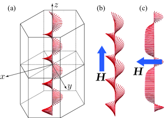
Figure 1: (color online) The coordinate system for a hexagonal crystal with a magnetic spiral inside used throughout the paper (a); schematic pictures of the magnetic ordering for the conical phase (b) and the soliton lattice phase (c).

To study the magnetoelastic resonance, we consider the coupled equations of motion for $\boldsymbol{M}$ and $u_{ij}$

$$\rho\frac{\partial^{2}s_{i}}{\partial t^{2}} =\frac{\partial\sigma_{ij}}{\partial x_{j}},$$ (5)

$$\frac{\partial\boldsymbol{M}}{\partial t} =-\gamma\boldsymbol{M}\times\boldsymbol{H}_{\mathrm{eff}},$$ (6)

where both the effective field $\boldsymbol{H}_{\mathrm{eff}}=-\delta\mathcal{F}/\delta\boldsymbol{M}$ and the stess tensor $\sigma_{ij}=\left(1+\delta_{ij}\right)/2\left(\partial\mathcal{F}/\partial u_{ij}\right)$Comstock1963 are defined by the energy density in Eq. 1, $\rho$ is the crystal mass density, and $\gamma$ denotes the gyromagnetic ratio. For numerical estimations later on, we use the crystallographic data for CrNb₃S₆ compound, which contains 20 atoms per unit cell: twelve S atoms, six Nb atoms and two intercalated Cr atoms. The unit cell parameters are $a=5.741\mathring{A}$ and $c=12.101\mathring{A}$ that yields $\rho=5.029$ g/cm³. Mandrus2013 For a numerical value of the magnetization $M_{0}$, we use the result $3.2\,\mu_{B}/$Cr and the nearest Cr-Cr distance in the $ab$-plane (5.741 $\mathring{A}$) and along the $c$-axis (6.847 $\mathring{A}$). Mandrus2013 This gives $M_{0}=131.5$ kA/m = 1649 Gs.

At present, it is hard to give any precise numerical values for the coefficients $b_{ij}$ and $c_{ij}$ in the prototype compound, chiral helimagnet CrNb₃S₆. Instead, the values of the stiffness moduli for the parent matrix NbS₂ of the same hexagonal structure are used: $c_{11}=148$ GPa, $c_{12}=51$ GPa, $c_{13}=1$ GPa, $c_{33}=c_{44}=2$ GPa Gaillac2016 . The constants $b_{ij}M_{0}^{2}$ of the order $1-10\,\text{MPa}$ are used for estimations whenever it is necessary.

We emphasize, that in order to develop a linear theory of magnetoelastic resonance in systems with inhomogeneous magnetization profile, it is important to take into account the magnetostricrive effect from the magnetization background Turov1983 , which results into the inhomogenious deformation fied $u^{(0)}_{ij}(\boldsymbol{r})$ in the ground state induced by the spontaneous magnetization $\boldsymbol{M}_{0}(\boldsymbol{r})$. Interestingly, as it was pointed out in Ref. [Turov1983, ], this effect of spontaneous symmetry breaking caused by magnetic ordering in a system of the two coupled fields is analogous to the Higgs effect in the theory of elementary particles Higgs1964 . The spatial dependence of the background magnetization also requires modification of methods used in previous studies of ferromagnetic materials. For example, nonunifrom strains can make all the magnetoelastic waves to be massless Goldstone’s modes, i.e., in contrast to ferromagnets, no magnetoelastic gap appears. Shavrov1989

III Magnetoelastic effect

Previous studies of magnetoelastic waves in crystals with helicoidal magnetic order, motivated mostly by available at that time experimental data on ultrasound excitations in rare-earth metals Shavrov1994 where the spiral ordering originates from the competition between the exchange couplings, demonstrated that the modulated magnetization of the ground state results in nonuniform equilibrium deformations of the crystal Shavrov1989 . The results for the cubic crystals with a relativistic spiral structure stabilized by the DM interaction were addressed in Ref. Shavrov1993, . Below, we summarize the results for the hexagonal chiral crystals which demonstrate substantial difference from the cubic case.

At first, we briefly review different modulated magnetic phases realized in chiral helimagnets of hexagonal symmetry under the external static magnetic field. For this purpose, we use classical representation of the magnetization $\boldsymbol{M}_{0}=M_{0}\left(\sin\theta_{0}\cos\varphi_{0},\sin\theta_{0}\sin\varphi_{0},\cos\theta_{0}\right)$ parametrized by the azimuthal ($\varphi$) and polar ($\theta$) angles. When the magnetic field in Eq. 1 is applied along the $\hat{z}$-direction, the conical phase characterized by $0<\theta_{0}<\pi/2$ and $\varphi_{0}=qz$ is stabilized for $H^{z}<H_{c}^{z}$, as schematically shown in Fig. 1 (b), where $q=-D/J$ is the helical pitch, $H_{c}^{z}=M_{0}D^{2}/J$ is the critical field for the conical phase, and $\cos\theta_{0}=H^{z}/H_{c}^{z}$. For $H^{z}>H_{c}^{z}$ the forced ferromagnetic state along $\hat{z}$-axis appears. The situation is completely different when $\boldsymbol{H}$ is applied perpendicular to the chiral axis, see Fig. 1 (c). In this case, the periodic nonlinear structure called the magnetic soliton lattice corresponds to the minimum of magnetic energy for any nonzero $H^{x}$ and determined by the solution of the sine-Gordon equation with $\theta_{0}=\pi/2$ and

$$\varphi_{0}(z)=\pi+2\text{am}\left(\frac{mz}{\kappa}\right),$$ (7)

where $\text{am}(\ldots)$ is the Jacobi’s amplitude function with the elliptic modulus $\kappa$, $0\leq\kappa^{2}<1$. The parameter $m^{2}=H^{x}/JM_{0}$ plays a role of the first breather mass in the context of the sine-Gordon model and determines the period of the soliton lattice. The modulus $\kappa$ is determined by the relation $\left(\kappa/E\right)^{2}=H^{x}/H_{c}^{x}$, where $H_{c}^{x}=JM_{0}\left(\pi q/4\right)^{2}$ is the critical field for the soliton lattice phase at which the incommensurate-commensurate phase transition occurs; $E$ is the elliptic integral of the second kind. At zero magnetic field, both the soliton lattice and the conical phases degenerate into the simple spiral with $\varphi_{0}=qz$.

Having determined the magnetic background, we are in a position to study magnetostriction effects. At this point, the approximate character of our treatment should be highlighted. We imply that the magnetic ordering is determined independently from the elastic subsystem by minimizing only the magnetic part of the total energy density in Eq. (1). This approach, which is justified when magnetoelastic interaction is much weaker that magnetic interactions, allows us to determine inhomogeneous deformations induced by magnetic background, but ignores the backward effect of elastic subsystem on magnetic ordering. The accurate treatment should minimize the total energy simultaneously with respect to the magnetization and elastic deformations, which eventually leads the double sine-Gordon model, also known as the sine-Gordon model with crystalline anisotropy of the second order Izyumov1984 .

In order to find the induced deformation field $u_{ij}^{(0)}$, we apply the Saint-Venant’s compatibility condition for the infinitesimal strain components, which ensures that the strain is the symmetric derivative of some vector field, Chandra1994

$$\partial_{ij}^{2}u_{kl}+\partial_{kl}^{2}u_{ij}-\partial_{ik}^{2}u_{jl}-\partial_{jl}^{2}u_{ik}=0,$$ (8)

where $ijkl=1212,1313,2323,1213,2123,3132$. In the present case of one-dimensional modulation $u_{ij}=u_{ij}(z)$, it reduces to

$$\partial_{z}^{2}u_{xx}=\partial_{z}^{2}u_{yy}=\partial_{z}^{2}u_{xy}=0,$$ (9)

which yields constant $u_{xx}=u_{xx}^{(0)}$, $u_{yy}=u_{yy}^{(0)}$, and $u_{xy}=u_{xy}^{(0)}$ under the the requirement of finiteness of the deformations. Inserting these displacements into Eqs. (2,3) and minimizing the total energy with respect to $u_{zz}$, $u_{xz}$, and $u_{yz}$, we find the remaining components of the deformation tensor

$$u_{zz}^{(0)}=-\frac{\left(b_{33}-b_{31}\right)}{c_{33}}M_{0z}^{2}-\frac{c_{13}}{c_{33}}\left(u_{xx}^{(0)}+u_{yy}^{(0)}\right),$$ (10)

$$u_{xz}^{(0)}(z)=-\frac{b_{44}}{2c_{44}}M_{0z}M_{0x}(z),$$ (11)

$$u_{yz}^{(0)}(z)=-\frac{b_{44}}{2c_{44}}M_{0z}M_{0y}(z).$$ (12)

Substituting Eqs.(10)–(12) back into Eqs. (2,3), we obtain the energy density that depends only on $u_{xx}$, $u_{yy}$, and $u_{xy}$. These values are obtained by minimization of $\mathcal{F}$ per period $L$, $L^{-1}\int_{0}^{L}\mathcal{F}dz$, which eventually leads to the results $u_{xy}^{(0)}=0$ and

$$u_{xx}^{(0)}=u_{yy}^{(0)}=\frac{M_{0}^{2}}{\Delta}\left[c_{13}\left(b_{33}-b_{31}\right)\cos^{2}\theta_{0}\right.$$

$$\left.-c_{33}\left(b_{13}-b_{12}\right)\cos^{2}\theta_{0}-\frac{c_{33}}{2}\left(b_{11}-b_{12}\right)\sin^{2}\theta_{0}\right],$$ (13)

where $\Delta=c_{33}\left(c_{11}+c_{12}\right)-2c_{13}^{2}$.

The equations above demonstrate that in hexagonal crystals the helical magnetic ordering triggers the screw deformations $u_{xz}^{(0)}$, $u_{yz}^{(0)}$ whereas the shear and the normal strains remain uniform, in agreement with previous results for hexagonal crystals with the exchange spiral ordering Shavrov1989 . The presence of the screw deformations is a remarkable feature of the mono-axial crystal classes, whereas it is absent in the cubic classes.Shavrov1993 Such type of hybridization between the spin modulations and the elastic deformations supports an idea that spin chirality is connected to the torsion deformations. This correspondence has been proved experimentally in Ho metal, where the left-screw domain population excess was reached after exertion of the torsion elastic deformation Fedorov1997 . However, similar experiments were found unsuccesfull in cubic chiral magnets, such as Fe_1-xCo_xSi and Mn_1-xFe_xSi. Grigoriev2009 ; Grigoriev2010

IV magnetoelastic resonance

The theory of linear magnetoelastic resonance follows from Eqs. 5 and 6 by expanding them near the equilibrium magnetization $\boldsymbol{M}=\boldsymbol{M}_{0}(z)+\delta\boldsymbol{m}(z,t)$ and deformation fields $u_{ij}=u_{ij}^{(0)}(z)+\delta u_{ij}(z,t)$ and keeping only linear contributions in terms of small perturbations $\delta\boldsymbol{m}(z,t)$ and $\delta u_{ij}(z,t)$. For the elastic deformations, the explicit expression are as follows, $u_{xx}=u_{yy}=u_{xx}^{(0)}$, $u_{xy}=u_{xy}^{(0)}=0$, and

$$u_{iz}=u_{iz}^{(0)}+\frac{1}{2}\left(\frac{\partial s_{i}}{\partial x_{3}}+\frac{\partial s_{3}}{\partial x_{i}}\right),\quad i=1,2,3,$$ (14)

where $(x_{1},x_{2},x_{3})=(x,y,z)$.

Below, we consider magnetoelastic waves in two modulated magnetic phases of the chiral helimagnet: the conical one that appears when the static magnetic field is applied along the chiral axis, $\boldsymbol{H}=H^{z}\boldsymbol{e}_{z}$, and the soliton lattice phase arising when the field is perpendicular to the axis, $\boldsymbol{H}=H^{x}\boldsymbol{e}_{x}$.

IV.1 Conical phase

The conical phase is specified by the finite cone angle angle $0<\theta_{0}<\pi/2$, and harmonic magnetic modulation with the helical pitch $q=-D/J$. For the following discussion it is convenient to introduce circular amplitudes for the magnetic and elastic waves, $M_{\pm}(z,t)=M_{x}(z,t)\pm iM_{y}(z,t)$ and $s_{\pm}(z,t)=s_{x}(z,t)\pm is_{y}(z,t)$, respectively. In these notations, the dynamical part of the magnetization becomes $\delta m_{\pm}(z,t)=M_{0}\cos\theta_{0}e^{\pm iqz}\delta\theta(z,t)\pm iM_{0}\sin\theta_{0}e^{\pm iqz}\delta\varphi(z,t),$ and $\delta m_{z}(z,t)=-M_{0}\sin\theta_{0}\delta\theta(z,t)$, which after the substitution into Eqs. 5 and 6, together with Eq. 14, gives after some algebra the following coupled equations of motion for the elastic displacements and the magnetization

$$\frac{\partial^{2}s_{z}}{\partial t^{2}}=v_{l}^{2}\frac{\partial^{2}s_{z}}{\partial z^{2}}-\beta_{3}\sin 2\theta_{0}\frac{\partial\delta\theta}{\partial z},$$ (15)

$$\frac{\partial^{2}s_{\pm}}{\partial t^{2}} =v^{2}_{t}\frac{\partial^{2}s_{\pm}}{\partial z^{2}}+\beta_{1}\cos 2\theta_{0}\frac{\partial}{\partial z}\left(e^{\pm iqz}\delta\theta\right)\pm\frac{i}{2}\beta_{1}\sin 2\theta_{0}\frac{\partial}{\partial z}\left(e^{\pm iqz}\delta\varphi\right),$$ (16)

$$\frac{\partial\delta\theta}{\partial t} =JM_{0}\gamma\sin\theta_{0}\frac{\partial^{2}\delta\varphi}{\partial z^{2}}-\gamma\frac{b^{2}_{44}}{c_{44}}M^{3}_{0}\sin\theta_{0}\cos^{2}\theta_{0}\delta\varphi+\frac{i\beta_{2}}{2}\cos\theta_{0}\left(e^{-iqz}\frac{\partial s_{+}}{\partial z}-e^{iqz}\frac{\partial s_{-}}{\partial z}\right),$$ (17)

$$\sin\theta_{0}\frac{\partial\delta\varphi}{\partial t} =-JM_{0}\gamma\frac{\partial^{2}\delta\theta}{\partial z^{2}}+\gamma f(\theta_{0})\delta\theta+\frac{\beta_{2}}{2}\cos 2\theta_{0}\left(e^{-iqz}\frac{\partial s_{+}}{\partial z}+e^{iqz}\frac{\partial s_{-}}{\partial z}\right)-\beta_{4}\sin 2\theta_{0}\frac{\partial s_{z}}{\partial z},$$ (18)

where a shorthand notation was introduced

$$f(\theta_{0})=-Jq^{2}M_{0}\cos 2\theta_{0}+H_{z}\cos\theta_{0}+4\frac{b^{2}_{44}}{c_{44}}M^{3}_{0}\sin^{2}\theta_{0}\cos^{2}\theta_{0}$$

$$+2M_{0}u^{(0)}_{xx}(b_{11}-2b_{13}+b_{12})\cos 2\theta_{0}-2\left(b_{33}-b_{31}\right)u^{(0)}_{zz}M_{0}\cos 2\theta_{0},$$ (19)

together with the parameters $\beta_{1}=M^{2}_{0}b_{44}/\rho$, $\beta_{2}=\gamma M_{0}b_{44}$, $\beta_{3}=M^{2}_{0}\left(b_{33}-b_{31}\right)/\rho$, $\beta_{4}=\gamma M_{0}\left(b_{33}-b_{31}\right)$, $v^{2}_{t}=c_{44}/\rho$, and $v^{2}_{l}=c_{33}/\rho$. Equations (16)-(18) can be simplified by transforming into the rotating frame $\tilde{s}_{+}=s_{+}e^{-iqz}$ and $\tilde{s}_{-}=s_{-}e^{iqz}$ that leads to the system with constant coefficients. The dispersion relations for the coupled magnetoelastic waves can be readily obtained after substituting $e^{ikz-i\omega t}$, that yields at once the secular equation for the spectrum of coupled magnetoelastic waves

$$\left[\left(\omega^{2}-\varepsilon_{1k}\varepsilon_{2k}\right)\left(\omega^{2}-v^{2}_{l}k^{2}\right)-\beta_{3}\beta_{4}k^{2}\varepsilon_{1k}\sin^{2}2\theta_{0}\right]\left[\omega^{2}-v^{2}_{t}\left(k+q\right)^{2}\right]\left[\omega^{2}-v^{2}_{t}\left(k-q\right)^{2}\right]$$

$$+\beta_{1}\beta_{2}\left(\omega^{2}-v^{2}_{l}k^{2}\right)\left\{4kq\omega^{3}\cos\theta_{0}\cos 2\theta_{0}-\left[\varepsilon_{1k}\cos^{2}2\theta_{0}+\varepsilon_{2k}\cos^{2}\theta_{0}\right]\left[\omega^{2}\left(k^{2}+q^{2}\right)-v^{2}_{t}\left(k^{2}-q^{2}\right)^{2}\right]\right\}$$

$$-\beta_{1}\beta_{2}\cos^{2}\theta_{0}\left\{\beta_{1}\beta_{2}\cos^{2}2\theta_{0}\left(\omega^{2}-v^{2}_{l}k^{2}\right)\left(k^{2}-q^{2}\right)^{2}+\beta_{3}\beta_{4}k^{2}\sin^{2}2\theta_{0}\left[\omega^{2}\left(k^{2}+q^{2}\right)-v^{2}_{t}\left(k^{2}-q^{2}\right)^{2}\right]\right\}=0,$$ (20)

where

$$\varepsilon_{1k} =\gamma JM_{0}k^{2}+\gamma\frac{b_{44}^{2}}{c_{44}}M_{0}^{3}\cos^{2}\theta_{0},$$ (21)

$$\varepsilon_{2k} =\gamma JM_{0}k^{2}+\gamma f(\theta_{0}).$$ (22)

Apparently, the result for a simple spiral is restored for $\theta_{0}=\pi/2$. In this case, the equation above splits into the dispersion relation for the longitudinal sound wave, $\omega=v_{l}k$, decoupled from the rest part of the spectrum for interacting magnetic and transverse sound waves

$$\left(\omega^{2}-\varepsilon_{1k}\varepsilon_{2k}\right)\left[\omega^{2}-v_{t}^{2}\left(k+q\right)^{2}\right]\left[\omega^{2}-v_{t}^{2}\left(k-q\right)^{2}\right]$$

$$-\beta_{1}\beta_{2}\varepsilon_{1k}\left[\omega^{2}\left(k^{2}+q^{2}\right)-v_{t}^{2}\left(k^{2}-q^{2}\right)^{2}\right]=0.$$ (23)

IV.1.1 Magnetoelastic spectrum in the conical phase

Figure 2 demonstrates the magnetoelastic spectrum in the conical phase calculated numerically from Eq. (20), which shows four magnetoelastic bands originating from one helimagnon mode and tree acoustic modes. The origin of these four bands is intuitively clear – the lowest energy mode, I, is a helimagnon-like band except the resonant regions where it becomes hybridized with right- and left-polarized acoustic bands. Here, we note a pronounced asymmetry in the degree of hybridization which is discussed below in detail (see Fig. 2 (c)). An important point to note is the absence of a magnetoelastic gap at $k=0$, the Higgs’s effect, owing to the non-uniform equilibrium strains. The remaining branches II, III, and IV are acoustic-like bands originating from longitudinal and transverse acoustic bands hybridized due to the interaction with magnetic excitations. This interaction generates a gap between each pair of adjacent bands. For example, a small gap-opening between III and IV bands, which corresponds to the hybridized left-/right-polarized acoustic bands, is shown in 2 (b). Note that the avoided band crossing is shifted from $k=0$, which can be ascribed to the acoustic activity in the conical phase. In what follows, we will mainly concentrate on the low-energy part of the spectrum (Fig. 2 (c)), where the magnetization dynamics is coupled to the elastic subsystem in the most explicit way.

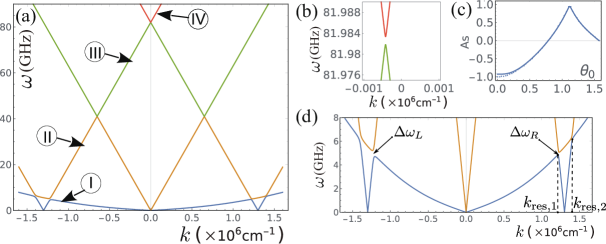
Figure 2: (color online) (a) Spectrum of magnetoelastic waves in the conical phase for $\theta_{0}=\pi/5$ showing four magnetoelastic bands originating from one helimagnon mode and tree acoustic modes – longitudinal, and left/right-polarized transverse modes. Different energy bands are highlighted by colors. Note a gap opening between each pair of adjacent bands. b) Magnified image of a gap opening between III and IV bands shifted from $k=0$ point. c) Band-gap asymmetry, $As=\left(\Delta\omega_{R}-\Delta\omega_{L}\right)/\left(\Delta\omega_{R}+\Delta\omega_{L}\right)$, between the left ($\Delta\omega_{L}$) and right ($\Delta\omega_{R}$) gap values centered near $-k_{\mathrm{res},1}$ and $k_{\mathrm{res},1}$ for the hybridized low-energy bands I and II as a function of $\theta_{0}$. d) Low energy sector of the spectrum showing a detailed picture of hybridization between I and II bands.

Let us discuss the magnetoelastic resonance between I and II bands. The momentum points of the first resonance in the vicinity of $\pm q$ (see Fig. 2 (d)) are resulted from the equations

$$v_{t}^{2}\left(k_{\text{res}}\pm q\right)^{2}=\left(\gamma JM_{0}\right)^{2}k_{\text{res}}^{2}\left(k_{\text{res}}^{2}+q^{2}\sin^{2}\theta_{0}\right).$$ (24)

By using the values $\gamma=2\pi g\times 1.4\,\text{MHz}\cdot\text{Gs}^{-1}$ ($g=2$), $q=-0.13\times 10^{7}\text{cm}^{-1}$, that corresponds to the period 48 nm, $M_{0}=1649$ Gs, and $JM_{0}^{2}\sim k_{B}T_{c}/a_{||}=0.26\times 10^{-6}$ erg/cm, where $T_{c}=127$ K is the Curie-Weiss temperature and $a_{||}=6.847\mathring{A}$ is the nearest Cr-Cr distance along the $z$-axis in CrNb₃S₆,Mandrus2013 one may find that the pair of resonance points are given by $k_{\text{res},1}=0.12\cdot 10^{7}\text{cm}^{-1}$ and $k_{\text{res},2}=0.14\cdot 10^{7}\text{cm}^{-1}$, where we suppose $\theta_{0}=\pi/2$. Then the resonance frequency $\omega_{\text{res}}=\sqrt{c_{44}/\rho}\left|k_{\text{res}}+q\right|$ takes the values 5.93 GHz and 7.59 GHz at these points, respectively.

IV.1.2 Band-gap asymmetry in the conical phase

As anticipated, there is the asymmetry between the left and right gap values, $\Delta\omega_{L}$ and $\Delta\omega_{R}$, centered near $-k_{\text{res}}$ and $k_{\text{res}}$, respectively, which occurs due to broken parity symmetry along the $z$ axis in the conical phase. Taking the notation for the left-hand side of Eq.(20) as $f(\omega)$, the gap in the resonant point of the frequency $\omega_{\text{res}}$ may be evaluated

$$\Delta\omega=2\left\{\left[\frac{f^{{}^{\prime}}(\omega_{\text{res}})}{f^{{}^{\prime\prime}}(\omega_{\text{res}})}\right]^{2}-2\frac{f(\omega_{\text{res}})}{f^{{}^{\prime\prime}}(\omega_{\text{res}})}\right\}^{\frac{1}{2}}.$$ (25)

The asymmetry between the gaps, defined as $As=\left(\Delta\omega_{R}-\Delta\omega_{L}\right)/\left(\Delta\omega_{R}+\Delta\omega_{L}\right)$ calculated both numerically and with the aid of the formula (25) is shown in Fig. 2 (c). It is clear that with decreasing $\theta_{0}$ the asymmetry gradually increases to some maximum value around $\theta_{0}=\pi/3$ and drops down afterwards to the minimum value at zero that corresponds to the forced ferromagnetic state. Mathematically, the asymmetry in the conical phase results from the $k$-linear term in (20). It includes the factor $\cos\theta_{0}\cos 2\theta_{0}$ that reaches the maximum absolute value at $\theta_{0}=0$ and $\cos^{-1}\left(1/\sqrt{6}\right)$, and zero at $\pi/4$ and $\pi/2$. This fact explains the absence of the asymmetry at the last particular points. The symmetry breaking of the dispersion spectrum admits non-reciprocal elastic wave propagation controlled by the external magnetic field directed along the chiral axis.

It should be emphasized that the asymmetry indicates involvement of elastic waves of different polarizations in the hybridization. To illustrate this fact, let us, at first, have a look at the well known result for the forced ferromagnetic phase, where only left-polarized transverse acoustic wave ($s_{-}\neq 0$), propagating along the magnetic ordering direction, is hybridized to the magnon bandAkhiezer1968 . This fact is a direct consequence of the rotations symmetry along the magnetization direction, which makes polarization of the wave a good quantum number. Since ferromagnetic magnons are only left-polarized, they are able to couple only to the sound wave that matches their handedness.

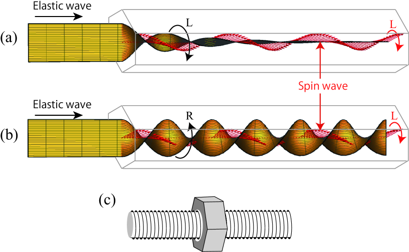
Figure 3: (color online) (a) When linearly polarized elastic wave is injected into the forced-ferromagnetic state along the chiral axis, it is decomposed into left- and right-handed circularly polarized waves. Then only either of them can resonantly hybridize with the spin wave which has the definite helicity due to the DM interaction and consequently attenuates. (b) The circularly polarized elastic wave with the chirality opposite to the spin wave can penetrate without attenuation. (c) Mechanical bolt-but analogue of the effect. The screw bolt and the nut correspond to the spin-wave and circularly polarized elastic wave. The nut can couple (hybridize) only when the chirality of the bolt matches the chirality of the nut. This situation is an analogue of the case shown in (a).

In Fig. 3, we schematically depict how the left-polarized acoustic wave selectively hybridize the spin wave in non-reciprocal manner, when the linearly polarized elastic wave is injected into the forced-ferromagnetic state along the chiral axis. In (a) we show that only either of left- or right-handed circularly polarized counterpart can hybridize with the spin wave which has the definite helicity due to the DM interaction. In this case, the corresponding counterpart attenuates. On the other hand, as in Fig. 3 (b) the circularly polarized elastic wave with the chirality opposite to the spin wave can penetrate without attenuation. This mechanism may be captured through “chiral bolt-nut”analogue as shown in Fig. 3 (c). In the case of conical phase with $\theta_{0}\neq\pi/2$, left- and right-handed spin waves are mixed and consequently, the linearly polarized elastic wave are decomopsed into left- and right-handed circularly polarized counterparts depending on the magnitude of $\theta_{0}$.

The same argument is applicable to the conical phase at $H^{z}=H_{c}^{z}$ ($\theta_{0}=0$) where rotation symmetry is restored, see Fig. 4. However, for $H^{z}<H_{c}^{z}$ the finite component of the magnetization appears perpendicular to the chiral axis, which breaks the rotation symmetry giving rise to the direct hybridization between right-polarized ($s_{+}\neq 0$) acoustic band and the helimagnon band. Therefore, the asymmetry factor, $As$, can be related to the difference between the contributions from the left- and right-polarized acoustic waves to the hybridization.

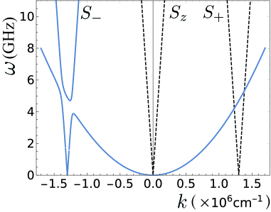
Figure 4: Spectrum of magnetoelastic waves at $\theta_{0}=0$, where the conical phase collapses to the forced ferromagnetic phase, calculated in the two-wave approximation (see Eq. (26)), which merges perfectly with the exact result given by Eq. (20). The dashed lines show the longitudinal and right-polarized acoustic waves decoupled from magnetic excitations. The band gap on the left hand side shows remaining hybridization between the parabolic ferromagnetic magnon spectrum and left-polarized acoustic wave.

To summarize this section, we would like to note that the measurements of the band gaps in the spectrum of magnetoelastic excitations can be useful for experimental estimation of magnetoelastic constants. As an example, we demonstrate how the constant $b_{44}$ responsible for hybridization between I and II bands may be determined from the experimental value for the band gap at $\theta_{0}=0$ of the phase transition from the conical phase to the induced ferromagnetic phase (see Fig. 4).

The choice of this specific point is motivated by the absence of contribution of another magnetoelastic constants to the gap value. For illustration, we restrict our analysis by two-wave approximation,two-wave where coupling of the amplitudes $\tilde{s}_{-}(k)$, $\delta\varphi(k)$ and $\delta\theta(k)$ is only retained in the vicinity of the momentum $q$. Then the frequencies may be found from determinant of the matrix

$$\left(\begin{array}[c]{ccc}\omega^{2}-v^{2}_{t}(k-q)^{2}&\beta_{1}(k-q)&i\beta_{1}(k-q)\\ \frac{1}{2}\beta_{2}(k-q)&-\varepsilon_{1k}&i\omega\\ \frac{i}{2}\beta_{2}(k-q)&i\omega&\varepsilon_{2k}\end{array}\right).$$ (26)

It can be observed from Eqs.(21,22) that

$$\varepsilon_{1k}=\varepsilon_{2k}=\gamma JM_{0}k^{2}+\frac{\beta_{1}\beta_{2}}{v^{2}_{t}},$$ (27)

and, as a consequence, only the constant $b_{44}$ controls interaction between the magnetic and the elastic subsystems.

Straightforward calculation results in the dispersion relation (see Fig. 4)

$$\left(\omega^{2}-v^{2}_{t}(k-q)^{2}\right)\left(\omega-\gamma JM_{0}k^{2}\right)=\beta_{1}\beta_{2}\frac{\omega^{2}}{v^{2}_{t}}.$$ (28)

By adapting the resonance condition in Eq. (24) and using the expansion $\omega=\omega_{0}+\delta\omega$, where $\omega_{0}=\gamma JM_{0}k^{2}_{\text{res}}$ is the frequency of the resonance, we find eventually the gap value

$$\delta\omega\approx\gamma M^{2}_{0}b_{44}\sqrt{\frac{Jk_{\text{res}}^{2}}{2c_{44}}}.$$ (29)

Consequently, the non-transmission band in the spectrum of the coupled oscillations enables a convenient way to find the magnetoelastic constant $b_{44}$ associated with torsion deformations around the $z$-axis.

IV.2 Soliton lattice phase

In this section, we consider the case when the static magnetic field is applied perpendicular to the chiral axis. For $H^{x}<H_{c}^{x}$, the magnetic chiral soliton lattice phase is realized, which is characterized by the following spatial dependence of the equilibrium background magnetization, $M_{0\pm}(z)=M_{0}e^{\pm i\varphi_{0}(z)}$, and $M_{0z}=0$, where $\varphi_{0}(z)$ is given by Eq. (7). At $H^{x}=0$, the Taylor series of $\varphi_{0}$ have only one term, $qz$, which corresponds the simple spiral with one harmonic. For any nonzero $H^{x}$, Jacobi’s amplitude function in $\varphi_{0}(z)$ has nontrivial power series giving origin to the multiharmonic nature of the resulting soliton lattice.

In order to obtain the spectrum of magnetoelastic excitations for the soliton lattice phase, we expand the total magnetization up to the linear order in fluctuations, $\delta m_{\pm}(z,t)=\pm iM_{0}e^{\pm i\varphi_{0}(z)}\delta\varphi(z,t)$ and $\delta m_{z}(z,t)=-M_{0}\delta\theta(z,t)$. The dynamical equations can be found straightforwardly from Eq. (5, 6) by linearizing them in $\delta\varphi$ and $\delta\theta$, which gives the following expressions after some algebra

$$\frac{\partial^{2}s_{\pm}}{\partial t^{2}} =v^{2}_{t}\frac{\partial^{2}s_{\pm}}{\partial z^{2}}-\beta_{1}\frac{\partial}{\partial z}\left(e^{\pm i\varphi_{0}}\delta\theta\right),$$ (30)

$$\frac{\partial\delta\theta}{\partial t} =-JM_{0}\gamma\operatorname{\hat{\mathcal{L}}}\delta\varphi,$$ (31)

$$\frac{\partial\delta\varphi}{\partial t} =JM_{0}\gamma\left[\operatorname{\hat{\mathcal{L}}}-\left(\frac{d\varphi_{0}}{dz}-q\right)^{2}\right]\delta\theta+\gamma f\left(\frac{\pi}{2}\right)\delta\theta$$

$$-\frac{\beta_{2}}{2}\left(e^{-i\varphi_{0}}\frac{\partial s_{+}}{\partial z}+e^{i\varphi_{0}}\frac{\partial s_{-}}{\partial z}\right),$$ (32)

where $\operatorname{\hat{\mathcal{L}}}=-\partial_{z}^{2}+m^{2}\cos\varphi_{0}$ denotes the Lamé operator, and the sine-Gordon equation, providing the phase modulation in the soliton lattice, $\partial^{2}_{z}\varphi_{0}=m^{2}\sin\varphi_{0}$, was accounted for. The equation of motion for $s_{z}$ is totally decoupled from these equations and corresponds to the acoustic band with the trivial dispersion relation $\omega=v_{l}k$.

It is natural to assume that some generalized Fourier series for $s_{\pm}$, $\delta\theta$, and $\delta\varphi$ in terms of the Lamé operator’s eigenfunction can provide the solution of the eigenvalue problem when the magnetoelastic coupling is fairly small. However, in realizing this approach one faces with a problem, since it turns out that, in practice, it is not possible to treat this infinite series as being explicitly controlled by any small parameter whatsoever.

To tackle this problem, let us note the case for the conical phase, where the gauge transformation for $s_{\pm}$ was applied to remove the periodic terms in the equations of motion, which appeared owing to the basic harmonics, $\sin\theta_{0}e^{\pm iqz}$, of the underlying magnetic structure. Unfortunately, this special trick cannot be directly implemented for Eqs. (30)-(32) because of the multi-harmonic character of the soliton lattice phase. Nevertheless, we found that the expansion of the periodic terms with respect to the small parameter $\kappa^{2}$, which is controlled by $H^{x}$, with subsequent Fourier transformation of the dynamical equations turns out to be effective.

Indeed, the coefficients on the right hand side of Eqs. (30)–(32) can be expanded in power series of $\kappa$

$$\cos\varphi_{0} =\frac{\kappa^{2}}{8}-\cos qz-\frac{\kappa^{2}}{8}\cos 2qz+\mathcal{O}(\kappa^{4}),$$ (33)

$$e^{\pm i\varphi_{0}} =\frac{\kappa^{2}}{8}-e^{\pm iqz}-\frac{\kappa^{2}}{8}e^{\pm 2iqz}+\mathcal{O}(\kappa^{4}),$$ (34)

$$\frac{d\varphi_{0}}{dz} =q+\frac{\kappa^{2}}{4}q\cos qz+\mathcal{O}(\kappa^{4})$$ (35)

where $\kappa$ is determined by applied magnetic field.

One particular advantage of the present formulation is evident for small and intermediate magnetic fields, when $H^{x}$ is far below $H_{c}^{x}$; because these expansions involve the small factor $\kappa^{2}$, the series can be terminated at low order. The method is also sufficiently simple algebraically to enable us to obtain a magnetoelastic spectrum in the soliton lattice phase with a given accuracy.

Inserting the expansions (33)-(35) into the system (30) -(32) and holding terms up to the $\kappa^{2}$ order, we get

$$\left(\omega^{2}-v_{t}^{2}k^{2}\right)s_{\pm}(k,\omega) =ik\beta_{1}\left[\frac{\kappa^{2}}{8}\delta\theta(k,\omega)-\delta\theta(k\mp q,\omega)-\frac{\kappa^{2}}{8}\delta\theta(k\mp 2q,\omega)\right],$$ (36)

$$-i\omega\delta\theta(k,\omega) =-JM_{0}\gamma k^{2}\left[\delta\varphi(k,\omega)-\frac{q^{2}\kappa^{2}}{8k^{2}}\left(\delta\varphi(k+q,\omega)+\delta\varphi(k-q,\omega)\right)\right],$$ (37)

$$-i\omega\delta\varphi(k,\omega) =JM_{0}\gamma k^{2}\left[\delta\theta(k,\omega)-\frac{q^{2}\kappa^{2}}{8k^{2}}\left(\delta\theta(k+q,\omega)+\delta\theta(k-q,\omega)\right)\right]+\gamma f\left(\frac{\pi}{2}\right)\delta\theta(k,\omega)$$

$$-\frac{i\beta_{2}\kappa^{2}}{16}\left[ks_{+}(k,\omega)+ks_{-}(k,\omega)-(k+2q)s_{+}(k+2q,\omega)-(k-2q)s_{-}(k-2q,\omega)\right]$$

$$+\frac{i\beta_{2}}{2}\left[(k+q)s_{+}(k+q,\omega)+(k-q)s_{-}(k-q,\omega)\right].$$ (38)

To obtain a closed set of dynamical equations, we supplemented Eqs. (36)–(38) by similar equations of motion for higher order harmonic amplitudes keeping only the terms with $k\pm q$ and $k\pm 2q$. The resulting set of twenty coupled equations was solved numerically to obtain magnetoelastic band structure shown in Fig. 5.

The resulting band structure in Fig. 5 can be qualitatively understood if we note that the periodic nature of the magnetic soliton lattice gives origin to the magnetic Brillouin zone determined by the soliton lattice period and controlled by external magnetic field. Magnetic excitation can directly feel this periodic background which naturally results into the helimagnon Bloch bands, where different branches are separated from each other due to the Bragg’s reflection from periodic potential of the underlying magnetic superlattice. These helimagnon Bloch bands hybridize with acoustic bands due to the magnetoelastic coupling resulting into the energy spectrum shown in Fig. 5 (b).

To gain further insight concerning the excitation spectrum, it may be useful to decompose the background magnetization of the soliton lattice into the harmonic series KO2015

$$\frac{M_{x0}}{M_{0}} =\frac{2(K-E)}{\kappa^{2}K}-1-\frac{\pi^{2}}{\kappa^{2}K^{2}}\sum_{n\not=0}\frac{ne^{inGz}}{\sinh\left(n\pi\frac{K^{\prime}}{K}\right)},$$ (39)

$$\frac{M_{y0}}{M_{0}} =\frac{i\pi^{2}}{\kappa^{2}K^{2}}\sum_{n}\frac{ne^{inGz}}{\cosh\left(n\pi\frac{K^{\prime}}{K}\right)},$$ (40)

where

$$G=\pi^{2}q/(4KE)=q\left[1-\frac{\kappa^{4}}{32}+\mathcal{O}\left(\kappa^{6}\right)\right]$$ (41)

is the wave vector of the soliton lattice, and $K$ ($K^{\prime}$) denotes the first order elliptic integral with the modulus $\kappa$ ($\kappa^{\prime 2})^{1/2}$). In contrast to the conical phase, the additional contributions $e^{inGz}$, $|n|\geq 2$, appear in the spatial distribution of the nonuniform magnetic background along with the basic ones, $e^{\pm iGz}$.

Inspection of Fig. 5 (a) indicates that we can assign different coordinate systems related to each harmonic, where the points $nq$ are used as the coordinate system origin, and, as a consequence, the excitation branches of the elastic excitations are replicated. Similarly to the simple spiral, the resonance at $k_{\text{res},\alpha}$ ($\alpha=1,2$) points near the $nq$ values occurs, which is determined by the following condition

$$v^{2}_{t}\left(k_{\text{res},\alpha}\pm nq\right)^{2}=\varepsilon_{1k}\varepsilon_{2k}$$ (42)

giving resonant frequencies $\omega^{(n)}_{\text{res},\alpha}=\sqrt{c_{44}/\rho}|k_{\text{res},\alpha}\pm nq|$. By neglecting the magnetoelastic contributions to the energies $\varepsilon_{1k,2k}$, we recover the result of Eq. (24).

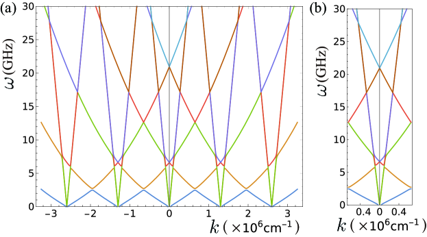
Figure 5: (color online)Spectrum of magnetoelastic waves in the soliton lattice phase in the extended (a) and reduced (b) zone schemes. The colors indicate different excitation bands separated from each other by hybridization gaps.

Proceeding similarly to the analysis of the conical phase, one may observe that the first gap in the excitation spectrum in the vicinity of $k=q$ originates from hybridization of the amplitudes $s_{-}(k-q)$, $\delta\theta(k)$ and $\delta\varphi(k)$. The system (36,37,38) lends support to the coupling

$$\left[\omega^{2}\!-v^{2}_{t}(k-q)^{2}\right]\!s_{-}(k-q)+i\beta_{1}(k-q)\delta\theta(k)=0,$$ (43)

$$i\omega\delta\theta(k)-\varepsilon_{1k}\delta\varphi(k)=0,$$ (44)

$$i\omega\delta\varphi(k)+\varepsilon_{2k}\delta\theta(k)+\frac{i\beta_{2}}{2}(k-q)s_{-}(k-q)=0$$ (45)

which brings about the result for the first hybridization gap between the magnetic and acoustic band

$$\left.\Delta\omega\right|_{k=q}\approx\gamma M^{2}_{0}b_{44}\sqrt{\frac{Jq^{2}}{2c_{44}}}.$$ (46)

The extension of this approach to calculation of the second order gap seems obvious. Apparently, keeping only the amplitudes $s_{-}(k-2q)$, $\delta\theta(k)$ and $\delta\varphi(k)$ in Eqs (36)–(38), one finds the gap near the resonant point $k=2q$

$$\left.\Delta\omega\right|_{k=2q}\approx\gamma M^{2}_{0}b_{44}\frac{\kappa^{2}}{4}\sqrt{\frac{Jq^{2}}{2c_{44}}}=\frac{\kappa^{2}}{4}\left.\Delta\omega\right|_{k=q}.$$ (47)

It may be further proved that the width of the $n$-th gap decreases exponentially, $\left.\Delta\omega\right|_{k=nq}\sim\kappa^{2n-2}$, similar to the result for spin-wave spectrum of the relativistic spiral Izyumov1987 .

Apart from hybridization between the spin and elastic waves, there is a pure magnetic band gap originating from the Bragg’s reflection of the helimagnons from the periodic potential of the soliton lattice. It can be regarded as the splitting $\Delta\omega_{\rm{sp}}=a^{3}M_{0}H^{x}/(2\hbar)$ between the acoustic and optic branches of spin fluctuations at the boundary of the magnetic Brillouine zone KO2015 , which is visible in Fig. 5 (a) as lifted degeneracies at the points $nG/2\approx nq/2$. In contrast to Eq. (46), the magnetic gap is directly controlled by the magnetic field rather than a strength of the magnetoelastic coupling.

V Discussions

A salient peculiarity of the conical phase is the conspicuous asymmetry between the left and right band-gaps in the spectrum of the coupled magnetoelastic waves. In practice, it is the phonon mode that of major importance after hybridization, because the elastic stiffness is measured experimentally at different external magnetic fields as the ultrasonic response. The tunable non-reciprocity governed by the magnetic field is potentially applicable in the construction of ultrasound devices using chiral helimagnets.

In contrast to the conical magnetic structure, time-reversal symmetry for elastic wave propagation is kept for the soliton lattice and for the simple spiral, particularly. Another notable difference in comparison with the conical phase, the magnetoelastic resonance in the soliton lattice has the multi-resonance behavior. This result confirms the intuitive expectation that the resonance occurs whenever the wave vector of a spreading elastic wave matches a modulation of the non-uniform magnetic background. In contrast to the conical magnetic structure, the soliton lattice consists of higher-order harmonics indexed by integer, and each of the components contributes to the resonance separately. We emphasize that an assessment of the hybridization constant $b_{44}$ at the point, where the conical phase is collapsed in favor of the forced ferromagnetic phase, may successfully be combined with measurements of multiresonance ultrasound absorption in the soliton lattice. The scheme provides a promising tool for an experimental probe of the soliton lattice phase. Regarding potential applications of the theory, it is useful to highlight that while lattice and elastic properties of MnSi and related compounds are well known Lamago2010 ; Petrova2011 , there remains a considerable need for experimental information on the phonon dispersion and the phonon density of states in CrNb₃S₆.

While our treatment is designed for crystals of hexagonal symmetry it nonetheless provides the framework for studies of magnetoelastic effects in chiral helimagnets of other crystal classes. For example, the tetragonal insulating materials CuB₂O₄ Roessli2001 and Ba₂CuGe₂O₇ Zheludev1998 , the trigonal metallic compound Yb(Ni_1-xCu_x)₃Al₉ Matsumura2017 may be named, where ample evidences for the formation of a chiral magnetic soliton lattice state, an anticipated outcome of a monoaxial chiral helimagnet, were reported.

Some limitations of our analysis should be mentioned. In the equilibrium configuration $\boldsymbol{M}_{0}$, the magnetoelastic terms were discarded. These effects may be described by the double sine-Gordon model, also known as the sine-Gordon model with crystalline anisotropy of the second order Izyumov1984 . This specific issue will be addressed in future work. Here, it is worth noting that the enhanced anisotropic change in shape both for skyrmion lattice and individual skyrmions was revealed in FeGe by Lorentz transmission electron microscopy under uniaxial tensile stress deformation. It was ascribed to the strain-induced anisotropic modulation of DM interaction Shibata2015 . On the contrary, the stress-driven topological phase transition in MnSi from the skyrmion lattice phase to the conical phase was interpreted by strain-induced magnetic anisotropy on the basis of the Ginzburg-Landau phenomenology with an account of magnetoelastic contribution to the free energy Nii2015 .

Another difficulty of possible application of the work may arise owing to the magneto-elastic correlations in CrNb₃S₆ Mito2015 . The diffuse scattering measurements of the crystal structure of CrNb₃S₆ demonstrate that there is a bias towards a disorder in the Cr sublattice Chernyshov2015 . It is suggesting that the disorder occurs due to clustering of Cr ions in hexagonal fragments within the layers. It was found that such a specific correlated disorder strongly affects the magnetic ordering temperature. A follow up work designed to evaluate an interplay between the correlated disorder and magnetic properties would be useful.

Measurements on thin films of CrNb₃S₆ showed that the chiral soliton lattice exhibits interesting phenomena due to confinement from the presence of magnetic domains extended for approximately 1 $\mu$m in helix direction Togawa2015 ; Wang2017 . An important question for future studies is to determine an effect of the domain structure on the ultrasound wave propagation. We believe that our theoretical analysis may serve as an appropriate starting point to touch on these issues.

VI Conclusions

In summary, we have investigated the spectrum of coupled magnetoelastic waves propagating along the helicoidal axis in crystals of hexagonal symmetry having spiral magnetic order due to DM interaction. Based on the example of spin and elastic waves we elucidate how torsion deformations are related with spin chirality. We clarified peculiar nature of magnetoelastic resonance for particular phases of the monoaxial chiral axis: the conical phase and the soliton lattice phase. To the best of our knowledge, an effect of magnetoelastic coupling for the latter one has not been studied before.

So far some kinds of multiresonance phenomena associated with the soliton lattice have been predicted, including an appearance of higher-order satellites in the neutron diffraction patterns Izyumov1984 ; KO2015 , a spike-like behavior of magnetoresistance originated from scattering of electrons by the magnetic superlattice by the chiral solitons KPO2011 ; Okamura2018 , and multiple spin resonance of the chiral soliton lattice KO2009 . We expect the present study on magneto-elastic coupling may expand the scope of these multi-resonance or scattering phenomena. In particular, we show that the non-reciprocal spin wave around the forced-ferromagnetic state has potential capability to convert the linearly polarized elastic wave to circularly polarized one with the chirality (helicity) opposite to the spin wave chirality.

- (1) E. Fawcett, J.P. Maita and J.H. Wernick, Int. J. Magn. 1, 29 (1970).
- (2) M. Matsunaga, Y. Ishikawa and T. Nakajima, J. Phys. Soc. Japan 51, 1153 (1982).
- (3) G.A. Valkovskiy, E.V. Altynbaev, M.D. Kuchugura, E.G. Yashina, A.S. Sukhanov, V.A. Dyadkin, A.V. Tsvyashchenko, V.A. Sidorov, L.N. Fomicheva, E. Bykova, S.V. Ovsyannikov, D.Yu. Chernyshov and S.V. Grigoriev, J. Phys.: Condens. Matter 28, 375401 (2016).
- (4) O. L. Makarova, A. V. Tsvyashchenko, G. Andre, F. Porcher, L. N. Fomicheva, N. Rey, and I. Mirebeau, Phys. Rev. B 85, 205205 (2012).
- (5) V. Dyadkin, S. Grigoriev, S.V. Ovsyannikov, E. Bykova, L. Dubrovinsky, A. Tsvyashchenko, L.N. Fomicheva, and D. Chernyshov, Acta Crystallogr. B Struct. Sci. Cryst. Eng. Mater. 70 676, (2014).
- (6) N. Martin, M. Deutsch, J.P. Itié, J.-P. Rueff, U.K. Rössler, K. Koepernik, L.N. Fomicheva, A.V. Tsvyashchenko, and I. Mirebeau, Phys. Rev. B 93, 214404 (2016).
- (7) M.L. Plumer and M.B. Walker, J. Phys. C: Solid State Phys. 15, 7181 (1982).
- (8) M.L. Plumer, J. Phys. C: Solid State Phys. 17, 4663 (1984).
- (9) S.V. Maleyev, J. Phys.: Condens. Matter 21, 146001 (2009).
- (10) A.E. Petrova, S.M. Stishov, J. Phys.: Condens. Matter 21, 1960001 (2009).
- (11) A.E. Petrova, S.M. Stishov, Phys. Rev. B 91, 214402 (2016).
- (12) Y. Togawa, T. Koyama, K. Takayanagi, S. Mori, Y. Kousaka, J. Akimitsu, S. Nishihara, K. Inoue, A. S. Ovchinnikov, and J. Kishine, Phys. Rev. Lett. 108, 107202 (2012).
- (13) S. Mühlbauer, B. Binz, F. Jonietz, C. Pfleiderer, A. Rosch, A. Neubauer, R. Georgii, and P. Böni, Science 323, 915 (2009).
- (14) X. Z. Yu, Y. Onose, N. Kanazawa, J. H. Park, J. H. Han, Y. Matsui, N. Nagaosa, and Y. Tokura, Nature (London) 465, 901 (2010).
- (15) W. Münzer, A. Neubauer, T. Adams, S. Mühlbauer, C. Franz, F. Jonietz, R. Georgii, P. Böni, B. Pedersen, M. Schmidt, A. Rosch, and C. Pfleiderer, Phys. Rev. B 81, 041203(R) (2010).
- (16) S. Seki, X. Z. Yu, S. Ishiwata, and Y. Tokura, Science 336, 198 (2012).
- (17) Y. Nii, T. Nakajima1, A. Kikkawa, Y. Yamasaki, K. Ohishi, J. Suzuki, Y. Taguchi, T. Arima, Y. Tokura and Y. Iwasa, Nat.Commun. 6, 8539 (2015).
- (18) C. Kittel, Phys. Rev. 110, 836 (1958).
- (19) V.G. Bar’yahtar and E.P. Stefanovski, Fiz. Tverd. Tela 11, 1946 (1969).
- (20) K.B. Vlasov, V.G. Bar’yahtar and E.P. Stefanovski, Fiz. Tverd. Tela 15, 3656 (1973).
- (21) E.A. Turov and V.G. Shavrov, Sov. Phys. Usp. 26, 593 (1983).
- (22) V.D. Buchel’nikov, V.G. Shavrov, Sov. Phys. Solid State 31, 23 (1989).
- (23) V.D. Buchel’nikov, I.V. Bychkov and V.G. Shavrov, Fiz. Met. Metalloved. 11, 12 (1990).
- (24) C. Vittoria, Phys. Rev. B 92, 064407 (2015).
- (25) Y. Iguchi, S. Uemura, K. Ueno, Y. Onose, Phys. Rev. B 92 (2015)184419.
- (26) S. Seki, Y. Okamura, K. Kondou, K. Shibata, M. Kubota, R. Takagi, F. Kagawa, M. Kawasaki, G. Tatara, Y. Otani, and Y. Tokura, Phys. Rev. B 93, 235131 (2016).
- (27) X.-X. Zhang and N. Nagaosa, New J. Phys. 19, 043012 (2017).
- (28) N. Kanazawa, Y. Nii, X.-X. Zhang, A.S. Mishchenko, G. De Filippis, F. Kagawa, Y. Iwasa, N. Nagaosa and Y. Tokura, Nat.Commun. 7, 11622 (2016).
- (29) Y. Hu and B. Wang, New J. Phys. 19, 123002 (2017).
- (30) A. Rosch, Nat. Mater. 15, 1231 (2016).
- (31) V.D. Buchel’nikov, I.V. Bychkov and V.G. Shavrov, J. Magn. Magn. Mater. 118, 169 (1993).
- (32) W.P. Mason, Phys. Rev. 96, 302 (1954).
- (33) R.L. Comstock and B.A. Auld, J. Appl. Phys. 34, 1461 (1963).
- (34) N.J. Ghimire, M.A. McGuire, D.S. Parker, B. Sipos, S. Tang, J.-Q. Yan, B.C. Sales, and D. Mandrus, Phys. Rev. B 87, 104403 (2013).
- (35) R. Gaillac, P. Pullumbi and F.-X. Coudert, J. Phys. Condens. Matter 28, 275201 (2016).
- (36) A. I. Akhiezer, V. G. Baryakhtar, and S. V. Peletminskii, in Spin Waves, edited by S. Doniach (North-Holland Publishing Co., Amsterdam, 1968).
- (37) Two-wave approximation used here is analogous to the case of magnetic resonance problem. See, for example, C. P. Slichter, “Principles of Magnetic Resonance,”(Springer, 1990). The role of AC magnetic field in the magnetic resonance problem is played by the elastic wave in the present case.
- (38) P.H. Higgs, Phys. Lett. 12, 132 (1964).
- (39) V.D. Buchel’nikov, I.V. Bychkov, V.G. Shavrov, JETP 78, 398 (1994).
- (40) D. Chandrasekharaiah and L. Debnath, Continuum Mechanics (Academic Press, San Diego, 1994).
- (41) V.I. Fedorov, A.G. Gukasov, V. Kozlov, S.V. Maleyev, V.P. Plakhty, I.A. Zobkalo, Phys. Lett. A 224, 372 (1997).
- (42) S. V. Grigoriev, D. Chernyshov, V. A. Dyadkin, V. Dmitriev, S. V. Maleyev, E. V. Moskvin, D. Menzel, J. Schoenes, and H. Eckerlebe, Phys. Rev. Lett. 102, 037204 (2009).
- (43) S.V. Grigoriev, D. Chernyshov, V.A. Dyadkin, V. Dmitriev, E.V. Moskvin, D. Lamago, Th. Wolf, D. Menzel, J. Schoenes, S.V. Maleyev, and H. Eckerlebe, Phys. Rev. B 81, 012408 (2010).
- (44) J. Kishine and A. S. Ovchinnikov, Solid State Phys. 66, 1 (2015).
- (45) Yu.A. Izyumov, Diffraction of Neutrons on Long-Periodic Structures [in Russian] (Energoatomizdat, Moscow, 1987).
- (46) D. Lamago, E. S. Clementyev, A. S. Ivanov, R. Heid, J.-M. Mignot, A. E. Petrova, and P. A. Alekseev, Phys. Rev. B 82, 144307 (2010).
- (47) A.E. Petrova, V.N. Krasnorussky, W.M. Yuhasz, T.A. Lograsso and S.M. Stishov, J. Phys.: Conf. Ser. 273, 012056 (2011).
- (48) Y.A. Izyumov, Sov. Phys. Usp. 27, 845 (1984).
- (49) J. Kishine, I. V. Proskurin, and A. S. Ovchinnikov, Phys. Rev. Lett. 107, 017205 (2011).
- (50) S. Okamura, Y. Kato and Y. Motome, J. Phys. Soc. Jpn (in press).
- (51) J. Kishine and A. S. Ovchinnikov, Phys. Rev. B 79, 220405(R) (2009).
- (52) B. Roessli, J. Shefer, G.A. Petrakovskii, B. Ouladdiaf, M. Boehm, U. Staub, A. Vorotinov, L. Bezmaternikh, Phys. Rev. Lett. 86, 1885 (2001).
- (53) A. Zheludev, S. Maslov, G. Shirane, Y. Sasago, N. Koide and K. Uchinokura, Phys. Rev. B 57, 2968 (1998).
- (54) T. Matsumura, Y. Kita, Y. Yoshikawa, S. Michimura, T. Inami, Y.Kousaka, K. Inoue, and S. Ohara, J. Phys. Soc. Jpn. 86, 124702 (2017).
- (55) K. Shibata, J. Iwasaki, N. Kanazawa, S. Aizawa, T. Tanigaki, M. Shirai, T. Nakajima, M. Kubota, M. Kawasaki, H. S. Park, D. Shindo, N. Nagaosa and Y. Tokura, Nat. Nanotechnol. 10, 589 (2015).
- (56) M. Mito, T. Tajiri, K. Tsuruta, H. Deguchi, J. Kishine, K. Inoue, Y. Kousaka, Y. Nakao, and J. Akimitsu, J. Appl. Phys. 117, 183904 (2015).
- (57) V. Dyadkin, F. Mushenok, A. Bosak, D. Menzel, S. Grigoriev, P. Pattison, and D. Chernyshov, Phys. Rev. B 91, 184205 (2015).
- (58) Y. Togawa, T. Koyama, Y. Nishimori, Y. Matsumoto, S. McVitie, D. McGrouther, R. L. Stamps, Y. Kousaka, J. Akimitsu, S. Nishihara, K. Inoue, I.G. Bostrem, Vl. E. Sinitsyn, A.S. Ovchinnikov, and J. Kishine, Phys. Rev. B 92, 220412(R) (2015).
- (59) L. Wang, N. Chepiga, D.-K. Ki, L. Li, F. Li, W. Zhu, Y. Kato, O.S. Ovchinnikova, F. Mila, I. Martin, D. Mandrus, and A.F. Morpurgo, Phys. Rev. Lett. 118, 257203 (2017).