Triaxiality Inhibitors in N-Body Simulations

Abstract

Numerous previous studies have investigated the phenomenon wherein initially spherical N-body systems are distorted to triaxial shapes. We report on an investigation of a previously described orbital instability that should oppose triaxiality. After verifying the instability with numerical orbit integrations that extend the original analysis, we search for evidence of the instability in N-body systems that become triaxial. Our results highlight the difficulty in separating dynamical process from finite-N effects. While we argue that our analysis points to the presence of the instability in simulated triaxial systems, discreteness appears to play a role in mimicking the instability. This suggests that predicting the shapes of real-world systems, such as dark matter halos around galaxies, based on such simulations involves more uncertainty than previously thought.

1. Introduction

Elliptical galaxies, galactic bulges, and some star clusters are well-approximated by collisionless models. It is also commonly assumed that dark matter halos around galaxies are best described as collisionless systems. All of these systems commonly have triaxial shapes that are typically described in terms of semi-axis lengths labeled $a$, $b$, and $c$ for long, intermediate, and short axes, respectively. In particular, simulated dark matter halos that form via hierarchical growth in cold dark matter cosmologies are generally triaxial with mean axial ratios $b/a\sim 0.6$ and $c/a\sim 0.4$ (Bardeen et al., 1986; Barnes & Efstathiou, 1987; Frenk et al., 1988; Dubinski & Carlberg, 1991; Jing & Suto, 2002; Bailin & Steinmetz, 2005; Allgood et al., 2006).

Attempts to understand the development of this triaxiality typically invoke what has become known as the radial orbit instability (ROI) (e.g., Merritt & Aguilar, 1985; Bardeen et al., 1986; Palmer & Papaloizou, 1987). This instability starts with a spherical system that hosts particles on radial orbits. The radial anisotropy of the orbits may be prescribed by initial conditions or it may develop as a result of a dynamically cold collapse. Detailed comparisons of the onset and triggering of the ROI in these situations has been previously presented (Barnes, Lanzel, & Williams, 2009). Independent of the specifics of the initial conditions, the instability grows as neighboring orbits tend to become aligned along a direction that has slightly more particles than others. The end products of this instability are important as the shapes of simulated dark matter halos impact how they will interact with satellite objects (e.g., Shaya et al., 2010). At the same time, this instability also affects density profiles of simulated halos (Barnes et al., 2005; Bellovary et al., 2008). Both of these effects could have observable consequences, if real halos are accurately modeled by simulations.

Our goal in this work is to complement those earlier studies by investigating how simulated systems halt, and even reverse, their evolutions to triaxial shapes. In particular, we are interested in an orbit instability that arises in triaxial systems which deflects orbits that lie near principal planes. This type of instability has been considered previously (Binney, 1981; Merritt & Fridman, 1996), but Adams et al. (2007) have provided a more recent detailed analysis. What we refer to as the Adams instability acts to change orbits that support triaxial shapes. Particles that orbit near principal planes can show exponential divergence perpendicular to those planes. In this way, orbital families that would underlie a triaxial shape are depleted. We expect that a system vulnerable to the Adams instability would become more spherical or, at least, have a limited range of non-sphericity. The work in Adams et al. (2007) focuses on the behavior of orbits in the central region of a cusped potential. As we are interested in looking at the behavior of entire simulated systems, our work picks up a thread from theirs by extending the investigation to outer regions of triaxial, cuspy potentials.

The larger part of our investigation searches for evidence of the instability in N-body simulations. We use the publicly available GADGET-2 code (Springel, 2005) to evolve systems with $10^{5}\leq N\leq 10^{6}$ in cosmological and non-cosmological situations. The time dependence of the instability for orbits in smooth, analytical potentials forms a template to search for signs of the instability in N-body systems, however the discrete nature of these systems complicates our approach. A similar situation arises in recent investigations of isolated and initially cold systems which show that initially spherical systems with small-scale density fluctuations will evolve in a manner similar to systems with initial triaxiality (Benhaiem & Sylos Labini, 2015).

The remainder of the paper will lay out our methods and results. Section 2 details our extension of the Adams et al. (2007) work to include non-central regions of triaxial systems. Descriptions of the initial conditions and evolutions of our N-body models form § 3. Our investigation of the impact of discreteness effects follows in Section 4. We summarize the results of our search for evidence of the Adams instability in N-body simulations in § 5.

2. Adams Instability in Smooth Potentials

The Adams instability has been observed in triaxial potentials with the form

$$\Phi(x,y,z)=2\int_{0}^{\infty}\frac{\psi(m)\,du}{\sqrt{(a^{2}+u)(b^{2}+u)(c^{2}+u)}},$$ (1)

where $m$ is length defined by

$$m^{2}=\frac{x^{2}}{a^{2}}+\frac{y^{2}}{b^{2}}+\frac{z^{2}}{c^{2}}.$$ (2)

The values $a$, $b$, and $c$ specify the long, intermediate, and short semi-axis lengths of the triaxial shape. The $\psi$ function is defined as (Chandrasekhar, 1969; Binney & Tremaine, 1987)

$$\psi(m)=\int_{m}^{\infty}2m^{\prime}\,\rho(m^{\prime})\,dm^{\prime}.$$ (3)

The Adams et al. (2007) work uses two common analytical density profiles, (Hernquist, 1990; Navarro, Frenk, & White, 1996)

$$\rho_{NFW} = \frac{\rho_{0}}{m(1+m)^{2}}\quad\mbox{and}$$

$$\rho_{H} = \frac{\rho_{0}}{m(1+m)^{3}}.$$ (4)

As the precise form of the potential is not of interest here, we will concern ourselves only with the Navarro-Frenk-White (NFW) form and set $\rho_{0}=1$.

Analytical expressions for the potential and acceleration in the central regions of such density distributions have been derived (Poon & Merritt, 2001; Adams et al., 2007). Based on these expressions, one can focus on the behavior of accelerations for particles that approach the origin along one of the principal axes. For concreteness, we imagine a particle moving towards the center nearly along the long ($x$) axis with the particle’s $y$ and $z$ positions being $\ll 1$. With these conditions, the $x$-acceleration becomes a step function about the origin (Figure 1a). The acceleration is constant and negative for $x>0$ and immediately becomes positive (and constant) for $x<0$. The $y$- and $z$-accelerations do not change sign with $x$, but reach their largest magnitudes at $x=0$. A representative $y$-acceleration curve is shown in Figure 1b. These accelerations work to create a large change in the direction of the velocity vector perpendicular to the long axis as it passes near the origin. This seems to be the origin of the instability. It is absent for particles that do not move along principal axes because the accelerations take on very different characteristics in other regions. Figure 2 shows acceleration behaviors near $x=0$ when $z$ remains small, but $y$ does not. In this non-principal axis situation, the $x$-acceleration is nearly harmonic and the $y$-acceleration is nearly constant.

Figure 1.— The $x$ dependence of accelerations for a potential with $a=\sqrt{2}$, $b=1$, $c=0.5071$ along a path where $y=z=10^{-4}$. Panel a shows the $x$-component of the acceleration while panel b shows the $y$-component. The rapid change in sign of $x$-acceleration coupled with the more impulsive nature of the $y$-acceleration lead to strong deflections of particles moving along principal axes as they pass near the origin.

Figure 2.— The $x$ dependence of accelerations for a potential with $a=\sqrt{2}$, $b=1$, $c=0.5071$ along a path where $y=0.2$ and $z=10^{-4}$. Panel a shows the $x$-component of the acceleration while panel b shows the $y$-component. The step-like feature of the $x$-acceleration and the impulsive nature of the $y$-acceleration have been removed, guaranteeing that particle velocities do no undergo sudden changes.

We begin by validating our numerical orbit integration routines through comparisons with orbits highlighted in Adams et al. (2007). The integration scheme uses a standard variable time step, Runge-Kutta approach (Press et al., 1994). Using the analytical approximation to the potential near the center, we have found a good match to an orbit in Adams et al. (2007, their Figure 3). The close comparison of orbit shape and size, along with the instability behavior, between Figure 3 and similar figures in Adams et al. (2007) serve as evidence that we are seeing the same behavior using our techniques. With the success of this base step, we extend to a full NFW potential, not relying on the limiting, analytical forms. Figure 4 shows a comparison between long-axis potential values from the centrally-limited approximation (labeled ‘Analytic’) and the full NFW form (labeled ‘Grid’). In extending beyond the central region, Equation 1 has been numerically evaluated to determine potential values on a three-dimensional grid with logarithmic spacing. Similarly, expressions for accelerations have been analytically determined by differentiating Equation 1. The resulting integrals have then been numerically evaluated on the same grid as the potentials. The logarithmic grid allows for better spatial resolution near the center of the potential where more dramatic changes in potential and acceleration occur. Spline interpolation routines are used to determine values at arbitrary locations in the grid. We utilize the EZSPLINE implementation of the PSPLINE library, http://w3.pppl.gov/ntcc/PSPLINE/. In regions where orbits are investigated, analytical and grid-based values of potential vary by as much as 15%. Accelerations are calculated on the same grid by numerically integrating spatial derivatives of Equation 1. With these values, our integrations conserve energy to roughly one part in one thousand over roughly 100 orbits.

Figure 3.— Panel a shows a projection of a particle orbit that originates near the $x-z$ plane, with initial $y=10^{-8}$ and undergoes exponential growth in a potential with $a=\sqrt{2}$, $b=1$, $c=0.5071$. This shape should be compared to the orbit in Figure 3 of Adams et al. (2007). Panel b shows how the $y$ position of the orbit grows with time, replicating the evidence of the instability shown in Figure 4 of Adams et al. (2007). The exponential growth of the deviation from the initial orbit plane results in the linear growth segment. The time units are arbitrary, but typical orbits investigated have periods $1\lesssim T\lesssim 10$.

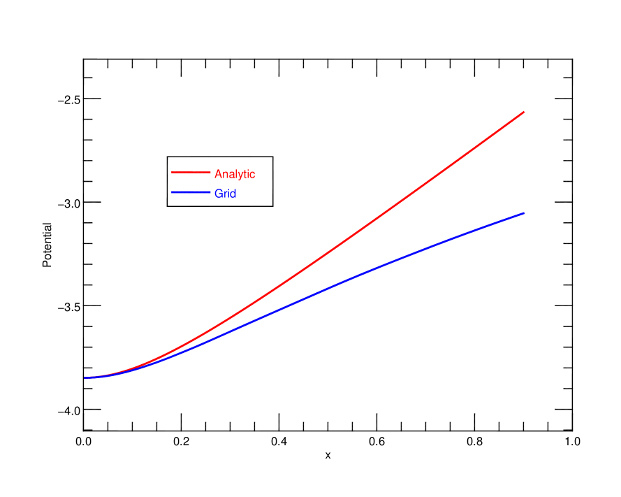
Figure 4.— Representative potential values along the major axis of a triaxial model. The red line indicates how the centrally-limited approximation would behave beyond its region of validity. The blue line represents the full NFW potential. We investigate orbits that move through regions where the difference between the potentials is significant.

With the full potential, we have generated surface of section plots to study a larger family of possible orbits. Figure  5 shows a surface of section plot for orbits with initial $y$ values $\approx 10^{-8}$ but varying initial $x$ and $z$ locations. Stable orbits form regular curves whereas unstable orbits appear as swarms of scattered points throughout regions of a surface of section plot. Orbits in the inner regions most typically show evidence of the instability, but there are also unstable regions for orbits which pass through areas where the difference between the approximate and full potentials seen in Figure 4 becomes significant. As a result of this extension to previous work, we conclude that the Adams instability should be present in any triaxial system with a cuspy inner profile, independent of the details of the potential further from the center. As cuspy cores are common results in N-body simulations of collapsing systems, we now turn to finding evidence of the Adams instability among them.

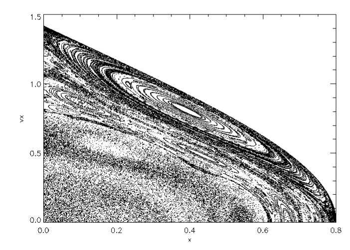
Figure 5.— Analogous to the surface of section plot in Figure 1b of Adams et al. (2007), this plot shows a slice through phase space that clearly delineates regions of regularity (smooth, connected curves) from irregularity. The axis ratios used match those in Adams et al. (2007) (3:4:5), but the full NFW potential is utilized. Each orbit has $|y|_{\rm initial}\leq 10^{-8}$ but varying $x$ and $z$ initial positions.

3. N-body Simulations

One of the main results of the Adams et al. (2007) work is the recognition that there is a specific signature of the instability. As an orbit experiences the instability, its position perpendicular to the principal plane in which it originally moved exponentially increases. We search for evidence of this behavior among the orbits that compose various N-body systems.

We have evolved systems with both $N=10^{5}$ and $N=10^{6}$ particles. All systems are initialized by randomly placing particles in spherical volume according to a prescribed density distribution. Typically, we will discuss models with Gaussian ($\rho\propto e^{-r^{2}}$) density distributions, but models with cuspy ($\rho\propto 1/r$) profiles have also been evolved. Past work has indicated little difference between the onset of the ROI in such systems when the amount of initial kinetic energy present is limited to induce triaxiality (Barnes, Lanzel, & Williams, 2009). For non-cosmological evolutions, this amounts to limiting the initial virial ratio of the system. We define the virial ratio as $Q=2T/|W|$, where $T$ and $W$ are the kinetic and gravitational potential energies, respectively. Velocity distributions are made initially isotropic by randomly orienting each particle’s velocity. Cosmological evolutions are started somewhat differently. The random component of the kinetic energy is limited and each particle’s initial velocity is a combination of Hubble expansion and isotropic random motion.

All N-body evolutions have been calculated using the publicly available GADGET-2 code (Springel, 2005). Simulations with $N=10^{5}$ use softening values $\delta=10^{-4}$. In $N=10^{6}$ simulations, evolution times are kept reasonable by adopting softening length values $\delta\propto N^{-1/2}$ (Power et al., 2003). Specifically, we set $\delta=4\times 10^{-3}$. Test runs with different values of $\delta$ have been performed and produce essentially identical results. Cosmological evolutions run between redshifts of nine and zero, while non-cosmological evolutions proceed for at least ten initial-system crossing times. The virial ratio behaves reasonably, with early oscillations settling down to the equilibrium value of one by the end of an evolution.

Periodic output files are analyzed in the post-evolution stage. Particle positions and velocities are used to determine axis ratio and energy behaviors as functions of time/redshift. The $x$, $y$, and $z$ axes are defined as the long, intermediate, and short axes of the system determined at the last output time. In cosmological simulations, all coordinates and velocities are comoving. All previous output values are transformed to this coordinate system for consistency. Examples of analysis products are presented in Figure 6. In general, our initially dynamically cold systems quickly deform to triaxial shapes followed by a longer-term relaxation towards sphericity.

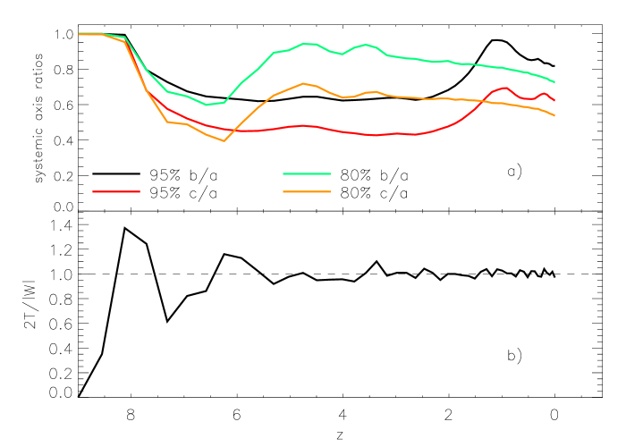
Figure 6.— Results from a cosmological evolution of a system with $N=10^{6}$, Gaussian initial density distribution, and zero initial random kinetic energy. Panel a shows the behavior of systemic axis ratios for two mass cutoff values. Using the innermost 80% of the mass in a system to determine axis ratios excludes many of the particles that are either escaping or near-escape as a result of such a cold collapse. Panel b illustrates the evolution of the virial ratio. This rapid approach to equilibrium is essentially the same for all of our evolutions.

We also filter for particles that are on orbits that should be susceptible to the Adams instability. Focusing on particles that are near the $x-z$ plane with small $y$-velocities gives us a subset that may show exponential growth perpendicular to the long axis of the system. Through trial-and-error, we have determined ranges of $y$-positions and velocities that balance the need to only look at particles with near-principal plane orbits with the desire to have as many particles as possible to analyze. Specifically, we demand that particles have $|y|\leq 10^{-4}$ and $|v_{y}|\leq 5\times 10^{-2}$ to be investigated further. We note that in varying these values, there are no changes to the qualitative behaviors we will now discuss. Simply tracking the numbers of particles that fit these constraints should provide a crude way to distinguish between the presence and absence of the instability. In the absence of the instability we expect the numbers of near-principal plane particles to be relatively steady. An example of this kind of behavior is shown in Figure 7. This figure corresponds to a non-cosmological simulation where there is enough initial kinetic energy to prevent triaxiality.

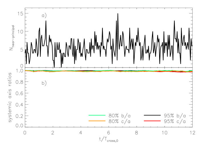
Figure 7.— Results from a non-cosmological evolution of a system with $N=10^{5}$, Gaussian initial density distribution, and just enough kinetic energy to avoid becoming triaxial (initial $Q=0.08$). Panel a shows the behavior of the number of particles in near-principal plane orbits. The near constancy of this value is seen in all of our non-cosmological evolutions, even those that result in triaxiality. Panel b illustrates the systemic axis ratios in the same way as in Figure 6. This model remains essentially spherical throughout its evolution.

Our hypothesis is that an active instability should depopulate near-principal plane orbits. As an active instability requires triaxiality, we present results from a simulation where the initial conditions are cold enough that the ROI will act. Figure 8 is analogous to Figure 7, but for a colder, non-cosmological system. Counter to our expectations, there is no obvious evolution of the number of near-principal-plane orbits. Another example of an evolution of near-principal-plane particles is shown in Figure 9. In this cosmological simulation, there is no initial random kinetic energy. The loss of near-principal plane orbits begins even as the system is still mostly spherical. When the system is most triaxial, the population seems rather stable. As the system moves towards a more spherical shape, the population rises again.

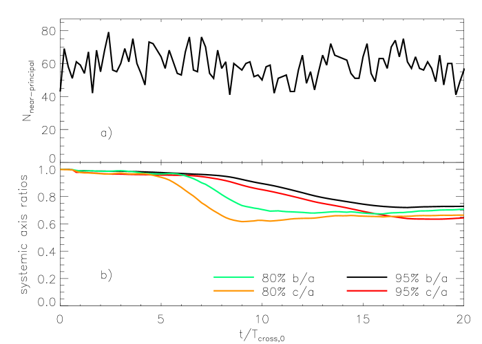
Figure 8.— Results from a non-cosmological evolution of a system with $N=10^{6}$, Gaussian initial density distribution, and not enough kinetic energy to avoid becoming triaxial (initial $Q=0.04$). The panels contain the same information as those in Figure 7. We note the same constant behavior of the number of near-principal-plane orbits even in the face of significant triaxiality in the system.

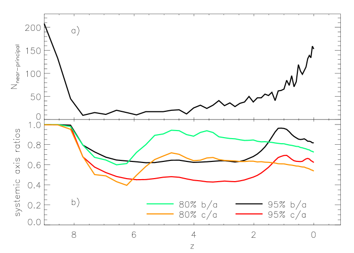
Figure 9.— Results from the same evolution shown in Figure 6. Panel a shows the behavior of the number of particles in near-principal plane orbits for a system. Unlike the analogous panel in Figure 7, there are two different trends in this behavior. There is a sharp initial decrease in the particles trapped near the principal plane. This decrease is seen only in systems with zero initial random kinetic energy (independent of cosmological expansion). Also, as redshift of zero is approached, this number climbs significantly. This late-time climb is common among all of the cosmological simulations we have run, independent of the duration and/or severity of the triaxiality induced. Panel b illustrates the corresponding systemic axis ratios. With the initial conditions we have investigated, all cosmological evolutions result in triaxiality. However, increasing the amount of initial random kinetic energy delays the onset of triaxiality.

In other cosmological simulations with non-zero initial random kinetic energy, plots analogous to Figure 9 lack the large initial value and subsequent decrease. The absence of any initial random velocities produces a sizeable population of orbits that satisfy our criteria for being near-principal plane, but subsequent evolution leads to random motion that remove them from consideration. Similar large decreases are also present in non-cosmological evolutions with zero initial kinetic energy. Apparently, the decrease seen in Figure 9 has nothing to do with the Adams instability. In the dynamically warmer cosmological simulations, triaxiality takes longer to develop, but the increase in near-principal-plane particles as $z=0$ is approached remains. Similar late-evolution increases are not present in any of our non-cosmological simulations. The cause of this difference is not clear at present.

We have also searched for a signal of the Adams instability in the behavior of individual orbits of masses in the N-body simulations. After identifying particles in near-principal plane orbits at a specified point in an evolution, we have tracked the subsequent positions of those particles for the remainder of the simulation. Plots of near-principal plane orbit behaviors are shown in Figure 10. At least some of the orbits show the same qualitative behavior as unstable orbits in smooth potentials. Numerous particles experience rapid rises in their positions perpendicular to the principal plane followed by a steady-state behavior. Unfortunately, a similar plot can be created starting at a point in time when the system is essentially spherical. The large changes in $y$-positions appear to happen even though the potential should not support the Adams instability. Without an unambiguous signal like the one shown in Figure 3b, and given that instability-like behavior occurs in spherical systems, the analysis of these N-body systems does not provide conclusive evidence of the Adams instability.

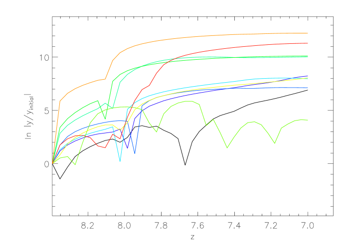
Figure 10.— Behavior of the $y$-positions of several particles in the same N-body simulation as in Figure 9. The starting point has been chosen so that it roughly agrees with the time when the system is beginning to become triaxial. Some orbits share the same qualitative behavior as Adams unstable orbits.

4. Investigating Discreteness Effects

The qualitative hints of the instability discussed above do provide some motivation to look beyond our simplest approaches. Given that there can be numerical effect competing with physical processes, we next turn to untangling any instability effects from finite-N effects by taking parallel tracks. We investigate how small-scale noise superimposed on a smooth background potential impacts the Adams instability. Separately, we analyze orbits in smoothed potentials derived from N-body simulations. The results of these investigations are described below.

Before moving on, we note that this discussion is not intended to imply that these simulations suffer from global-scale two-body effects. In previous work with similar models, we have found that neither mass segregation nor pervasive impulsive events occur (Barnes, Lanzel, & Williams, 2009). By these yardsticks, our simulations are collisionless.

We have added Gaussian perturbations to the smooth potentials described in Section 2. Specifically, each perturbation has the form,

$$\Phi_{\mathrm{pert}}(\mathbf{r})=A\exp{\left[\frac{-(\mathbf{r}-\mathbf{r}_{0})^{2}}{2\sigma_{p}^{2}}\right]},$$ (5)

with $A$ controlling the strength of the potential and $\mathbf{r}_{0}$ specifying its location. The width of the Gaussian $\sigma_{p}$ has been set to half the average distance between perturbers. Typically, thousands of perturbers are placed randomly throughout a potential. Using the orbit integration scheme described in Section 2, we have investigated the same range of initial conditions for these bumpy potentials.

For the values of $A$ and $\sigma_{p}$ adopted, we find that orbits that are stable in a smooth potential remain stable in a bumpy version. Conversely, smooth-potential unstable orbits remain unstable. We have been unable to convert stable orbits to unstable and vice versa. The two specific orbits resulting in Figures 11 and 12 illustrate this result. A broader range of orbit families have also been studied. Figure 13 shows various surfaces of section plots based on these families. The smooth potential underlying these plots is the same as the one used to create Figure 5. The panels highlight the lack of substantial changes as the perturbing strength changes. We interpret these results to mean that discreteness effects are not changing the basic structure of phase space. However, the time it takes an unstable orbit to reach its steady-state $y$-position decreases as the strength of the perturbations grows, as illustrated in Figure 11. The behaviors of the $y$-positions of orbits in our N-body simulations (e.g., Figure 10) are similar to those that result from encounters with strong perturbers. Specifically, the extremely rapid rise followed by a slower exponential increase leading to an eventual steady-state value is a common pattern. This supports the view that at least some of the motions away from the principal plane that occur in N-body simulations are caused by discreteness and not the Adams instability.

Figure 11.— Behaviors of an unstable orbit in a triaxial potential with $a=5$, $b=4$, $c=3$ and $|y|_{\rm initial}<10^{-8}$. Panels a through d correspond to perturbation strengths $10^{-5}$, $10^{-4}$, $10^{-3}$, and $10^{-2}$, respectively. The tell-tale exponential growth in the unstable $y$ direction is independent of the perturbing strength. However, as the perturbation strengthens, the time it takes for the particle to reach an equilibrium position decreases. Also, for the largest amplitudes studied, we note an almost immediate offset from zero develops before the exponential behavior begins.

Figure 12.— Behavior for an stable orbit in an gravitational potential with triaxial values $a=5$, $b=4$, $c=3$. The panels correspond to the same increase in perturbation strength shown in Figure 11. The signature of the Adams instability fails to appear at any perturbing strength investigated.

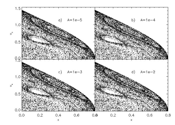
Figure 13.— Panels a through d again correspond to the same increasing perturbation strengths as in Figure 11. Each panel shows a surface of section plot based on orbits in triaxial potentials with $a=5$, $b=4$, $c=3$. Orbits take on a range of initial $x$ and $z$ positions, but $|y|_{\rm initial}<10^{-8}$. We interpret the lack of differences in the plots as evidence against the perturbers changing the overall character of orbits.

In order to test the possibility that the overall potentials do not have the appropriate shapes and/or profiles to support the Adams instability, we have also investigated the behavior of orbits in smoothed versions of our N-body simulations. Based on particle positions corresponding to highly triaxial states, we use a Gaussian kernel to smooth the mass distribution. Each particle is replaced by a Gaussian mass distribution with a prescribed scale length $\sigma_{s}$. This modifies that particle’s contribution to the potential at a point with displacement $\mathbf{r}$ by a term proportional to the error function of $r/\sigma_{s}$. Small $\sigma_{s}$ values (compared to the semiaxis lengths) result in essentially point-like behavior. For a given smoothed mass distribution, a grid of potential and force values are calculated. Again using the procedures in Section 2, a variety of initial conditions have been numerically integrated. As examples of the impact of smoothing on the orbits, Figure 14 shows segments of orbit paths derived from identical initial conditions in potentials with different smoothing lengths. The N-body model that serves as the basis for these potentials is spherical. The orbit is one that should run essentially through the center of the potential along the $x$-axis, if it were perfectly smooth. The discrete nature of the relatively unsmoothed ($\sigma_{s}=10^{-5}$) potential is evident.

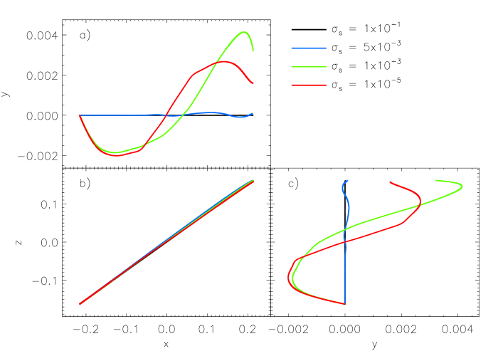
Figure 14.— Projections of orbits ($x-y$, $x-z$, and $y-z$ in panels a, b, and c, respectively) in four different potentials derived from a spherical N-body system. Each orbit starts with the same initial conditions. The smoothing lengths used to create the various potentials are given in the legend. For comparison, the initial system has a radius of one. As expected, the impact of discreteness decreases with increasing smoothing length.

Figure 15 shows the signature of the Adams instability for a particle orbiting in a highly smoothed ($\sigma_{s}=0.1$) version of a triaxial $c/a\approx 0.5,b/a\approx 0.7$ N-body potential. In line with the previous findings of this section, we see the same signature in potentials with smaller smoothing lengths, but the “rise time” of the instability decreases with the smoothing length.

Figure 15.— The $y$-positions of orbits in smoothed versions of a triaxial N-body potential. Panels a, b, c, and d correspond to smoothing lengths $\sigma_{s}=1\times 10^{-1}$, $\sigma_{s}=5\times 10^{-3}$, $\sigma_{s}=1\times 10^{-3}$, and $\sigma_{s}=1\times 10^{-5}$, respectively. The orbits all have the same initial conditions. The positions are normalized to the initial value, which is $\approx 10^{-8}$. The exponential growth inherent with the Adams instability is evident, and the orbits show the same qualitative behavior as those in Section 2. The major distinction between the panels is that the steady-state $y$-position is reached more rapidly in less smoothed potentials.

Overall, these findings suggest that numerical issues can conflate physical processes to disguise the presence of the Adams instability. The specific signature of the instability seen in smooth potentials has its quantitative details altered by finite-N effects, but the qualitative behavior remains.

5. Conclusions

Numerous previous studies have investigated how initially spherical N-body systems become triaxially distorted during self-gravitating evolution. The most common explanation involves what has become known as the radial orbit instability. Axes along which more mass resides in these simulations can strongly influence the tangential motions of neighboring orbits, causing alignments which lead to non-sphericity. However, these systems do not evolve to extreme triaxiality, as one would expect if the radial orbit instability operated continuously. We have investigated a way in which the growth of triaxiality in simulations of collapsing systems could be halted. Beginning with a previously examined orbital instability that occurs in triaxial systems (Adams et al., 2007), we have shown that what we term the Adams instability persists beyond the centrally-limited situation originally investigated. The Adams instability gives rise to a characteristic exponential growth in position perpendicular to a principal axis. In this way, triaxial-supporting orbits can be depopulated.

To determine the presence of the Adams instability in simulations, we have created and analyzed evolutions of N-body systems from a variety of initial conditions. Following previous work, we control the amount of initial random kinetic energy present in the systems to create both spherical and triaxial evolutions. Particle number, softening length, and the presence of cosmological expansion have all been varied for our investigation. By tracking orbits near principal planes of systems, we have seen the signature of the Adams instability. However, this signature also appears in systems that are essentially spherical. Individual orbits of particles making up N-body systems do not provide unambiguous evidence for the Adams instability.

After creating perturbed versions of the smooth potentials used to discover the Adams instability, we have found that small-scale noise, like that due to discreteness effects in an N-body simulation, can make the onset of the instability more rapid. However, the perturbations studied cannot change an orbit that would be stable in a smooth potential into an unstable one, and vice versa. The behavior of orbits in sufficiently perturbed potentials does mirror what is seen in our N-body evolutions.

We have also looked for the Adams instability in smoothed versions of our N-body systems. Fixed-time snapshots of our systems have been used to create smoothed potentials. Tracking orbital motions of particular initial conditions as the smoothing length changes shows that these potentials will support the Adams instability. It appears that a combination of discreteness effects and the Adams instability are present in N-body simulations like ours. Numerical effects can disguise the quantitative outcomes of the instability, but they cannot erase its qualitative behavior. Given that physical systems should be essentially free of discreteness effects, the inability to quantify the contributions of the two mechanisms to simulated end-state shapes gives makes questionable any simulation-based prediction of impact on the shapes of real-world systems.

References

- Adams et al. (2007) Adams, F.C., Bloch, A.M., Butler, S.C., Druce, J. M., Ketchum, J.A. 2007, ApJ, 670, 1027
- Allgood et al. (2006) Allgood, B., Flores, R.A., Primack, J.R., Kravtsov, A.V., Wechsler, R.H., Faltenbacher, A., Bullock, J.S. 2006, MNRAS, 367, 1781
- Bailin & Steinmetz (2005) Bailin, J., Steinmetz, M. 2005, ApJ, 627, 647
- Bardeen et al. (1986) Bardeen, J.M., Bond, J.R., Kaiser, N., Szalay, A.S. 1986, ApJ, 304, 15
- Barnes & Efstathiou (1987) Barnes, J., Efstathiou, G. 1987, ApJ, 319, 575
- Barnes et al. (2005) Barnes, E.I., Williams, L.L.R., Babul, A., Dalcanton, J.J. 2005, ApJ, 634, 775
- Barnes, Lanzel, & Williams (2009) Barnes, E.I., Lanzel, P.A., Williams, L.L.R. 2009, ApJ, 704, 372
- Bellovary et al. (2008) Bellovary, J.M., Dalcanton, J.J., Babul, A., Quinn, T.R., Maas, R.W., Austin, C.G., Williams, L.L.R., Barnes, E.I. 2008, ApJ, 685, 739
- Benhaiem & Sylos Labini (2015) Benhaiem, D., Sylos Labini, F. 2015, MNRAS, 448, 2634
- Binney (1981) Binney, J. 1981, MNRAS, 196, 455
- Binney & Tremaine (1987) Binney, J., Tremaine, S. 1987, Galactic Dynamics (Princeton, NJ: Princeton Univ. Press)
- Chandrasekhar (1969) Chandrasekhar, S. 1969, Ellipsoidal Figures of Equilibrium (New Haven, CT: Yale Univ. Press)
- Dubinski & Carlberg (1991) Dubinski, J., Carlberg, R.G. 1991, ApJ, 378, 496
- Frenk et al. (1988) Frenk, C.S., White, S.D.M., Davis, M., Efstathiou, G. 1988, ApJ, 327, 507
- Hernquist (1990) Hernquist, L. 1990, ApJ, 356, 359
- Jing & Suto (2002) Jing, Y.P., Suto, Y. 2002, ApJ, 574, 538
- Merritt & Aguilar (1985) Merritt, D., Aguilar, L.A. 1985, MNRAS, 217, 787
- Merritt & Fridman (1996) Merritt, D., Fridman, T. 1996, ApJ, 460, 136
- Navarro, Frenk, & White (1996) Navarro, J.F., Frenk, C.S., White, S.D.M. 1996, ApJ, 462, 563
- Palmer & Papaloizou (1987) Palmer, P.L., Papaloizou, J. 1987, MNRAS, 224, 1043
- Poon & Merritt (2001) Poon, M.Y., Merritt, D. 2001, ApJ, 549, 192
- Power et al. (2003) Power, C., Navarro, J.F., Jenkins, A., Frenk, C.S., White, S.D.M., Springel, V., Stadel, J., Quinn, T. 2003, MNRAS, 338, 14
- Press et al. (1994) Press, W.H., Teukolsky, S.A., Vetterling, W.T., Flannery, B.P. 1994, Numerical Recipes (Cambridge, UK: Cambridge Univ. Press)
- Shaya et al. (2010) Shaya, E., Olling, R., Ricotti, M., Majewski, S.R., Patterson, R.J., Allen, R., van der Marel, R., Brown, W., Bullock, J., Burkert, A., Combes, F., Gnedin, O., Grillmair, C., Kulkarni, S., Guhathakurta, P., Helmi, A., Johnston, K., Kroupa, P., Lake, G., Moore, B., Tully, R.B. 2010, Astro2010: The Astronomy and Astrophysics Decadal Survey, Science White Papers, no. 274
- Springel (2005) Springel, V. 2005, MNRAS, 364, 1105