A balance index for phylogenetic trees based on rooted quartets

Abstract

We define a new balance index for rooted phylogenetic trees based on the symmetry of the evolutive history of every set of 4 leaves. This index makes sense for multifurcating trees and it can be computed in time linear in the number of leaves. We determine its maximum and minimum values for arbitrary and bifurcating trees, and we provide exact formulas for its expected value and variance on bifurcating trees under Ford’s $\alpha$-model and Aldous’ $\beta$-model and on arbitrary trees under the $\alpha$-$\gamma$-model.

1 Introduction

One of the most broadly studied properties of the topology of rooted phylogenetic trees is their balance, that is, the tendency of the subtrees rooted at all children of any given node to have a similar shape. The main reason for this interest is that the balance of a rooted tree embodies the symmetry of the evolutive history it describes, and hence it reflects, at least to some extent, a feature of the forces that drove the evolution of the set of species represented in the tree; see Chapter 33 of [12].

The balance of a tree is usually quantified by means of balance indices. The two most popular such indices are Colless’ index [8] for bifurcating trees, which is defined as the sum, over all internal nodes $v$, of the absolute value of the difference between the number of descendant leaves of the pair of children of $v$, and Sackin’s index [25, 26], which is defined, for arbitrary trees, as the sum of the depths of all leaves in the tree. But many other balance indices have been proposed in the literature, like for instance, for bifurcating trees, the variance of the depths of the leaves [16, 25], the sum of the reciprocals of the orders of the rooted subtrees [26], and the number of cherries [19], and, for arbitrary trees, the total cophenetic index [20] and a generalization of the Colless index [21]. For more indices, see again Chapter 33 in the book by Felsenstein [12]. All these balance indices depend only on the topology of the trees, not on the branch lengths or the actual labels on their leaves, although the balance of time-stamped trees has also been considered by Dearlove and Frost [11]. This abundance of balance indices is partly motivated by the advice given by Shao and Sokal [26] to use more than one such index to quantify the balance of a tree, as well as by their use as tools to test stochastic models of evolution [4, 15, 16, 22, 26]; other properties of the shapes of phylogenetic trees used in this connection include the distribution of clades’ sizes [30, 31] and the joint distribution of the numbers of rooted subtrees of different types [28].

In this paper we propose a new balance index, the rooted quartet index. To define it, we associate to each 4-tuple of different leaves of the tree $T$ a value that quantifies the symmetry of the joint evolution of the species they represent, in the sense that it grows with the number of isomorphisms of the restriction of $T$ to them (the rooted quartet they define), and then we add up these values over all 4-tuples of different leaves of $T$. The idea behind the definition of this balance index is that a highly symmetrical evolutive process should give rise to symmetrical evolutive histories of many small subsets of taxa. In terms of phylogenetic trees, this leads us to expect that, the most symmetrical a phylogenetic tree is, the most symmetrical will be its restrictions to subsets of leaves of a fixed cardinality. Since the smallest number of leaves yielding enough different tree topologies to allow a meaningful comparison of their symmetry is 4, we assess the balance of a tree by measuring the symmetry of all its rooted quartets and adding up the results. And indeed, in Section 4 below we shall find the trees with maximum and minimum values of our rooted quartet index in both the arbitrary and the bifurcating cases, and it will turn out that the minimum value is reached exactly at the combs (see Fig. 1.(a)), which are usually considered the least balanced trees, and the maximum value is reached, in the arbitrary case, exactly at the rooted stars (see Fig. 1.(b)) and, in the bifurcating case, exactly at the maximally balanced trees (cf. Fig. 3 ), which in both cases are considered the most balanced trees.

Besides taking its maximum and minimum values at the expected trees, other important features of our index are that it can be easily computed in linear time and that its mean value and variance can be explicitly computed on any probabilistic model of phylogenetic trees satisfying two natural conditions: independence under relabelings and sampling consistency. This allows us to provide these values for two well-known probabilistic models of bifurcating phylogenetic trees, Ford’s $\alpha$-model [13] and Aldous’ $\beta$-model [2], which include as specific instances the Yule [14, 29] and the uniform [6, 24, 19] models, as well as for Chen-Ford-Winkel’s $\alpha$-$\gamma$-model of multifurcating trees [7]. To our knowledge, this is the first shape index for which closed formulas for the expected value and the variance under the $\alpha$-$\gamma$-model have been provided.

The rest of this paper is organized as follows. In the next section we introduce the basic notations and facts on phylogenetic trees that will be used in the rest of the paper, and we recall several preliminary results on probabilistic models of phylogenetic trees, proving those results for which we have not been able to find a suitable reference in the literature. Then, in Section 3, we define our rooted quartet index $\mathit{rQI}$ and we establish its basic properties. In Section 4 we compute its maximum and minimum values, and finally, in Section 5, we compute its expected value and variance under different probabilistic models. This paper is accompanied by the GitHub page https://github.com/biocom-uib/Quartet_Index containing a set of Python scripts that perform several computations related to this index.

2 Preliminaries

2.1 Notations and conventions

In this paper, by an (unlabeled) tree we mean a rooted tree without out-degree 1 nodes. As it is usual, we understand such a tree as a directed graph, with its arcs pointing away from the root. A tree is bifurcating when all its internal nodes have out-degree 2; when we want to emphasize that a tree need not be bifurcating, we shall call it multifurcating. We shall denote by $L(T)$ the set of leaves of a tree $T$, by $V_{int}(T)$ its set of internal nodes, and by $\mathrm{child}(u)$ the set of children of an internal node $u$, that is, those nodes $v$ such that $(u,v)$ is an arc in $T$. We shall always consider two isomorphic trees as equal, and we shall denote by $\mathcal{T}^{*}_{n}$ and $\mathcal{BT\!}^{*}_{n}$ the sets of (isomorphism classes of) multifurcating trees and of bifurcating trees with $n$ leaves, respectively.

A phylogenetic tree on a set $\Sigma$ is a tree with its leaves bijectively labeled in $\Sigma$. An isomorphism of phylogenetic trees is an isomorphism of trees that preserves the leaves’ labels. To simplify the language, we shall always identify a leaf of a phylogenetic tree with its label and we shall say that two isomorphic phylogenetic trees “are the same”. We shall denote by $\mathcal{T}(\Sigma)$ and $\mathcal{BT\!}(\Sigma)$ the sets of (isomorphism classes of) multifurcating phylogenetic trees and of bifurcating phylogenetic trees on $\Sigma$, respectively. If $\Sigma$ and $\Sigma^{\prime}$ are any two sets of labels of the same cardinality, say $n$, then any bijection $\Sigma\leftrightarrow\Sigma^{\prime}$ extends in a natural way to bijections $\mathcal{T}(\Sigma)\leftrightarrow\mathcal{T}(\Sigma^{\prime})$ and $\mathcal{BT\!}(\Sigma)\leftrightarrow\mathcal{BT\!}(\Sigma^{\prime})$. When the specific set of labels $\Sigma$ is irrelevant and only its cardinality matters, we shall write $\mathcal{T}_{n}$ and $\mathcal{BT\!}_{n}$ (with $n=|\Sigma|$) instead of $\mathcal{T}(\Sigma)$ and $\mathcal{BT\!}(\Sigma)$, and we shall identify $\Sigma$ with the set $[n]=\{1,2,\ldots,n\}$. If $|\Sigma|=n$, there exists a forgetful mapping $\pi:\mathcal{T}(\Sigma)\to\mathcal{T}_{n}^{*}$ that sends every phylogenetic tree $T$ on $\Sigma$ to its underlying unlabeled tree: we shall call $\pi(T)$ the shape of $T$. We shall write $T_{1}\equiv T_{2}$ to denote that two phylogenetic trees $T_{1},T_{2}$ (possibly on different sets of labels of the same cardinality) have the same shape.

We shall represent trees and phylogenetic trees by means of their usual Newick format, although we shall omit the ending mark “;” in order not to confuse it in the text with a semicolon punctuation mark. In the case of (unlabeled) trees, we shall denote the leaves with $*$ symbols.

Given two nodes $u,v$ in a tree $T$, we say that $v$ is a descendant of $u$, and also that $u$ is an ancestor of $v$, when there exists a path from $u$ to $v$ in $T$; this, of course, includes the case of the stationary path from a node $u$ to itself, and hence, in this context, we shall use the adjective proper to mean that $u\neq v$. Given a node $v$ of a tree $T$, the subtree $T_{v}$ of $T$ rooted at $v$ is the subgraph of $T$ induced by the descendants of $v$. We shall denote by $\kappa_{T}(v)$, or simply by $\kappa(v)$ if $T$ is implicitly understood, the number of leaves of $T_{v}$.

Given a tree $T$ and a subset $X\subseteq L(T)$, the restriction $T(X)$ of $T$ to $X$ is the tree obtained by first taking the subgraph of $T$ induced by all the ancestors of leaves in $X$ and then suppressing its out-degree 1 nodes. By suppressing a node $u$ with out-degree 1 we mean that if $u$ is the root, we remove it together with the arc incident to it, and, if $u$ is not the root and if $u^{\prime}$ and $u^{\prime\prime}$ are, respectively, its parent and its child, then we remove the node $u$ and the arcs $(u^{\prime},u),(u,u^{\prime\prime})$ and we replace them by a new arc $(u^{\prime},u^{\prime\prime})$. For every $Y\subseteq L(T)$, the tree $T(-Y)$ obtained by removing $Y$ from $T$ is nothing but the restriction $T(L(T)\setminus Y)$. If $T$ is a phylogenetic tree on a set $\Sigma$ and $X\subseteq\Sigma$, the restrictions $T(X)$ and $T(-X)$ are phylogenetic trees on $X$ and $\Sigma\setminus X$, respectively.

A comb is a bifurcating phylogenetic tree such that all its internal nodes have a leaf child: see Fig. 1.(a). All combs with the same number $n$ of leaves have the same shape, and we shall generically denote them (as well as their shape in $\mathcal{T}_{n}^{*}$) by $K_{n}$. A rooted star is a phylogenetic tree all of whose leaves are children of the root: see Fig. 1.(b). For every set $\Sigma$, there is only one rooted star on $\Sigma$, and if $|\Sigma|=n$, we shall generically denote it (as well as its shape) by $S_{n}$.

Figure 1: (a) A comb $K_{n}$. (b) A rooted star $S_{n}$.

Given $k\geqslant 2$ phylogenetic trees $T_{1},\ldots,T_{k}$, with every $T_{i}\in\mathcal{T}(\Sigma_{i})$ and the sets of labels $\Sigma_{i}$ pairwise disjoint, their root join is the phylogenetic tree $T_{1}\star T_{2}\star\cdots\star T_{k}$ on $\bigcup_{i=1}^{k}\Sigma_{i}$ obtained by connecting the roots of (disjoint copies of) $T_{1},\ldots,T_{k}$ to a new common root $r$; see Fig. 2. If $T_{1},\ldots,T_{k}$ are unlabeled trees, a similar construction yields a tree $T_{1}\star\cdots\star T_{k}$.

Figure 2: The root join $T_{1}\star\cdots\star T_{k}$.

Let $T$ be a bifurcating tree. For every $v\in V_{int}(T)$, say with children $v_{1},v_{2}$, the balance value of $v$ is $bal_{T}(v)=|\kappa(v_{1})-\kappa(v_{2})|$. An internal node $v$ of $T$ is balanced when $bal_{T}(v)\leqslant 1$. So, a node $v$ with children $v_{1}$ and $v_{2}$ is balanced if, and only if, $\{\kappa(v_{1}),\kappa(v_{2})\}=\{\lfloor\kappa(v)/2\rfloor,\lceil\kappa(v)/2\rceil\}$. We shall say that a bifurcating tree $T$ is maximally balanced when all its internal nodes are balanced. Recursively, a bifurcating tree is maximally balanced when its root is balanced and the subtrees rooted at the children of the root are both maximally balanced. This implies that, for any fixed number $n$ of nodes, there is only one maximally balanced tree in $\mathcal{BT\!}_{n}^{*}$; see Section 2.1 in [20]. Fig. 3 depicts the maximally balanced trees with $n=6,7,8$ leaves. When $n$ is a power of 2, the maximally balanced bifurcating tree with $n$ leaves is the fully symmetric bifurcating tree, where, for each internal node, the pair of subtrees rooted at its children are isomorphic; see again Fig. 3 for $n=8$.

Figure 3: The shapes of the maximally balanced trees with 6, 7, and 8 leaves. The tree with 8 leaves is fully symmetric.

2.2 Probabilistic models

A probabilistic model of phylogenetic trees $P_{n}$, $n\geqslant 1$, is a family of probability mappings $P_{n}:\mathcal{T}_{n}\to[0,1]$, each one sending each phylogenetic tree in $\mathcal{T}_{n}$ to its probability under this model. Every such a probabilistic model of phylogenetic trees $P_{n}$ induces a probabilistic model of trees, that is, a family of probability mappings $P^{*}_{n}:\mathcal{T}^{*}_{n}\to[0,1]$, by defining the probability of a tree as the sum of the probabilities of all phylogenetic trees in $\mathcal{T}_{n}$ with that shape:

$$P^{*}_{n}(T^{*})=\sum_{T\in\mathcal{T}_{n}\atop\pi(T)=T^{*}}P_{n}(T).$$

If $|\Sigma|=n$, then $P_{n}:\mathcal{T}_{n}\to[0,1]$ induces also a probability mapping $P_{\Sigma}$ on $\mathcal{T}(\Sigma)$ through the bijection $\mathcal{T}_{\Sigma}\leftrightarrow\mathcal{T}_{n}$ induced by a given bijection $\Sigma\leftrightarrow[n]$.

A probabilistic model of bifurcating phylogenetic trees is a probabilistic model of phylogenetic trees $P_{n}$ such that $P_{n}(T)=0$ for every $T\in\mathcal{T}_{n}\setminus\mathcal{BT\!}_{n}$.

A probabilistic model of phylogenetic trees $P_{n}$ is shape invariant (or exchangeable, according to Aldous [2]) when, for every $T,T^{\prime}\in\mathcal{T}_{n}$, if $T\equiv T^{\prime}$, then $P_{n}(T)=P_{n}(T^{\prime})$. In this case, for every $T^{*}\in\mathcal{T}_{n}^{*}$ and for every $T\in\pi^{-1}(T^{*})$,

$$P_{n}^{*}(T^{*})=\big{|}\{T^{\prime}\in\mathcal{T}_{n}:\pi(T^{\prime})=T^{*}\}\big{|}\cdot P_{n}(T).$$

Conversely, every probabilistic model of trees $P^{*}_{n}$ defines a shape invariant probabilistic model of phylogenetic trees $P_{n}$ by means of

$$P_{n}(T)=\frac{P_{n}^{*}(\pi(T))}{\big{|}\{T^{\prime}\in\mathcal{T}_{n}:T^{\prime}\equiv T\}\big{|}}.$$ (1)

Notice that if $P_{n}$ is shape invariant, then, for every set of labels $\Sigma$, say, with $|\Sigma|=n$, the probability mapping $P_{\Sigma}:\mathcal{T}(\Sigma)\to[0,1]$ induced by the mapping $P_{n}$ does not depend on the specific bijection $\Sigma\leftrightarrow[n]$ used to define it.

A probabilistic model of phylogenetic trees $P_{n}$ is sampling consistent [2] (or also deletion stable, according to Ford [13]) when, for every $n\geqslant 2$, if we choose a tree $T\in\mathcal{T}_{n}$ with probability distribution $P_{n}$ and we remove its leaf $n$, the resulting tree is obtained with probability distribution $P_{n-1}$; formally, when, for every $n\geqslant 2$ and for every $T_{0}\in\mathcal{T}_{n-1}$,

$$P_{n-1}(T_{0})=\sum_{T\in\mathcal{T}_{n}\atop T(-n)=T_{0}}P_{n}(T).$$

It is straightforward to prove, by induction on $n-m$ and using that, for every $T\in\mathcal{T}_{n}$ and for every $1\leqslant m<n$, the restriction of $T(-n)$ to $[m]$ is simply $T([m])$, that this condition is equivalent to the following: $P_{n}$ is sampling consistent when, for every $n\geqslant 2$, for every $1\leqslant m<n$, and for every $T_{0}\in\mathcal{T}_{m}$,

$$P_{m}(T_{0})=\sum_{T\in\mathcal{T}_{n}\atop T([m])=T_{0}}P_{n}(T).$$ (2)

It is also easy to prove that if $P_{n}$ is sampling consistent and shape invariant, so that the probability of a phylogenetic tree is not affected by permutations of its leaves, then, for every $n\geqslant 2$, for every $\emptyset\neq X\subsetneq[n]$, say, with $|X|=m$, and for every $T_{0}\in\mathcal{T}(X)$,

$$P_{X}(T_{0})=\sum_{T\in\mathcal{T}_{n}\atop T(X)=T_{0}}P_{n}(T).$$

(where $P_{X}$ stands for the probability mapping on $\mathcal{T}(X)$ induced by $P_{m}$ through any bijection $X\leftrightarrow\big{[}m\big{]}$).

A probabilistic model of trees $P^{*}_{n}$ is sampling consistent when, for every $n\geqslant 2$, if we choose a tree $T\in\mathcal{T}_{n}^{*}$ with probability distribution $P^{*}_{n}$ and a leaf $x\in L(T)$ equiprobably and if we remove $x$ from $T$, the resulting tree is obtained with probability distribution $P_{n-1}^{*}$: formally, when, for every $n\geqslant 2$ and for every $T_{0}\in\mathcal{T}^{*}_{n-1}$,

$$P^{*}_{n-1}(T_{0})=\sum_{T\in\mathcal{T}_{n}^{*}}\frac{\big{|}\{x\in L(T):T(-x)=T_{0}\}\big{|}}{n}\cdot P^{*}_{n}(T).$$

We prove now several lemmas on probabilistic models that will be used in Section 5. The first lemma provides an extension of equation (2) to trees; we include it because we have not been able to find a suitable reference for it in the literature. In it, and henceforth, $\mathcal{P}_{k}(X)$ denotes the set of all subsets of cardinality $k$ of $X$.

Lemma 1.

A probabilistic model of trees $P^{*}_{n}$ is sampling consistent if, and only if, for every $n\geqslant 2$, for every $1\leqslant m<n$, and for every $T_{0}\in\mathcal{T}^{*}_{m}$,

$$P^{*}_{m}(T_{0})=\sum_{T\in\mathcal{T}_{n}^{*}}\frac{\big{|}\{X\in\mathcal{P}_{m}(L(T)):T(X)=T_{0}\}\big{|}}{\binom{n}{m}}\cdot P^{*}_{n}(T).$$

Proof.

The “if” implication is obvious. As far as the “only if” implication goes, we prove by induction on $n-m$ that if $P^{*}_{n}$ is sampling consistent, then, for every $T_{0}\in\mathcal{T}^{*}_{m}$,

$$P^{*}_{m}(T_{0})=\sum_{T_{n}\in\mathcal{T}_{n}^{*}}\frac{\big{|}\{X\in\mathcal{P}_{n-m}(L(T_{n})):T_{n}(-X)=T_{0}\}\big{|}}{\binom{n}{m}}\cdot P^{*}_{n}(T_{n}).$$

The starting case $m=n-1$ is the sampling consistency property. Assume now that this equality holds for $m$ and let $T_{0}\in\mathcal{T}^{*}_{m-1}$. Then

$$\begin{array}[]{l}P_{m-1}^{*}(T_{0})\displaystyle=\sum_{T_{m}\in\mathcal{T}_{m}^{*}}\frac{\big{|}\{x\in L(T_{m}):T_{m}(-x)=T_{0}\}\big{|}}{m}\cdot P^{*}_{m}(T_{m})\\ \qquad\mbox{(by the sampling consistency)}\\[4.30554pt] \displaystyle=\sum_{T_{m}\in\mathcal{T}_{m}^{*}}\Bigg{(}\frac{\big{|}\{x\in L(T_{m}):T_{m}(-x)=T_{0}\}\big{|}}{m}\\[4.30554pt] \hskip 56.9055pt\displaystyle\cdot\sum_{T_{n}\in\mathcal{T}_{n}^{*}}\frac{\big{|}\{X\in\mathcal{P}_{n-m}(L(T_{n})):T_{n}(-X)=T_{m}\}\big{|}}{\binom{n}{m}}\cdot P_{n}^{*}(T_{n})\Bigg{)}\\[4.30554pt] \qquad\mbox{(by the induction hypothesis)}\\[4.30554pt] \displaystyle=\sum_{T_{m}\in\mathcal{T}_{m}^{*}}\sum_{T_{n}\in\mathcal{T}_{n}^{*}}\Bigg{(}\frac{\big{|}\{x\in L(T_{m}):T_{m}(-x)=T_{0}\}\big{|}}{m}\\[4.30554pt] \hskip 71.13188pt\displaystyle\cdot\frac{\big{|}\{X\in\mathcal{P}_{n-m}(L(T_{n})):T_{n}(-X)=T_{m}\}\big{|}}{\binom{n}{m}}\Bigg{)}\cdot P_{n}^{*}(T_{n})\\[4.30554pt] \displaystyle=\sum_{T_{n}\in\mathcal{T}_{n}^{*}}\frac{\big{|}\{(X,x)\in\mathcal{P}_{n-m}(L(T_{n}))\times(L(T_{n})\setminus X):(T_{n}(-X))(-x)=T_{0}\}\big{|}}{m\cdot\binom{n}{m}}\cdot P_{n}^{*}(T_{n})\\[8.61108pt] \displaystyle=\sum_{T_{n}\in\mathcal{T}_{n}^{*}}\frac{\big{|}\{(X,x)\in\mathcal{P}_{n-m}(L(T_{n}))\times(L(T_{n})\setminus X):(T_{n}(-(X\cup\{x\}))=T_{0}\}\big{|}}{m\cdot\binom{n}{m}}\cdot P_{n}^{*}(T_{n})\\[8.61108pt] \displaystyle=\sum_{T_{n}\in\mathcal{T}_{n}^{*}}\frac{(n-m+1)\big{|}\{Y\in\mathcal{P}_{n-m+1}(L(T_{n})):T_{n}(-Y)=T_{0}\}\big{|}}{m\cdot\binom{n}{m}}\cdot P_{n}^{*}(T_{n})\\[8.61108pt] \displaystyle=\sum_{T_{n}\in\mathcal{T}_{n}^{*}}\frac{\big{|}\{Y\in\mathcal{P}_{n-m+1}(L(T_{n})):T_{n}(-Y)=T_{0}\}\big{|}}{\binom{n}{m-1}}\cdot P_{n}^{*}(T_{n})\end{array}$$

which proves the inductive step. ∎∎

Lemma 2.

Let $P_{n}$ be a shape invariant probabilistic model of phylogenetic trees. For every $T_{n-1},T_{n-1}^{\prime}\in\mathcal{T}_{n-1}$, if $T_{n-1}\equiv T_{n-1}^{\prime}$, then

$$\sum_{T_{n}\in\mathcal{T}_{n}\atop T_{n}(-n)=T_{n-1}}P_{n}(T_{n})=\sum_{T^{\prime}_{n}\in\mathcal{T}_{n}\atop T^{\prime}_{n}(-n)=T^{\prime}_{n-1}}P_{n}(T^{\prime}_{n}).$$

Proof.

Let $T_{n-1}^{*}=\pi(T_{n-1})=\pi(T^{\prime}_{n-1})$ and let $f:T_{n-1}\to T^{\prime}_{n-1}$ be an isomorphism of unlabeled trees, which exists because $T_{n-1}$ and $T_{n-1}^{\prime}$ are both isomorphic as unlabeled trees to their shape $T_{n-1}^{*}$. For every $T\in\mathcal{T}_{n-1}$, let

$$E_{n}(T)=\{T_{n}\in\mathcal{T}_{n}:T_{n}(-n)=T\}.$$

Each $T_{n}$ in $E_{n}(T_{n-1})$ is obtained by adding a leaf $n$ to $T_{n-1}$ as a new child either to an internal node, or to a new node obtained by splitting an arc into two consecutive arcs, or to a new bifurcating root (whose other child would be the old root). This entails the existence of a shape preserving bijection

$$\Phi:E_{n}(T_{n-1})\rightarrow E_{n}(T^{\prime}_{n-1})$$

that sends each $T_{n}\in E_{n}(T_{n-1})$ to the phylogenetic tree $\Phi(T_{n})$ obtained by adding the leaf $n$ to $T_{n-1}^{\prime}$ at the place corresponding through the isomorphism $f$ to the place where it has been added to $T_{n-1}$. Then, since $P_{n}$ is shape invariant,

$$\sum_{T_{n}\in E(T_{n-1})}P_{n}(T_{n})=\sum_{T_{n}\in E(T_{n-1})}P_{n}(\Phi(T_{n}))=\sum_{T^{\prime}_{n}\in E(T^{\prime}_{n-1})}P_{n}(T^{\prime}_{n})$$

as we claimed. ∎∎

Next lemma generalizes Cor. 40 of [13]. For the sake of completeness, we provide a direct complete proof of it.

Lemma 3.

Let $P_{n}$ be a shape invariant probabilistic model of phylogenetic trees and let $P^{*}_{n}$ be the corresponding probabilistic model of trees. Then, $P_{n}$ is sampling consistent if, and only if, $P^{*}_{n}$ is sampling consistent.

Proof.

Let us prove first the “only if” implication. Let $P_{n}$ be sampling consistent. Then, for every $T_{n-1}^{*}\in\mathcal{T}_{n-1}^{*}$ and for every $\widehat{T}_{n-1}\in\pi^{-1}(T_{n-1}^{*})$,

$$\begin{array}[]{l}\displaystyle P_{n-1}^{*}(T_{n-1}^{*})=\big{|}\{T_{n-1}\in\mathcal{T}_{n-1}:\pi(T_{n-1})=T_{n-1}^{*}\}\big{|}\cdot P_{n-1}(\widehat{T}_{n-1})\\ \qquad\mbox{(by the shape invariance of $P_{n}$)}\\ \quad\displaystyle=\big{|}\{T_{n-1}\in\mathcal{T}_{n-1}:\pi(T_{n-1})=T_{n-1}^{*}\}\big{|}\cdot\sum_{T_{n}\in\mathcal{T}_{n}\atop T_{n}(-n)=\widehat{T}_{n-1}}P_{n}(T_{n})\\ \qquad\mbox{(by the sampling consistency of $P_{n}$)}\\ \quad\displaystyle=\sum_{T_{n-1}\in\pi^{-1}(T_{n-1}^{*})}\sum_{T_{n}\in\mathcal{T}_{n}\atop T_{n}(-n)={T}_{n-1}}P_{n}(T_{n})\\ \qquad\mbox{(by Lemma \ref{lem:prevT})}\\ \quad\displaystyle=\sum_{T_{n}\in\mathcal{T}_{n}\atop\pi(T_{n}(-n))=T_{n-1}^{*}}P_{n}(T_{n})=\sum_{T_{n}\in\mathcal{T}_{n}\atop\pi(T_{n}(-i))=T_{n-1}^{*}}P_{n}(T_{n})\quad\mbox{for every $i=1,\ldots,n$}\\ \qquad\mbox{(by the shape invariance of $P_{n}$).}\\ \end{array}$$

Therefore

$$\begin{array}[]{l}\displaystyle n\cdot P_{n-1}^{*}(T_{n-1}^{*})=\sum_{i=1}^{n}\sum_{T_{n}\in\mathcal{T}_{n}\atop\pi(T_{n}(-i))=T_{n-1}^{*}}P_{n}(T_{n})\\ \quad\displaystyle=\sum_{T_{n}\in\mathcal{T}_{n}}\big{|}\{i\in[n]:\pi(T_{n}(-i))=T_{n-1}^{*}\}\big{|}\cdot P_{n}(T_{n})\\ \quad\displaystyle=\sum_{T^{*}_{n}\in\mathcal{T}^{*}_{n}}\sum_{T_{n}\in\pi^{-1}(T_{n}^{*})}\big{|}\{i\in[n]:\pi(T_{n}(-i))=T_{n-1}^{*}\}\big{|}\cdot P_{n}(T_{n})\\ \quad\displaystyle=\sum_{T^{*}_{n}\in\mathcal{T}^{*}_{n}}\Bigg{(}\big{|}\{x\in L(T_{n}^{*}):T_{n}^{*}(-x)=T_{n-1}^{*}\}\big{|}\cdot\sum_{T_{n}\in\pi^{-1}(T_{n}^{*})}P_{n}(T_{n})\Bigg{)}\\ \quad\displaystyle=\sum_{T^{*}_{n}\in\mathcal{T}^{*}_{n}}\big{|}\{x\in L(T_{n}^{*}):T_{n}^{*}(-x)=T_{n-1}^{*}\}\big{|}\cdot P_{n}^{*}(T_{n}^{*})\end{array}$$

and hence

$$P_{n-1}^{*}(T_{n-1}^{*})=\sum_{T^{*}_{n}\in\mathcal{T}^{*}_{n}}\frac{\big{|}\{x\in L(T_{n}^{*}):T_{n}^{*}(-x)=T_{n-1}^{*}\}\big{|}}{n}\cdot P_{n}^{*}(T_{n}^{*})$$

as we wanted to prove.

The proof on the “if” implication consists in carefully running backwards the sequence of equalities in the proof of the “only if” implication. Indeed, assume that $P^{*}_{n}$ is sampling consistent and let $T_{n-1}\in\mathcal{T}_{n-1}$ and $T^{*}_{n-1}=\pi(T_{n-1})\in\mathcal{T}^{*}_{n-1}$. Then

$$\begin{array}[]{l}\displaystyle P_{n-1}^{*}(T_{n-1}^{*})=\sum_{T^{*}_{n}\in\mathcal{T}^{*}_{n}}\frac{\big{|}\{x\in L(T_{n}^{*}):T_{n}^{*}(-x)=T_{n-1}^{*}\}\big{|}}{n}\cdot P_{n}^{*}(T_{n}^{*})\\ \qquad\mbox{(by the sampling consistency of $P^{*}_{n}$)}\\ \quad\displaystyle=\frac{1}{n}\sum_{T^{*}_{n}\in\mathcal{T}^{*}_{n}}\Bigg{(}\big{|}\{x\in L(T_{n}^{*}):T_{n}^{*}(-x)=T_{n-1}^{*}\}\big{|}\cdot\sum_{T_{n}\in\pi^{-1}(T_{n}^{*})}P_{n}(T_{n})\Bigg{)}\\ \quad\displaystyle=\frac{1}{n}\sum_{T^{*}_{n}\in\mathcal{T}^{*}_{n}}\sum_{T_{n}\in\pi^{-1}(T_{n}^{*})}\big{|}\{i\in[n]:\pi(T_{n}(-i))=T_{n-1}^{*}\}\big{|}\cdot P_{n}(T_{n})\\ \quad\displaystyle=\frac{1}{n}\sum_{T_{n}\in\mathcal{T}_{n}}\big{|}\{i\in[n]:\pi(T_{n}(-i))=T_{n-1}^{*}\}\big{|}\cdot P_{n}(T_{n})\\ \quad\displaystyle=\frac{1}{n}\sum_{i=1}^{n}\sum_{T_{n}\in\mathcal{T}_{n}\atop\pi(T_{n}(-i))=T_{n-1}^{*}}P_{n}(T_{n})=\sum_{T_{n}\in\mathcal{T}_{n}\atop\pi(T_{n}(-n))=T_{n-1}^{*}}P_{n}(T_{n})\\ \qquad\mbox{(by the shape invariance of $P_{n}$)}\\ \quad\displaystyle=\sum_{T^{\prime}_{n-1}\in\pi^{-1}(T_{n-1}^{*})}\sum_{T_{n}\in\mathcal{T}_{n}\atop T_{n}(-n)=T^{\prime}_{n-1}}P_{n}(T_{n})\\ \quad\displaystyle=\big{|}\{T^{\prime}_{n-1}\in\mathcal{T}_{n-1}:\pi(T^{\prime}_{n-1})=T_{n-1}^{*}\}\big{|}\cdot\sum_{T_{n}\in\mathcal{T}_{n}\atop T_{n}(-n)=T_{n-1}}P_{n}(T_{n})\\ \qquad\mbox{(by Lemma \ref{lem:prevT})}\end{array}$$

and thus, dividing both sides of this equality by $\big{|}\{T^{\prime}_{n-1}\in\mathcal{T}_{n-1}:\pi(T^{\prime}_{n-1})=T_{n-1}^{*}\}\big{|}$ and using the shape invariance of $P_{n}$, we obtain

$$\sum_{T_{n}\in\mathcal{T}_{n}\atop T_{n}(-n)=T_{n-1}}P_{n}(T_{n})=\frac{P_{n-1}^{*}(T_{n-1}^{*})}{\big{|}\{T^{\prime}_{n-1}\in\mathcal{T}_{n-1}:\pi(T^{\prime}_{n-1})=T_{n-1}^{*}\}\big{|}}=P_{n-1}(T_{n-1})$$

as we wanted to prove.∎∎

In Section 5 we shall be concerned with three specific parametric probabilistic models of phylogenetic trees: the $\beta$-model, the $\alpha$-model, and the $\alpha$-$\gamma$-model. To close this section, we provide detailed descriptions of these models and the explicit computation of the probabilities of all trees with 4 leaves under them.

2.2.1 Aldous’ $\beta$-model.

The $\beta$-splitting model $P^{A}_{\beta,n}$ [2, 3] is a probabilistic model of bifurcating phylogenetic trees that depends on one parameter $\beta\in(-2,\infty)$. Let us recall its definition. For every $m\geqslant 2$ and $a=1,\ldots,m-1$, let

$$q_{m,\beta}(a)=\frac{1}{a_{m}(\beta)}\cdot\frac{\Gamma(\beta+a+1)\Gamma(\beta+m-a+1)}{\Gamma(a+1)\Gamma(m-a+1)},$$

where $\Gamma$ stands for the usual Gamma function defined on $\mathbb{R}^{+}$,

$$\Gamma(x)=\int_{0}^{\infty}t^{x-1}e^{-t}\,dt,$$

and $a_{m}(\beta)$ is a suitable normalizing constant so that $\sum\limits_{a=1}^{m-1}q_{m,\beta}(a)=1$. Recall (see, for instance, Chapter 6 in [1]) that $\Gamma$ satisfies that $\Gamma(x+1)=x\Gamma(x)$ and that, for every $n\in\mathbb{N}$, $\Gamma(n+1)=n!$.

For every $m\geqslant 2$ and $a=1,\ldots,\lfloor m/2\rfloor$, let

$$\widehat{q}_{m,\beta}(a)=\left\{\begin{array}[]{ll}q_{m,\beta}(a)+q_{m,\beta}(m-a)=2q_{m,\beta}(a)&\mbox{ if $a\neq m/2$}\\ q_{m,\beta}(a)&\mbox{ if $a=m/2$}\end{array}\right.$$

With these notations, the probabilities under this model are computed as follows. Let $n\geqslant 1$ be a given desired number of leaves:

1. Start with a tree $T^{\prime}_{1}$ consisting of a single node labeled $n$. Set $P^{\prime}_{\beta,1}(T^{\prime}_{1})=1$.

2. At each step $j=1,\ldots,n-1$, the current tree $T_{j}^{\prime}$ contains leaves with labels greater than 1. Then, choose equiprobably a leaf in $T_{j}^{\prime}$ with a label $m$ greater than $1$, choose a number $a=1,\ldots,\lfloor m/2\rfloor$ with probability distribution $\widehat{q}_{m,\beta}(a)$, and split this leaf into a cherry with a child labeled $a$ and a child labeled $m-a$. The resulting tree $T_{j+1}^{\prime}$ has then probability

   $$P^{\prime}_{\beta,j+1}(T^{\prime}_{j+1})=\frac{\widehat{q}_{m,\beta}(a)}{|\{\mbox{\footnotesize leaves in $T_{j}^{\prime}$ labeled $>1$}\}|}\cdot P^{\prime}_{\beta,j}(T^{\prime}_{j}).$$

3. When the desired number $n$ of leaves is reached, all leaves are labeled 1 and $T_{n}^{\prime}$ can be understood as a tree. Then, the probability of a given tree is defined as the sum of the probabilities of all ways of obtaining it by means of the previous procedure; that is, for every $T_{n}^{*}\in\mathcal{BT\!}_{n}^{*}$, its probability under the $\beta$-model is

   $$P^{A,*}_{\beta,n}(T_{n}^{*})=\sum_{T^{\prime}_{n}=T_{n}^{*}}P^{\prime}_{\beta,n}(T^{\prime}_{n}).$$

4. Finally, the probability $P^{A}_{\beta,n}(T)$ of any phylogenetic tree $T\in\mathcal{BT\!}_{n}$ is obtained from the probability under $P^{A,*}_{\beta,n}$ of its shape by means of equation (1):

   $$P^{A}_{\beta,n}(T)=\frac{P^{A,*}_{\beta,n}(\pi(T))}{\big{|}\{T^{\prime}\in\mathcal{BT\!}_{n}:T^{\prime}\equiv T\}\big{|}}.$$

The last step in the definition of $P^{A}_{\beta,n}$ makes it shape invariant by construction, and Aldous [2] proves that it is sampling consistent. Hence, by Lemma 3, the $\beta$-model of trees $P^{A,*}_{\beta,n}$ is also sampling consistent. This $\beta$-model includes as specific cases the Yule model [14, 29] (when $\beta=0$) and the uniform model [6, 23] (when $\beta=-3/2$).

In Section 5 we shall need to know the probability $P^{A,*}_{\beta,4}$ of the maximally balanced tree with 4 leaves $((*,*),(*,*))$, which we denote in this paper by $Q_{3}^{*}$ (see Figure 6 below). We compute this probability in the following lemma, taking the opportunity to provide a detailed example of how this model associates probabilities to trees through their construction.

Lemma 4.

For every $\beta\in(-2,\infty)$,

$$P^{A,*}_{\beta,4}(Q_{3}^{*})=\frac{3\beta+6}{7\beta+18}.$$

Proof.

We start with a single node labeled 4. In order to obtain a maximally balanced tree $((1,1),(1,1))$ using the previous procedure, in the first step we must split this node into a cherry with both leaves labeled 2. The probability of choosing this split is

$$\widehat{q}_{4,\beta}(2)=q_{4,\beta}(2)=\frac{1}{a_{4}(\beta)}\cdot\frac{\Gamma(\beta+3)\Gamma(\beta+3)}{\Gamma(3)\Gamma(3)}.$$

Let us compute the normalizing constant $a_{4}(\beta)$: since

$$\begin{array}[]{l}\displaystyle q_{4,\beta}(1)=q_{4,\beta}(3)=\frac{1}{a_{4}(\beta)}\cdot\frac{\Gamma(\beta+2)\Gamma(\beta+4)}{\Gamma(2)\Gamma(4)}\\[8.61108pt] \displaystyle q_{4,\beta}(2)=\frac{1}{a_{4}(\beta)}\cdot\frac{\Gamma(\beta+3)\Gamma(\beta+3)}{\Gamma(3)\Gamma(3)}\end{array}$$

imposing that $q_{4,\beta}(1)+q_{4,\beta}(2)+q_{4,\beta}(3)=1$ we obtain

$$a_{4}(\beta)=\frac{2\Gamma(\beta+2)\Gamma(\beta+4)}{6}+\frac{\Gamma(\beta+3)^{2}}{4}=\frac{4\Gamma(\beta+2)\Gamma(\beta+4)+3\Gamma(\beta+3)^{2}}{12}.$$

Therefore,

$$q_{4,\beta}(2)=\frac{3\Gamma(\beta+3)^{2}}{4\Gamma(\beta+2)\Gamma(\beta+4)+3\Gamma(\beta+3)^{2}}.$$

In the second step, we choose one of the leaves with probability $1/2$ and we split it into a cherry $(1,1)$. Since there is only one way of splitting a leaf labeled 2, $q_{2,\beta}(1)=1$. So, the probability of the tree obtained in this step is

$$\frac{1}{2}q_{4,\beta}(2).$$

Then, in the third step, we are forced to choose the other leaf labeled 2 and to split it into a cherry $(1,1)$. We obtain a maximally balanced tree with all its leaves labeled 1 and its probability is still $q_{4,\beta}(2)/2$.

Now, there are two ways of obtaining the tree $((1,1),(1,1))$ with this construction, depending on which leaf of the cherry $(2,2)$ we choose to split first. So, the probability of the tree $Q_{3}^{*}$ is

$$P^{A,*}_{\beta,4}(Q_{3}^{*})=2\cdot\frac{1}{2}q_{4,\beta}(2)=\frac{3\Gamma(\beta+3)^{2}}{4\Gamma(\beta+2)\Gamma(\beta+4)+3\Gamma(\beta+3)^{2}}.$$

Finally, using that $\Gamma(x+1)=x\Gamma(x)$, we have that

$$\begin{array}[]{l}\displaystyle\frac{3\Gamma(\beta+3)^{2}}{4\Gamma(\beta+2)\Gamma(\beta+4)+3\Gamma(\beta+3)^{2}}\\[8.61108pt] \qquad\displaystyle=\frac{3(\beta+2)^{2}\Gamma(\beta+2)^{2}}{4(\beta+3)(\beta+2)\Gamma(\beta+2)^{2}+3(\beta+2)^{2}\Gamma(\beta+2)^{2}}=\frac{3\beta+6}{7\beta+18}\end{array}$$

as we claimed. ∎∎

2.2.2 Ford’s $\alpha$-model.

The $\alpha$-model $P^{F}_{\alpha,n}$ introduced by Ford [13] is another probabilistic model of bifurcating phylogenetic trees that depends on one parameter $\alpha\in[0,1]$. It is defined as follows. Let $n\geqslant 1$ be any desired number of leaves:

1. Start with the tree $T_{1}$ consisting of a single node labeled 1. Set $P^{\prime}_{\alpha,1}(T_{1})=1$.

2. For every $m=1,\ldots,n-1$, let $T_{m+1}\in\mathcal{BT\!}_{m+1}$ be obtained by adding a new leaf labeled $m+1$ to $T_{m}$. Then:

   • If the new leaf is added to an arc ending in a leaf,

     $$P^{\prime}_{\alpha,m+1}(T_{m+1})=\frac{1-\alpha}{m-\alpha}\cdot P^{\prime}_{\alpha,m}(T_{m}).$$

   • If the new leaf is added to an arc ending in an internal node,

     $$P^{\prime}_{\alpha,m+1}(T_{m+1})=\frac{\alpha}{m-\alpha}\cdot P^{\prime}_{\alpha,m}(T_{m}).$$

   • If the new leaf is added to a new root,

     $$P^{\prime}_{\alpha,m+1}(T_{m+1})=\frac{\alpha}{m-\alpha}\cdot P^{\prime}_{\alpha,m}(T_{m}).$$

3. When the desired number $n$ of leaves is reached, the probability of a given tree is defined as the sum of the probabilities of all phylogenetic trees with that shape; that is, for every $T_{n}^{*}\in\mathcal{BT\!}_{n}^{*}$, its probability under the $\alpha$-model is

   $$P^{F,*}_{\alpha,n}(T_{n}^{*})=\sum_{\pi(T^{\prime}_{n})=T_{n}^{*}}P^{\prime}_{\alpha,n}(T^{\prime}_{n}).$$

4. Finally, the probability $P^{F}_{\alpha,n}(T)$ of any phylogenetic tree $T\in\mathcal{BT\!}_{n}$ is obtained from the probability under $P^{F,*}_{\alpha,n}$ of its shape by means of equation (1):

   $$P^{F}_{\alpha,n}(T)=\frac{P^{F,*}_{\alpha,n}(\pi(T))}{\big{|}\{T^{\prime}\in\mathcal{BT\!}_{n}:T^{\prime}\equiv T\}\big{|}}.$$

The $\alpha$-model is again shape invariant by construction and sampling consistent by Prop. 42 of [13], and it also includes as specific cases the Yule model (when $\alpha=0$) and the uniform model (when $\alpha=1/2$).

In Section 5, we shall also need to know $P^{F,*}_{\alpha,4}(Q_{3}^{*})$, where we recall that $Q_{3}^{*}$ stands for the fully symmetric tree with 4 leaves. This value was provided by Ford [13] in Section 7, Fig. 20, as well as by Coronado et al [10]. In the following lemma we compute it directly from the model’s definition to illustrate also in this case how the probability of a tree is obtained through its construction.

Lemma 5.

For every $\alpha\in[0,1]$,

$$P_{\alpha,4}^{F,*}(Q_{3}^{*})=\frac{1-\alpha}{3-\alpha}.$$

Proof.

To compute this probability, we shall already start with the cherry $T_{2}=(1,2)$ in $\mathcal{BT\!}_{2}$, which has probability $P^{\prime}_{\alpha,2}(T_{2})=1$. Every tree in $\mathcal{BT\!}_{3}$ is obtained by adding a leaf labeled 3 to $T_{2}$. These trees are described in Figure 4. Their probabilities are:

• $K^{(1)}$ and $K^{(2)}$ are obtained by adding the leaf 3 to an arc in $T_{2}$ ending in a leaf. Their probability is then

  $$P^{\prime}_{\alpha,3}(K^{(1)})=P^{\prime}_{\alpha,3}(K^{(2)})=\frac{1-\alpha}{2-\alpha}.$$

• $K^{(3)}$ is obtained by adding the leaf 3 to a new root. Its probability is then

  $$P^{\prime}_{\alpha,3}(K^{(3)})=\frac{\alpha}{2-\alpha}.$$

Figure 4: The phylogenetic trees in $\mathcal{BT\!}_{3}$.

Now, there are three phylogenetic trees in $\mathcal{BT\!}_{4}$ of shape $Q_{3}^{*}$, depicted in Figure 5. Each one of them is obtained from the corresponding phylogenetic tree $K^{(i)}$ by adding the leaf 4 to the arc from the root to its only leaf child. Their probability is, then,

$$P^{\prime}_{\alpha,4}(Q_{3}^{(i)})=\frac{1-\alpha}{3-\alpha}\cdot P^{\prime}_{\alpha,3}(K^{(i)})$$

and hence, since $\sum_{i=1}^{3}P^{\prime}_{\alpha,3}(K^{(i)})=1$,

$$P^{*}_{\alpha,4}(Q_{3}^{*})=\sum_{i=1}^{3}P^{\prime}_{\alpha,4}(Q_{3}^{(i)})=\frac{1-\alpha}{3-\alpha}$$

as we claimed. ∎∎

Figure 5: The fully symmetric phylogenetic trees in $\mathcal{BT\!}_{4}$.

2.2.3 Chen-Ford-Winkel’s $\alpha$-$\gamma$-model.

The $\alpha$-$\gamma$-model $P_{\alpha,\gamma,n}$, defined by Chen et al [7], is a probabilistic model of multifurcating phylogenetic trees that depends on two parameters $\alpha,\gamma$ with $0\leqslant\gamma\leqslant\alpha\leqslant 1$. It generalizes Ford’s $\alpha$-model by allowing in the recursive construction of trees to add new leaves not only to arcs or to a new root, but also to internal nodes. More specifically, the probability $P^{*}_{\alpha,\gamma,n}(T^{*})$ of a tree $T^{*}\in\mathcal{T}_{n}^{*}$ under this model is defined as follows. Let $n\geqslant 1$ be any desired number of leaves:

1. Start with the tree $T_{1}\in\mathcal{T}_{1}$ consisting of a single node labeled 1. Set $P_{\alpha,\gamma,1}(T_{1})=1$.

2. For every $m=1,\ldots,n-1$, let $T_{m+1}\in\mathcal{T}_{m+1}$ be obtained by adding a new leaf labeled $m+1$ to $T_{m}$. Then:

   • If the new leaf is added to an arc $e$ ending in a leaf,

     $$P_{\alpha,\gamma,m+1}(T_{m+1})=\frac{1-\alpha}{m-\alpha}\cdot P_{\alpha,\gamma,m}(T_{m}).$$

   • If the new leaf is added to an arc $e$ ending in an internal node,

     $$P_{\alpha,\gamma,m+1}(T_{m+1})=\frac{\gamma}{m-\alpha}\cdot P_{\alpha,\gamma,m}(T_{m}).$$

   • If the new leaf is added to a new root,

     $$P_{\alpha,\gamma,m+1}(T_{m+1})=\frac{\gamma}{m-\alpha}\cdot P_{\alpha,\gamma,m}(T_{m}).$$

   • If the new leaf is added as a child of an internal node $u$,

     $$P_{\alpha,\gamma,m+1}(T_{m+1})=\frac{(\deg_{out}(u)-1)\alpha-\gamma}{m-\alpha}\cdot P_{\alpha,\gamma,m}(T_{m}).$$

3. When the desired number $n$ of leaves is reached, the probability $P_{\alpha,\gamma,n}(T_{n})$ of the resulting tree $T_{n}$ is the one obtained in this way. Then, the probability $P^{*}_{\alpha,\gamma,n}(T^{*})$ of a given tree $T^{*}\in\mathcal{T}^{*}_{n}$ is defined as the sum of the probabilities of all phylogenetic trees with that shape:

   $$P^{*}_{\alpha,\gamma,n}(T^{*})=\sum_{\pi(T_{n})=T^{*}}P_{\alpha,\gamma,n}(T_{n}).$$

Notice that if $\alpha=\gamma$, this process only produces bifurcating trees and then, for every $T_{n}\in\mathcal{BT\!}_{n}$, $P_{\alpha,\alpha,n}(T_{n})=P^{\prime}_{\alpha,n}(T_{n})$ —the provisional probability of $T_{n}$ defined by the recursive application of step 2 in the definition of the $\alpha$-model— and, for every $T^{*}_{n}\in\mathcal{BT\!}^{*}_{n}$, $P^{*}_{\alpha,\alpha,n}(T^{*}_{n})=P^{F,*}_{\alpha,n}(T^{*}_{n})$.

It turns out that $P_{\alpha,\gamma,n}$ is not shape invariant in general (see Prop. 1.(b) of [7]), but the corresponding model for trees $P^{*}_{\alpha,\gamma,n}$ is sampling consistent by Thm. 2 of loc. cit.

Figure 6: The 5 trees in $\mathcal{T}_{4}^{*}$.

Later in this paper we shall need to know the probabilities under $P^{*}_{\alpha,\gamma,4}$ of the five different trees in $\mathcal{T}^{*}_{4}$, described in Figure 6 together with the notations used in this paper to denote them (motivated by Table 1 in the next section). We compute these probabilities in the following lemma, thus providing an example of explicit computation of probabilities also for this model.

Lemma 6.

With the notations of Figure 6:

$$\begin{array}[]{l}\displaystyle P^{*}_{\alpha,\gamma,4}(Q_{0}^{*})=\frac{2(1-\alpha+\gamma)(2(1-\alpha)+\gamma)}{(3-\alpha)(2-\alpha)}\\[8.61108pt] \displaystyle P^{*}_{\alpha,\gamma,4}(Q_{1}^{*})=\frac{(5(1-\alpha)+\gamma)(\alpha-\gamma)}{(3-\alpha)(2-\alpha)}\\[8.61108pt] \displaystyle P^{*}_{\alpha,\gamma,4}(Q_{2}^{*})=\frac{2(1-\alpha+\gamma)(\alpha-\gamma)}{(3-\alpha)(2-\alpha)}\\[8.61108pt] \displaystyle P^{*}_{\alpha,\gamma,4}(Q_{3}^{*})=\frac{(1-\alpha)(2(1-\alpha)+\gamma)}{(3-\alpha)(2-\alpha)}\\[8.61108pt] \displaystyle P^{*}_{\alpha,\gamma,4}(Q_{4}^{*})=\frac{(2\alpha-\gamma)(\alpha-\gamma)}{(3-\alpha)(2-\alpha)}\end{array}$$

Proof.

To compute these probabilities, we shall already start with the cherry $T_{2}=(1,2)$ in $\mathcal{T}_{2}$, which has probability $P_{\alpha,\gamma,2}(T_{2})=1$. Every phylogenetic tree in $\mathcal{T}_{3}$ is obtained by adding a leaf labeled 3 to $T_{2}$. There are 4 trees in $\mathcal{T}_{3}$: the bifurcating trees $K^{(i)}$, $i=1,2,3$, described in Figure 4, and the rooted star $S_{3}$.

• $S_{3}$ is obtained by adding the leaf 3 to the root of $T_{2}$. Its probability is then

  $$P_{\alpha,\gamma,3}(S_{3})=\frac{\alpha-\gamma}{2-\alpha}.$$

• $K^{(1)}$ and $K^{(2)}$ are obtained by adding the leaf 3 to an arc in $T_{2}$ ending in a leaf. Their probability is then

  $$P_{\alpha,\gamma,3}(K^{(1)})=P_{\alpha,\gamma,3}(K^{(2)})=\frac{1-\alpha}{2-\alpha}.$$

• $K^{(3)}$ is obtained by adding the leaf 3 to a new root. Its probability is then

  $$P_{\alpha,\gamma,3}(K^{(3)})=\frac{\gamma}{2-\alpha}.$$

Let us move finally to $\mathcal{T}_{4}^{*}$:

• A tree of shape $Q_{4}^{*}$ can only be obtained by adding the leaf 4 to the root of the tree $S_{3}$. Its probability is, then,

  $$P^{*}_{\alpha,\gamma,4}(Q_{4}^{*})=\frac{2\alpha-\gamma}{3-\alpha}\cdot P_{\alpha,\gamma,3}(S_{3})=\frac{(2\alpha-\gamma)(\alpha-\gamma)}{(3-\alpha)(2-\alpha)}.$$

• A tree of shape $Q_{0}^{*}$ can be obtained by adding the leaf 4 in some tree $K^{(i)}_{3}$ either to a new root, to the arc from the root to the other internal node, or to one of the arcs in its cherry. Its probability is, then,

  $$\begin{array}[]{rl}P^{*}_{\alpha,\gamma,4}(Q_{0}^{*})&\displaystyle=\Big{(}2\cdot\frac{\gamma}{3-\alpha}+2\cdot\frac{1-\alpha}{3-\alpha}\Big{)}\sum_{i=1}^{3}P_{\alpha,\gamma,3}(K^{(i)})\\[4.30554pt] &\displaystyle=\frac{2(1-\alpha+\gamma)(2(1-\alpha)+\gamma)}{(3-\alpha)(2-\alpha)}.\end{array}$$

• A tree of shape $Q_{1}^{*}$ can be obtained by adding the leaf 4 either to one of the three arcs in the tree $S_{3}$ or to the root of some tree $K^{(i)}_{3}$. Its probability is, then,

  $$\begin{array}[]{rl}P^{*}_{\alpha,\gamma,4}(Q_{1}^{*})&\displaystyle=3\cdot\frac{1-\alpha}{3-\alpha}\cdot P_{\alpha,\gamma,3}(S_{3})+\frac{\alpha-\gamma}{3-\alpha}\sum_{i=1}^{3}P_{\alpha,\gamma,3}(K^{(i)})\\[4.30554pt] &\displaystyle=\frac{(5(1-\alpha)+\gamma)(\alpha-\gamma)}{(3-\alpha)(2-\alpha)}.\end{array}$$

• A tree of shape $Q_{2}^{*}$ can be obtained by adding the leaf 4 either to a new root in the tree $S_{3}$ or to the non-root internal node in some tree $K^{(i)}_{3}$. Its probability is, then,

  $$\begin{array}[]{rl}P^{*}_{\alpha,\gamma,4}(Q_{2}^{*})&\displaystyle=\frac{\gamma}{3-\alpha}\cdot P_{\alpha,\gamma,3}(S_{3})+\frac{\alpha-\gamma}{3-\alpha}\sum_{i=1}^{3}P_{\alpha,\gamma,3}(K^{(i)})\\[4.30554pt] &\displaystyle=\frac{2(1-\alpha+\gamma)(\alpha-\gamma)}{(3-\alpha)(2-\alpha)}.\end{array}$$

• A tree of shape $Q_{3}^{*}$ can only be obtained by adding the leaf 4 to the arc from the root to its only leaf child in some tree $K^{(i)}_{3}$. Its probability is, then,

  $$P^{*}_{\alpha,\gamma,4}(Q_{3}^{*})=\frac{1-\alpha}{3-\alpha}\sum_{i=1}^{3}P_{\alpha,\gamma,3}(K^{(i)})=\frac{(1-\alpha)(2(1-\alpha)+\gamma)}{(3-\alpha)(2-\alpha)}.$$

∎∎

Notice that, when $\alpha=\gamma$,

$$P^{*}_{\alpha,\alpha,4}(Q_{3}^{*})=\frac{1-\alpha}{3-\alpha}=P^{F,*}_{\alpha,4}(Q_{3}^{*})$$

as it should have been expected.

3 Rooted quartet indices

Let $T$ be a phylogenetic tree on a set $\Sigma$. For every $Q\in\mathcal{P}_{4}(\Sigma)$, the rooted quartet on $Q$ displayed by $T$ is the restriction $T(Q)$ of $T$ to $Q$. A phylogenetic tree $T\in\mathcal{T}_{n}$ can contain rooted quartets of five different shapes, namely, those listed in Figure 6. Notice that a bifurcating phylogenetic tree $T\in\mathcal{BT\!}_{n}$ can only contain rooted quartets of two shapes: those denoted by $Q_{0}^{*}$ and $Q_{3}^{*}$ in the aforementioned figure.

We associate to each rooted quartet an $\mathit{rQI}$-value $q_{i}$ that increases with the symmetry of the rooted quartet’s shape, as measured by means of its number of automorphisms, going from a value $q_{0}=0$ for the least symmetric tree, the comb $Q_{0}^{*}$, to a largest value of $q_{4}$ for the most symmetric one, the rooted star $Q_{4}^{*}$; see Table 1. The specific numerical values can be chosen in order to magnify the differences in symmetry between specific pairs of trees. For instance, one could take $q_{i}=i$, or $q_{i}=2^{i}$.

Rooted quartet$\displaystyle\Big{(}$	$Q_{0}^{*}$	$Q_{1}^{*}$	$Q_{2}^{*}$	$Q_{3}^{*}$	$Q_{4}^{*}$
# Automorphisms$\displaystyle\Big{(}$	2	4	6	8	24
$\mathit{rQI}$$\displaystyle\Big{(}$	$0$	$q_{1}$	$q_{2}$	$q_{3}$	$q_{4}$

Table 1: The rooted quartets’ $\mathit{rQI}$-values, with $0<q_{1}<q_{2}<q_{3}<q_{4}$.

Now, for every $T\in\mathcal{T}(\Sigma)$, we define its rooted quartet index $\mathit{rQI}(T)$ as the sum of the $\mathit{rQI}$-values of its rooted quartets:

$$\begin{array}[]{rl}\mathit{rQI}(T)&\displaystyle=\sum_{Q\in\mathcal{P}_{4}(\Sigma)}\mathit{rQI}(T(Q))\\ &\displaystyle=\sum_{i=1}^{4}\big{|}\{Q\in\mathcal{P}_{4}(\Sigma):\pi(T(Q))=Q_{i}^{*}\}\big{|}\cdot q_{i}\end{array}$$

In particular, if $|\Sigma|\leqslant 3$, then $\mathit{rQI}(T)=0$ for every $T\in\mathcal{T}(\Sigma)$. So, we shall assume henceforth that $|\Sigma|\geqslant 4$.

It is clear that $\mathit{rQI}$ is a shape index, in the sense that two phylogenetic trees with the same shape have the same rooted quartet index. It makes sense then to define the rooted quartet index $\mathit{rQI}(T^{*})$ of a tree $T^{*}\in\mathcal{T}_{n}^{*}$ as the rooted quartet index of any phylogenetic tree of shape $T^{*}$.

Example 7.

Consider the tree $T=((1,2,3),4,(5,(6,7)))$ depicted in Figure 7. It has: 4 rooted quartets of shape $Q_{0}^{*}$; 18 rooted quartets of shape $Q_{1}^{*}$; 4 rooted quartets of shape $Q_{2}^{*}$; 9 rooted quartets of shape $Q_{3}^{*}$; and no rooted quartet of shape $Q_{4}^{*}$. Therefore

$$\mathit{rQI}(T)=18q_{1}+4q_{2}+9q_{3}.$$

Figure 7: The tree $((1,2,3),4,(5,(6,7)))$.

Remark 8.

If we did not take $q_{0}=0$, then the resulting index would be

$$\begin{array}[]{l}\displaystyle\sum_{i=0}^{4}q_{i}\cdot\big{|}\{Q\in\mathcal{P}_{4}(\Sigma):\pi(T(Q))=Q_{i}^{*}\}\big{|}\\ \qquad\qquad\displaystyle=q_{0}\binom{n}{4}+\sum_{i=1}^{4}(q_{i}-q_{0})\big{|}\{Q\in\mathcal{P}_{4}(\Sigma):\pi(T(Q))=Q_{i}^{*}\}\big{|}\Big{)}\end{array}$$

which is equivalent (up to the constant addend $q_{0}\binom{n}{4}$) to $\mathit{rQI}$ taking as $\mathit{rQI}$-values $q_{i}^{\prime}=q_{i}-q_{0}$.

Remark 9.

One could also associate other values to the rooted quartet shapes; for instance their Sackin index [25, 26] or their total cophenetic index [20], which measure the imbalance of the rooted quartet’s shape, from a smallest value at $Q_{4}^{*}$ to a largest value at $Q_{0}^{*}$. All results obtained in this paper are easily translated to any other sets of values.

Since a bifurcating tree can only contain rooted quartets of shape $Q_{0}^{*}$ and $Q_{3}^{*}$, its $\mathit{rQI}$ index is simply $q_{3}$ times its number of rooted quartets of shape $Q_{3}^{*}$. Therefore, in order to avoid this spurious factor, when dealing only with bifurcating trees we shall use the following alternative rooted quartet index for bifurcating trees $\mathit{rQIB}$: for every $T\in\mathcal{BT\!}(\Sigma)$,

$$\mathit{rQIB}(T)=\frac{1}{q_{3}}\mathit{rQI}(T)=\Big{|}\big{\{}Q\in\mathcal{P}_{4}(\Sigma):\pi(T(Q))=Q_{3}^{*}\big{\}}\Big{|}.$$

The rooted quartet index for bifurcating trees satisfies the following recurrence.

Lemma 10.

Let $T=T_{1}\star T_{2}\in\mathcal{BT\!}_{n}$, where each $T_{i}$ has $n_{i}$ leaves. Then,

$$\mathit{rQIB}(T)=\mathit{rQIB}(T_{1})+\mathit{rQIB}(T_{2})+\binom{n_{1}}{2}\cdot\binom{n_{2}}{2}.$$

Proof.

For every $Q\in\mathcal{P}_{4}([n])$, there are the following possibilities:

1. If $Q\subseteq L(T_{i})$, for some $i=1,2$, then $T(Q)=T_{i}(Q)$. Therefore, each $Q\subseteq L(T_{i})$ contributes $\mathit{rQIB}(T_{i})$ to $\mathit{rQIB}(T)$.

2. If three leaves in $Q$ belong to one of the subtrees $T_{i}$ and the fourth to the other subtree $T_{j}$, then $T(Q)$ has shape $Q_{0}^{*}$ and thus it does not contribute anything to $\mathit{rQIB}(T)$.

3. If two leaves in $Q$ belong to $T_{1}$ and the other two to $T_{2}$, then $T(Q)$ has shape $Q_{3}^{*}$ and thus it contributes 1 to $\mathit{rQIB}(T)$. There are $\binom{n_{1}}{2}\cdot\binom{n_{2}}{2}$ such quartets of leaves $Q$.

Adding up all these contributions, we obtain the formula in the statement.∎∎

Thus, $\mathit{rQIB}$ is a recursive tree shape statistic in the sense of Matsen [18]. The recurrence in the last lemma implies directly the following explicit formula for $\mathit{rQIB}$, which in particular entails that it can be easily computed in time $O(n)$, with $n$ the number of leaves of the tree, by traversing the tree in post-order (cf. the first paragraph in the proof of Proposition 13 below):

Corollary 11.

If, for every $T\in\mathcal{BT\!}_{n}$ and for every $v\in V_{int}(T)$, we set $\mathrm{child}(v)=\{v_{1},v_{2}\}$, then

$$\mathit{rQIB}(T)=\sum_{v\in V_{int}(T)}\binom{\kappa(v_{1})}{2}\cdot\binom{\kappa(v_{2})}{2}.$$

Unfortunately, $\mathit{rQI}$ is not recursive in this sense: there does not exist any family of mappings $q_{m}:\mathbb{N}^{m}\to\mathbb{R}$, $m\geqslant 2$, such that, for every $T\in\mathcal{T}_{n}$, if $T=T_{1}\star\cdots\star T_{m}$, with each $T_{i}$ having $n_{i}$ leaves, then

$$\mathit{rQI}(T)=\sum_{i=1}^{m}\mathit{rQI}(T_{i})+q_{m}(n_{1},\ldots,n_{m}).$$

However, next lemma shows that there exists a slightly more involved linear recurrence for $\mathit{rQI}$, with its independent term depending on more indices of the trees $T_{i}$ than only their numbers of leaves, which still allows its computation in linear time.

For every $T\in\mathcal{T}_{n}$, let $\Upsilon(T)$ be the number of non-bifurcating triples in $T$ (that is, of restrictions of $T$ to sets of 3 leaves that have the shape of a rooted star $S_{3}$; cf. Fig. 1). Notice that if $T=T_{1}\star\cdots\star T_{m}$ and $|L(T_{i})|=n_{i}$, for each $i=1,\ldots,m$, then

$$\Upsilon(T)=\sum_{i=1}^{m}\Upsilon(T_{i})+\sum_{1\leqslant i_{1}<i_{2}<i_{3}\leqslant m}n_{i_{1}}n_{i_{2}}n_{i_{3}}$$

and hence

$$\Upsilon(T)=\sum_{v\in V_{int}(T)}\sum_{\{v_{1},v_{2},v_{3}\}\subseteq\mathrm{child}(v)}\kappa(v_{1})\kappa(v_{2})\kappa(v_{3}).$$

Lemma 12.

Let $T=T_{1}\star\cdots\star T_{m}\in\mathcal{T}_{n}$, where each $T_{i}$ has $n_{i}$ leaves. Then

$$\begin{array}[]{l}\mathit{rQI}(T)\displaystyle=\sum_{i=1}^{m}\mathit{rQI}(T_{i})+q_{4}\cdot\sum_{1\leqslant i_{1}<i_{2}<i_{3}<i_{4}\leqslant m}n_{i_{1}}n_{i_{2}}n_{i_{3}}n_{i_{4}}\\[4.30554pt] \qquad\displaystyle+q_{3}\cdot\sum_{1\leqslant i_{1}<i_{2}\leqslant m}\binom{n_{i_{1}}}{2}\binom{n_{i_{2}}}{2}+q_{2}\cdot\sum_{1\leqslant i_{1}<i_{2}\leqslant m}\big{(}n_{i_{1}}\Upsilon(T_{i_{2}})+n_{i_{2}}\Upsilon(T_{i_{1}})\big{)}\\[4.30554pt] \qquad\displaystyle+q_{1}\cdot\sum_{1\leqslant i_{1}<i_{2}<i_{3}\leqslant m}\Big{(}\binom{n_{i_{1}}}{2}n_{i_{2}}n_{i_{3}}+\binom{n_{i_{2}}}{2}n_{i_{1}}n_{i_{3}}+\binom{n_{i_{3}}}{2}n_{i_{1}}n_{i_{2}}\Big{)}.\end{array}$$

Proof.

For every $Q\in\mathcal{P}_{4}([n])$, there are the following possibilities:

1. If $Q\subseteq L(T_{i})$, for some $i$, then $T(Q)=T_{i}(Q)$. Therefore, each $Q\subseteq L(T_{i})$ contributes $\mathit{rQI}(T_{i})$ to $\mathit{rQI}(T)$.

2. If 3 leaves, say $a,b,c$, in $Q$ belong to a subtree $T_{i}$ and the fourth to another subtree $T_{j}$, then $T(Q)$:

   • Has shape $Q_{2}^{*}$ if $T_{i}(\{a,b,c\})$ has shape $S_{3}$. For every pair of subtrees $T_{i},T_{j}$, there are $n_{j}\Upsilon(T_{i})+n_{i}\Upsilon(T_{j})$ quartets of leaves $Q$ of this type, and each one of them contributes $q_{2}$ to $\mathit{rQI}(T)$

   • Has shape $Q_{0}^{*}$ if $T_{i}(\{a,b,c\})$ is a comb $K_{3}$. These rooted quartets do not contribute anything to $\mathit{rQI}(T)$.

3. If 2 leaves in $Q$ belong to a subtree $T_{i}$ and the other 2 to another subtree $T_{j}$, then $T(Q)$ has shape $Q_{3}^{*}$. For every pair of subtrees $T_{i},T_{j}$, there are $\binom{n_{i}}{2}\binom{n_{j}}{2}$ quartets of leaves $Q$ of this type, and each one of them contributes $q_{3}$ to $\mathit{rQI}(T)$.

4. If 2 leaves in $Q$ belong to a subtree $T_{i}$, a third leaf to another subtree $T_{j}$ and the fourth to a third subtree $T_{k}$, then $T(Q)$ has shape $Q_{1}^{*}$. For every triple of subtrees $T_{i},T_{j},T_{k}$, there are $\binom{n_{i}}{2}n_{j}n_{k}+\binom{n_{j}}{2}n_{k}n_{i}+\binom{n_{k}}{2}n_{i}n_{j}$ quartets of leaves $Q$ of this type, and each one of them contributes $q_{1}$ to $\mathit{rQI}(T)$.

5. If each leaf in $Q$ belongs to a different subtree $T_{i}$, then $T(Q)$ has shape $Q_{4}^{*}$. For every four subtrees $T_{i},T_{j},T_{k},T_{l}$, there are $n_{i}n_{j}n_{k}n_{l}$ such quartets of leaves $Q$, and each one of them contributes $q_{4}$ to $\mathit{rQI}(T)$.

Adding up all these contributions, we obtain the formula in the statement.∎∎

Proposition 13.

If $T\in\mathcal{T}_{n}$, $\mathit{rQI}(T)$ can be computed in time $O(n)$.

Proof.

Let $T$ be a phylogenetic tree in $\mathcal{T}_{n}$. Recall that if a certain mapping $\phi:V(T)\to\mathbb{R}$ can be computed in constant time at each leaf of $T$ and in $O(\deg(v))$ time at each internal node $v$ from its value at the children of $v$, then the whole vector $(\phi(v))_{v\in V(T)}$, and hence also its sum $\sum\limits_{v\in V(T)}\phi(v)$, can be computed in $O(n)$ time by traversing $T$ in post-order. Indeed, if we denote by $m_{k}$ the number of internal nodes of $T$ with out-degree $k$, then the cost of computing $(\phi(v))_{v\in V(T)}$ through a post-order traversal of $T$ is $O\big{(}n+\sum_{k}m_{k}\cdot k\big{)}$, and $\sum_{k}m_{k}\cdot k$ is the number of arcs in $T$, which is at most $2n-2$. We shall use this remark several times in this proof, and, to begin with, we refer to it to recall that the vector $\big{(}\kappa(v)\big{)}_{v\in V(T)}$ can be computed in $O(n)$ time.

Now, in order to simplify the notations, let, for every $v\in V_{int}(T)$:

$$\begin{array}[]{rl}E_{l}(v)&\displaystyle=\sum_{\{v_{1},\ldots,v_{l}\}\subseteq\mathrm{child}(v)}\kappa(v_{1})\cdots\kappa(v_{l}),\qquad l=2,\ldots,\deg(v)\\ \displaystyle F_{1}(v)&\displaystyle=\sum_{\{v_{1},v_{2},v_{3}\}\subseteq\mathrm{child}(v)}\Big{(}\binom{\kappa(v_{1})}{2}\kappa(v_{2})\kappa(v_{3})+\binom{\kappa(v_{2})}{2}\kappa(v_{1})\kappa(v_{3})\\ &\displaystyle\hskip 71.13188pt+\binom{\kappa(v_{3})}{2}\kappa(v_{1})\kappa(v_{2})\Big{)}\\ \displaystyle F_{2}(v)&\displaystyle=\sum_{\{v_{1},v_{2}\}\subseteq\mathrm{child}(v)}\big{(}\kappa(v_{1})\Upsilon(T_{v_{2}})+\kappa(v_{2})\Upsilon(T_{v_{1}})\big{)}\\ \displaystyle F_{3}(v)&\displaystyle=\sum_{\{v_{1},v_{2}\}\subseteq\mathrm{child}(v)}\binom{\kappa(v_{1})}{2}\binom{\kappa(v_{2})}{2}\\ \end{array}$$

so that

$$\begin{array}[]{l}\displaystyle\Upsilon(T)=\sum_{v\in V_{int}(T)}E_{3}(v)\\ \displaystyle\mathit{rQI}(T)=\sum_{v\in V_{int}(T)}\big{(}q_{1}F_{1}(v)+q_{2}F_{2}(v)+q_{3}F_{3}(v)+q_{4}E_{4}(v))\end{array}$$

We want to prove now that each one of the vectors

$$\big{(}F_{1}(v)\big{)}_{v\in V_{int}(T)},\ \big{(}F_{2}(v)\big{)}_{v\in V_{int}(T)},\ \big{(}F_{3}(v)\big{)}_{v\in V_{int}(T)},\big{(}E_{4}(v)\big{)}_{v\in V_{int}(T)}$$

can be computed in $O(n)$ time, which will clearly entail that $\mathit{rQI}(T)$ can be computed in $O(n)$ time.

One of the key ingredients in the proof are the Newton-Girard formulas (see, for instance, Section I.2 in [17]): given a (multi)set of numbers $X=\{x_{1},\ldots,x_{k}\}$, if we let, for every $l\geqslant 1$,

$$P_{l}(X)=\sum_{i=1}^{k}x_{i}^{l},\quad E_{l}(X)=\sum_{1\leqslant i_{1}<\cdots<i_{l}\leqslant k}x_{i_{1}}\cdots x_{i_{l}}$$

then

$$E_{l}(X)=\frac{1}{l!}\left|\begin{array}[]{cccccc}P_{1}(X)&1&0&\ldots&0&0\\ P_{2}(X)&P_{1}(X)&2&\ldots&0&0\\ P_{3}(X)&P_{2}(X)&P_{1}(X)&\ldots&0&0\\ \vdots&\vdots&\vdots&\ddots&\vdots&\vdots\\ P_{l-1}(X)&P_{l-2}(X)&P_{l-3}(X)&\ldots&P_{1}(X)&l-1\\ P_{l}(X)&P_{l-1}(X)&P_{l-2}(X)&\ldots&P_{2}(X)&P_{1}(X)\end{array}\right|$$

If we consider $l$ as a fixed parameter, every $P_{l}(X)$ can be computed in time $O(k)$ and then this expression for $E_{l}(X)$ as an $l\times l$ determinant allows us also to compute it in time $O(k)$.

In particular, if, for every $v\in V_{int}(V)$, we consider the multiset $X_{v}=\{\kappa(u):u\in\mathrm{child}(v)\}$, then every $E_{l}(v)=E_{l}(X_{v})$ can be computed in time $O(\deg(v))$ and hence the whole vector $\big{(}E_{l}(v)\big{)}_{v\in V_{int}(T)}$ can be computed in time $O(n)$. In particular, $\big{(}E_{3}(v)\big{)}_{v\in V_{int}(T)}$ and $\big{(}E_{4}(v)\big{)}_{v\in V_{int}(T)}$ can be computed in linear time.

Then, using the recursion

$$\Upsilon(T_{v})=\sum_{v_{i}\in\mathrm{child}(v)}\Upsilon(T_{v_{i}})+E_{3}(v)$$

we deduce that the whole vector $\big{(}\Upsilon(T_{v})\big{)}_{v\in V_{int}(T)}$ can also be computed in time $O(n)$. Now,

$$\begin{array}[]{rl}F_{2}(v)&\displaystyle=\sum_{\{v_{1},v_{2}\}\subseteq\mathrm{child}(v)}\big{(}\kappa(v_{1})\Upsilon(T_{v_{2}})+\kappa(v_{2})\Upsilon(T_{v_{1}})\big{)}\\ &\displaystyle=\Big{(}\sum_{v_{i}\in\mathrm{child}(v)}\kappa(v_{i})\Big{)}\Big{(}\sum_{v_{j}\in\mathrm{child}(v)}\Upsilon(T_{v_{j}})\Big{)}-\sum_{v_{i}\in\mathrm{child}(v)}\kappa(v_{i})\Upsilon(T_{v_{i}})\\ &\displaystyle=\kappa(v)\big{(}\Upsilon(T_{v})-E_{3}(v))-\sum_{v_{i}\in\mathrm{child}(v)}\kappa(v_{i})\Upsilon(T_{v_{i}}),\end{array}$$

This implies that each $F_{2}(v)$ can be computed in time $O(\deg(v))$ and hence that the whole vector $\big{(}F_{2}(v)\big{)}_{v\in V_{int}(T)}$ can be computed in time $O(n)$.

Let us focus now on

$$\begin{array}[]{rl}F_{3}(v)&\displaystyle=\sum_{\{v_{1},v_{2}\}\subseteq\mathrm{child}(v)}\binom{\kappa(v_{1})}{2}\binom{\kappa(v_{2})}{2}\\ &\displaystyle=\frac{1}{4}\sum_{\{v_{1},v_{2}\}\subseteq\mathrm{child}(v)}\kappa(v_{1})^{2}\kappa(v_{2})^{2}+\frac{1}{4}\sum_{\{v_{1},v_{2}\}\subseteq\mathrm{child}(v)}\kappa(v_{1})\kappa(v_{2})\\ &\displaystyle\qquad\qquad-\frac{1}{4}\sum_{\{v_{1},v_{2}\}\subseteq\mathrm{child}(v)}\big{(}\kappa(v_{1})^{2}\kappa(v_{2})+\kappa(v_{2})^{2}\kappa(v_{1})\big{)}\end{array}$$

In this expression,

$$\sum_{\{v_{1},v_{2}\}\subseteq\mathrm{child}(v)}\kappa(v_{1})\kappa(v_{2})=E_{2}(v),\ \sum_{\{v_{1},v_{2}\}\subseteq\mathrm{child}(v)}\kappa(v_{1})^{2}\kappa(v_{2})^{2}=E_{2}(X_{v}^{2}),$$

where $X^{2}_{v}=\{\kappa(u)^{2}:u\in\mathrm{child}(v)\}$, and hence they are computed in time $O(\deg(v))$. As far as the subtrahend goes,

$$\begin{array}[]{l}\displaystyle\sum_{\{v_{1},v_{2}\}\subseteq\mathrm{child}(v)}\big{(}\kappa(v_{1})^{2}\kappa(v_{2})+\kappa(v_{2})^{2}\kappa(v_{1})\big{)}\\ \displaystyle\qquad\qquad=\Big{(}\sum_{v_{i}\in\mathrm{child}(v)}\kappa(v_{i})^{2}\Big{)}\Big{(}\sum_{v_{j}\in\mathrm{child}(v)}\kappa(v_{j})\Big{)}-\Big{(}\sum_{v_{i}\in\mathrm{child}(v)}\kappa(v_{i})^{3}\Big{)}\end{array}$$

and hence it can also be computed in time $O(\deg(v))$. Therefore, the whole vector $\big{(}F_{3}(v)\big{)}_{v\in V_{int}(T)}$ can be computed in time $O(n)$.

Let us consider finally $F_{1}(v)$. We have that

$$\begin{array}[]{rl}\displaystyle F_{1}(v)&\displaystyle=\sum_{\{v_{1},v_{2},v_{3}\}\subseteq\mathrm{child}(v)}\Big{(}\binom{\kappa(v_{1})}{2}\kappa(v_{2})\kappa(v_{3})\\ &\displaystyle\hskip 56.9055pt+\binom{\kappa(v_{2})}{2}\kappa(v_{1})\kappa(v_{3})+\binom{\kappa(v_{3})}{2}\kappa(v_{1})\kappa(v_{2})\Big{)}\\ &\displaystyle=\frac{1}{2}\sum_{\{v_{1},v_{2},v_{3}\}\subseteq\mathrm{child}(v)}\kappa(v_{1})\kappa(v_{2})\kappa(v_{3})(\kappa(v_{1})+\kappa(v_{2})+\kappa(v_{3})-3)\\ &\displaystyle=\frac{1}{2}\sum_{\{v_{1},v_{2},v_{3}\}\subseteq\mathrm{child}(v)}\big{(}\kappa(v_{1})^{2}\kappa(v_{2})\kappa(v_{3})\\ &\displaystyle\hskip 56.9055pt+\kappa(v_{2})^{2}\kappa(v_{1})\kappa(v_{3})+\kappa(v_{3})^{2}\kappa(v_{1})\kappa(v_{2})\big{)}-\frac{3}{2}E_{3}(v)\\ &\displaystyle=\frac{1}{2}\Big{(}\sum_{\{v_{1},v_{2},v_{3}\}\subseteq\mathrm{child}(v)}\kappa(v_{1})\kappa(v_{2})\kappa(v_{3})\Big{)}\Big{(}\sum_{v_{i}\in\mathrm{child}(v)}\kappa(v_{i})\Big{)}\\ \\ &\displaystyle\qquad\qquad-2\Big{(}\sum_{\{v_{1},v_{2},v_{3}.v_{4}\}\subseteq\mathrm{child}(v)}\kappa(v_{1})\kappa(v_{2})\kappa(v_{3})\kappa(v_{4})\Big{)}-\frac{3}{2}E_{3}(v)\\ &\displaystyle=\frac{1}{2}E_{3}(v)E_{1}(v)-2E_{4}(v)-\frac{3}{2}E_{3}(v)\end{array}$$

This expression shows that $F_{1}(v)$ can be computed in time $O(\deg(v))$ and therefore the whole vector $\big{(}F_{1}(v)\big{)}_{v\in V_{int}(T)}$ can be computed in time $O(n)$. ∎∎

4 Trees with maximum and minimum $\mathit{rQI}$

Let $n\geqslant 4$. In this section we determine which trees in $\mathcal{T}_{n}$ and $\mathcal{BT\!}_{n}$ have the largest and smallest corresponding rooted quartet indices. The multifurcating case is easy:

Theorem 14.

The minimum value of $\mathit{rQI}$ in $\mathcal{T}_{n}$ is reached exactly at the combs $K_{n}$, and it is 0. The maximum value value of $\mathit{rQI}$ in $\mathcal{T}_{n}$ is reached exactly at the rooted star $S_{n}$, and it is $q_{4}\binom{n}{4}$.

Proof.

Since the $\mathit{rQI}$-value of a rooted quartet goes from 0 to $q_{4}$, we have that $0\leqslant\mathit{rQI}(T)\leqslant q_{4}\binom{n}{4}$, for every $T\in\mathcal{T}_{n}$. Now, all rooted quartets displayed by a comb $K_{n}$ have shape $Q_{0}^{*}$, and therefore $\mathit{rQI}(K_{n})=0$, while all rooted quartets displayed by $S_{n}$ have shape $Q_{4}^{*}$, and therefore $\mathit{rQI}(S_{n})=q_{4}\binom{n}{4}$.

As far as the uniqueness of the trees yielding the maximum and minimum values of $\mathit{rQI}$ goes, notice that, on the one hand, if $T$ is not a comb, then it displays some rooted quartet of shape other than $Q_{0}^{*}$, because it contains either some internal node of out-degree greater than 2, which becomes the root of some multifurcating rooted quartet, or two cherries that determine a rooted quartet of shape $Q_{3}^{*}$. This implies that if $T\neq K_{n}$, then $\mathit{rQI}(T)>0$. On the other hand, if $T\neq S_{n}$, then its root has some child that is not a leaf and therefore $T$ displays some rooted quartet of shape other than $Q_{4}^{*}$, which implies that $\mathit{rQI}(T)<q_{4}\binom{n}{4}$. ∎∎

Therefore, the range of $\mathit{rQI}$ on $\mathcal{T}_{n}$ goes from 0 to $q_{4}\binom{n}{4}$. This is one order of magnitude wider than the range of the total cophenetic index [20], which, going from 0 to $\binom{n}{3}$, was so far the balance index in the literature with the widest range.

We shall now characterize those bifurcating phylogenetic trees with largest $\mathit{rQI}$, or, equivalently, with largest $\mathit{rQIB}$. They turn out to be exactly the maximally balanced trees, as defined at the end of Subsection 2.1. The proof is similar to that of the characterization of the bifurcating phylogenetic trees with minimum total cophenetic index provided in Section 4 of [20].

Lemma 15.

Let $T\in\mathcal{BT\!}_{n}$ be the bifurcating phylogenetic tree depicted in Fig 8.(a). For every $i=1,2,3,4$, let $n_{i}=|L(T_{i})|$, and assume that $n_{1}>n_{3}$ and $n_{2}>n_{4}$. Then, $\mathit{rQIB}(T)$ is not maximum in $\mathcal{BT\!}_{n}$.

Figure 8: (a) The tree $T$ in the statement of Lemma 15. (b) The tree $T^{\prime}$ in the proof of Lemma 15.

Proof.

Let $T^{\prime}$ be the tree obtained from $T$ by interchanging $T_{2}$ and $T_{4}$; see Fig 8.(b). We shall prove that $\mathit{rQIB}(T^{\prime})>\mathit{rQIB}(T)$.

Let $\Sigma_{z}$ be the set of labels of $T_{z}$, which is also the set of labels of $T_{z}^{\prime}$. To simplify the language, we shall understand the common subtree $T_{0}$ of $T$ and $T^{\prime}$ as a phylogenetic tree on $([n]\setminus\Sigma_{z})\cup\{z\}$. Then, for every $Q=\{a,b,c,d\}\in\mathcal{P}_{4}([n])$:

• If $Q\cap\Sigma_{z}=\emptyset$, then $T(Q)=T^{\prime}(Q)=T_{0}(Q)$.

• If $Q\cap\Sigma_{z}$ is a single label, say $d$, then $T(Q)=T^{\prime}(Q)=T_{0}(\{a,b,c,z\})$.

• If $Q\cap\Sigma_{z}$ consists of two labels, say $c,d$, then $T(Q)=T^{\prime}(Q)$. More specifically: $T(Q)=T^{\prime}(Q)=((a,b),(c,d))$ when $T_{0}(\{a,b,z\})=((a,b),z)$; $T(Q)=T^{\prime}(Q)=(a,(b,(c,d)))$ when $T_{0}(\{a,b,z\})=(a,(b,z))$; and $T(Q)=T^{\prime}(Q)=(b,(a,(c,d)))$ when $T_{0}(\{a,b,z\})=(b,(a,z))$.

• If $Q\cap\Sigma_{z}$ consists of three labels, then $T(Q)$ and $T^{\prime}(Q)$ are both combs.

Therefore, $T(Q)$ and $T^{\prime}(Q)$ can only be different when $Q\subseteq\Sigma_{z}$, in which case $T(Q)=T_{z}(Q)$ and $T^{\prime}(Q)=T^{\prime}_{z}(Q)$. This implies that

$$\mathit{rQIB}(T^{\prime})-\mathit{rQIB}(T)=\mathit{rQIB}(T_{z}^{\prime})-\mathit{rQIB}(T_{z}).$$

Now, to compute the difference in the right hand side of this equality, we apply Lemma 10:

$$\begin{array}[]{rl}\mathit{rQIB}(T_{z})&\displaystyle=\mathit{rQIB}(T_{1})+\mathit{rQIB}(T_{2})+\mathit{rQIB}(T_{3})+\mathit{rQIB}(T_{4})\\ &\displaystyle\qquad+\binom{n_{1}}{2}\binom{n_{2}}{2}+\binom{n_{3}}{2}\binom{n_{4}}{2}+\binom{n_{1}+n_{2}}{2}\binom{n_{3}+n_{4}}{2}\\[8.61108pt] \mathit{rQIB}(T^{\prime}_{z})&\displaystyle=\mathit{rQIB}(T_{1})+\mathit{rQIB}(T_{4})+\mathit{rQIB}(T_{2})+\mathit{rQIB}(T_{3})\\ &\displaystyle\qquad+\binom{n_{1}}{2}\binom{n_{4}}{2}+\binom{n_{2}}{2}\binom{n_{3}}{2}+\binom{n_{1}+n_{4}}{2}\binom{n_{2}+n_{3}}{2}\end{array}$$

and hence

$$\mathit{rQIB}(T^{\prime}_{z})-\mathit{rQIB}(T_{z})=\frac{1}{2}(n_{1}-n_{3})(n_{2}-n_{4})(n_{1}n_{3}+n_{2}n_{4})>0$$

because $n_{1}>n_{3}$ and $n_{2}>n_{4}$ by assumption. ∎∎

Lemma 16.

Let $T\in\mathcal{BT\!}_{n}$ be a bifurcating phylogenetic tree containing a leaf whose sibling has at least 3 descendant leaves. Then, $\mathit{rQIB}(T)$ is not maximum in $\mathcal{BT\!}_{n}$.

Figure 9: (a) The tree $T$ in the statement of Lemma 16. (b) The tree $T^{\prime}$ in the proof of Lemma 16.

Proof.

Assume that the tree $T\in\mathcal{BT\!}_{n}$ in the statement is the one depicted in Fig 9.(a), with $\ell$ a leaf such that the subtree $T_{a}$ rooted at its sibling $a$ has $|L(T_{a})|\geqslant 3$. Let $n_{1}=|L(T_{1})|$ and $n_{2}=|L(T_{2})|$ and assume $n_{1}\geqslant n_{2}$: then, since $n_{1}+n_{2}\geqslant 3$, $n_{1}\geqslant 2$. Let then $T^{\prime}$ be the tree depicted in Fig 9.(b): we shall prove that $\mathit{rQIB}(T^{\prime})>\mathit{rQIB}(T)$. Reasoning as in the proof of the last lemma, we deduce that

$$\mathit{rQIB}(T^{\prime})-\mathit{rQIB}(T)=\mathit{rQIB}(T_{z}^{\prime})-\mathit{rQIB}(T_{z}).$$

Now, using Lemma 10, we have that

$$\begin{array}[]{rl}\mathit{rQIB}(T_{z})&\displaystyle=\mathit{rQIB}(T_{a})=\mathit{rQIB}(T_{1})+\mathit{rQIB}(T_{2})+\binom{n_{1}}{2}\cdot\binom{n_{2}}{2}\\ \mathit{rQIB}(T^{\prime}_{z})&\displaystyle=\mathit{rQIB}(T_{1})+\mathit{rQIB}(T_{b})+\binom{n_{1}}{2}\cdot\binom{n_{2}+1}{2}\\ &\displaystyle=\mathit{rQIB}(T_{1})+\mathit{rQIB}(T_{2})+\binom{n_{1}}{2}\cdot\binom{n_{2}+1}{2}\end{array}$$

and therefore

$$\mathit{rQIB}(T^{\prime}_{z})-\mathit{rQIB}(T_{z})=n_{2}\binom{n_{1}}{2}>0$$

as we wanted to prove. ∎∎

Theorem 17.

For every $T\in\mathcal{BT\!}_{n}$, $\mathit{rQIB}(T)$ is maximum in $\mathcal{BT\!}_{n}$ if, and only if, $T$ is maximally balanced.

Proof.

Assume that $\mathit{rQIB}(T)$ is maximum in $\mathcal{BT\!}_{n}$ but that $T\in\mathcal{BT\!}_{n}$ is not maximally balanced, and let us reach a contradiction. Let $z$ be a non-balanced internal node in $T$ such that all its proper descendant internal nodes are balanced, and let $a$ and $b$ be its children, with $\kappa(a)\geqslant\kappa(b)+2$.

If $b$ is a leaf, then, by Lemma 16, $\mathit{rQIB}(T)$ cannot be maximum in $\mathcal{BT\!}_{n}$. Therefore, $a$ and $b$ are internal, and hence balanced. Let $v_{1},v_{2}$ be the children of $a$, $v_{3},v_{4}$ the children of $b$, and $n_{i}=\kappa(v_{i})$, for $i=1,2,3,4$. Without any loss of generality, we shall assume that $n_{1}\geqslant n_{2}$ and $n_{3}\geqslant n_{4}$. Then, since $a$ and $b$ are balanced, $n_{1}=n_{2}$ or $n_{2}+1$ and $n_{3}=n_{4}$ or $n_{4}+1$. Then, $n_{1}+n_{2}=\kappa(a)\geqslant\kappa(b)+2=n_{3}+n_{4}+2$ implies that $n_{1}>n_{3}$.

Now, by Lemma 15, since by assumption $\mathit{rQIB}(T)$ is maximum on $\mathcal{BT\!}_{n}$, it must happen that $n_{1}>n_{3}\geqslant n_{4}\geqslant n_{2}$. This forbids the equality $n_{1}=n_{2}$, and hence $n_{1}-1=n_{2}=n_{3}=n_{4}$. But this contradicts that $n_{1}+n_{2}\geqslant n_{3}+n_{4}+2$.

This implies that a non maximally balanced tree in $\mathcal{BT\!}_{n}$ cannot have maximum $\mathit{rQIB}$, and therefore the maximum $\mathit{rQIB}$ in $\mathcal{BT\!}_{n}$ is reached at the maximally balanced trees, which have all the same shape and hence the same $\mathit{rQIB}$ index. ∎∎

So, the only bifurcating trees with maximum $\mathit{rQIB}$ (and hence with maximum $\mathit{rQI}$) are the maximally balanced. This maximum value of $\mathit{rQIB}$ on $\mathcal{BT\!}_{n}$ is given by the following recurrence.

Lemma 18.

For every $n$, let $b_{n}$ be the maximum of $\mathit{rQIB}$ on $\mathcal{BT\!}_{n}$. Then, $b_{1}=b_{2}=b_{3}=0$ and

$$b_{n}=b_{\lceil n/2\rceil}+b_{\lfloor n/2\rfloor}+\binom{\lceil n/2\rceil}{2}\cdot\binom{\lfloor n/2\rfloor}{2},\quad\mbox{ for }n\geqslant 4.$$

Proof.

This recurrence for $b_{n}$ is a direct consequence of Lemma 10 and the fact that the root of a maximally balanced tree in $\mathcal{BT\!}_{n}$ is balanced and the subtrees rooted at their children are maximally balanced. ∎∎

The sequence $b_{n}$ seems to be new, in the sense that it has no relation with any sequence previously contained in Sloane’s On-Line Encyclopedia of Integer Sequences [27]. Its values for $n=4,\ldots,20$ are

$$1,3,9,19,38,64,106,162,243,343,479,645,860,1110,1424,1790,2237.$$

It is easy to prove, using the Master theorem for solving recurrences [9, Thm. 4.1], that $b_{n}$ grows asymptotically in $O(n^{4})$. Moreover, it is easy to compute $b_{2^{n}}$ from this recurrence, yielding

$$b_{2^{n}}=\Big{(}\frac{4}{7(2^{n}-3)}+\frac{3}{7}\Big{)}\binom{2^{n}}{4}.$$

In particular, $b_{2^{n}}/\binom{2^{n}}{4}\stackrel{{\scriptstyle n\to\infty}}{{\longrightarrow}}3/7$, which is in agreement with the probability of the fully symmetric rooted quartet $Q_{3}^{*}$ under the $\beta$-model when $\beta\to\infty$; cf. Section 4.1 in [2].

Remark 19.

When the range of values of a shape index $I$ grows with the number of leaves $n$ of the phylogenetic trees, as it is the case with $\mathit{rQI}$ and $\mathit{rQIB}$, it makes no sense to compare directly its value on two trees with different numbers of leaves. To overcome this drawback, one usually normalizes the index, so that its range becomes independent on $n$. A suitable way to do that is to use the generic affine transformation

$$\widetilde{I}(T)=\frac{I(T)-\min I(\mathcal{T}_{n})}{\max I(\mathcal{T}_{n})-\min I(\mathcal{T}_{n})}$$

where $n$ stands for the number of leaves of the tree $T$ and $I(\mathcal{T}_{n})$ denotes the set of values of $I$ on $\mathcal{T}_{n}$. In this way, for every number of leaves, the minimum value of the normalized index is always 0 and the maximum value is always 1.

As to our $\mathit{rQI}$, its minimum value is always 0, but its maximum depends on whether we are considering multifurcating or bifurcating trees. Therefore, we propose two normalized versions of this index:

• On $\mathcal{T}_{n}$, $\widetilde{\mathit{rQI}}(T)=\mathit{rQI}(T)/(q_{4}\binom{n}{4})$.

• On $\mathcal{BT\!}_{n}$, $\widetilde{\mathit{rQIB}}(T)=\mathit{rQIB}(T)/b_{n}$, with $b_{n}$ computed by means of the recurrence given in Lemma 18.

5 The expected value and the variance of $\mathit{rQI}$

Let $P_{n}$ be a probabilistic model of phylogenetic trees and $\mathit{rQI}_{n}$ the random variable that chooses a phylogenetic tree $T\in\mathcal{T}_{n}$ with probability distribution $P_{n}$ and computes $\mathit{rQI}(T)$. In this section we are interested in obtaining expressions for the expected value $E_{P}(\mathit{rQI}_{n})$ and the variance $Var_{P}(\mathit{rQI}_{n})$ of $\mathit{rQI}_{n}$ under suitable models $P_{n}$.

Next lemma shows that, to compute these values, we can restrict ourselves to work with unlabeled trees. Let $P^{*}_{n}$ the probabilistic model of trees induced by $P_{n}$ and $\mathit{rQI}^{*}_{n}$ the random variable that chooses a tree $T^{*}\in\mathcal{T}^{*}_{n}$ with probability distribution $P^{*}_{n}$ and computes $\mathit{rQI}(T^{*})$, defined as $\mathit{rQI}(T)$ for some phylogenetic tree $T$ of shape $T^{*}$.

Lemma 20.

For every $n\geqslant 1$, the distributions of $\mathit{rQI}_{n}$ and $\mathit{rQI}_{n}^{*}$ are the same. In particular, their expected values and their variances are the same.

Proof.

Let $f_{\mathit{rQI}_{n}}$ and $f_{\mathit{rQI}_{n}^{*}}$ be the probability density functions of the discrete random variables $\mathit{rQI}_{n}$ and $\mathit{rQI}_{n}^{*}$, respectively. Then, for every $x_{0}\in\mathbb{R}$,

$$\begin{array}[]{rl}f_{\mathit{rQI}_{n}}(x_{0})&\displaystyle=\sum_{T\in\mathcal{T}_{n}\atop\mathit{rQI}(T)=x_{0}}P_{n}(T)=\sum_{T^{*}\in\mathcal{T}^{*}_{n}\atop\mathit{rQI}(T^{*})=x_{0}}\sum_{T\in\mathcal{T}_{n}\atop\pi(T)=T^{*}}P_{n}(T)\\ &\displaystyle=\sum_{T^{*}\in\mathcal{T}^{*}_{n}\atop\mathit{rQI}(T^{*})=x_{0}}P^{*}_{n}(T^{*})=f_{\mathit{rQI}_{n}^{*}}(x_{0})\end{array}$$

∎∎

Proposition 21.

If $P_{n}^{*}$ is sampling consistent, then

$$E_{P}(\mathit{rQI}_{n})=\binom{n}{4}\sum_{i=1}^{4}q_{i}P^{*}_{4}(Q_{i}^{*}).$$

Proof.

By Lemma 20, $E_{P}(\mathit{rQI}_{n})$ is equal to the expected value $E_{P^{*}}(\mathit{rQI}^{*}_{n})$ of $\mathit{rQI}^{*}_{n}$ under $P_{n}^{*}$, which can be computed as follows:

$$\begin{array}[]{l}E_{P^{*}}(\mathit{rQI}^{*}_{n})\displaystyle=\sum_{T^{*}\in\mathcal{T}^{*}_{n}}\mathit{rQI}(T^{*})P^{*}_{n}(T^{*})\\[8.61108pt] \qquad\displaystyle=\sum_{T^{*}\in\mathcal{T}^{*}_{n}}\Big{(}\sum_{i=1}^{4}q_{i}\big{|}\{Q\in\mathcal{P}_{4}(L(T^{*})):T^{*}(Q)=Q_{i}^{*}\}\big{|}\Big{)}P^{*}_{n}(T^{*})\\[8.61108pt] \qquad\displaystyle=\binom{n}{4}\sum_{i=1}^{4}q_{i}\sum_{T^{*}\in\mathcal{T}^{*}_{n}}\frac{\big{|}\{Q\in\mathcal{P}_{4}(L(T^{*})):T^{*}(Q)=Q_{i}^{*}\}\big{|}}{\binom{n}{4}}P^{*}_{n}(T^{*})\\[8.61108pt] \qquad\displaystyle=\binom{n}{4}\sum_{i=1}^{4}q_{i}P^{*}_{4}(Q_{i}^{*})\end{array}$$

because, for every $i=1,\ldots,4$,

$$\sum_{T^{*}\in\mathcal{T}^{*}_{n}}\frac{\big{|}\{Q\in\mathcal{P}_{4}(L(T^{*})):T^{*}(Q)=Q_{i}^{*}\}\big{|}}{\binom{n}{4}}P^{*}_{n}(T^{*})=P^{*}_{4}(Q_{i}^{*})$$

by the sampling consistency of $P_{n}^{*}$. ∎∎

This expression for $E_{P}(\mathit{rQI}_{n})$ should not be surprising: by the sampling consistency property, for each $i=1,\ldots 4$, the expected number of rooted quartets of shape $Q_{i}^{*}$ in a tree of $n$ leaves is $\binom{n}{4}P^{*}_{4}(Q_{i}^{*})$ and their weight in $\mathit{rQI}$ value is $q_{i}$.

The $\alpha$-$\gamma$-model for unlabeled trees $P_{\alpha,\gamma,n}^{*}$ is sampling consistent [7, Prop. 12]. Therefore, applying the last proposition using the distribution $P^{*}_{\alpha,\gamma,4}$ on $\mathcal{T}^{*}_{4}$ given in Lemma 6, we have the following result.

Corollary 22.

Let $P_{\alpha,\gamma,n}$ be the $\alpha$-$\gamma$-model of phylogenetic trees, with $0\leqslant\gamma\leqslant\alpha\leqslant 1$. Then

$$\begin{array}[]{rl}E_{P_{\alpha,\gamma}}(\mathit{rQI}_{n})&\displaystyle=\binom{n}{4}\Bigg{(}\frac{(2\alpha-\gamma)(\alpha-\gamma)}{(3-\alpha)(2-\alpha)}\cdot q_{4}+\frac{(1-\alpha)(2(1-\alpha)+\gamma)}{(3-\alpha)(2-\alpha)}\cdot q_{3}\\[4.30554pt] &\displaystyle\qquad+\frac{2(1-\alpha+\gamma)(\alpha-\gamma)}{(3-\alpha)(2-\alpha)}\cdot q_{2}+\frac{(5(1-\alpha)+\gamma)(\alpha-\gamma)}{(3-\alpha)(2-\alpha)}\cdot q_{1}\Bigg{)}.\end{array}$$

If $P_{n}$ is a probabilistic model of bifurcating phylogenetic trees, so that $P^{*}_{4}(Q_{1}^{*})=P^{*}_{4}(Q_{2}^{*})=P^{*}_{4}(Q_{4}^{*})=0$, then the expression in Prop. 21 becomes

$$E_{P}(\mathit{rQI}_{n})=\binom{n}{4}q_{3}P^{*}_{4}(Q_{3}^{*}).$$

Taking $q_{3}=1$, we obtain the following results.

Corollary 23.

If $P_{n}$ is a probabilistic model of bifurcating phylogenetic trees such that $P_{n}^{*}$ is sampling consistent, then

$$E_{P}(\mathit{rQIB}_{n})=\binom{n}{4}P^{*}_{4}(Q_{3}^{*}).$$

Since the $\beta$ and $\alpha$-models of bifurcating (unlabeled) trees are sampling consistent, this corollary together with the probabilities of $Q_{3}^{*}\in\mathcal{BT\!}^{*}_{4}$ under these models given in Lemmas 4 and 5, respectively, entail the following result.

Corollary 24.

Let $P^{A}_{\beta,n}$ be Aldous’ $\beta$-model for bifurcating phylogenetic trees, with $\beta\in(-2,\infty)$, and let $P^{F}_{\alpha,n}$ be Ford’s $\alpha$-model for bifurcating phylogenetic trees, with $\alpha\in[0,1]$. Then:

$$E_{P^{A}_{\beta}}(\mathit{rQIB}_{n})\displaystyle=\frac{3\beta+6}{7\beta+18}\binom{n}{4},\quad E_{P^{F}_{\alpha}}(\mathit{rQIB}_{n})=\frac{1-\alpha}{3-\alpha}\binom{n}{4}.$$

It is easy to check that $E_{P^{F}_{\alpha}}(\mathit{rQIB}_{n})$ agrees with $E_{P_{\alpha,\gamma}}(\mathit{rQI}_{n})$ (up to the factor $q_{3}$) when $\alpha=\gamma$.

In particular, under the Yule model, which corresponds to $\alpha=0$ or $\beta=0$, and the uniform model, which corresponds to $\alpha=1/2$ or $\beta=-3/2$, the expected values of $\mathit{rQIB}_{n}$ are, respectively,

$$E_{Y}(\mathit{rQIB}_{n})=\frac{1}{3}\binom{n}{4},\quad E_{U}(\mathit{rQIB}_{n})=\frac{1}{5}\binom{n}{4}.$$

Let us deal now with the variance of $\mathit{rQI}_{n}$. To simplify the notations, for every $k=5,6,7,8$, for every $T^{*}\in\mathcal{T}_{k}^{*}$ and for every $i,j\in\{1,2,3,4\}$, let

$$\begin{array}[]{rl}\Theta_{i,j}(T^{*})&=\big{|}\{(Q,Q^{\prime})\in\mathcal{P}_{4}(L(T^{*}))^{2}:\\ &\hskip 28.45274ptQ\cup Q^{\prime}=L(T^{*}),T^{*}(Q)=Q_{i}^{*},T^{*}(Q^{\prime})=Q_{j}^{*}\}\big{|}\\ &=\big{|}\{(Q,Q^{\prime})\in\mathcal{P}_{4}(L(T^{*}))^{2}:\\ &\hskip 28.45274pt|Q\cap Q^{\prime}|=8-k,T^{*}(Q)=Q_{i}^{*},T^{*}(Q^{\prime})=Q_{j}^{*}\}\big{|}.\end{array}$$

Notice that $\Theta_{i,j}(T^{*})=\Theta_{j,i}(T^{*})$.

Proposition 25.

If $P_{n}^{*}$ is sampling consistent, then

$$\begin{array}[]{l}\displaystyle Var_{P}(\mathit{rQI}_{n})=\binom{n}{4}\sum_{i=1}^{4}q_{i}^{2}P_{4}^{*}(Q_{i}^{*})-\binom{n}{4}^{2}\Bigg{(}\sum_{i=1}^{4}q_{i}P^{*}_{4}(Q_{i}^{*})\Bigg{)}^{2}\\ \displaystyle\qquad\quad+\sum_{i=1}^{4}\sum_{j=1}^{4}q_{i}q_{j}\Bigg{(}\sum_{k=5}^{8}\binom{n}{k}\sum_{T^{*}\in\mathcal{T}_{k}^{*}}\Theta_{i,j}(T^{*})P^{*}_{k}(T^{*})\Bigg{)}.\end{array}$$

Proof.

Since, by Lemma 20, $Var_{P}(\mathit{rQI}_{n})=Var_{P^{*}}(\mathit{rQI}^{*}_{n})$, we shall compute the latter using the formula $Var_{P^{*}}(\mathit{rQI}^{*}_{n})=E_{P^{*}}({\mathit{rQI}^{*}_{n}}^{2})-E_{P^{*}}({\mathit{rQI}^{*}_{n}})^{2}$, and therefore we need to compute $E_{P^{*}}({\mathit{rQI}^{*}_{n}}^{2})$.

For every $T^{*}\in\mathcal{T}^{*}_{n}$, for every $Q_{i}^{*}\in\mathcal{T}^{*}_{4}$ and for every $Q\in\mathcal{P}_{4}(L(T^{*}))$, set

$$\delta(Q;Q_{i}^{*};T^{*})=\left\{\begin{array}[]{ll}1&\mbox{ if $T^{*}(Q)=Q_{i}^{*}$}\\ 0&\mbox{ if $T^{*}(Q)\neq Q_{i}^{*}$}\end{array}\right.$$

Then:

$$\begin{array}[]{l}E_{P^{*}}({\mathit{rQI}^{*}_{n}}^{2})\displaystyle=\sum_{T^{*}\in\mathcal{T}^{*}_{n}}\mathit{rQI}^{*}(T^{*})^{2}P^{*}_{n}(T^{*})\\[8.61108pt] \quad\displaystyle=\sum_{T^{*}\in\mathcal{T}^{*}_{n}}\Big{(}\sum_{Q\in\mathcal{P}_{4}(L(T^{*}))}\sum_{i=1}^{4}q_{i}\delta(Q;Q_{i}^{*};T^{*})\Big{)}^{2}P^{*}_{n}(T^{*})\\ \quad\displaystyle=\sum_{T^{*}\in\mathcal{T}^{*}_{n}}\Big{(}\sum_{Q\in\mathcal{P}_{4}(L(T^{*}))}\sum_{i=1}^{4}q_{i}^{2}\delta(Q;Q_{i}^{*};T^{*})^{2}\Big{)}P^{*}_{n}(T^{*})\\ \displaystyle\qquad+\sum_{T^{*}\in\mathcal{T}^{*}_{n}}\Bigg{[}\sum_{(Q,Q^{\prime})\in\mathcal{P}_{4}(L(T^{*}))^{2}\atop Q\neq Q^{\prime}}\sum_{(i,j)\in[4]^{2}}q_{i}q_{j}\delta(Q;Q_{i}^{*};T^{*})\delta(Q^{\prime};Q_{j}^{*};T^{*})\Bigg{]}P^{*}_{n}(T^{*})\end{array}$$

Now, since $\delta(Q;Q_{i}^{*};T^{*})^{2}=\delta(Q;Q_{i}^{*};T^{*})$,

$$\begin{array}[]{rl}S_{1}&\displaystyle:=\sum_{T^{*}\in\mathcal{T}^{*}_{n}}\Big{(}\sum_{Q\in\mathcal{P}_{4}(L(T^{*}))}\sum_{i=1}^{4}q_{i}^{2}\delta(Q;Q_{i}^{*};T^{*})^{2}\Big{)}P^{*}_{n}(T^{*})\\ &\displaystyle=\sum_{T^{*}\in\mathcal{T}^{*}_{n}}\Big{(}\sum_{Q\in\mathcal{P}_{4}(L(T^{*}))}\sum_{i=1}^{4}q_{i}^{2}\delta(Q;Q_{i}^{*};T^{*})\Big{)}P^{*}_{n}(T^{*})\\ \\ &\displaystyle=\sum_{i=1}^{4}\Big{(}q_{i}^{2}\sum_{T^{*}\in\mathcal{T}^{*}_{n}}\big{|}\{Q\in\mathcal{P}_{4}(L(T^{*})):T^{*}(Q)=Q_{i}^{*}\}\big{|}\cdot P^{*}_{n}(T^{*})\Big{)}\\ &\displaystyle=\binom{n}{4}\sum_{i=1}^{4}\Big{(}q_{i}^{2}\sum_{T^{*}\in\mathcal{T}^{*}_{n}}\frac{\big{|}\{Q\in\mathcal{P}_{4}(L(T^{*})):T^{*}(Q)=Q_{i}^{*}\}\big{|}}{\binom{n}{4}}P^{*}_{n}(T^{*})\Big{)}\\ \\ &\displaystyle=\binom{n}{4}\sum_{i=1}^{4}q_{i}^{2}P_{4}^{*}(Q_{i}^{*})\end{array}$$

by the sampling consistency of $P_{n}^{*}$.

As far as the second addend in the previous expression for $E_{P^{*}}({\mathit{rQI}^{*}_{n}}^{2})$ goes, we have

$$\begin{array}[]{l}S_{2}:=\displaystyle\sum_{T^{*}\in\mathcal{T}^{*}_{n}}\sum_{(Q,Q^{\prime})\in\mathcal{P}_{4}(L(T^{*}))^{2}\atop Q\neq Q^{\prime}}\Big{(}\sum_{(i,j)\in[4]^{2}}q_{i}q_{j}\delta(Q;Q_{i}^{*};T^{*})\delta(Q^{\prime};Q_{j}^{*};T^{*})\Big{)}P^{*}_{n}(T^{*})\\ \ =\displaystyle\sum_{(i,j)\in[4]^{2}}q_{i}q_{j}\Bigg{[}\sum_{T^{*}\in\mathcal{T}^{*}_{n}}\Big{(}\sum_{k=0}^{3}\sum_{(Q,Q^{\prime})\in\mathcal{P}_{4}(L(T^{*}))^{2}\atop|Q\cap Q^{\prime}|=k}\delta(Q;Q_{i}^{*};T^{*})\delta(Q^{\prime};Q_{j}^{*};T^{*})\Big{)}P^{*}_{n}(T^{*})\Bigg{]}\\ \ =\displaystyle\sum_{(i,j)\in[4]^{2}}q_{i}q_{j}\Bigg{[}\sum_{k=0}^{3}\sum_{T^{*}\in\mathcal{T}^{*}_{n}}\big{|}\{(Q,Q^{\prime})\in\mathcal{P}_{4}(L(T^{*}))^{2}:|Q\cap Q^{\prime}|=k,\\[-8.61108pt] \ \displaystyle\hskip 128.0374ptT^{*}(Q)=Q_{i}^{*},T^{*}(Q^{\prime})=Q_{j}^{*}\}\big{|}\cdot P^{*}_{n}(T^{*})\Bigg{]}\end{array}$$

Now notice that, for every $k=0,\ldots,3$,

$$\begin{array}[]{l}\displaystyle\sum_{T^{*}\in\mathcal{T}^{*}_{n}}\big{|}\{(Q,Q^{\prime})\in\mathcal{P}_{4}(L(T^{*}))^{2}:|Q\cap Q^{\prime}|=k,T^{*}(Q)=Q_{i}^{*},T^{*}(Q^{\prime})=Q_{j}^{*}\}\big{|}P^{*}_{n}(T^{*})\\ \displaystyle\qquad=\sum_{T^{*}\in\mathcal{T}^{*}_{n}}\Big{(}\sum_{T^{*}_{8-k}\in\mathcal{T}_{8-k}^{*}}\big{|}\{X\in\mathcal{P}_{8-k}(L(T^{*})):T^{*}(X)=T^{*}_{8-k}\}\big{|}\\ \displaystyle\qquad\qquad\cdot\big{|}\{(Q,Q^{\prime})\in\mathcal{P}_{4}(L(T^{*}_{8-k}))^{2}:|Q\cap Q^{\prime}|=k,T^{*}_{8-k}(Q)=Q_{i}^{*},T^{*}_{8-k}(Q^{\prime})=Q_{j}^{*}\}\big{|}\Big{)}P^{*}_{n}(T^{*})\\ \displaystyle\qquad=\sum_{T^{*}_{8-k}\in\mathcal{T}_{8-k}^{*}}\big{|}\{(Q,Q^{\prime})\in\mathcal{P}_{4}(L(T^{*}_{8-k}))^{2}:|Q\cap Q^{\prime}|=k,T^{*}_{8-k}(Q)=Q_{i}^{*},T^{*}_{8-k}(Q^{\prime})=Q_{j}^{*}\}\big{|}\\ \displaystyle\qquad\qquad\cdot\binom{n}{8-k}\sum_{T^{*}\in\mathcal{T}^{*}_{n}}\frac{\Big{(}\big{|}\{X\in\mathcal{P}_{8-k}(L(T^{*})):T^{*}(X)=T^{*}_{8-k}\}\big{|}}{\binom{n}{8-k}}P^{*}_{n}(T^{*})\\ \displaystyle\qquad=\binom{n}{8-k}\sum_{T^{*}_{8-k}\in\mathcal{T}_{8-k}^{*}}\big{|}\{(Q,Q^{\prime})\in\mathcal{P}_{4}(L(T^{*}_{8-k}))^{2}:|Q\cap Q^{\prime}|=k,\\ \displaystyle\hskip 113.81102ptT^{*}_{8-k}(Q)=Q_{i}^{*},T^{*}_{8-k}(Q^{\prime})=Q_{j}^{*}\}\big{|}P^{*}_{8-k}(T_{8-k}^{*})\\ \displaystyle\qquad=\binom{n}{8-k}\sum_{T^{*}_{8-k}\in\mathcal{T}_{8-k}^{*}}\big{|}\{(Q,Q^{\prime})\in\mathcal{P}_{4}(L(T^{*}_{8-k}))^{2}:Q\cup Q^{\prime}=L(T_{8-k}^{*}),\\ \displaystyle\hskip 113.81102ptT^{*}_{8-k}(Q)=Q_{i}^{*},T^{*}_{8-k}(Q^{\prime})=Q_{j}^{*}\}\big{|}P^{*}_{8-k}(T_{8-k}^{*})\\ \displaystyle\qquad=\binom{n}{8-k}\sum_{T^{*}_{8-k}\in\mathcal{T}_{8-k}^{*}}\Theta_{i,j}(T^{*}_{8-k})P^{*}_{8-k}(T_{8-k}^{*})\end{array}$$

again by the sampling consistency of $P_{n}^{*}$. Therefore,

$$\begin{array}[]{rl}S_{2}&=\displaystyle\sum_{(i,j)\in[4]^{2}}q_{i}q_{j}\Big{(}\sum_{k=0}^{3}\binom{n}{8-k}\sum_{T^{*}_{8-k}\in\mathcal{T}_{8-k}^{*}}\Theta_{i,j}(T^{*}_{8-k})P^{*}_{8-k}(T_{8-k}^{*})\Big{)}\\ &=\displaystyle\sum_{(i,j)\in[4]^{2}}q_{i}q_{j}\Big{(}\sum_{k=5}^{8}\binom{n}{k}\sum_{T^{*}\in\mathcal{T}_{k}^{*}}\Theta_{i,j}(T^{*})P^{*}_{k}(T^{*})\Big{)}\end{array}$$

The formula in the statement is then obtained by writing $Var_{P^{*}}(IQ^{*}_{n})$ as $S_{1}+S_{2}-E_{P^{*}}(IQ^{*}_{n})^{2}$ and using the expression for $E_{P^{*}}(IQ^{*}_{n})=E_{P}(IQ_{n})$ given in Proposition 21. ∎∎

Again, if $P_{n}$ is a probabilistic model of bifurcating phylogenetic trees, so that $P^{*}_{4}(Q_{1}^{*})=P^{*}_{4}(Q_{2}^{*})=P^{*}_{4}(Q_{4}^{*})=0$, then, taking $q_{3}=1$, this proposition implies that

$$\begin{array}[]{l}\displaystyle Var_{P}(\mathit{rQIB}_{n})=\binom{n}{4}P_{4}^{*}(Q_{3}^{*})-\binom{n}{4}^{2}P^{*}_{4}(Q_{3}^{*})^{2}\\ \displaystyle\qquad\quad+\sum_{k=5}^{8}\binom{n}{k}\Big{(}\sum_{T^{*}\in\mathcal{BT\!}_{k}^{*}}\Theta_{3,3}(T^{*})P^{*}_{k}(T^{*})\Big{)}\end{array}$$

In this bifurcating case, the figures $\Theta_{3,3}(T^{*})$ appearing in this expression can be easily computed by hand: they are provided in Table 3 in the Appendix A.2. We obtain then the following result.

Corollary 26.

If $P_{n}$ is a probabilistic model of bifurcating phylogenetic trees such that $P_{n}^{*}$ is sampling consistent, then, with the notations for trees given in Table 3 in the Appendix A.2,

$$\begin{array}[]{l}\displaystyle Var_{P}(\mathit{rQIB}_{n})=\binom{n}{4}P_{4}^{*}(Q_{3}^{*})-\binom{n}{4}^{2}P^{*}_{4}(Q_{3}^{*})^{2}\\ \displaystyle\qquad\quad+6\binom{n}{5}P_{5}^{*}(B_{5,3}^{*})+\binom{n}{6}\big{(}18P_{6}^{*}(B_{6,4}^{*})+6P_{6}^{*}(B_{6,5}^{*})+36P_{6}^{*}(B_{6,6}^{*})\big{)}\\ \displaystyle\qquad\quad+\binom{n}{7}\big{(}8P_{7}^{*}(B_{7,8}^{*})+24P_{7}^{*}(B_{7,9}^{*})+36P_{7}^{*}(B_{7,10}^{*})+36P_{7}^{*}(B_{7,11}^{*})\big{)}\\ \displaystyle\qquad\quad+\binom{n}{8}\big{(}2P_{8}^{*}(B_{8,13}^{*})+6P_{8}^{*}(B_{8,14}^{*})+12P_{8}^{*}(B_{8,15}^{*})+14P_{8}^{*}(B_{8,16}^{*})\\ \displaystyle\qquad\quad\qquad+18P_{8}^{*}(B_{8,17}^{*})+36P_{8}^{*}(B_{8,21}^{*})+36P_{8}^{*}(B_{8,22}^{*})+38P_{8}^{*}(B_{8,23}^{*})\big{)}\end{array}$$

Proposition 25 and Corollary 26 reduce the computation of $Var_{P}(\mathit{rQI}_{n})$ or $Var_{P}(\mathit{rQIB}_{n})$ to the explicit knowledge of $P^{*}_{l}$ for $l=4,5,6,7,8$. In particular, they allow to obtain explicit formulas for the variance of $\mathit{rQIB}_{n}$ under the $\alpha$ and the $\beta$-models, and for the variance of $\mathit{rQI}_{n}$ under the $\alpha$-$\gamma$-model.

As far as the bifurcating case goes, on the one hand, the probabilities under the $\alpha$-model of the trees appearing explicitly in the formula for the variance of $\mathit{rQIB}_{n}$ in Corollary 26 are those given in Table 4 in the Appendix A.2 (they are explicitly computed in the Supplementary Material of [10]). Plugging them in the formula given in Corollary 26 above, we obtain the following result.

Corollary 27.

Under the $\alpha$-model,

$$\begin{array}[]{l}\displaystyle Var_{P^{F}_{\alpha}}(\mathit{rQIB}_{n})=\binom{n}{4}\frac{1-\alpha}{3-\alpha}-\binom{n}{4}^{2}\frac{(1-\alpha)^{2}}{(3-\alpha)^{2}}+12\binom{n}{5}\frac{1-\alpha}{4-\alpha}\\ \displaystyle\qquad\quad+\binom{n}{6}\frac{6(1-\alpha)(112-89\alpha+15\alpha^{2})}{(5-\alpha)(4-\alpha)(3-\alpha)}\\ \displaystyle\qquad\quad+\binom{n}{7}\frac{20(1-\alpha)(74-63\alpha+7\alpha^{2})}{(6-\alpha)(5-\alpha)(3-\alpha)}\\ \displaystyle\qquad\quad+\binom{n}{8}\frac{10(1-\alpha)(506-539\alpha+112\alpha^{2}-7\alpha^{3})}{(7-\alpha)(6-\alpha)(5-\alpha)(3-\alpha)}\end{array}$$

The leading term in $n$ of $Var_{P^{F}_{\alpha}}(\mathit{rQIB}_{n})$ is then

$$\frac{(1-\alpha)(2\alpha+1)}{84(7-\alpha)(6-\alpha)(5-\alpha)(3-\alpha)^{2}}\cdot n^{8}.$$

On the other hand, the probabilities under the $\beta$-model of the same trees are given in Table 5 in the Appendix A.2, yielding the following result.

Corollary 28.

Under the $\beta$-model,

$$\begin{array}[]{l}\displaystyle Var_{P^{A}_{\beta}}(\mathit{rQIB}_{n})=\binom{n}{4}\dfrac{3(\beta+2)}{7\beta+18}-\binom{n}{4}^{2}\dfrac{9(\beta+2)^{2}}{(7\beta+18)^{2}}+12\binom{n}{5}\dfrac{\beta+2}{3\beta+8}\\ \displaystyle\qquad\quad+90\binom{n}{6}\frac{(\beta+2)(41\beta^{2}+238\beta+336)}{(31\beta^{2}+194\beta+300)(7\beta+18)}\\ \displaystyle\qquad\quad+60\binom{n}{7}\frac{(\beta+2)(9\beta^{2}+53\beta+74)}{(\beta+3)(3\beta+10)(7\beta+18)}\\ \displaystyle\qquad\quad+630\binom{n}{8}\frac{(\beta+2)(127\beta^{4}+1637\beta^{3}+7788\beta^{2}+16084\beta+12144)}{(127\beta^{3}+1383\beta^{2}+4958\beta+5880)(7\beta+18)^{2}}\end{array}$$

So, the leading term in $n$ of $Var_{P^{A}_{\beta}}(\mathit{rQIB}_{n})$ is

$$\frac{(\beta+2)(2\beta^{2}+9\beta+12)}{2(7\beta+18)^{2}(127\beta^{3}+1383\beta^{2}+4958\beta+5880)}\cdot n^{8}.$$

When $\alpha=0$ or $\beta=0$, which correspond to the Yule model, both formulas for the variance of $\mathit{rQIB}_{n}$ reduce to

$$Var_{Y}(\mathit{rQIB}_{n})=\binom{n}{4}\frac{5n^{4}+30n^{3}+118n^{2}+408n+630}{33075}.$$

In the Appendix A.1 we give an independent derivation of this formula, which provides extra evidence of the correctness of all these computations.

As far as the uniform model goes, when $\alpha=1/2$ or $\beta=0$, both formulas yield

$$Var_{U}(\mathit{rQIB}_{n})=\binom{n}{4}\frac{4(2n-1)(2n+1)(2n+3)(2n+5)}{225225}.$$

Finally, as far as the $\alpha$-$\gamma$-model goes, we have written a set of Python scripts that compute all $\Theta_{i,j}(T^{*})$, $i,j=1,2,3,4$, as well as $P_{\alpha,\gamma,k}^{*}(T^{*})$ for every $T^{*}\in\mathcal{T}_{k}^{*}$, $k=5,6,7,8$, and combine all these data into an explicit formula for $Var_{P_{\alpha,\gamma}}(\mathit{rQI}_{n})$. The Python scripts and the resulting formula (in text format and as a Python script that can be applied to any values of $n$, $\alpha$, and $\gamma$) can be found in the GitHub page https://github.com/biocom-uib/Quartet_Index companion to this paper. In particular, the plain text formula (which is too long and uninformative to be reproduced here) is given in the document variance_table.txt therein. It can be easily checked using a symbolic computation program that when $\alpha=\gamma$ it agrees with the variance under the $\alpha$-model given in Corollary 27.

6 Conclusions

In this paper we have introduced a new balance index for phylogenetic trees, the rooted quartet index $\mathit{rQI}$. This index makes sense for multifurcating trees, it can be computed in time linear in the number of leaves, and it has a larger range of values than any other shape index defined so far. We have computed its maximum and minimum values for bifurcating and arbitrary trees, and we have shown how to compute its expected value and variance under any probabilistic model of phylogenetic trees that is sampling consistent and invariant under relabelings. This includes the popular uniform, Yule, $\alpha$, $\beta$ and $\alpha$-$\gamma$-models. This paper is accompanied by the GitHub page https://github.com/biocom-uib/Quartet_Index where the interested reader can find a set of Python scripts that perform several computations related to this index.

We want to call the reader’s attention on a further property of the rooted quartet index: it can be used in a sensible way to measure the balance of taxonomic trees, defined as those rooted trees of fixed depth (but with possibly out-degree 1 internal nodes) with their leaves bijectively labeled in a set of taxa. The usual taxonomies with fixed ranks are the paradigm of such taxonomic trees. It turns out that the classical balance indices cannot be used in a sound way to quantify the balance of such trees. For instance, Colless’ index cannot be applied to multifurcating trees, and Sackin’s index, being the sum of the depths of the leaves in the tree, is constant on all taxonomic trees of fixed depth and number of leaves. As far as the total cophenetic index goes, it is straightforward to check from its very definition that the taxonomic trees with maximum and minimum total cophenetic values among all taxonomic trees of a given depth and a given number of leaves are those depicted in Fig 10. In our opinion, these two trees should be considered as equally balanced. We believe that $\mathit{rQI}$ can be used to capture the symmetry of a taxonomic tree in a natural way, and we hope to report on it elsewhere.

Figure 10: The shapes of the taxonomic trees with maximum (a) and minimum (b) total cophenetic values among all taxonomic trees of given depth and number of leaves.

In a future paper we also plan to study some further properties of $\mathit{rQI}$, like for instance its correlation with other balance indices under different probabilistic models. To illustrate the relation between $\mathit{rQI}$ and other balance indices, in Fig. 12 we provide scatterplots of the values of $\mathit{rQI}$ (taking $q_{i}=i$) versus the Sackin index $S$, the Colless index $C$, the total cophenetic index $\Phi$ and the number of cherries on $\mathcal{BT\!}_{20}$ (which contains more than $(2\cdot 20-3)!!\geqslant 8.2\times 10^{21}$ members) and versus the Sackin index $S$ and the total cophenetic index $\Phi$ on $\mathcal{T}_{15}$ (which contains more than $6.3\times 10^{15}$ members). The values of the Spearman correlations between these pairs of indices on these classes of trees are given in Table 2. We want to point out the small correlation between $\mathit{rQI}$ and the number of cherries: although at first sight it could seem that counting the number of fully symmetric rooted quartets in a tree is equivalent to counting pairs of cherries, it is not the case, as the cherries in a rooted quartet may correspond to distant leaves in the tree. For instance, the bifurcating phylogenetic trees in Fig. 11 have both 2 cherries, but their $\mathit{rQI}$ value is quite different. Notice also that the correlations between $\mathit{rQI}$ and $S$, $C$ and $\Phi$ are negative, because $\mathit{rQI}$ grows while $S$, $C$ and $\Phi$ decrease with the balance of the trees.

Figure 11: Two trees with 2 cherries and very different $\mathit{rQI}$.

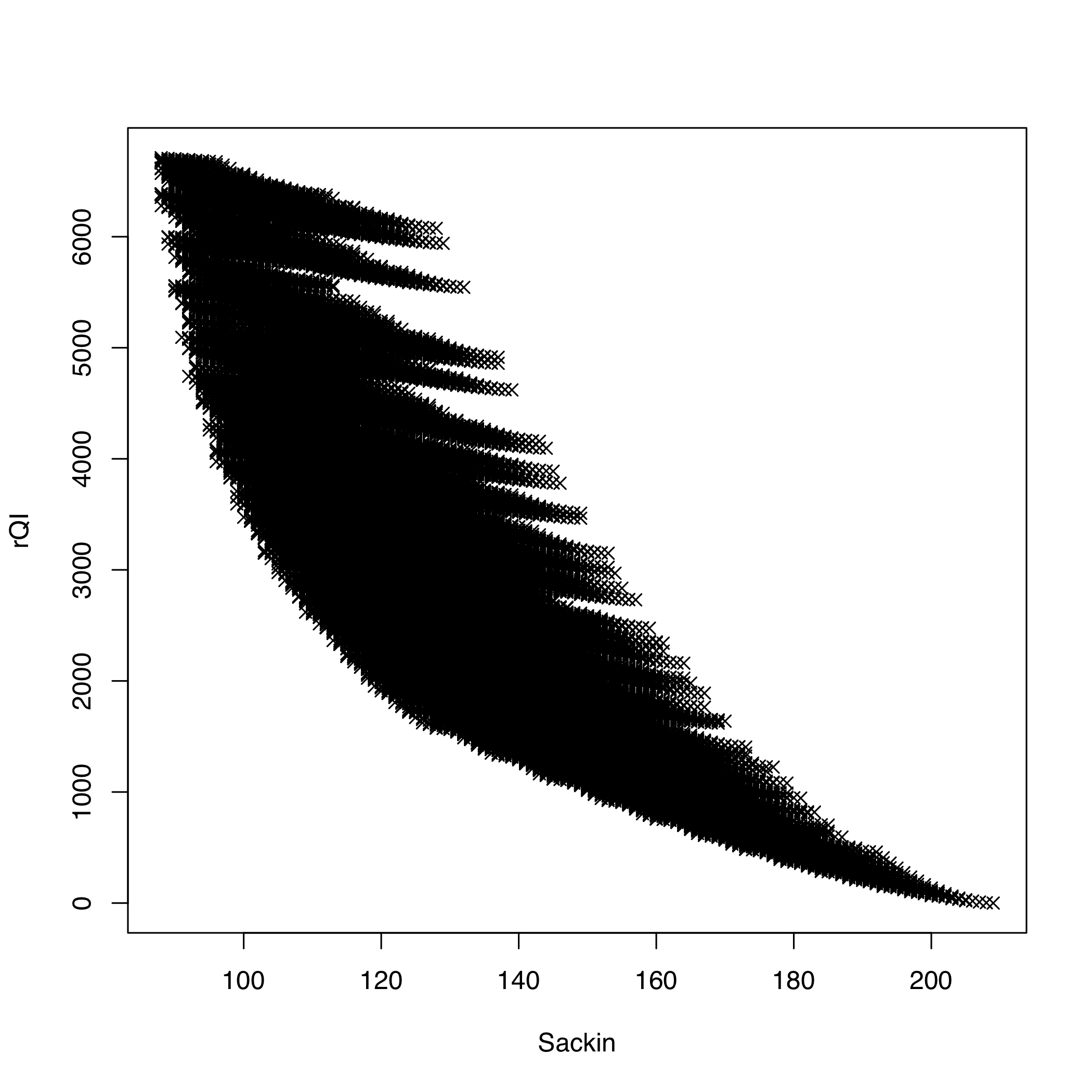
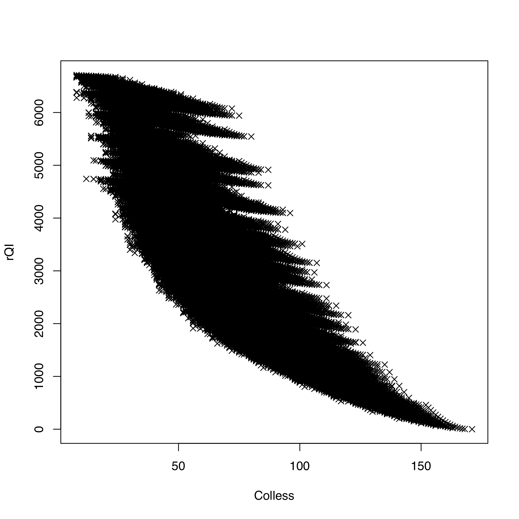
(a)	(b)
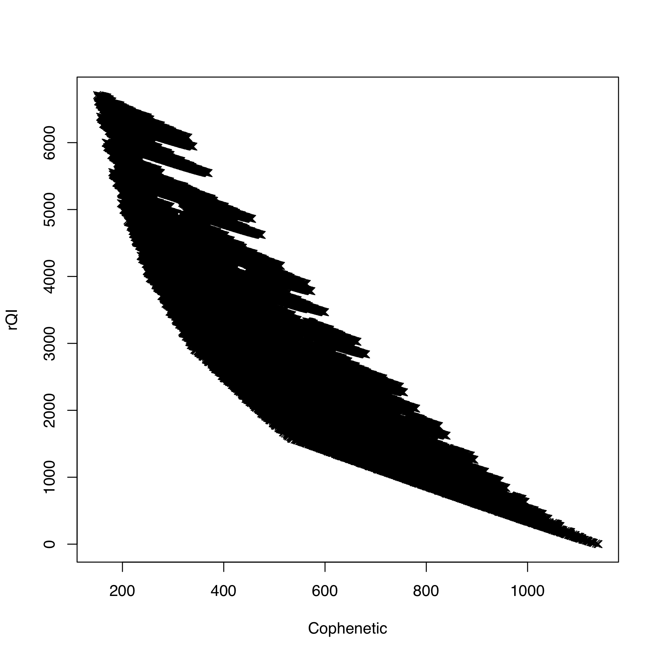
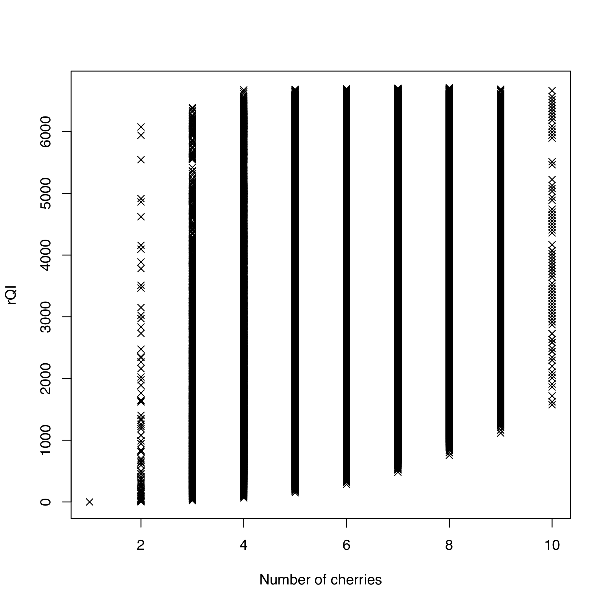
(c)	(d)
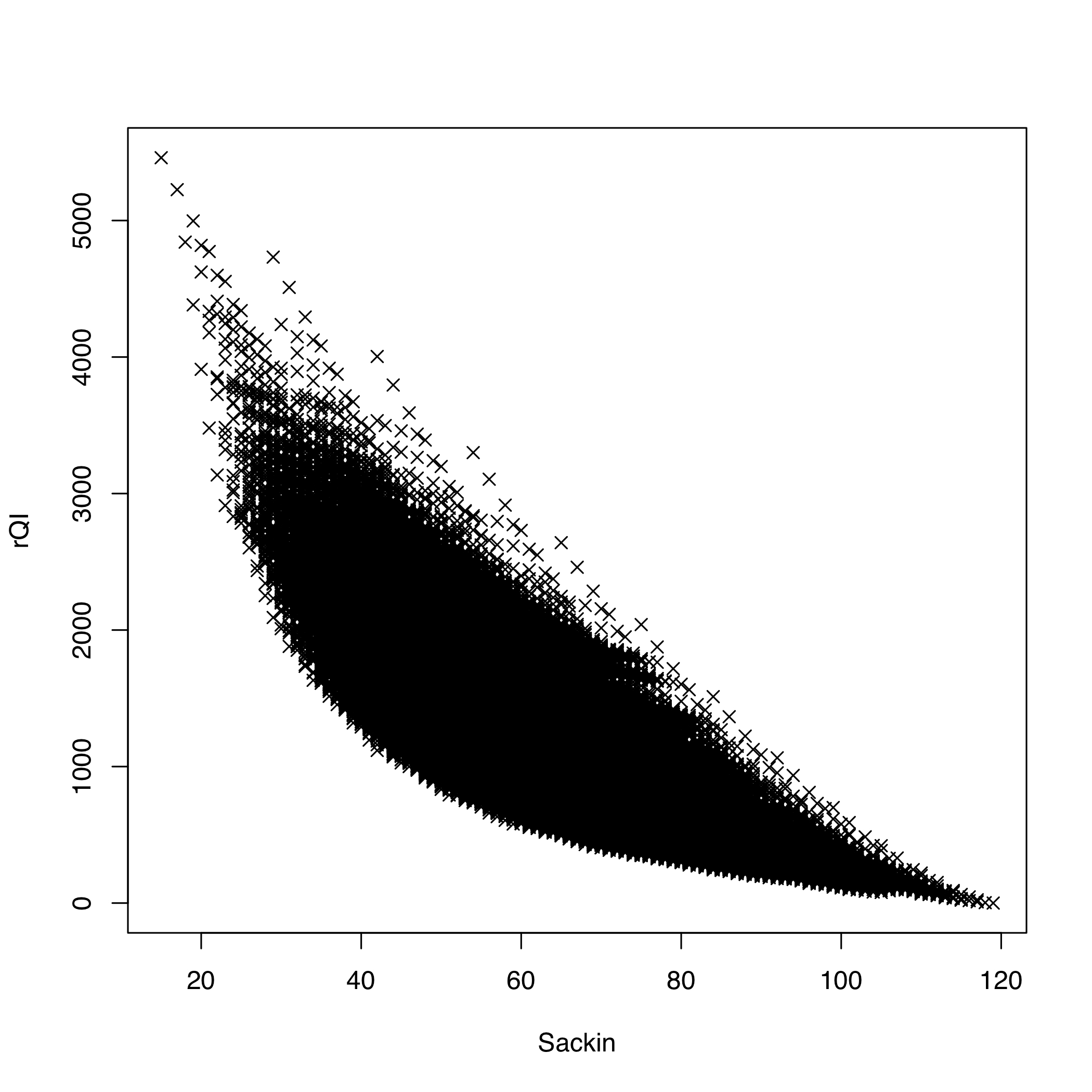
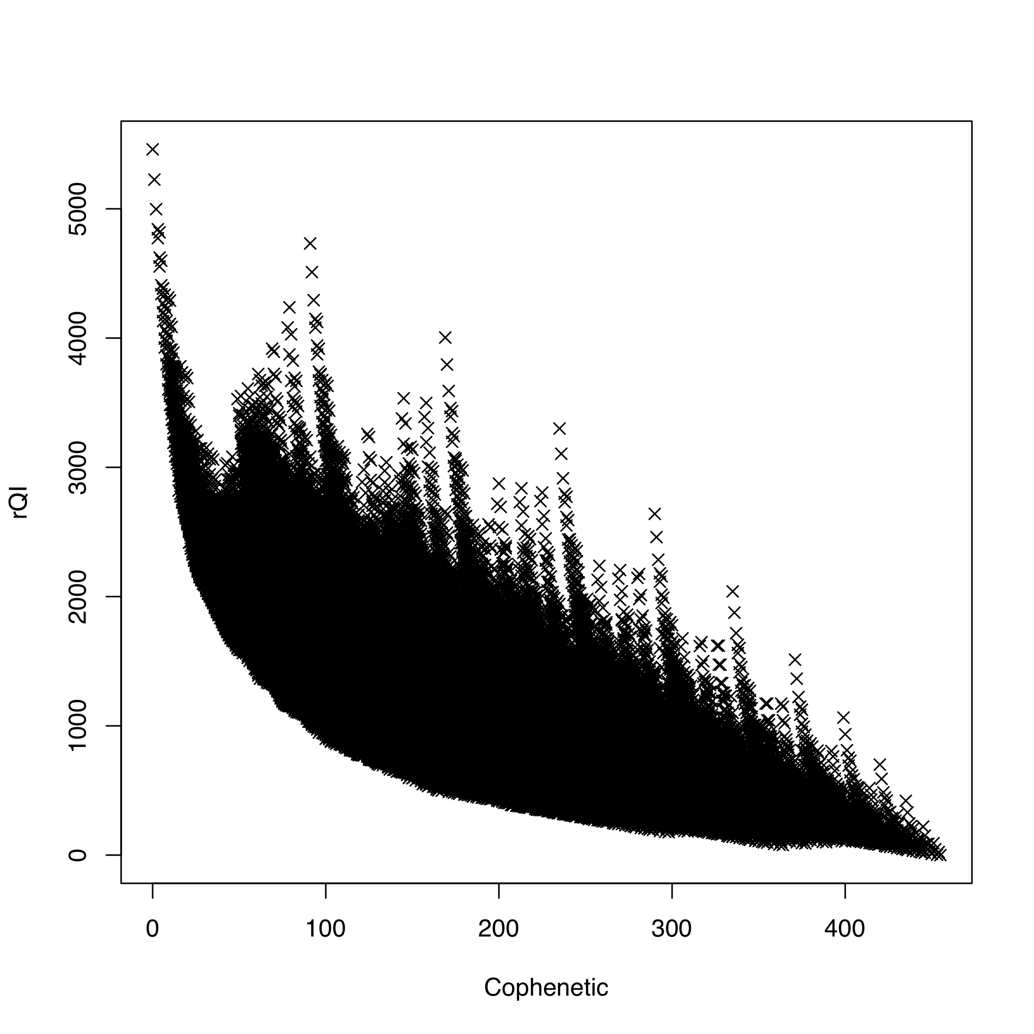
(e)	(f)

Figure 12: Scatterplot of $\mathit{rQI}$ versus: (a) the Sackin index on $\mathcal{BT\!}_{20}$; (b) the Colless index on $\mathcal{BT\!}_{20}$; (c) the total cophenetic index on $\mathcal{BT\!}_{20}$; (d) the number of cherries on $\mathcal{BT\!}_{20}$; (e) the Sackin index on $\mathcal{T}_{15}$; (f) the total cophenetic index on $\mathcal{T}_{15}$.

Correlation	Value
$\mathit{rQI}$ vs $S$ on $\mathcal{BT\!}_{20}$	$-0.889$
$\mathit{rQI}$ vs $C$ on $\mathcal{BT\!}_{20}$	$-0.893$
$\mathit{rQI}$ vs $\Phi$ on $\mathcal{BT\!}_{20}$	$-0.935$
$\mathit{rQI}$ vs $\mathit{Ch}$ on $\mathcal{BT\!}_{20}$	$0.165$
$\mathit{rQI}$ vs $S$ on $\mathcal{T}_{15}$	$-0.787$
$\mathit{rQI}$ vs $\Phi$ on $\mathcal{T}_{15}$	$-0.827$

Table 2: Spearman’s correlations corresponding to the scatterplots in Fig. 12.

Acknowledgements. A preliminary version of this paper was presented at the Workshop on Algebraic and combinatorial phylogenetics held in Barcelona (June 26–30, 2017). We thank Mike Steel, Gabriel Riera, Seth Sullivant, the anonymous reviewers and the associate editor for their helpful suggestions on several aspects of this paper. This research was partially supported by the Spanish Ministry of Economy and Competitiveness and the European Regional Development Fund through project DPI2015-67082-P (MINECO /FEDER).

Appendices

A.1: An alternative derivation of the variance of $\mathit{rQIB}_{n}$ under the Yule model

In this section we give an alternative proof of the following result.

Proposition 29.

Under the Yule model,

$$Var_{Y}(\mathit{rQIB}_{n})=\binom{n}{4}\frac{5n^{4}+30n^{3}+118n^{2}+408n+630}{33075}.$$

Proof.

By Lemma 10, $\mathit{rQIB}$ on $\mathcal{BT\!}_{n}$ is a bifurcating recursive tree shape statistic satisfying the recurrence

$$\mathit{rQIB}(T\star T^{\prime})=\mathit{rQIB}(T)+\mathit{rQIB}(T^{\prime})+f_{\mathit{rQIB}}(|L(T)|,|L(T^{\prime})|)$$

with $f_{\mathit{rQIB}}(a,b)=\binom{a}{2}\binom{b}{2}$. Then, it satisfies the hypothesis in Cor. 1 of [5] with

$$\begin{array}[]{rl}\displaystyle\varepsilon(a,b-1)&\displaystyle=f_{\mathit{rQIB}}(a,b)-f_{\mathit{rQIB}}(a,b-1)\\ &\displaystyle=\binom{a}{2}\binom{b}{2}-\binom{a}{2}\binom{b-1}{2}=(b-1)\binom{a}{2}\\[8.61108pt] \displaystyle R(n-1)&\displaystyle=E_{Y}(\mathit{rQIB}_{n})-E_{Y}(\mathit{rQIB}_{n-1})\\ &\displaystyle=\frac{1}{3}\binom{n}{4}-\frac{1}{3}\binom{n-1}{4}=\frac{1}{3}\binom{n-1}{3}\end{array}$$

Since $E_{Y}(\mathit{rQIB}_{1})=0$ and $f_{\mathit{rQIB}}(n-1,1)=0$, applying the aforementioned result from [5] we have that

$$\begin{array}[]{l}E_{Y}(\mathit{rQIB}_{n}^{2})\displaystyle=\frac{n}{n-1}E_{Y}(\mathit{rQIB}_{n-1}^{2})+\frac{4}{n-1}\sum_{k=1}^{n-2}\varepsilon(k,n-k-1)E_{Y}(\mathit{rQIB}_{k})\\ \qquad\qquad\displaystyle+\frac{2}{n-1}\sum_{k=1}^{n-2}R(n-k-1)E_{Y}(\mathit{rQIB}_{k})\\ \qquad\qquad\displaystyle+\frac{1}{n-1}\sum_{k=1}^{n-2}(f_{\mathit{rQIB}}(k,n-k)^{2}-f_{\mathit{rQIB}}(k,n-k-1)^{2})\\[8.61108pt] \qquad\displaystyle=\frac{n}{n-1}E_{Y}(\mathit{rQIB}_{n-1}^{2})+\frac{4}{3(n-1)}\sum_{k=1}^{n-2}(n-k-1)\binom{k}{2}\binom{k}{4}\\ \qquad\qquad\displaystyle+\frac{2}{9(n-1)}\sum_{k=1}^{n-2}\binom{n-k-1}{3}\binom{k}{4}\\ \qquad\qquad\displaystyle+\frac{1}{n-1}\sum_{k=1}^{n-2}\binom{k}{2}^{2}\Bigg{(}\binom{n-k}{2}^{2}-\binom{n-k-1}{2}^{2}\Bigg{)}\\[8.61108pt] \qquad\displaystyle=\frac{n}{n-1}E_{Y}(\mathit{rQIB}_{n-1}^{2})+\frac{n}{3}\binom{n-2}{4}\frac{15n^{2}-35n+6}{420}\\[4.30554pt] \qquad\qquad\displaystyle+\frac{n}{9}\binom{n-2}{4}\frac{n^{2}-13n+42}{840}\\[4.30554pt] \qquad\qquad\displaystyle+n\binom{n-2}{2}\frac{3n^{4}-18n^{3}+41n^{2}-42n+36}{1680}\\[8.61108pt] \qquad\displaystyle=\frac{n}{n-1}E_{Y}(\mathit{rQIB}_{n-1}^{2})\\[4.30554pt] \qquad\qquad\displaystyle+\frac{n(n-2)(n-3)(253n^{4}-2014n^{3}+6119n^{2}-7430n+3504)}{181440}\end{array}$$

Dividing by $n$ both sides of this expression for $E_{Y}(\mathit{rQIB}^{2}_{n})$ and setting $y_{n}=E_{Y}(\mathit{rQIB}^{2}_{n})/n$, we obtain the recurrence

$$\begin{array}[]{rl}y_{n}&=\displaystyle y_{n-1}+\frac{(n-2)(n-3)(253n^{4}-2014n^{3}+6119n^{2}-7430n+3504)}{181440}.\end{array}$$

Since $y_{0}=y_{1}=0$, its solution is

$$\begin{array}[]{rl}y_{n}&\displaystyle=\sum_{k=2}^{n}\frac{(k-2)(k-3)(253k^{4}-2014k^{3}+6119k^{2}-7430k+3504)}{181440}\\[4.30554pt] &\displaystyle=\frac{(n-3)(n-2)(n-1)(1265n^{4}-7110n^{3}+14419n^{2}-4086n+5040)}{6350400}\end{array}$$

from where we obtain

$$\begin{array}[]{rl}E_{Y}(\mathit{rQIB}_{n}^{2})&=ny_{n}\\ &\displaystyle=\binom{n}{4}\frac{1265n^{4}-7110n^{3}+14419n^{2}-4086n+5040}{264600}.\end{array}$$

Finally

$$\begin{array}[]{l}Var_{Y}(\mathit{rQIB}_{n})\displaystyle=E_{Y}(\mathit{rQIB}_{n}^{2})-E_{Y}(\mathit{rQIB}_{n})^{2}\\ \qquad\displaystyle=\binom{n}{4}\frac{1265n^{4}-7110n^{3}+14419n^{2}-4086n+5040}{264600}-\frac{1}{9}\binom{n}{4}^{2}\\ \qquad\displaystyle=\binom{n}{4}\frac{5n^{4}+30n^{3}+118n^{2}+408n+630}{33075},\end{array}$$

as we claimed. ∎∎

A.2: Some tables used in Section 5

Name	Shape	$\Theta_{3,3}(T^{*})$
$B_{5,1}^{*}$	$(*,(*,(*,(*,*))))$	0
$B_{5,2}^{*}$	$(*,((*,*),(*,*)))$	0
$B_{5,3}^{*}$	$((*,*),(*,(*,*)))$	6
$B_{6,1}^{*}$	$(*,(*,(*,(*,(*,*)))))$	0
$B_{6,2}^{*}$	$(*,(*,((*,*),(*,*))))$	0
$B_{6,3}^{*}$	$(*,((*,*),(*,(*,*))))$	0
$B_{6,4}^{*}$	$((*,*),((*,*),(*,*)))$	18
$B_{6,5}^{*}$	$((*,*),(*,(*,(*,*))))$	6
$B_{6,6}^{*}$	$((*,(*,*)),(*,(*,*)))$	36
$B_{7,1}^{*}$	$(*,(*,(*,(*,(*,(*,*))))))$	0
$B_{7,2}^{*}$	$(*,(*,(*,((*,*),(*,*)))))$	0
$B_{7,3}^{*}$	$(*,(*,((*,*),(*,(*,*)))))$	0
$B_{7,4}^{*}$	$(*,((*,*),((*,*),(*,*))))$	0
$B_{7,5}^{*}$	$(*,((*,*),(*,(*,(*,*)))))$	0
$B_{7,6}^{*}$	$(*,((*,(*,*)),(*,(*,*))))$	0
$B_{7,7}^{*}$	$((*,*),(*,(*,(*,(*,*)))))$	0
$B_{7,8}^{*}$	$((*,*),(*,((*,*),(*,*))))$	8
$B_{7,9}^{*}$	$((*,*),((*,*),(*,(*,*))))$	24
$B_{7,10}^{*}$	$((*,(*,*)),(*,(*,(*,*))))$	36
$B_{7,11}^{*}$	$((*,(*,*)),((*,*),(*,*)))$	36
$B_{8,1}^{*}$	$(*,(*,(*,(*,(*,(*,(*,*)))))))$	0
$B_{8,2}^{*}$	$(*,(*,(*,(*,((*,*),(*,*))))))$	0
$B_{8,3}^{*}$	$(*,(*,(*,((*,*),(*,(*,*))))))$	0
$B_{8,4}^{*}$	$(*,(*,((*,*),((*,*),(*,*)))))$	0
$B_{8,5}^{*}$	$(*,(*,((*,*),(*,(*,(*,*))))))$	0
$B_{8,6}^{*}$	$(*,(*,((*,(*,*)),(*,(*,*)))))$	0
$B_{8,7}^{*}$	$(*,((*,*),(*,(*,(*,(*,*))))))$	0
$B_{8,8}^{*}$	$(*,((*,*),(*,*),(*,(*,*)))))$	0
$B_{8,9}^{*}$	$(*,((*,*),(*,((*,*),(*,*)))))$	0
$B_{8,10}^{*}$	$(*,((*,(*,*)),(*,(*,(*,*)))))$	0
$B_{8,11}^{*}$	$(*,((*,(*,*)),((*,*),(*,*))))$	0
$B_{8,12}^{*}$	$((*,*),(*,(*,(*,(*,(*,*))))))$	0
$B_{8,13}^{*}$	$((*,*),(*,(*,(*,*),(*,*))))$	2
$B_{8,14}^{*}$	$((*,*),(*,((*,*),(*,(*,*)))))$	6
$B_{8,15}^{*}$	$((*,*),((*,*),(*,(*,(*,*))))))$	12
$B_{8,16}^{*}$	$((*,*),((*,*),((*,*),(*,*))))$	14
$B_{8,17}^{*}$	$((*,*),((*,(*,*)),(*,(*,*))))$	18
$B_{8,18}^{*}$	$((*,(*,*)),(*,(*,(*,(*,*)))))$	0
$B_{8,19}^{*}$	$((*,(*,*)),(*,((*,*),(*,*)))))$	0
$B_{8,20}^{*}$	$((*,(*,*)),((*,*),(*,(*,*))))$	0
$B_{8,21}^{*}$	$((*,(*,(*,*))),(*,(*,(*,*))))$	36
$B_{8,22}^{*}$	$((*,(*,(*,*))),((*,*),(*,*)))$	36
$B_{8,23}^{*}$	$(((*,*),(*,*)),((*,*),(*,*)))$	38

Table 3: Coefficients of the probabilities of the trees in $\mathcal{BT\!}_{k}^{*}$, for $k=5,6,7,8$, in the formula for the variance of $\mathit{rQIB}_{n}$.

Tree	$P_{\alpha,n}^{A,*}$
$\Big{(}$ $Q_{3}^{*}$	$\frac{1-\alpha}{3-\alpha}$
$\Big{(}$ $B_{5,3}^{*}$	$\frac{2(1-\alpha)}{4-\alpha}$
$\Big{(}$ $B_{6,4}^{*}$	$\frac{(1-\alpha)^{2}(8-\alpha)}{(5-\alpha)(4-\alpha)(3-\alpha)}$
$\Big{(}$ $B_{6,5}^{*}$	$\frac{2(1-\alpha)(8-\alpha)}{(5-\alpha)(4-\alpha)(3-\alpha)}$
$\Big{(}$ $B_{6,6}^{*}$	$\frac{2(1-\alpha)(2-\alpha)}{(5-\alpha)(4-\alpha)}$
$\Big{(}$ $B_{7,8}^{*}$	$\frac{(1-\alpha)^{2}(2+\alpha)(10+\alpha)}{(6-\alpha)(5-\alpha)(4-\alpha)(3-\alpha)}$
$\Big{(}$ $B_{7,9}^{*}$	$\frac{2(1-\alpha)^{2}(10+\alpha)}{(6-\alpha)(5-\alpha)(4-\alpha)}$
$\Big{(}$ $B_{7,10}^{*}$	$\frac{10(1-\alpha)(2-\alpha)}{(6-\alpha)(5-\alpha)(3-\alpha)}$
$\Big{(}$ $B_{7,11}^{*}$	$\frac{5(1-\alpha)^{2}(2-\alpha)}{(6-\alpha)(5-\alpha)(3-\alpha)}$
$\Big{(}$ $B_{8,13}^{*}$	$\frac{8(1-\alpha)^{2}(1+\alpha)(2+\alpha)(3+\alpha)}{(7-\alpha)(6-\alpha)(5-\alpha)(4-\alpha)(3-\alpha)}$
$\Big{(}$ $B_{8,14}^{*}$	$\frac{16(1-\alpha)^{2}(1+\alpha)(3+\alpha)}{(7-\alpha)(6-\alpha)(5-\alpha)(4-\alpha)}$
$\Big{(}$ $\Big{(}$ $B_{8,15}^{*}$	$\frac{8(1-\alpha)^{2}(3+\alpha)(8-\alpha)}{(7-\alpha)(6-\alpha)(5-\alpha)(4-\alpha)(3-\alpha)}$
$\Big{(}$ $B_{8,16}^{*}$	$\frac{4(1-\alpha)^{3}(3+\alpha)(8-\alpha)}{(7-\alpha)(6-\alpha)(5-\alpha)(4-\alpha)(3-\alpha)}$
$\Big{(}$ $B_{8,17}^{*}$	$\frac{8(1-\alpha)^{2}(2-\alpha)(3+\alpha)}{(7-\alpha)(6-\alpha)(5-\alpha)(4-\alpha)}$
$\Big{(}$ $B_{8,21}^{*}$	$\frac{20(1-\alpha)(2-\alpha)}{(7-\alpha)(6-\alpha)(5-\alpha)(3-\alpha)}$
$\Big{(}$ $B_{8,22}^{*}$	$\frac{20(1-\alpha)^{2}(2-\alpha)}{(7-\alpha)(6-\alpha)(5-\alpha)(3-\alpha)}$
$\Big{(}$ $B_{8,23}^{*}$	$\frac{5(1-\alpha)^{3}(2-\alpha)}{(7-\alpha)(6-\alpha)(5-\alpha)(3-\alpha)}$

Table 4: Probabilities under the $\alpha$-model of the trees involved in the formula for the variance of $\mathit{rQIB}_{n}$

Tree	$P_{\beta,n}^{B,*}$
$\Big{(}$ $Q_{3}^{*}$	$\frac{3(\beta+2)}{7\beta+18}$
$\Big{(}$ $B_{5,3}^{*}$	$\frac{2(\beta+2)}{3\beta+8}$
$\Big{(}$ $B_{6,4}^{*}$	$\frac{45(\beta+2)^{2}(\beta+4)}{(31\beta^{2}+194\beta+300)(7\beta+18)}$
$\Big{(}$ $B_{6,5}^{*}$	$\frac{60(\beta+2)(\beta+3)(\beta+4)}{(31\beta^{2}+194\beta+300)(7\beta+18)}$
$\Big{(}$ $B_{6,6}^{*}$	$\frac{10(\beta+2)(\beta+3)}{31\beta^{2}+194\beta+300}$
$\Big{(}$ $B_{7,8}^{*}$	$\frac{3(\beta+2)^{2}(\beta+4)(\beta+5)}{(\beta+3)(3\beta+8)(3\beta+10)(7\beta+18)}$
$\Big{(}$ $B_{7,9}^{*}$	$\frac{2(\beta+2)^{2}(\beta+5)}{(\beta+3)(3\beta+8)(3\beta+10)}$
$\Big{(}$ $B_{7,10}^{*}$	$\frac{20(\beta+2)(\beta+3)}{3(3\beta+10)(7\beta+18)}$
$\Big{(}$ $B_{7,11}^{*}$	$\frac{5(\beta+2)^{2}}{(3\beta+10)(7\beta+18)}$
$\Big{(}$ $B_{8,13}^{*}$	$\frac{504(\beta+2)^{2}(\beta+4)^{2}(\beta+5)^{2}(\beta+6)}{(127\beta^{3}+1383\beta^{2}+4958\beta+5880)(31\beta^{2}+194\beta+300)(3\beta+8)(7\beta+18)}$
$\Big{(}$ $B_{8,14}^{*}$	$\frac{336(\beta+2)^{2}(\beta+4)(\beta+5)^{2}(\beta+6)}{(127\beta^{3}+1383\beta^{2}+4958\beta+5880)(31\beta^{2}+194\beta+300)(3\beta+8)}$
$\Big{(}$ $B_{8,15}^{*}$	$\frac{1680(\beta+2)^{2}(\beta+3)(\beta+4)(\beta+5)(\beta+6)}{(127\beta^{3}+1383\beta^{2}+4958\beta+5880)(31\beta^{2}+194\beta+300)(7\beta+18)}$
$\Big{(}$ $B_{8,16}^{*}$	$\frac{1260(\beta+2)^{3}(\beta+4)(\beta+5)(\beta+6)}{(127\beta^{3}+1383\beta^{2}+4958\beta+5880)(31\beta^{2}+194\beta+300)(7\beta+18)}$
$\Big{(}$ $B_{8,17}^{*}$	$\frac{280(\beta+2)^{2}(\beta+3)(\beta+5)(\beta+6)}{(127\beta^{3}+1383\beta^{2}+4958\beta+5880)(31\beta^{2}+194\beta+300)}$
$\Big{(}$ $B_{8,21}^{*}$	$\frac{560(\beta+2)(\beta+3)^{3}(\beta+4)}{(127\beta^{3}+1383\beta^{2}+4958\beta+5880)(7\beta+18)^{2}}$
$\Big{(}$ $B_{8,22}^{*}$	$\frac{840(\beta+2)^{2}(\beta+3)^{2}(\beta+4)}{(127\beta^{3}+1383\beta^{2}+4958\beta+5880)(7\beta+18)^{2}}$
$\Big{(}$ $B_{8,23}^{*}$	$\frac{315(\beta+2)^{3}(\beta+3)(\beta+4)}{(127\beta^{3}+1383\beta^{2}+4958\beta+5880)(7\beta+18)^{2}}$

Table 5: Probabilities under the $\beta$-model of the trees involved in the formula for the variance of $\mathit{rQIB}_{n}$

References

• Abramowitz and Stegun [1972] Abramowitz M, Stegun IAS (1972) Handbook of Mathematical Functions with Formulas, Graphs, and Mathematical Tables. Dover
• Aldous [1996] Aldous D (1996) Probability distributions on cladograms. In: Random discrete structures, The IMA Voumes in Mathematics and its Applications, vol 76, Springer, pp 1–18
• Aldous [2001] Aldous D (2001) Stochastic models and descriptive statistics for phylogenetic trees, from Yule to today. Statistical Science 16:23–34
• Blum and François [2005] Blum MGB, François OF (2005) On statistical tests of phylogenetic tree imbalance: The Sackin and other indices revisited. Mathematical Biosciences 195:141–153
• Cardona et al [2013] Cardona G, Mir A, Rosselló F (2013) Exact formulas for the variance of several balance indices under the Yule model. Journal of Mathematical Biology 67:1833–1846
• Cavalli-Sforza and Edwards [1967] Cavalli-Sforza LL, Edwards A (1967) Phylogenetic analysis: Models and estimation procedures. Evolution 21:550–570
• Chen et al [2009] Chen B, Ford D, Winkel M (2009) A new family of Markov branching trees: the alpha-gamma model. Electronic Journal of Probability 14:400–430
• Colless [1982] Colless DH (1982) Review of “Phylogenetics: The theory and practice of phylogenetic systematics”. Systematic Zoology 31:100–104
• Cormen et al [2009] Cormen TH, Leiserson CE, Rivest RL, Stein C (2009) Introduction to Algorithms (3rd edition). The MIT Press
• Coronado et al [2018] Coronado TM, Mir A, Rosselló F (2018) The probabilities of trees and cladograms under Ford’s $\alpha$-model. The Scientific World Journal 2018:1916094
• Dearlove and Frost [2015] Dearlove BL, Frost SD (2015) Measuring asymmetry in time-stamped phylogenies. PLoS Computational Biology 11.7 (2015):e1004312
• Felsenstein [2004] Felsenstein J (2004) Inferring Phylogenies. Sinauer Associates Inc
• Ford [2005] Ford D (2005) Probabilities on cladograms: Introduction to the alpha model. arXiv preprint math/0511246
• Harding [1971] Harding E (1971) The probabilities of rooted tree-shapes generated by random bifurcation. Advances in Applied Probility 3:44–77
• Keller-Schmidt et al [2015] Keller-Schmidt S, Tuğrul M, Eguíluz VM, Hernández-García E, Klemm K (2015) Anomalous scaling in an age-dependent branching model. Physical Review E 91:022803
• Kirkpatrick and Slatkin [1993] Kirkpatrick M, Slatkin M (1993) Searching for evolutionary patterns in the shape of a phylogenetic tree. Evolution 47:1171–1181
• Macdonald [1995] Macdonald IG (1995) Symmetric functions and Hall polynomials (2nd edition). Oxford University Press
• Matsen [2007] Matsen F (2007) Optimization over a class of tree shape statistics. IEEE/ACM Transactions on Computational Biology and Bioinformatics (TCBB) 4:506–512
• Steel and McKenzie [2000] McKenzie A, Steel M (2000) Distributions of cherries for two models of trees. Mathematical Biosciences 164:81–92
• Mir et al [2013] Mir A, Rosselló F, Rotger L (2013) A new balance index for phylogenetic trees. Mathematical Biosciences 241:125–136
• Mir et al [2018] Mir A, Rotger L, Rosselló F (2018) Sound Colless-like balance indices for multifurcating trees. PLoS ONE 13(9):e0203401
• Mooers and Heard [1997] Mooers A, Heard SB (1997) Inferring evolutionary process from phylogenetic tree shape. The Quarterly Review of Biology 72:31–54
• Pinelis [2003] Pinelis I (2003) Evolutionary models of phylogenetic trees. Proceedings of the Royal Society of London B: Biological Sciences 270:1425–1431
• Rosen [1978] Rosen DE (1978) Vicariant patterns and historical explanation in biogeography. Systematic Biology 27:159–188
• Sackin [1972] Sackin MJ (1972) Good and “bad” phenograms. Systematic Zoology 21:225–226
• Shao and Sokal [1990] Shao KT, Sokal R (1990) Tree balance. Systematic Zoology 39:226–276
• Sloane [2010] Sloane NJA (2010) The On-Line Encyclopedia of Integer Sequences. URL http://oeis.org/
• Wu and Choi [2016] Wu T, Choi, KP (2016) On joint subtree distributions under two evolutionary models. Theoretical Population Biology, 108:13-23
• Yule [1924] Yule GU (1924) A mathematical theory of evolution based on the conclusions of Dr J. C. Willis. Philosophical Transactions of the Royal Society of London Series B 213:21–87
• Zhu, Degnan and Steel [2011] Zhu S, Degnan JH, Steel M (2011) Clades, clans and reciprocal monophyly under neutral evolutionary models. Theoretical Population Biology 79:220–227
• Zhu, Than and Wu [2015] Zhu S, Than C, Wu T (2015) Clades and clans: a comparison study of two evolutionary models. Journal of Mathematical Biology, 71:99–124