Dynamics of a system of coupled inverted pendula with vertical forcing

Abstract

Dynamical stabilization of an inverted pendulum through vertical movement of the pivot is a well-known counter intuitive phenomenon in classical mechanics. This system is also known as Kapitza pendulum and the stability can be explained with the aid of effective potential. We explore the effect of many body interaction for such a system. Our numerical analysis shows that interaction between pendula generally degrades the dynamical stability of each pendulum. This effect is more pronounced in nearest neighbour coupling than all-to-all coupling and stability improves with the increase of the system size. We report development of beats and clustering in network of coupled pendula.

1 Introduction

An ordinary rigid planar pendulum with a fixed suspension point has only one stable configuration, the bob hanging below the suspension point. However, if a vertical periodic force is applied at the suspension point, the system becomes stable in the vertical position also, provided the amplitude and the frequency are kept within certain intervals. This is an example of dynamic stabilization and has several applications in the field of atomic physics Paul1990 ; Gilary2003 , plasma physics Bullo2002 and cybernetics Nakamura1997 . This unusual and counterintuitive phenomenon was first experimentally observed by Stephenson Stephenson1908 and theoretically explained by P. Kapitza Haar(Eds.)1965 . The system is also known as Kapitza pendulum. There exists a large volume of literature in this field, both experimental and theoretical Kim1998 ; Butikov2001 ; Broer1999 ; Broer2004 ; Bartuccelli2001 ; Bartuccelli2002 ; Bartuccelli2003 . The potential function is time dependent which leads to dynamic stabilization.

What happens when such systems interact with each other? What is the effect of coupling in such a system with spatio-temporal potential? Of late, the understanding of periodically driven systems has become one of the most active areas of research in many body physics. In the context of spatiotemporal chaos, coupled Kapitza pendulum in a dissipative environment has been investigated in Chacon2010 . Ref.Marcheggiani2014 addresses the issue of synchronization in a coupled Kapitza pendulum where the coupling is mechanically linear and geometrically nonlinear. Parametric oscillator in several contexts has been rigorously investigated in previous works Moehlis2008 ; Danzl2010 ; Xu2014 ; SalgadoSanchez2016 .

In this work, we specifically address the effect on the stability range around the inverted position due to the presence of interaction between pendula. A recent work by Citro et al. Citro2015 addressed this question in a network of pendula with nearest neighbour coupling. The coupled Kapitza pendula in the continuum limit is shown to take the form of a periodically-driven Sine-Gordon model. If interaction is introduced, the stabilization property changes which is characterised by the interaction strength. In recent times, the study of periodically driven many body systems has drawn attention due to the recent advancement in the field of ultra-cold atoms Eckardt2005 ; Lignier2007 ; Struck2011 ; Struck2012 .

It is often assumed that a many-body system undergoing a cyclic process will reach infinite temperature as demanded by the second law of thermodynamics. But several research works have shown that periodic heating and cooling is possible in such a system Russomanno2012 ; Ponte2015 ; Ponte2015a . Apperance of parametric resonance can explain this phenomenon by separating the absorbing and non-absorbing regimes. Such interactions have so far been considered only in a 1-D chain. Do the same result hold in a 2D lattice? What is the effect of system size(the number of interacting pendula)?

The effect of long range interaction has not been addressed in these works. Moreover, the effect of nearest neighbor coupling has been studied only in a 1D chain. We study the effect of all to all interaction in our present work and compare with the result of the 1D case. We have investigated the effect of the nearest neighbour interaction in a 2D network as well.

The dynamics of the particle system with all to all interaction i.e., long range interaction offers several unusual and new characteristics in comparison with systems with short-range or nearest neighbour interactions. The Kuramoto oscillator and the Hamiltonian mean field model are two iconic test-beds for such class of systems. This kind of long range interaction demands statistical treatment. The state of the art method to deal with this class of problems is the mean field theory (MFT), where all the interactions are considered to be of equal strength. Through the mean field treatment the complexity of the system reduces drastically. In this work, we use numerical simulations to study the coupled pendulum system with all to all interaction. Our attempt is to find the stability regime for the system and dynamics of the coupled system. We numerically obtain the maximum release angle beyond which the stabilization of the inverted state is not achievable.

We also obtain how this maximum release angle, which is a measure of the stability of the system, changes with the size of the system $N$ and the type of coupling. We consider three different cases for the coupled system. Our study includes nearest neighbour interaction as well as all to all interaction. To observe the effect of dimension we investigate a 2D square network. Finite size effect, i.e., dependence of stability on the total number of pendula has also been discussed in this context.

The paper is organized as follows. In Sec. 2 we briefly recall the single Kapitza pendulum and its stability condition. In Sec. 3 we consider many body interaction of different types. We present some concluding remarks in Sec. 4.

2 Single Kapitza pendulum

Here we briefly summarize the case of a single inverted pendulum where the pivot oscillates vertically with amplitude $g_{1}$ and frequency $\omega$ (Fig.1). The Hamiltonian governing the system is

$$H=\frac{p^{2}}{2}-g(t)\cos{\phi},$$ (1)

Figure 1: Schematic diagram of single, isolated Kapitza pendulum. O is the point of suspension subject to a high frequency vertical drive $y=g_{1}\cos{\omega t}$. $\phi$ represents the angular dispacement.

where $p$ and $\phi$ are momentum and angular displacement of the pendulum respectively and $g(t)=g_{0}+g_{1}\cos{\omega t}$. When the vertical drive is absent i.e., $g_{1}=0$, there are two fixed points $\phi=0$ (stable) and $\phi=\pi$ (unstable). If $g_{1}\neq 0$, the inverted position i.e., $\phi=\pi$ configuration can be stable if $\omega$ is very high compared to the natural frequency $\sqrt{g_{0}}$ . In order to understand the stable configuration for this time dependent potential system an effective potential is required to be calculated which was for the first time obtained by Kapitza by separating the ‘fast’ and ‘slow’ variables and integrating out the ‘fast’ ones. The condition for stabilization of the inverted position turned out to be $g_{1}^{2}\geq g_{0}\omega^{2}/2$. This concept of effective potential gave birth to a new branch of physics, named dynamical stabilization. The method to obtain the effective potential for such a system is perturbative and the result is approximate. One can obtain the exact trajectory only through numerical analysis.

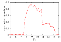
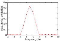
(a)    (b)

Figure 2: Stability of a single Kapitza pendulum: the maximum initial deviation from the inverted position $\phi=\pi$ for stability (a) for different values of applied amplitude $g_{1}$, with $g_{0}=1,\omega=5$, (b) for different values of applied frequency $\omega$ with $g_{0}=1,g_{1}=10$.

From the effective potential, we obtain the shape of the potential well. It can be shown that if the driving frequency is fixed at some value and the amplitude of the drive is increased, the well becomes wider Blackburn1992 . The maximum initial displacement for stabilization of the inverted pendulum quantifies the extent of dynamical stabilization for the system. We compute the maximum release angle beyond which the stabilization at the inverted position is lost for the system. This is a measure of the stability region around the inverted position of this system. Fig.2(a) shows how the maximum initial angle changes as we change the parameter $g_{1}$. This probes the width of the potential well for the system. Fig.2(b) represents the stability regime as the frequency of the drive is changed. These two figures show that, in case of the single Kapitza pendulum, there exists a range of initial deviation from the vertical position for which the inverted position is stable, and that this range is maximum at specific values of $g_{1}$ and $\omega$.

To compute the numerical solutions a $4^{\rm th}$ order Runge Kutta method was employed, with time step $0.01$ times the period of the drive ($\frac{2\pi}{\omega}$). Now we explore how these ranges are affected when multiple Kapitza pendula interact with each other.

3 Many body Kapitza pendula

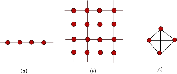
Figure 3: Schematic diagram of the coupled inverted pendulum. (a) 1D pendulum chain with nn uniform coupling (b) 2D pendulum network with nn coupling (c) Pendulum network with all to all coupling.

Now we study the stability of Kapitza pendula when more than one body is involved. We observe several departures from the single particle dynamics of this system. In this work, we explore three cases:

1. nearest neighbour (nn) interaction in a 1D pendulum chain,

2. 2D pendulum chain with nn interaction, and

3. coupled system with all-to-all interaction.

We assume uniform coupling in all these three cases. These three cases can be demonstrated in the form of three different lattice structures where each lattice point represents the bob of an inverted pendulum (Fig. 3). For example, in the square lattice of Fig. 3(b), each point is the pendulum bob and each one is connected to its nearest neighbour, i.e., every pendulum is connected to its four neighbour pendula.

To observe the effect of this interaction between the pendula we introduce a parameter $\Lambda$ into the Hamiltonian, which is a measure of relative strength of the interaction between the pendula and the force acting on individual pendula.

3.1 Case 1: 1D chain with nearest neighbour (nn) interaction

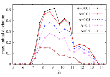
(a) (b)
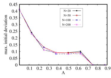
(c)

Figure 4: Stability of a 1D chain of Kapitza pendula with nearest neighbour coupling: the maximum initial deviation from the inverted position $\phi=\pi$, (a) for different values of applied amplitude for a set of coupling terms $\Lambda$. The other parameters are $g_{0}=1.0,\omega=5,N=100$. (b) for variation of the applied frequency for a set of the parameter $\Lambda$. The other parameters are $g_{0}=1.0,g_{1}=10,N=100$. (c) for variation of $\Lambda$ for different sizes of the system. The other parameters are $g_{0}=1.0,g_{1}=10,\omega=5$.

We consider a system of $N$ coupled identical Kapitza pendula, $N$ being large. Following Ref. Citro2015 the system can be cast into the following Hamiltonian

$$H=\sum_{i,j=i\pm 1}\Lambda\Big{(}\frac{p_{i}^{2}}{2}-\cos(\phi_{i}-\phi_{j})\Big{)}-\sum_{i}\frac{g(t)}{\Lambda}\cos{\phi_{i}}.$$ (2)

The energy scale $\Lambda$ determines the relative importance of the coupling between the pendula and the potential energy of individual pendulum. The coupling is restricted to the nearest neighbours only. We assume periodic boundary condition. The system equations are

$$\dot{\phi_{i}} =\Lambda p_{i},$$ (3a)

$$\dot{p_{i}} =-\Big{(}\frac{g(t)}{\Lambda}\sin{\phi_{i}}+\Lambda\sin(\phi_{i}-\phi_{j})\Big{)}.$$ (3b)

Figure 5: (Color online) Time series for nn coupling for different values of $\Lambda=0.001$ (upper panel). We observe only oscillation of $\phi$ around the inverted position. For $\Lambda=0.5$, all pendula start to rotate i.e., stability is completely lost(lower panel). Plots are shown after the transients die down (here, we show time-series for $t=1800$ to $t=2000$).

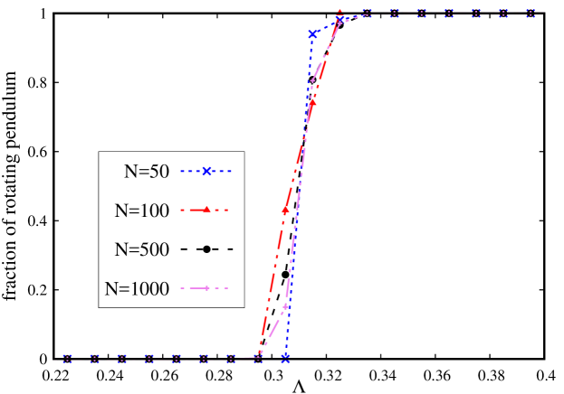
Figure 6: (Color online) Fraction of rotating pendula for nearest neighbour coupling for different system sizes. For small values of $\Lambda$ each pendulum shows oscillation around the inverted position, For a very small range of $\Lambda$ the system shows both oscillation and rotational motion. After crossing the threshold every pendulum starts to rotate.

The numerical results are presented in Fig. 4. Fig. 4(a) shows the maximum initial angle versus $g_{1}$ curves. As we increase the value of $\Lambda$ the height of the curve decreases implying decrement of stability range. As the interaction between the nearest neighbours increases gradually, stabilization is disturbed. In the simulation, each pendulum is started from slightly different initial conditions. The initial angular position($\phi$) of each pendulum is taken to be $\pi+0.001$ with some random deviation($\mathcal{O}(10^{-3})$) for each pendulum.

Fig. 4(b) shows the curves for maximum initial angle versus the driving frequency. It exhibits a similar nature of the shape of the curves. It shows that the system is stable only over a range of $\omega\sim[4,7]$ and that the stability margin degrades with increase of the coupling strength $\Lambda$. Fig. 4(c) shows the effect of the size of the system. We have studied cases for $N=20,50,100,200,500$. It shows that the stability reduces with increase in $\Lambda$, and that this result does not significantly depend on the system size $N$.

Now we explore the coupled behaviour in the system. The time series for this system is shown in Fig.5. It shows that for low values of $\Lambda$ (e.g., $\Lambda=0.001$), each pendulum oscillates (stable mode) around the inverted position. This behavior is lost when $\Lambda$ is increased to around $0.5$. Most of the pendula lose stability (go into rotating motion). We show the fraction of pendula going into rotational motion as we increase the interaction $\Lambda$ in Fig. 6. We find that for different system size, the rotational motion starts when $\Lambda\approx 0.3$. Each point in the plot is averged value of $20$ different initial conditions for each pendulum.

3.2 Case 2: 2D square network of Kapitza pendula with nearest neighbour coupling

In order to understand the effect of dimension we investigate the case of a 2D square network with nn coupling. Following the same procedure as in the 1D case, we construct the Hamiltonian for this case which can be written as

$$H=\sum_{i,j,k,l}\Lambda\Big{(}\frac{p_{i}^{2}}{2}-\cos(\phi_{i,j}-\phi_{k,l})\Big{)}-\sum_{i,j}\frac{g(t)}{\Lambda}\cos{\phi_{i,j}},$$ (4)

where $i,j$ represent indices in $x$ and $y$ directions and $k=i\pm 1,l=j\pm 1$. Here the interaction is with the nearest neighbours only, i.e., each pendulum is connected to its four nearest neighbours.

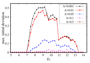
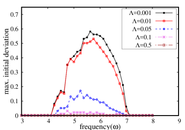
(a) (b)
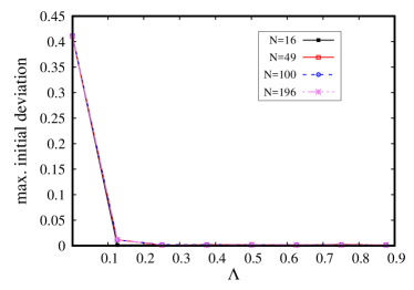
(c)

Figure 7: 2D square lattice of Kapitza pendula with nearest neighbour coupling. The maximum initial deviation from the inverted position $\phi=\pi$, (a) for different values of applied frequency for a set of the coupling term $\Lambda$. Parameters are $g_{0}=1.0$, $g_{1}=10$, $N=100$. (b) for different values of applied frequency for a set of the coupling term $\Lambda$. (c)for variation of $\Lambda$ for different sizes of the system. Parameters are $g_{0}=1.0,\omega=5,N=100$.

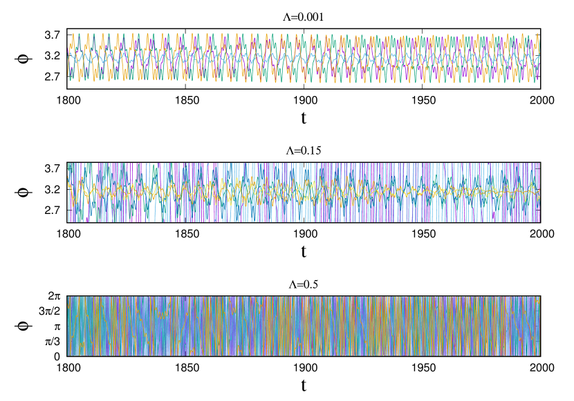
Figure 8: Figure shows time-series for three different values of $\Lambda$ for the 2D square network with nearest neighbour coupling. Parameters are $N=1000$. (a) For $\Lambda=0.001$, all pendula show oscillation arounf $\phi=\pi$. (b) For $\Lambda=0.1$, some oscillates, some rotates. Total integration time $t=2000$. We show time-series for $t=1800$ to $t=2000$ in this figure to remove transients effect.

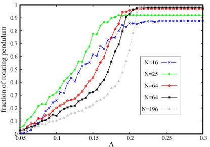
Figure 9: Fraction of rotating pendulum for 2D square network. For very small value of $\Lambda$ pendulum shows oscillation around the inverted position. As $\Lambda$ increases some fraction of pendula starts rotating motion. All pendulum starts rotating once the threshold value of $\Lambda$ is passed.

The numerical results for this system are shown in Fig.7. Fig.7(a) shows the maximum release angle versus $g_{1}$ curves. As we increase the value of $\Lambda$ the height of the curve decreases, implying decrement of stability range. However, the rate of decrement is higher compared to the 1D case. Fig. 7(b) shows the curves for maximum initial angle versus the driving frequency. Fig. 7(c) shows the effect of the size of the system. We studied the cases for $N=4\times 4,7\times 7,10\times 10,14\times 14$ square lattices. It shows that the stability reduces with increase in $\Lambda$ and the system is insensitive to the system size $N$.

Now we explore the coupled behaviour in the system. The time series is shown in Fig. 8. It shows that for small magnitude of $\Lambda$ all pendula oscillate around the inverted position. This behavior is lost when $\Lambda$ is increased. For $\Lambda=0.15$, some of the pendula oscillate, whereas, rest of them start rotating as shown in Fig.8(b). As $\Lambda$ is further increased, stability is lost and most of the pendula also go into rotating motion. In Fig. 9, we show how the fraction of total pendula exhibits oscillation and rotation for different values of $\Lambda$. For very small values, only oscillatory motion around the inverted position is observed. For higher values, all pendula start rotation. There is a range between these two kind of motion where both oscillatory and rotational motion is observed in the system. This is analogous to “chimera state”, simultaneous presence of synchronous(frequency locked) and asynchrounous (rotational motion with no synchrony among the pendula) state in the system.

3.3 Case 3 : Pendulum chain with all-to-all interaction

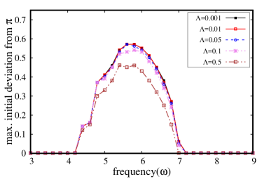
(a) (b)
(c)

Figure 10: Inverted pendula with all-to-all coupling. The maximum initial deviation from the inverted position $\phi=\pi$, (a) for different values of applied frequency for a set of coupling term $\Lambda$; the parameters are $g_{0}=1.0,g_{1}=10,N=100$, (b) for different values of applied amplitude for a set of the coupling term $\Lambda$; the parameters are $g_{0}=1.0$, $\omega=5$, $N=100$, (c) for different system sizes ($N$); the parameters are $g_{0}=1.0,\;g_{1}=10$ and $\omega=5$.

In this section we consider many body Kapitza pendulum with all to all interaction. The Hamiltonian governing the dynamics is

$$H=\sum_{i}\Big{(}\Lambda\frac{p_{i}^{2}}{2}-\frac{g(t)}{\Lambda}\cos{\phi_{i}}\Big{)}-\frac{\Lambda}{N}\sum_{i,j}\cos(\phi_{i}-\phi_{j})$$ (5)

and equations of motion are

$$\dot{\phi_{i}} =\Lambda p_{i},$$ (6a)

$$\dot{p_{i}} =-\Big{(}\frac{g(t)}{\Lambda}\sin{\phi_{i}}+\frac{\Lambda}{N}\sin(\phi_{i}-\phi_{j})\Big{)}.$$ (6b)

The interaction term is scaled by the total number of pendula $N$ to make it thermodynamically stable. Applying mean field theory we can define an order parameter for such a system with long range interaction Antoni1995 . The order parameter for the system is of the form

$$\mathbf{R}=re^{i\phi}=\frac{1}{N}\sum_{i=i}^{N}\mathbf{r}_{i}$$ (7)

where $r$ and $\phi$ represent the modulus and the phase of the order parameter and $\mathbf{r}_{i}=(\cos{\phi_{i}},\sin{\phi_{i}})$. Now the potential can be rewritten as a sum of single particle potentials

$$v_{i}=1-\Lambda M\cos(\theta_{i}-\phi).$$ (8)

Fig.10(a) shows the maximum release angle versus $g_{1}$ curves for this system. With the increase of $\Lambda$, the height of the curve decreases which implies the decrement of the stability range. Compared to the 1D and 2D case, the rate of decrement is least for this all-to-all coupling. Fig. 10(b) shows the curves for maximum initial angle versus the driving frequency. To observe the effect of system size we studied the cases for $N=20,50,100,200,500$. Fig. 10(c) shows that for a fixed value of $\Lambda$ the stability increases as we increase the size of the system.

We show the time series in Fig. 11 for $\Lambda=0.001$ and $\Lambda=0.5$. Unlike 1D and 2D case, we observe only oscillation around the inverted position in this range of $\Lambda$; we do not see any rotation in all-to-all coupling. However, in this case, beat appears in the system. At low values of $\Lambda$ clustering is not apparent. But careful examination reveals that the beats observed in the individual pendula are not the same. A few examples of different beat patterns are shown in Fig. 12. A few pendula form groups that follow the same envelop of the beat pattern.

Group	No.of pendula
1	11
2	6
3	7
4	4
5	9
6	5
7	2
8	2
not clustered	2

Table 1: Table showing clustered and unclustered pendulum for $\Lambda=0.001.$

Group	No.of pendula
1	13
2	3
3	5
4	10
5	4
6	3
7	2
8	2
9	4
not clustered	3

Table 2: Table showing clustered and unclustered pendulum for $\Lambda=0.1.$

Figure 11: Time series for all to all coupling for $\Lambda=0.001$(upper panel) and $\Lambda=0.5$ (lower panel). Parameters are : $N=1000,g_{0}=1,g_{1}=10,\omega=5$. In both cases, all pendula oscillate around $\phi=\pi$ (we have shown only $5$ pendula in this figure). Total integration time $t_{f}=2000$ and to avoid transient effect we show $t=1800$ to $t=2000$ in this figure.

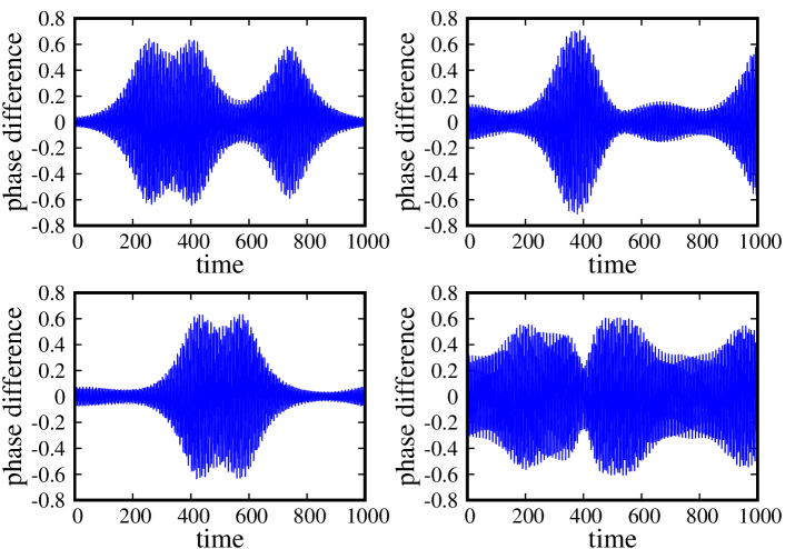
Figure 12: This figure shows the time-series of relative angular displacement $\delta\phi=\phi_{i}-\phi_{1}$, where indices $1$ and $i$ corresponds to $1\textsuperscript{st}$ and $i\textsuperscript{th}$ pendulum. This is when $\Lambda=1$. These specific envelops correspond to Group - ii@, iv@, v@ and Group -vi@ of Table. 4.

Group	No.of pendula
1	5
2	5
3	3
4	4
5	13
6	8
7	2
8	2
9	2
10	3
not clustered	2

Table 3: Table shows groups of clustered pendula. We consider $N=50,\Lambda=0.5$.

Group	No.of pendula
1	13
2	13
3	9
4	5
5	5
6	2
not clustered	2

Table 4: Table shows the number of pendula belonging to different clusters when $\Lambda=1,N=50$.

We consider $N=50$ and catagorise the pendula into group according to the envelop they belong to. List of pendula and their corresponding group is presented in Table 2, 2, 4 and 4. As soon as $\Lambda$ increases pendula start to form clusters. Some of them remain unclustered. In the clustered group, some pendula may have some phase difference. However, as we increase $\Lambda$, the phase difference vanishes and pendula are in complete synchrony with each other for a specific envelop.

Our intention was to show that clustering exists. However, which specific pendulum will belong to which cluster may vary from simulation to simulation depending on the choice of (random) initial conditions. But the number of pendula in a group remains more or less same.

4 Conclusions

In this paper we have considered systems of coupled Kapitza pendula in three different network structures. We have studied the effects of the coupling between pendula (embodied in the coupling parameter $\Lambda$ in our formulation), the network dimension ($D$), and the system size ($N$) on the stability of the system.

Increase in the coupling parameter $\Lambda$ is found to reduce the stability margins. The effect of $\Lambda$ is significant in 1D lattice but becomes very pronounced in 2D lattice with nn coupling. The effect, however, reduces for all-to-all coupling. The system size, i.e., the number of coupled pendula $N$, also plays an important role. For the all-to-all coupled system, an increase in system size drastically improves the stability of the system. But the nearest neighbour coupled lattice is relatively insensitive to the system size.

We have also explored the collective behaviour in these three networks for $\Lambda\sim[0.01,1.0]$. As we increase the value of $\Lambda$, rotational motion appears in nn coupled 1D and 2D networks. However, we do not see any such rotation in the all-to-all coupling but in this case beat appears in the system. Careful study of the beating in the all-to all case, reveals the appearance of several shapes of envelop. Once the individual time-series are catagorised into different groups corresponding to the different shapes of the envelops, clustering becomes evident.

- (1) Wolfgang Paul. Electromagnetic traps for charged and neutral particles. Rev. Mod. Phys., 62:531–540, Jul 1990.
- (2) Ido Gilary, Nimrod Moiseyev, Saar Rahav, and Shmuel Fishman. Trapping of particles by lasers: the quantum kapitza pendulum. Journal of Physics A: Mathematical and General, 36(25):L409, 2003.
- (3) Francesco Bullo. Averaging and vibrational control of mechanical systems. SIAM Journal on Control and Optimization, 41(2):542–562, 2002.
- (4) Y. Nakamura, T. Suzuki, and M. Koinuma. Nonlinear behavior and control of a nonholonomic free-joint manipulator. IEEE Transactions on Robotics and Automation, 13(6):853–862, Dec 1997.
- (5) Andrew Stephenson. XX. on induced stability. Philosophical Magazine Series 6, 15(86):233–236, 1908.
- (6) D. ter Haar (Eds.). Collected Papers of P.L. Kapitza. Volume 2. pergamon, 1st edition, 1965.
- (7) Sang-Yoon Kim and Bambi Hu. Bifurcations and transitions to chaos in an inverted pendulum. Phys. Rev. E, 58:3028–3035, Sep 1998.
- (8) Eugene I. Butikov. On the dynamic stabilization of an inverted pendulum. American Journal of Physics, 69(7):755–768, 2001.
- (9) H.W. Broer, I. Hoveijn, M. van Noort, and G. Vegter. The inverted pendulum: A singularity theory approach. Journal of Differential Equations, 157(1):120 – 149, 1999.
- (10) H. W. Broer, I. Hoveijn, M. van Noort, C. Simó, and G. Vegter. The parametrically forced pendulum: A case study in 1 1/2 degree of freedom. Journal of Dynamics and Differential Equations, 16(4):897–947, 2004.
- (11) M. V. Bartuccelli, G. Gentile, and K. V. Georgiou. On the dynamics of a vertically driven damped planar pendulum. Proceedings of the Royal Society of London A: Mathematical, Physical and Engineering Sciences, 457(2016):3007–3022, 2001.
- (12) M. V. Bartuccelli, G. Gentile, and K. V. Georgiou. On the stability of the upside–down pendulum with damping. Proceedings of the Royal Society of London A: Mathematical, Physical and Engineering Sciences, 458(2018):255–269, 2002.
- (13) Michele V Bartuccelli, Guido Gentile, and Kyriakos V Georgiou. Kam theory, lindstedt series and the stability of the upside-down pendulum. Discrete and Continuous Dynamical Systems, 9(2):413–426, 2003.
- (14) André Eckardt. Colloquium. Rev. Mod. Phys., 89:011004, Mar 2017.
- (15) R Chacon and L Marcheggiani. Controlling spatiotemporal chaos in chains of dissipative kapitza pendula. Physical Review E, 82(1):016201, 2010.
- (16) Laura Marcheggiani, Ricardo Chacón, and S Lenci. On the synchronization of chains of nonlinear pendula connected by linear springs. The European Physical Journal: Special Topics, 223(4):729–756, 2014.
- (17) Jeff Moehlis. On the dynamics of coupled parametrically forced oscillators. In Proceedings of 2008 ASME Dynamic Systems and Control Conference. Ann Arbor, Michigan, USA, 2008.
- (18) Per Danzl and Jeff Moehlis. Weakly coupled parametrically forced oscillator networks: existence, stability, and symmetry of solutions. Nonlinear Dynamics, 59(4):661–680, Mar 2010.
- (19) Y. Xu, T. J. Alexander, H. Sidhu, and P. G. Kevrekidis. Instability dynamics and breather formation in a horizontally shaken pendulum chain. Phys. Rev. E, 90:042921, Oct 2014.
- (20) P. Salgado Sánchez, J. Porter, I. Tinao, and A. Laverón-Simavilla. Dynamics of weakly coupled parametrically forced oscillators. Phys. Rev. E, 94:022216, Aug 2016.
- (21) Roberta Citro, Emanuele G Dalla Torre, Luca D’Alessio, Anatoli Polkovnikov, Mehrtash Babadi, Takashi Oka, and Eugene Demler. Dynamical stability of a many-body kapitza pendulum. Annals of Physics, 360:694–710, 2015.
- (22) André Eckardt, Christoph Weiss, and Martin Holthaus. Superfluid-insulator transition in a periodically driven optical lattice. Phys. Rev. Lett., 95:260404, Dec 2005.
- (23) H. Lignier, C. Sias, D. Ciampini, Y. Singh, A. Zenesini, O. Morsch, and E. Arimondo. Dynamical control of matter-wave tunneling in periodic potentials. Phys. Rev. Lett., 99:220403, Nov 2007.
- (24) J. Struck, C. Ölschläger, R. Le Targat, P. Soltan-Panahi, A. Eckardt, M. Lewenstein, P. Windpassinger, and K. Sengstock. Quantum simulation of frustrated classical magnetism in triangular optical lattices. Science, 333(6045):996–999, 2011.
- (25) J. Struck, C. Ölschläger, M. Weinberg, P. Hauke, J. Simonet, A. Eckardt, M. Lewenstein, K. Sengstock, and P. Windpassinger. Tunable gauge potential for neutral and spinless particles in driven optical lattices. Phys. Rev. Lett., 108:225304, May 2012.
- (26) Angelo Russomanno, Alessandro Silva, and Giuseppe E. Santoro. Periodic steady regime and interference in a periodically driven quantum system. Phys. Rev. Lett., 109:257201, Dec 2012.
- (27) Pedro Ponte, Anushya Chandran, Z. Papić, and Dmitry A. Abanin. Periodically driven ergodic and many-body localized quantum systems. Annals of Physics, 353:196 – 204, 2015.
- (28) Pedro Ponte, Z. Papić, Fran çois Huveneers, and Dmitry A. Abanin. Many-body localization in periodically driven systems. Phys. Rev. Lett., 114:140401, Apr 2015.
- (29) James A. Blackburn, H. J. T. Smith, and N. Gro/nbech‐Jensen. Stability and hopf bifurcations in an inverted pendulum. American Journal of Physics, 60(10):903–908, 1992.
- (30) Mickael Antoni and Stefano Ruffo. Clustering and relaxation in hamiltonian long-range dynamics. Phys. Rev. E, 52:2361–2374, Sep 1995.