Velocity-Space Cascade in Magnetized Plasmas: Numerical Simulations
Abstract
Plasma turbulence is studied via direct numerical simulations in a two-dimensional spatial geometry. Using a hybrid Vlasov-Maxwell model, we investigate the possibility of a velocity-space cascade. A novel theory of space plasma turbulence has been recently proposed by Servidio et al. [PRL, 119, 205101 (2017)], supported by a three-dimensional Hermite decomposition applied to spacecraft measurements, showing that velocity space fluctuations of the ion velocity distribution follow a broad-band, power-law Hermite spectrum , where is the Hermite index. We numerically explore these mechanisms in a more magnetized regime. We find that (1) the plasma reveals spectral anisotropy in velocity space, due to the presence of an external magnetic field (analogous to spatial anisotropy of fluid and plasma turbulence); (2) the distribution of energy follows the prediction , proposed in the above theoretical-observational work; and (3) the velocity-space activity is intermittent in space, being enhanced close to coherent structures such as the reconnecting current sheets produced by turbulence. These results may be relevant to the nonlinear dynamics weakly-collisional plasma in a wide variety of circumstances.
Plasma turbulence is a challenging problem, involving a variety of complex nonlinear phenomena. In the classical picture of turbulence, both in ordinary fluids and collisional plasmas, whenever energy is injected into the system, a cross-scale transfer occurs, producing smaller scales and leading eventually to energy conversion and dissipation. This non-linear behavior transfers energy from macroscopic gradients into small plasma eddies, waves and magnetic structures. The story becomes even more challenging in weakly collisional plasmas —systems far from local thermal (Maxwellian) equilibrium. The absence of an equilibrium attractor leaves the plasma state free to explore the dual spatial-velocity phase space (Huang, 1963). This dynamics is responsible for strong deformations of the particle distribution function (DF), commonly classified as rings, beams, temperature anisotropy, velocity-space vortices, and so on (Krall and Trivelpiece, 1973; Marsch et al., 1982; Hellinger et al., 2006; Burch et al., 2016). In this multi-dimensional space, energy can be transfered nonlinearly from physical space to velocity space, and vice-versa, leading finally to the dissipation of the available energy through collisions (Huang, 1963; Mikhailovskii, 1974; Pezzi, Valentini, and Veltri, 2016; Howes, 2018).
The connection between turbulence and velocity-space deformations remains a great challenge for both theoretical and computational approaches. This scenario has been envisioned since the seminal works by Landau (Landau, 1946). Recently, the study of phase-space fluctuations has become a topic of renewed interest within the plasma community (Tatsuno et al., 2009; Parker et al., 2016; TenBarge and Howes, 2013; Cerri, Kunz, and Califano, 2018). Many important and useful suggestions on the possibility of a spatial-velocity cascade have been recently proposed, in the framework of reduced models of plasma turbulence such as drift-wave and gyrokinetics (Kanekar et al., 2015; Schekochihin et al., 2016). These concepts, closely related to strongly magnetized laboratory plasmas (Eltgroth, 1974), need to be revised and further explored in the framework of space plasmas, where magnetic fluctuations are, very often, of the order of the mean magnetic field (Goldstein, Roberts, and Matthaeus, 1995). In these regimes, indeed, nonlinear Landau damping and ion-cyclotron resonances, as well as interactions with current layers and zero-frequency structures, might occur in a more complex way (Howes, Klein, and Li, 2017; Pezzi et al., 2017a).
In the last decade or so, Vlasov-based simulations have been extensively used to investigate the complexity of plasma turbulence (Howes et al., 2008; Parashar et al., 2009; Servidio et al., 2012; Wan et al., 2015; Valentini, F. et al., 2017; Pezzi et al., 2017b; Servidio et al., 2016; Franci et al., 2015a, b; Hellinger et al., 2015). Numerical experiments suggest a strong connection between turbulence and non-Maxwellian features in the particle DF Greco et al. (2012); Chasapis et al. (2017); Sorriso-Valvo et al. ; Sorriso-Valvo et al. (2018). Recently, the unprecedented-resolution and high-accuracy of measurements from the Magnetospheric Multiscale Mission (MMS) (Burch et al., 2016) have enabled direct observation of the velocity space cascade in a space plasmas (Servidio et al., 2017). In particular, a three-dimensional (3D) Hermite decomposition has been applied to spacecraft measurements, showing that the ion velocity distribution has a broad-band Hermite spectrum , where is an Hermite mode index (see below). A Kolmogorov-like phenomenology has been proposed to interpret the observations, suggesting two types of phase-space cascade: (1) the isotropic cascade, with , when the plasma is weakly magnetized (such as in the terrestrial, shocked magnetosheath), and (2) , for more highly magnetized cases. Here we inspect the latter situations, exploring the possibility of an anisotropic cascade in velocity space, establishing its relation with spatial intermittency.
In this Letter we employ Hermite decomposition to analyze a hybrid Vlasov-Maxwell (HVM) simulation Valentini et al. (2014); Servidio et al. (2015) of collisonless plasma dynamics. Noise-free HVM simulations are well-suited for the study of the kinetic effects in turbulent collisionless plasmas. We integrate the dimensionless HVM equations written as
| (1) | |||
| (2) |
where is the proton DF, and are the electric and magnetic fields, respectively. The current density is , and represent the first two moments of , and is the isothermal pressure of the massless fluid electrons. In the above equations, time, velocities and lengths are respectively scaled to the inverse proton cyclotron frequency , to the Alfvén speed , and to the proton skin depth , where , , , and the proton mass, charge, the light speed, the background magnetic field and the equilibrium proton density. A small resistivity is introduced to suppress numerical instabilities.
Equations (1)–(2) are integrated in a 2.5D–3V phase space domain. We discretized the double-periodic spatial domain of size , with grid-points in each direction. The velocity domain is discretized by points in the range and boundary conditions impose , being the proton thermal speed, related to the Alfvén speed through . Further details on the numerics can be found in Refs. Valentini et al. (2007); Perrone, Valentini, and Veltri (2011). The proton DF is initially Maxwellian, with uniform unit density. In order to explore the possibility of a magnetized phase-space cascade, a uniform background out-of-plane magnetic field () is also imposed. The equilibrium is then perturbed through a spectrum of Fourier modes, as described in Servidio et al. (2015). The r.m.s. level of fluctuations is . Note that this parameter range is very different from the MMS observations, where and (weakly magnetized regime) (Servidio et al., 2017).
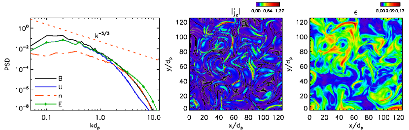
We will discuss the results at the peak of the nonlinear activity, namely at , where reaches its maximum. To characterize the presence of small-scale fluctuations, the left panel of Fig. 1 reports the omnidirectional perpendicular power spectral density of magnetic field (black), proton bulk speed (blue), electric field (green dotted) and proton density (red dashed), as a function of . The red dotted line indicates, as a reference, the Kolmogorov exponent . Magnetic fluctuations dominate at the large scales and the inertial range, while at smaller kinetic scales electric field spectral power is higher (Bale et al., 2005). Moreover, although the large scales are essentially incompressible, at kinetic scales the compressibility increases (Not, ).
Strong current sheets are evident in the shaded-contour of Fig. 1 (central panel), which shows the out-of-plane current density at . As expected in turbulence, local narrow current layers develop and become important sites of reconnection and dissipation (Servidio et al., 2015; Retinò et al., 2007; Osman et al., 2011; Karimabadi et al., 2013). Previous works have suggested that these intermittent regions are related to interesting non-Maxwellian features of the DF (Greco et al., 2012), a very well known property of magnetic reconnection (Drake et al., 2003, 2010; Swisdak, 2016). A simple non-Maxwellianity indicatorGreco et al. (2012); Pezzi et al. (2017c), measuring deviations of the particle DF from the corresponding Maxwellian , has been defined as
| (3) |
The right panel of Fig. 1 shows at , suggesting that the non-fluid activity is highly intermittent, correlated with the most intense current sheets. The scalar function quantifies the presence of high-order moments of the plasma, and includes moments of the proton DF, such as temperature anisotropy, heat flux, kurtosis and so on. It does not reveal, however, the particular structure of the velocity subspace.
In order to quantify details of the phase-space cascade, we will adopt a 3D Hermite transform representation of , a valuable tool for plasma theory (Grad, 1949; Armstrong and Montgomery, 1967; Schumer and Holloway, 1998). A 1D basis can be defined as
| (4) |
where and are now the local bulk and thermal speed, respectively, and is an integer (we simplified the notation suppressing the spatial dependence). The eigenfunctions obey the orthogonality condition . Using this basis, one obtains a 3D representation of the distribution function . The above projection quantifies high-order corrections to the particle velocity DF, since the basis is shifted in the local fluid velocity frame, normalized to the ambient density and temperature. The projection in Eq. (4) is equivalent to shifting the Hermite grid in the local plasma frame, renormalizing such that the temperature is unity. Missing the above shift would generate a convolution with the central Maxwellian kernel and therefore a misleading spectrum. Moreover, a Gaussian quadrature is adopted (Yin, 2014; Servidio et al., 2017), for efficiency, and to avoid spurious aliasing and convergence problems. We tested the accuracy of our Hermite transform, verifying that the Parseval-Plancerel spectral theorem is satisfied up to the machine precision.
Using the above procedure, the Hermite coefficients have been computed. Note that the Hermite projection has a profound meaning for gases, since the index roughly corresponds to an order of the velocity moments (Schekochihin et al., 2016): the coefficient corresponds to bulk flow fluctuations; corresponds to temperature deformations; to heat flux perturbations, and so on. Finally, it is worth noting that an highly deformed would produce plasma enstrophy (Knorr, 1977), defined as
| (5) |
where indicates the difference from the ambient Maxwellian, as in Eq. (3). It is interesting to note that the latter quantity is related to the Maxwellianity indicator , , and is essentially the free energy in gyrokinetics (Schekochihin et al., 2016).
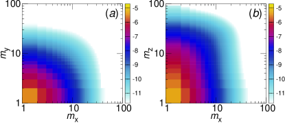
In the Hermite transform, we set modes in each velocity direction, applying the projection to a subset of the original volume. In particular, we choose equally-spaced spatial points on a grid that is coarser than the original , to reduce computational efforts (although the algorithm uses MPI parallel architecture). We have checked that statistical convergence is attained for an ensemble of 3232 proton velocity DFs (not shown). In our analysis, we ensure convergence by using an ensemble of 6464 velocity DFs. From the coefficients , we define the enstrophy spectra as , where indicates spatial average. Note that details of the phase space structure are lost when the Hermite spectrum is computed for poorly resolved data, or when the spectrum is reduced (integrated over a velocity coordinate).
The 2D enstrophy spectrum is evaluated by reducing in different directions, as for example . Figure 2 reports the 2D reduced spectra and . The enstrophy is fairly isotropic in the plane , perpendicular to the background magnetic field. On the other hand, an anisotropy is revealed when considering the direction of , namely the axis: spectra are stretched in the parallel direction. This might indicate the presence of structures along the background field and the presence of Landau resonances (Kennel and Petschek, 1966). Note also that this anisotropy was not recovered in the magnetosheath observations of MMSServidio et al. (2017), since and were much higher than in our simulation. This anisotropy is analogous to the spatial anisotropy commonly observed in plasmas, when a strong imposed field is present (Shebalin, Matthaeus, and Montgomery, 1983). The velocity space anisotropy, however, differs in that velocity gradients are stronger along the mean field and the cascade is inhibited across the mean field.
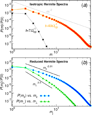
We evaluated the isotropic (omnidirectional) 1D Hermite spectra, by summing over concentric shells of unit width, i. e. . Figure 3(a) shows the isotropic Hermite spectrum at (we normalized the spectrum to the mode , which is the Maxwellian profile.) The spectrum shows a power-law behavior for the first decade, indicating the presence of phase-space cascade-like processes Sircombe, Arber, and Dendy (2006); Schekochihin et al. (2008); Tatsuno et al. (2009); Hatch et al. (2014); Kanekar et al. (2015); Parker and Dellar (2015); Parker et al. (2016); Schekochihin et al. (2016); Servidio et al. (2017). The Hermite analysis on the HVM simulations shows a spectral break around , where the artificial dissipation of the Eulerian scheme might affect the dynamics. In the same panel (a), we also plot the energy at an earlier time of the simulation, showing that the cascade has progressively emerged, as it would in physical space, by gradually filling in modes towards higher -values, therefore creating finer velocity-space structures. In Fig. (3)-(b), we show the reduced spectra along the mean field (integrated over and ), and the isotropic perpendicular spectrum (integrated over and over concentric perpendicular shells ). While is consistent with the phenomenological model, the reduced perpendicular spectrum is much lower in energy and is steeper, with exponent close to . The significance of such anisotropy of the Hermite spectra will be investigated more in detail in future works.
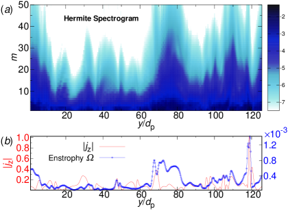
In analogy with intermittency in turbulence, it is natural to ask whether or not the enstrophy transfer is homogeneous in space, as suggested by Fig. 1 (center and right panels). To this aim, we define the Hermite spectrogram , the isotropic Hermite spectrum as a function of the position. This tool might be also useful for spacecraft measurements. Fig. 4-(a) shows along a one-dimensional spatial cut. The dual-space cascade is clearly intermittent: the spectrum amplitude and exponent depend on the position, with regions of low activity being interrupted by bursts of velocity-space activity. Only the ensemble average converges to the theoretical predictions represented in Fig. 3. In panel (b), we show a spatial cut of the current density (red) and of the plasma enstrophy (blue), suggesting that the velocity space cascade is correlated with the intermittent current structures.
Motivated by recent theories and observations(Servidio et al., 2017; Adkins and Schekochihin, 2018), we have studied plasma turbulence via direct numerical simulations, in a simplified 2.5D-3V geometry. Using a hybrid Vlasov-Maxwell model, we observed that the proton velocity distribution function produces broad-band fluctuations in the –space. By using a 3D Hermite decomposition, we observed power-law Hermite spectra , indicative of a velocity inertial range. This velocity cascade establishes as the turbulence develops, resembling a mode-by-mode transfer, similar to the Kolmogorov phenomenology. Exploring a moderately magnetized case ( and ) we found that: (1) plasma manifests spectral anisotropy in velocity space, due to the presence of an external magnetic field (analogous to the Shebalin effect (Shebalin, Matthaeus, and Montgomery, 1983)); (2) the distribution of energy follows the prediction , and a much steeper exponent in the perpendicular direction, where . Finally, (3) the velocity space activity is intermittent in real space, and is enhanced close to coherent structures such as the reconnecting current layers produced by turbulence. In future works, we plan to explore different plasma regimes, as well as the role played by the dimensionality of the system and by the electron kinetics. These results may be of fundamental significance as the space and astrophysical plasma communities move towards more complete understanding of the mechanisms leading to dissipation and heating in turbulent plasmas.
Acknowledgements.
This research was partially supported by AGS-1460130 (SHINE), NASA grants NNX14AI63G (Heliophysics Grand Challenge Theory), NNX15AB88G, NNX17AB79G, the Solar Probe Plus science team (ISOIS/Princeton subcontract SUB0000165), and by the MMS Theory and Modeling team, NNX14AC39G. FV and OP are supported by Agenzia Spaziale Italiana under contract ASI-INAF 2015-039-R.O. DP, SS ans LSV acknowledge support from the Faculty of the European Space Astronomy Centre (ESAC). Computational support is provided by the Newton cluster at UNICAL. This work is partly supported by the International Space Science Institute (ISSI) in the framework of International Team 405 entitled “Current Sheets, Turbulence, Structures and Particle Acceleration in the Heliosphere”.References
- Huang (1963) K. Huang, Statistical Mechanics, New York: Wiley, 1963 ( , 1963).
- Krall and Trivelpiece (1973) N. A. Krall and A. W. Trivelpiece, Palaeogeography Palaeoclimatology Palaeoecology (1973).
- Marsch et al. (1982) E. Marsch, K.-H. Mühlhäuser, R. Schwenn, H. Rosenbauer, W. Pilipp, and F. Neubauer, Journal of Geophysical Research: Space Physics (1978–2012) 87, 52 (1982).
- Hellinger et al. (2006) P. Hellinger, P. Trávníček, J. C. Kasper, and A. J. Lazarus, Geophys. Res. Lett. 33, L09101 (2006).
- Burch et al. (2016) J. L. Burch, T. E. Moore, R. B. Torbert, and B. L. Giles, Space Sci. Rev. 199, 5 (2016).
- Mikhailovskii (1974) A. B. Mikhailovskii, Theory of plasma instabilities. In: Instabilities in an Inhomogeneous Plasma, Vol. 2 (New York: Plenum, 1974).
- Pezzi, Valentini, and Veltri (2016) O. Pezzi, F. Valentini, and P. Veltri, Physical Review Letters 116, 145001 (2016).
- Howes (2018) G. G. Howes, ArXiv e-prints (2018), arXiv:1802.04154 [physics.space-ph] .
- Landau (1946) L. Landau, Zh. Eksp. Teor. Fiz. 16, 574 (1946).
- Tatsuno et al. (2009) T. Tatsuno, W. Dorland, A. A. Schekochihin, G. G. Plunk, M. Barnes, S. C. Cowley, and G. G. Howes, Physical Review Letters 103, 015003 (2009), arXiv:0811.2538 [physics.plasm-ph] .
- Parker et al. (2016) J. T. Parker, E. G. Highcock, A. A. Schekochihin, and P. J. Dellar, Physics of Plasmas 23, 070703 (2016), https://doi.org/10.1063/1.4958954 .
- TenBarge and Howes (2013) J. M. TenBarge and G. G. Howes, The Astrophys. J. Lett. 771, L27 (2013), arXiv:1304.2958 [physics.plasm-ph] .
- Cerri, Kunz, and Califano (2018) S. S. Cerri, M. W. Kunz, and F. Califano, ArXiv e-prints (2018), arXiv:1802.06133 [physics.plasm-ph] .
- Kanekar et al. (2015) A. Kanekar, A. A. Schekochihin, W. Dorland, and N. F. Loureiro, Journal of Plasma Physics 81, 305810104 (2015), arXiv:1403.6257 [physics.plasm-ph] .
- Schekochihin et al. (2016) A. A. Schekochihin, J. T. Parker, E. G. Highcock, P. J. Dellar, W. Dorland, and G. W. Hammett, Journal of Plasma Physics 82, 905820212 (2016), arXiv:1508.05988 [physics.plasm-ph] .
- Eltgroth (1974) P. G. Eltgroth, Physics of Fluids 17, 1602 (1974).
- Goldstein, Roberts, and Matthaeus (1995) M. L. Goldstein, D. A. Roberts, and W. H. Matthaeus, Ann. Rev. Astron. Astrophys. 33, 283 (1995).
- Howes, Klein, and Li (2017) G. G. Howes, K. G. Klein, and T. C. Li, Journal of Plasma Physics 83, 705830102 (2017).
- Pezzi et al. (2017a) O. Pezzi, F. Malara, S. Servidio, F. Valentini, T. N. Parashar, W. H. Matthaeus, and P. Veltri, Phys. Rev. E 96, 023201 (2017a).
- Howes et al. (2008) G. G. Howes, S. C. Cowley, W. Dorland, G. W. Hammett, E. Quataert, and A. A. Schekochihin, J. Geophys. Res. 113, A05103 (2008), 10.1029/2007JA012665.
- Parashar et al. (2009) T. N. Parashar, M. A. Shay, P. A. Cassak, and W. H. Matthaeus, Physics of Plasmas 16, 032310 (2009).
- Servidio et al. (2012) S. Servidio, F. Valentini, F. Califano, and P. Veltri, Physical review letters 108, 045001 (2012).
- Wan et al. (2015) M. Wan, W. H. Matthaeus, V. Roytershteyn, H. Karimabadi, T. Parashar, P. Wu, and M. Shay, Physical Review Letters 114, 175002 (2015).
- Valentini, F. et al. (2017) Valentini, F., Vásconez, C. L., Pezzi, O., Servidio, S., Malara, F., and Pucci, F., ”Astronomy and Astrophysics” 599, ”A8” (2017).
- Pezzi et al. (2017b) O. Pezzi, T. N. Parashar, S. Servidio, F. Valentini, C. L. Vásconez, Y. Yang, F. Malara, W. H. Matthaeus, and P. Veltri, The Astrophysical Journal 834, 166 (2017b).
- Servidio et al. (2016) S. Servidio, C. T. Haynes, W. H. Matthaeus, D. Burgess, V. Carbone, and P. Veltri, Physical Review Letters 117, 095101 (2016), arXiv:1608.01207 [physics.plasm-ph] .
- Franci et al. (2015a) L. Franci, S. Landi, L. Matteini, A. Verdini, and P. Hellinger, The Astrophysical Journal 812, 21 (2015a), arXiv:1506.05999 [astro-ph.SR] .
- Franci et al. (2015b) L. Franci, A. Verdini, L. Matteini, S. Landi, and P. Hellinger, The Astrophys. J. Lett. 804, L39 (2015b), arXiv:1503.05457 [astro-ph.SR] .
- Hellinger et al. (2015) P. Hellinger, L. Matteini, S. Landi, A. Verdini, L. Franci, and P. Trávníček, The Astrophysical Journal Letters 811, L32 (2015), arXiv:1508.03159 [physics.space-ph] .
- Greco et al. (2012) A. Greco, F. Valentini, S. Servidio, and W. Matthaeus, Physical Review E 86, 066405 (2012).
- Chasapis et al. (2017) A. Chasapis, W. H. Matthaeus, T. N. Parashar, O. LeContel, A. Retinò, H. Breuillard, Y. Khotyaintsev, A. Vaivads, B. Lavraud, E. Eriksson, T. E. Moore, J. L. Burch, R. B. Torbert, P.-A. Lindqvist, R. E. Ergun, G. Marklund, K. A. Goodrich, F. D. Wilder, M. Chutter, J. Needell, D. Rau, I. Dors, C. T. Russell, G. Le, W. Magnes, R. J. Strangeway, K. R. Bromund, H. K. Leinweber, F. Plaschke, D. Fischer, B. J. Anderson, C. J. Pollock, B. L. Giles, W. R. Paterson, J. Dorelli, D. J. Gershman, L. Avanov, and Y. Saito, The Astrophysical Journal 836, 247 (2017).
- (32) L. Sorriso-Valvo, D. Perrone, O. Pezzi, F. Valentini, S. Servidio, Y. Zouganelis, and P. Veltri, Journal of Plasma Physics .
- Sorriso-Valvo et al. (2018) L. Sorriso-Valvo, F. Carbone, S. Perri, A. Greco, R. Marino, and R. Bruno, Solar Physics 293, 10 (2018).
- Servidio et al. (2017) S. Servidio, A. Chasapis, W. H. Matthaeus, D. Perrone, F. Valentini, T. N. Parashar, P. Veltri, D. Gershman, C. T. Russell, B. Giles, S. A. Fuselier, T. D. Phan, and J. Burch, Phys. Rev. Lett. 119, 205101 (2017).
- Valentini et al. (2014) F. Valentini, S. Servidio, D. Perrone, F. Califano, W. Matthaeus, and P. Veltri, Physics of Plasmas 21, 082307 (2014).
- Servidio et al. (2015) S. Servidio, F. Valentini, D. Perrone, A. Greco, F. Califano, W. H. Matthaeus, and P. Veltri, Journal of Plasma Physics 81, 325810107 (2015).
- Valentini et al. (2007) F. Valentini, P. Trávníček, F. Califano, P. Hellinger, and A. Mangeney, Journal of Computational Physics 225, 753 (2007).
- Perrone, Valentini, and Veltri (2011) D. Perrone, F. Valentini, and P. Veltri, The Astrophysical Journal 741, 43 (2011).
- Bale et al. (2005) S. D. Bale, P. J. Kellogg, F. S. Mozer, T. S. Horbury, and H. Reme, Physical Review Letters 94, 215002 (2005).
- (40) Note that, with the present model and setup, we describe only the inertial range of turbulence and the proton-transition scales. The investigation of sub-proton and electron scale turbulence would require a full Vlasov description .
- Retinò et al. (2007) A. Retinò, D. Sundkvist, A. Vaivads, F. Mozer, M. André, and C. J. Owen, Nature Physics 3, 236 (2007).
- Osman et al. (2011) K. T. Osman, W. H. Matthaeus, A. Greco, and S. Servidio, Astrophys. J. Lett. 727, L11 (2011).
- Karimabadi et al. (2013) H. Karimabadi, V. Roytershteyn, M. Wan, W. H. Matthaeus, W. Daughton, P. Wu, M. Shay, B. Loring, J. Borovsky, E. Leonardis, S. C. Chapman, and T. K. M. Nakamura, Physics of Plasmas 20, 012303 (2013).
- Drake et al. (2003) F. M. Drake, M. Swisdak, C. Cattell, M. A. Shay, B. N. Rogers, and A. Zeile, Science 7, 843 (2003).
- Drake et al. (2010) J. F. Drake, M. Opher, M. Swisdak, and J. N. Chamoun, The Astrophysical Journal 709, 963 (2010), arXiv:0911.3098 [astro-ph.SR] .
- Swisdak (2016) M. Swisdak, Geophysical Research Letters 43, 43 (2016).
- Pezzi et al. (2017c) O. Pezzi, T. N. Parashar, S. Servidio, F. Valentini, C. L. Vásconez, Y. Yang, F. Malara, W. H. Matthaeus, and P. Veltri, Journal of Plasma Physics 83, 705830108 (2017c).
- Grad (1949) H. Grad, Commun. Pure Appl. Math. 2, 331 (1949).
- Armstrong and Montgomery (1967) T. Armstrong and D. Montgomery, Journal of Plasma Physics 1, 425 (1967).
- Schumer and Holloway (1998) J. W. Schumer and J. P. Holloway, Journal of Computational Physics 144, 626 (1998).
- Yin (2014) Z. Yin, Journal of Computational Physics 258, 371 (2014).
- Knorr (1977) G. Knorr, Plasma Physics 19, 529 (1977).
- Kennel and Petschek (1966) C. F. Kennel and H. Petschek, Journal of Geophysical Research 71, 1 (1966).
- Shebalin, Matthaeus, and Montgomery (1983) J. V. Shebalin, W. H. Matthaeus, and D. Montgomery, J. Plasma Phys. 29, 525 (1983).
- Sircombe, Arber, and Dendy (2006) N. J. Sircombe, T. D. Arber, and R. O. Dendy, Journal de Physique IV 133, 277 (2006).
- Schekochihin et al. (2008) A. A. Schekochihin, S. C. Cowley, W. Dorland, G. W. Hammett, G. G. Howes, G. G. Plunk, E. Quataert, and T. Tatsuno, Plasma Physics and Controlled Fusion 50, 124024 (2008), arXiv:0806.1069 [physics.plasm-ph] .
- Hatch et al. (2014) D. R. Hatch, F. Jenko, V. Bratanov, and A. B. Navarro, Journal of Plasma Physics 80, 531–551 (2014).
- Parker and Dellar (2015) J. T. Parker and P. J. Dellar, Journal of Plasma Physics 81, 305810203 (2015), arXiv:1407.1932 [physics.plasm-ph] .
- Adkins and Schekochihin (2018) T. Adkins and A. A. Schekochihin, Journal of Plasma Physics 84, 905840107 (2018).