A Family of ESDIRK Integration Methods

Abstract

In this paper we derive and analyze the properties of explicit singly diagonal implicit Runge-Kutta (ESDIRK) integration methods. We discuss the principles for construction of Runge-Kutta methods with embedded methods of different order for error estimation and continuous extensions for discrete event location. These principles are used to derive a family of ESDIRK integration methods with error estimators and continuous-extensions. The orders of the advancing method (and error estimator) are 1(2), 2(3) and 3(4), respectively. These methods are suitable for obtaining low to medium accuracy solutions of systems of ordinary differential equations as well as index-1 differential algebraic equations. The continuous extensions facilitates solution of hybrid systems with discrete-events. Other ESDIRK methods due to Kværnø are equipped with continuous-extensions as well to make them applicable to hybrid systems with discrete events.

1 Introduction

In this paper, we derive and analyze a family of explicit singly diagonally implicit Runge-Kutta (ESDIRK) integration methods which can be applied for solution of stiff systems of ordinary differential equations

(1) $$\dot{x}(t)=f(t,x(t))\qquad x(t_{0})=x_{0}$$

as well as index-1 semi-explicit systems of differential algebraic equations

(2a) $$\dot{x}(t) =f(t,x(t),y(t))\qquad x(t_{0})=x_{0}$$

(2b) $$0 =g(t,x(t),y(t))$$

in which $t\geq t_{0}\subset\mathbb{R}$, $x\in\mathbb{R}^{n}$, and $y\in\mathbb{R}^{m}$. For notational simplicity, we discuss the ESDIRK method for (1), but constructed with properties such that it is equally applicable to (2). A common notation for (1) and (2) is

(3) $$M\dot{x}(t)=f(t,x(t))\qquad x(t_{0})=x_{0}$$

in which the matrix $M$ may be singular. In addition it may depend of $t$ and $x(t)$, i.e. $M=M(t,x(t))$.

Numerical methods for solution of these systems are not only of importance in simulation, but are finding an increasing number of applications in numerical tasks related to nonlinear predictive control [3, 9]. These tasks include experimental design, parameter and state estimation, and numerical solution of optimal control problems. While linear multistep methods such as BDF based implementations, e.g. DASPK [20, 44, 35], DAEPACK [41, 19, 47, 48, 5], and DAESOL [8, 7, 6] have been applied successfully to such problems, it has been observed that typical industrial problems related to nonlinear predictive control applications have frequent discontinuities. Therefore, one-step methods, e.g. SLIMEX [43] and ESDIRK [32], are more efficient for the solution of such problems than linear multi-step BDF methods.

Singly diagonally implicit Runge-Kutta methods (SDIRK) are incepted by Butcher [11] and have been applied for solving systems of stiff ordinary differential equations since their general introduction in the 1970s [36, 1]. They have been provided in implementations such as DIRKA and DIRKS [17, 18], SIMPLE [39, 37, 38], and SDIRK4 [24]. SDIRK methods with an explicit first stage equal to the last stage in the previous step are called ESDIRK methods. They are of a much more recent origin and was first considered as a general integration method for systems of stiff systems in the years around year 2000 [15, 16, 13, 50, 49, 2, 34]. They retain the excellent stability properties of implicit Runge-Kutta methods and compared to SDIRK methods improve the computational efficiency. ESDIRK methods have been applied in implicit-explicit Runge-Kutta methods for solution of convection-diffusion-reaction problems [4, 40, 29, 30], in dynamic optimization and optimal control applications for efficient sensitivity computation [32, 31, 33], and for very computationally efficient implementations of extended Kalman filters [27, 28].

In this paper, we derive and present a family of ESDIRK methods suitable for numerical integration of stiff systems of differential equations (1) as well as index-1 differential algebraic systems (2). The methods are characterized in terms of A- and L-stability as well as order of the basic integrator and the embedded method for error estimation. We equip the methods with continuous-extensions such that they can be applied to discrete-event systems. The paper is organized as follows. In Section 2, we present and discuss Runge-Kutta methods and the general principles for their implementation and construction. Section 3 applies these principles for construction of ESDIRK methods while we discuss other ESDIRK methods in Sections 4 and 5. The other ESDIRK methods are equipped with continuous extensions. Concluding remarks and a summarily comparison of the ESDIRK methods are given in Section 6. A companion paper discusses implementation aspects and computational properties of the ESDIRK algorithms [26].

2 Runge-Kutta Integration Methods

The numerical solution of systems of differential equations (1) by an s-stage Runge-Kutta method, may in each integration step be denoted

(4a) $$T_{i} =t_{n}+c_{i}h\qquad i=1,2,\ldots,s$$

(4b) $$X_{i} =x_{n}+h\sum_{j=1}^{s}a_{ij}f(T_{j},X_{j})\qquad i=1,2,\ldots,s$$

(4c) $$x_{n+1} =x_{n}+h\sum_{j=1}^{s}b_{j}f(T_{j},X_{j})$$

(4d) $$\hat{x}_{n+1} =x_{n}+h\sum_{j=1}^{s}\hat{b}_{j}f(T_{j},X_{j})$$

(4e) $$e_{n+1} =x_{n+1}-\hat{x}_{n+1}=h\sum_{j=1}^{s}d_{j}f(T_{j},X_{j})\quad d_{j}=b_{j}-\hat{b}_{j}$$

$T_{i}$ and $X_{i}$ are the internal nodes and states computed by the s-stage Runge-Kutta method. $x_{n+1}$ is the state computed at $t_{n+1}=t_{n}+h$. $\hat{x}_{n+1}$ is the corresponding state computed by the embedded Runge-Kutta method and $e_{n+1}=x_{n+1}-\hat{x}_{n+1}$ is the estimated error of the numerical solution, i.e. $\left\|e_{n+1}\right\|$ is an estimate of the local error, $\left\|x_{n+1}-x(t_{n+1})\right\|$ given $x(t_{n})=x_{n}$. The embedded method, $\hat{x}_{n+1}$, uses the same internal stages as the integration method, but the quadrature weights are selected such that the embedded method is of different order, which then provides an error estimate for the lowest order method. This order relation of the integration method and the embedded method is utilized by the error controller to adjust the step size, $h$, adaptively [21, 22, 45, 46].

Alternatively, the s-stage Runge-Kutta method may be denoted and implemented according to

(5a) $$T_{i} =t_{n}+c_{i}h\qquad i=1,2,\ldots,s$$

(5b) $$X_{i} =x_{n}+h\sum_{j=1}^{s}a_{ij}\dot{X}_{j}\qquad i=1,2,\ldots,s$$

(5c) $$\dot{X}_{i} =f(T_{i},X_{i})=f(T_{i},x_{n}+h\sum_{j=1}^{s}a_{ij}\dot{X}_{j})\qquad i=1,2,\ldots,s$$

(5d) $$x_{n+1} =x_{n}+h\sum_{j=1}^{s}b_{j}\dot{X}_{j}$$

(5e) $$\hat{x}_{n+1} =x_{n}+h\sum_{j=1}^{s}\hat{b}_{j}\dot{X}_{j}$$

(5f) $$e_{n+1} =x_{n+1}-\hat{x}_{n+1}=h\sum_{j=1}^{s}d_{j}\dot{X}_{j}\quad d_{j}=b_{j}-\hat{b}_{j}$$

Sometimes the notation $K_{i}=\dot{X}_{i}$ is used for this implementation. In (4) the stage values, $X_{i}$, are computed iteratively by solution of (4b), while in (5) the time derivatives of the stage values, $\dot{X}_{i}$, are computed iteratively by solution of (5c). Formally, (4) and (5) are equivalent. However, (5) is directly applicable to index-1 DAEs (2) as well as implicit DAE systems making this implementation preferred over (4).

The s-stage Runge-Kutta method with an embedded error estimator, (4) or (5), may be denoted in terms of its Butcher tableau

$$\begin{array}[]{l|l}c&A\\ \hline\cr&b^{\prime}\\ &\hat{b}^{\prime}\\ \hline\cr&d^{\prime}\end{array}\qquad=\qquad\begin{array}[]{l|llll}c_{1}&a_{11}&a_{12}&\ldots&a_{1s}\\ c_{2}&a_{21}&a_{22}&\ldots&a_{2s}\\ \vdots&\vdots&\vdots&&\vdots\\ c_{s}&a_{s1}&a_{s2}&\ldots&a_{ss}\\ \hline\cr&b_{1}&b_{2}&\ldots&b_{s}\\ &\hat{b}_{1}&\hat{b}_{2}&\ldots&\hat{b}_{s}\\ \hline\cr&d_{1}&d_{2}&\ldots&d_{s}\end{array}$$

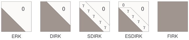
Fig. 1: Structure of the $A$-matrix for different classes of Runge-Kutta methods.

Different classes of Runge-Kutta methods may be characterized in terms of the A-matrix in their Butcher tableau. This is illustrated in Figure 1. Explicit Runge-Kutta (ERK) methods have a strictly lower triangular A-matrix implying that (5) may be solved explicitly and without iterations. Therefore, ERK methods have low computational cost but may suffer from stability limitations when applied to stiff problems. ERK methods should therefore be applied for non-stiff ODE problems, but not for stiff ODE problems (1) or DAE problems (2). All implicit Runge-Kutta methods are characterized by an A-matrix that is not lower triangular. This implies that some iterative method is needed for solution of (5). Fully implicit Runge-Kutta (FIRK) methods are characterized by excellent stability properties making them useful for solution of stiff systems of ordinary differential equations (1), systems of index-1 semi-explicit differential algebraic equations (2), as well as systems of general differential algebraic equations. However, in each integration step a system of $n\times s$ coupled nonlinear equations must be solved. The price of the excellent stability properties is high computational cost. To achieve some of the stability properties of FIRK methods but at lower computational cost, diagonally implicit Runge-Kutta (DIRK), singly diagonally implicit Runge-Kutta (SDIRK), and explicit singly diagonally implicit Runge-Kutta (ESDIRK) methods have been constructed. For the DIRK methods, the internal stages decouples in a such a way that the iterations may be conducted sequentially. This implies that in DIRK-methods, $s$ systems of $n$ nonlinear equations are solved instead of one system of $s\times n$ nonlinear equations as in the FIRK method. In the SDIRK methods, the diagonal elements are identical such that the iteration matrix may be reused for each stage. This saves a significant number of LU-factorizations in the Newton iterations. In the ESDIRK method, the first step is explicit ($c_{1}=0$ and $a_{11}=0$), the internal stages $2,\ldots,s$ are singly diagonally implicit, and the last stage is equal to the next first stage ($c_{s}=1$). This implies that the first stage is free and that the iteration matrix in stage $2,\ldots,s$ can be reused. Practical experience with ESDIRK methods shows that they retain the stability properties of FIRK methods but at significant lower computational costs.

In addition, ESDIRK methods are often constructed such that they are stiffly accurate, i.e. $a_{si}=b_{i}$ for $i=1,2,\ldots,s$ (note $b_{s}=a_{ss}=\gamma$). This implies that the last stage is equal to the final solution, $x_{n+1}=X_{s}$, and that no extra computations are needed for solution of the algebraic variables in (2). Furthermore, stiffly accurate methods avoid the order reduction for stiff systems [42]. Stiffly accurate ESDIRK methods with different number of stages and order can be represented by the following Butcher tableaus

$$\begin{array}[]{l|ll}0&0&\\ 1&b_{1}&\gamma\\ \hline\cr&b_{1}&\gamma\\ &\hat{b}_{1}&\hat{b}_{2}\\ \hline\cr&d_{1}&d_{2}\end{array}\qquad\quad\begin{array}[]{l|lll}0&0&&\\ c_{2}&a_{21}&\gamma&\\ 1&b_{1}&b_{2}&\gamma\\ \hline\cr&b_{1}&b_{2}&\gamma\\ &\hat{b}_{1}&\hat{b}_{2}&\hat{b}_{3}\\ \hline\cr&d_{1}&d_{2}&d_{3}\end{array}\qquad\quad\begin{array}[]{l|llll}0&0&&&\\ c_{2}&a_{21}&\gamma&&\\ c_{3}&a_{31}&a_{32}&\gamma&\\ 1&b_{1}&b_{2}&b_{3}&\gamma\\ \hline\cr&b_{1}&b_{2}&b_{3}&\gamma\\ &\hat{b}_{1}&\hat{b}_{2}&\hat{b}_{3}&\hat{b}_{4}\\ \hline\cr&d_{1}&d_{2}&d_{3}&d_{4}\end{array}$$

As is evident from the above Butcher tableaus, stiffly accurate ESDIRK methods with $s$ stages need only to compute $s-1$ stages as the first stage is equal to the last stage of the previous step.

2.1 Order Conditions for Runge-Kutta Methods

The order conditions for Runge-Kutta methods are developed considering Taylor expansions of the analytical and numerical solution of the autonomous ODE

(6) $$\dot{x}(t)=f(x(t))\qquad x(t_{0})=x_{0}$$

The forced ODE (1) can always be transformed into an autonomous system of ODEs (6) using

$$z(t)=\begin{bmatrix}x(t)\\ t\end{bmatrix}\quad\dot{z}(t)=\begin{bmatrix}\dot{x}(t)\\ \dot{t}\end{bmatrix}=\begin{bmatrix}f(t,x(t))\\ 1\end{bmatrix}=F(z(t))\quad z(t_{0})=\begin{bmatrix}x(t_{0})\\ t_{0}\end{bmatrix}=\begin{bmatrix}x_{0}\\ t_{0}\end{bmatrix}=z_{0}$$

Runge-Kutta methods must satisfy the consistency condition (9a) to integrate the time component correctly, i.e. to have exact equivalence between the forced system (1) and the autonomous system (6). The order conditions are usually derived considering a scalar autonomous system. This is simpler and loses no generality compared to the vector case. Let $\mathcal{T}$ denote all rooted trees and let $\mathcal{T}(p)$ denote the set of rooted trees with order less or equal to $p$, i.e. $\mathcal{T}(p)=\left\{\tau\in\mathcal{T}:\,r(\tau)\leq p\right\}$. Some functions on rooted trees are listed in Table 1. We call these trees for Butcher trees since they were first used by Butcher to derive order conditions for Runge-Kutta methods [10, 14, 12]. The advantage of Butcher trees is that the order conditions can be derived from these trees and it is significantly easier to write up all Butcher trees to a given order than ab initio derivation of the order conditions from Taylor expansions. The number of nodes (dots) in the tree corresponds to the order, $r(\tau)$, and the symmetry, $\sigma(\tau)$, is easily inspected for a tree by labelling the nodes. The density, $\gamma(\tau)$, is computed by multiplying the orders of each subtree rooted on a vertex of $\tau$, e.g. $\gamma(\tau_{7})=4\cdot 3\cdot(1\cdot 1)=12$. The matrices, $\Lambda(\tau)$, can also be derived by inspection of the Butcher trees. $\Lambda(\tau)$ is constructed as follows: a vertex connecting to a node with no further subtrees corresponds to multiplying by $C$, while a vertex connecting to a node with further subtrees corresponds to multiplying by $A$. As an example consider the tree $\tau_{6}$. The first vertex going to the left ends on a terminal node and therefore corresponds to multiplying by $C$. The first vertex going to the right does not end on a terminal node and corresponds to multiplying by $A$, while the next vertex on this branch of the tree ends on a terminal node and corresponds to multiplying with $C$. Hence, $\Lambda(\tau_{6})=CAC$. $\Phi(\tau)$ and $\Psi(\tau)$ are defined as $\Phi(\tau)=b^{\prime}\Lambda(\tau)e$ and $\Psi(\tau)=\Lambda(\tau)e$. The elementary weights $F(\tau)$ are also easily derived from the rooted tree (see Table 1).

Table 1: Some functions on rooted trees [14, 12]. $\tau$ denotes the rooted tree, $r(\tau)$ the order, $\sigma(\tau)$ the number of symmetries, and $\gamma(\tau)$ the density computed by multiplying the orders of each subtree rooted on a vertex of $\tau$. $\Lambda(\tau)$ are elementary weights derived under the consistency assumption $Ae=Ce$. $\Phi(\tau)$ and $\Psi(\tau)$ are defined by $\Phi(\tau)=b^{\prime}\Lambda(\tau)e$ and $\Psi(\tau)=\Lambda(\tau)e$. $F(\tau)$ denotes an elementary weight of $\tau$, e.g. of its use: $F(\tau_{3})(x(t_{n}))=f^{\prime\prime}(f,f)(x(t_{n}))=f^{\prime\prime}(x(t_{n}))f(x(t_{n}))f(x(t_{n}))$.

$\tau$	$\tau_{1}$	$\tau_{2}$	$\tau_{3}$	$\tau_{4}$	$\tau_{5}$	$\tau_{6}$	$\tau_{7}$	$\tau_{8}$
	\begin{picture}(1.5,3.0)(-1.0,0.0) { } {\put(0.0,0.0){}}\end{picture}	\begin{picture}(1.5,3.0)(-1.0,0.0) { } { } {\put(0.0,0.0){ }}{\put(0.0,0.0){}}{\put(0.0,1.0){}}\end{picture}	\begin{picture}(1.5,3.0)(-1.0,0.0) { } { } { } {\put(0.0,0.0){ }} {\put(0.0,0.0){ }}{\put(0.0,0.0){}}{\put(-0.5,1.0){}}{\put(0.5,1.0){}}\end{picture}	\begin{picture}(1.5,3.0)(-1.0,0.0) { } { } { } {\put(0.0,0.0){ }} {\put(0.0,1.0){ }}{\put(0.0,0.0){}}{\put(0.0,1.0){}}{\put(0.0,2.0){}}\end{picture}	\begin{picture}(1.5,3.0)(-1.0,0.0) { } { } { } { } {\put(0.0,0.0){ }} {\put(0.0,0.0){ }} {\put(0.0,0.0){ }}{\put(0.0,0.0){}}{\put(-0.75,1.0){}}{\put(0.75,1.0){}}{\put(0.0,1.0){}}\end{picture}	\begin{picture}(1.5,3.0)(-1.0,0.0) { } { } { } { } {\put(0.0,0.0){ }} {\put(0.0,0.0){ }} {\put(0.5,1.0){ }}{\put(0.0,0.0){}}{\put(-0.5,1.0){}}{\put(0.5,1.0){}}{\put(0.5,2.0){}}\end{picture}	\begin{picture}(1.5,3.0)(-1.0,0.0) { } { } { } { } {\put(0.0,0.0){ }} {\put(0.0,1.0){ }} {\put(0.0,1.0){ }}{\put(0.0,0.0){}}{\put(0.0,1.0){}}{\put(-0.5,2.0){}}{\put(0.5,2.0){}}\end{picture}	\begin{picture}(1.5,3.0)(-1.0,0.0) { } { } { } { } {\put(0.0,0.0){ }} {\put(0.0,1.0){ }} {\put(0.0,2.0){ }}{\put(0.0,0.0){}}{\put(0.0,1.0){}}{\put(0.0,2.0){}}{\put(0.0,3.0){}}\end{picture}
$r(\tau)$	1	2	3	3	4	4	4	4
$\sigma(\tau)$	1	1	2	1	6	1	2	1
$\gamma(\tau)$	1	2	3	6	4	8	12	24
$\Lambda(\tau)$	$I$	$C$	$C^{2}$	$AC$	$C^{3}$	$CAC$	$AC^{2}$	$A^{2}C$
$\Phi(\tau)$	$b^{\prime}e$	$b^{\prime}Ce$	$b^{\prime}C^{2}e$	$b^{\prime}ACe$	$b^{\prime}C^{3}e$	$b^{\prime}CACe$	$b^{\prime}AC^{2}e$	$b^{\prime}A^{2}Ce$
$\Psi(\tau)$	$e$	$Ce$	$C^{2}e$	$ACe$	$C^{3}e$	$CACe$	$AC^{2}e$	$A^{2}Ce$
$F(\tau)$	$f$	$f^{\prime}f$	$f^{\prime\prime}(f,f)$	$f^{\prime}f^{\prime}f$	$f^{\prime\prime\prime}(f,f,f)$	$f^{\prime\prime}(f,f^{\prime}f)$	$f^{\prime}f^{\prime\prime}(f,f)$	$f^{\prime}f^{\prime}f^{\prime}f$

Using Butcher trees and assuming $x(t_{n})=x_{n}$, the order conditions for Runge-Kutta methods are derived by comparing the Taylor expansion of the exact solution

(7) $$\begin{split}x(t_{n+1})=x(t_{n}+h)&=x(t_{n})+\sum_{k=1}^{p}\frac{1}{k!}\frac{d^{k}x}{dt^{k}}(t_{n})h^{k}+O(h^{p+1})\\ &=x(t_{n})+\sum_{\tau\in\mathcal{T}(p)}\frac{h^{r(\tau)}}{\sigma(\tau)\gamma(\tau)}F(\tau)(x(t_{n}))+O(h^{p+1})\end{split}$$

and the Taylor expansion of the numerical solution

(8) $$x_{n+1}=x_{n}+\sum_{\tau\in\mathcal{T}(p)}\frac{\Phi(\tau)h^{r(\tau)}}{\sigma(\tau)}F(\tau)(x_{n})+O(h^{p+1})$$

which is obtained by Taylor expansion of $f(X_{i})$ in (4) around $x_{n}$. The method has order $p$ if the local error is $e_{n+1}=x_{n+1}-x(t_{n+1})=O(h^{p+1})$, i.e. if $\Phi(\tau)=1/\gamma(\tau),\,\forall\tau\in\mathcal{T}(p)$.

Let $C=\text{diag}\left\{c_{1},c_{2},\ldots,c_{s}\right\}$ be a diagonal matrix with $\left\{c_{i}\right\}_{i=1}^{s}$ on the diagonal. Then the consistency condition (the row-sum condition) can be expressed as

(9a) $$Ce=Ae$$

and the order conditions $$\Phi(\tau)=b^{\prime}\Psi(\tau)=1/\gamma(\tau) r(\tau)\leq p p=\left\{1,2,3,4\right\}$$ for for order can be expressed as

(9b) $$\text{Order }1:\quad b^{\prime}e=1$$

(9c) $$\text{Order }2:\quad b^{\prime}Ce=\frac{1}{2}$$

(9d) $$\text{Order }3:\quad b^{\prime}C^{2}e=\frac{1}{3}$$

(9e) $$b^{\prime}ACe=\frac{1}{6}$$

(9f) $$\text{Order }4:\quad b^{\prime}C^{3}e=\frac{1}{4}$$

(9g) $$b^{\prime}CACe=\frac{1}{8}$$

(9h) $$b^{\prime}AC^{2}e=\frac{1}{12}$$

(9i) $$b^{\prime}A^{2}Ce=\frac{1}{24}$$

Using the order conditions (9), the special structure of the Butcher tableau of ESDIRK methods, and the A- and L-stability conditions, we can derive ESDIRK methods of various order. It turns out, that these conditions do not always determine the methods uniquely. Therefore, we consider the simplifying assumptions of Runge-Kutta methods as additional design criteria [10, 23, 12]

(10a) $$B(q):\qquad b^{\prime}C^{k-1}e=\frac{1}{k}\qquad k=1,2,\ldots,q$$

(10b) $$C(q):\qquad AC^{k-1}e=\frac{1}{k}C^{k}e\qquad k=1,2,\ldots,q$$

(10c) $$D(q):\qquad A^{\prime}C^{k-1}b=\frac{1}{k}(I-C^{k})b\qquad k=1,2,\ldots,q$$

The conditions $B(p)$ are part of the conditions for order $p$ and therefore not included twice. We disregard the conditions $D(q)$. This leaves the conditions $C(q)$. We note that $C(1)$ corresponds to the consistency conditions (9a) and $k=1$ is not included in $C(q)$. $C(q)$ implies that the internal stages has order $q$, i.e. $E_{i}=X_{i}-x(t_{n}+c_{i}h)=O(h^{q+1})$ [24]. For ESDIRK methods, $c_{1}=0$ and $c_{s}=1$. The order conditions ensure that numerical solutions at these points are of order $p$. Therefore, we do not enforce $C(q)$ at these points and this leaves the following additional design conditions

(11) $$\tilde{C}(q):\qquad \sum_{j=1}^{s}a_{ij}c_{j}^{k-1}=\frac{1}{k}c_{i}^{k}\qquad i=2,3,\ldots,s-1;\,k=2,3,\ldots,q$$

implying stage order $q$ for the stages $i=2,3,\ldots,s-1$. The methods considered in this paper has stage order 2, i.e. they satisfy

(12) $$\tilde{C}(2):\qquad\sum_{j=1}^{s}a_{ij}c_{j}=\frac{1}{2}c_{i}^{2}\qquad i=2,3,\ldots,s-1$$

In particular, for ESDIRK methods, $\tilde{C}(2)$ implies that the second stage, $i=2$, satisfies

(13) $$\gamma c_{2}=\frac{1}{2}c_{2}^{2}\quad\Leftrightarrow\quad c_{2}=2\gamma$$

Along with having A- and L-stability, the methods considered in this paper satisfy the consistency and order conditions (9) as well as stage order 2 conditions (12).

2.2 Continuous Extension

The ability to efficiently compute a numerical approximation $\bar{x}(t_{n}+\theta h)$ to $x(t_{n}+\theta h)$ for $\theta\in[0,1]$ is important for hybrid systems with discrete events as well as in creating dense outputs for plotting and visualization purposes. $\bar{x}(t_{n}+\theta h)$ is called a continuous extension of the Runge-Kutta method. It is computed as

(14) $$\bar{x}(t_{n}+\theta h)=x_{n}+h\sum_{i=1}^{s}\bar{b}_{i}(\theta)\dot{X}_{i}$$

in which

(15) $$\bar{b}(\theta)=\sum_{k=1}^{q}\bar{b}_{k}\theta^{k}\qquad\bar{b}(\theta)=\begin{bmatrix}\bar{b}_{1}(\theta)\\ \vdots\\ \bar{b}_{s}(\theta)\end{bmatrix}\quad\bar{b}_{k}=\begin{bmatrix}\bar{b}_{1k}\\ \vdots\\ \bar{b}_{sk}\end{bmatrix}\,k=1,2,\ldots,q$$

The continuous extension is of order $q$ if $\bar{e}(t_{n}+\theta h)=\bar{x}(t_{n}+\theta h)-x(t_{n}+\theta h)=O(h^{q+1})$ for $x(t_{n})=x_{n}$. To construct a continuous extension of order $q$, we determine the coefficient matrix, $\bar{B}=[\bar{b}_{k}]_{k=1,2,\ldots,q}$, such that it satisfies the Runge-Kutta order conditions

(16) $$\forall\theta\in[0,1]:\quad\bar{b}(\theta)^{\prime}\Psi(\tau)=\frac{\theta^{r(\tau)}}{\gamma(\tau)}\qquad\forall\tau\in\mathcal{T}(p)$$

If the order, $q$, of the continuous extension is equal to the order, $p$, of the advancing integration method we require $\bar{x}(t_{n}+h)=x_{n+1}$ which corresponds to the condition

(17a) $$\bar{b}(\theta=1)=\sum_{k=1}^{p}\bar{b}_{k}=b$$

Similarly, if the order, $$q \hat{p} \bar{x}(t_{n}+h)=\hat{x}_{n+1}$$, of the continuous extension is equal to the order, , of the embedded method we require which corresponds to the condition

(17b) $$\bar{b}(\theta=1)=\sum_{k=1}^{\hat{p}}\bar{b}_{k}=\hat{b}$$

Consequently, the coefficients, $\bar{B}=[\bar{b}_{k}]_{k=1,2,3,4}$, for the continuous extension of order 1-4 may be obtained as the solution of a linear system in the following form

(18r) $$\overbrace{\left[\begin{array}[]{c}e^{\prime}\\ \hline\cr(Ce)^{\prime}\\ \hline\cr(C^{2}e)^{\prime}\\ (ACe)^{\prime}\\ \hline\cr(C^{3}e)^{\prime}\\ (CACe)^{\prime}\\ (AC^{2}e)^{\prime}\\ (A^{2}Ce)^{\prime}\end{array}\right]}^{\bar{\Psi}=}\overbrace{\left[\begin{array}[]{c|c|c|c}\bar{b}_{1}&\bar{b}_{2}&\bar{b}_{3}&\bar{b}_{4}\end{array}\right]}^{\bar{B}=}=\overbrace{\left[\begin{array}[]{c|c|c|c}1&0&0&0\\ \hline\cr 0&\frac{1}{2}&0&0\\ \hline\cr 0&0&\frac{1}{3}&0\\ 0&0&\frac{1}{6}&0\\ \hline\cr 0&0&0&\frac{1}{4}\\ 0&0&0&\frac{1}{8}\\ 0&0&0&\frac{1}{12}\\ 0&0&0&\frac{1}{24}\end{array}\right]}^{\bar{\Gamma}=}$$

(18t) $$\left[\begin{array}[]{c|c|c|c}\bar{b}_{1}&\bar{b}_{2}&\bar{b}_{3}&\bar{b}_{4}\end{array}\right]e=b\,\text{(or $\hat{b}$)}$$

and the solution computed by solving

(19) $$\begin{bmatrix}I_{q}\otimes\bar{\Psi}\\ e_{q}^{\prime}\otimes I_{s}\end{bmatrix}\text{vec}(\bar{B})=\begin{bmatrix}\text{vec}(\bar{\Gamma})\\ b\,\text{(or $\hat{b}$)}\end{bmatrix}$$

$\otimes$ denotes the Kronecker product, vec denotes vectorization of a matrix, $I_{q}$ is a q-dimensional unity matrix, and $e_{q}^{\prime}=\begin{bmatrix}1&\ldots&1\end{bmatrix}\in\mathbb{R}^{q}$. We have used the relation $\text{vec}(ABC)=(C^{\prime}\otimes A)\text{vec}(B)$ in the derivation of (19). The horizontal and vertical lines in (18) indicates which parts to retain for various order of the continuous extension.

Other conditions may be considered as well for construction of the continuous extension, i.e. $\bar{x}(t_{n}+c_{i}h)=X_{i}$ which leads to a condition of the type

(20) $$\left[\begin{array}[]{c|c|c|c}\bar{b}_{1}&\bar{b}_{2}&\bar{b}_{3}&\bar{b}_{4}\end{array}\right]\begin{bmatrix}c_{i}\\ c_{i}^{2}\\ c_{i}^{3}\\ c_{i}^{4}\end{bmatrix}=\begin{bmatrix}a_{i1}\\ a_{i2}\\ a_{i3}\\ a_{i4}\end{bmatrix}$$

and this may be incorporated in the linear system in a similar way to the incorporation of (17). A derivative condition, $\dot{\bar{x}}(t_{n}+c_{i}h)=\dot{X}_{i}$, requires satisfaction of a linear constraint of the type

(21) $$\left[\begin{array}[]{c|c|c|c}\bar{b}_{1}&\bar{b}_{2}&\bar{b}_{3}&\bar{b}_{4}\end{array}\right]\begin{bmatrix}1c_{i}^{0}\\ 2c_{i}^{1}\\ 3c_{i}^{2}\\ 4c_{i}^{3}\end{bmatrix}=e_{i}$$

in which $e_{i}=\begin{bmatrix}0&\ldots&0&1&0&\ldots&0\end{bmatrix}^{\prime}\in\mathbb{R}^{s}$ with the unit entry in the $ith$ coordinate.

2.3 Stability Conditions

Using the test equation $\dot{x}(t)=\lambda x(t)$ with initial condition $x(0)=x_{0}$ and $\lambda\in\mathbb{C}$, all Runge-Kutta methods (5) for advancing the solution may be expressed as $x_{n+1}=R(h\lambda)x_{n}$ in which the transfer function $R(z)$ is

(22) $$R(z)=1+zb^{\prime}(I-zA)^{-1}e=\frac{\det\left(I-zA+zeb^{\prime}\right)}{\det\left(I-zA\right)}=\frac{P(z)}{Q(z)}\qquad z\in\mathbb{C}$$

with $I$ being the unity matrix and $e=\begin{bmatrix}1&1&\ldots&1\end{bmatrix}^{\prime}$. An integration method is said to be $A$-stable if its transfer function $R(z)$ for the test equation is stable in the left half plane, i.e. if $|R(z)|<1$ for $\text{Re}(z)<0$. This implies that for Lyapunov stable test equations, i.e. $\text{Re}(\lambda)<0$, the numerical solution, ${x_{n}=R(h\lambda)^{n}x_{0}}$, obtained by the integration method will converge to the mathematical solution, $x(t_{n})=\left(e^{h\lambda}\right)^{n}x_{0}$ with $t_{n}=nh$.

An integration method is said to be $L$-stable if its transfer function, $R(z)$, for the test equation is A-stable and in addition satisfies

(23) $$\lim_{z\rightarrow-\infty}|R(z)|=0$$

L-stability is an important property, when the integration method is applied for solution of systems of differential algebraic equations. Note that $|R(-\infty)|=|R(\infty)|$ for Runge-Kutta methods. Consider a stiffly accurate ESDIRK method, i.e. a method with the Butcher tableau

$$\begin{array}[]{l|l}c&A\\ \hline\cr&b^{\prime}\end{array}\quad=\quad\begin{array}[]{l|l|lllll}0&0&0&0&\ldots&0&0\\ \hline\cr c_{2}&a_{21}&\gamma&0&\ldots&0&0\\ c_{3}&a_{31}&a_{32}&\gamma&\ldots&0&0\\ \vdots&\vdots&\vdots&\vdots&&\vdots&\vdots\\ c_{s-1}&a_{s-1,1}&a_{s-1,2}&a_{s-1,3}&\ldots&\gamma&0\\ 1&b_{1}&b_{2}&b_{3}&\ldots&b_{s-1}&\gamma\\ \hline\cr&b_{1}&b_{2}&b_{3}&\ldots&b_{s-1}&\gamma\end{array}\quad=\quad\begin{array}[]{l|ll}0&0&0\\ \tilde{c}&\tilde{a}&\tilde{A}\\ \hline\cr&b_{1}&\tilde{b}^{\prime}\end{array}$$

then [34, 25]

(24) $$R(\infty)=-e_{s-1}^{\prime}\tilde{A}^{-1}\tilde{a}\qquad e_{s-1}^{\prime}=\begin{bmatrix}0&0&\ldots&0&1\end{bmatrix}$$

For stiffly accurate s-stage ESDIRK methods, the numerator polynomial $P(z)=\det\left(I-zA+zeb^{\prime}\right)$ is at most of degree $s-1$ and given by

(25) $$P(z)=(-1)^{s-1}\sum_{j=0}^{s-1}L_{s-1}^{(s-1-j)}\left(\frac{1}{\gamma}\right)(\gamma z)^{j}$$

in which

(26) $$L_{s-1}(x)=\sum_{j=0}^{s-1}(-1)^{j}\begin{pmatrix}s-1\\ j\end{pmatrix}\frac{x^{j}}{j!}$$

are the Laguerre-polynomials and $L_{s}^{(k)}(x)$ denotes their $k$th derivative. For s-stage ESDIRK methods, the denominator polynomial is

(27) $$Q(z)=\det\left(I-zA\right)=(1-\gamma z)^{s-1}$$

Since $Q(z)$ is of degree $s-1$, the requirement of L-stability corresponds to a zero coefficient for the term $z^{s-1}$ in the numerator polynomial, i.e.

(28) $$\gamma\neq 0:\quad(-1)^{s-1}L_{s-1}\left(\frac{1}{\gamma}\right)\gamma^{s-1}=0\quad\Leftrightarrow\quad L_{s-1}\left(\frac{1}{\gamma}\right)=0$$

The stability function of a stiffly accurate s-stage ESDIRK method is identical to the stability function of an (s-1)-stage SDIRK method [36, 24, 34]. Hairer and Wanner [24] provide regions of A- and L-stability of SDIRK methods. These regions and conditions are translated into conditions for stiffly accurate ESDIRK methods and listed in Table 2.

The last column in Table 2 indicates the location of the second quadrature point, $T_{2}=t_{n}+hc_{2}$, provided stage order 2 is required for the second step, i.e. $c_{2}=2\gamma$ for order $p=s-1\geq 2$. For one-step methods it is reasonable for computational and implementation reasons to require the quadrature points to be within the step, i.e. $t_{n}\leq T_{i}\leq t_{n}+h$ which implies $0\leq c_{2}\leq 1$ or $0\leq\gamma\leq\frac{1}{2}$. From Table 2 it is apparent that this condition along with the requirements of A- and L-stability imply that s-stage ESDIRK methods with order $p=s-1$ exist for $s=\left\{2,3,4\right\}$ but not for $s=5$. In the cases $s=\left\{2,3,4\right\}$, the requirements determine $\gamma$ uniquely.

Table 2: Stability of stiffly accurate s-stage ESDIRK methods of order $p=s-1$ [24, pp. 96-98].

s	A-stability	L-stability
	$p\geq s-1$	$p=s-1$
2	$\frac{1}{2}\leq\gamma<\infty$	$\gamma=1$	$c_{2}=1$
3	$\frac{1}{4}\leq\gamma<\infty$	$\gamma=\frac{2\pm\sqrt{2}}{2}=\begin{cases}1.70710678\\ 0.29289322\end{cases}$	$c_{2}=2\gamma=\begin{cases}3.41421356\\ 0.58578644\end{cases}$
4	$\frac{1}{3}\leq\gamma\leq 1.06857902$	$\gamma=0.43586652$	$c_{2}=2\gamma=0.87173304$
5	$0.39433757\leq\gamma\leq 1.28057976$	$\gamma=0.57281606$	$c_{2}=2\gamma=1.14563212$

3 ESDIRK Integration Methods

In this section, we apply the order conditions (9) and the conditions for A- and L-stability to derive stiffly accurate ESDIRK methods of various order. In addition, we equip these methods with continuous extensions.

3.1 ESDIRK12

The stability function of a two stage ESDIRK method is

(29) $$R(z)=\frac{1+b_{1}z}{1-\gamma z}$$

L-stability requires the order of the numerator to be less than the order of the denominator. Hence, L-stability gives the requirement

(30) $$b_{1}=0\qquad\qquad\text{(and $\gamma\neq 0$)}$$

The order and consistency conditions for the two-stage ESDIRK method becomes

(31a) Consistency / Order 1: $$b_{1}+\gamma=1$$

(31b) Order 2: $$\gamma=\frac{1}{2}$$

It is apparent that the only second-order method is $b_{1}=\gamma=\frac{1}{2}$ (the Trapez method). This method is A-stable, but not L-stable ($b_{1}\neq 0$). Hence, the maximum order of a two-stage L-stable stiffly accurate ESDIRK method is 1. This method has the coefficients $b_{1}=0$ and $\gamma=1$, i.e. it is the implicit Euler method. This method is also A-stable. The second order method embedded in this implicit Euler method must satisfy the conditions

(32a) Order 1: $$\hat{b}_{1}+\hat{b}_{2}=1$$

(32b) Order 2: $$\hat{b}_{2}=\frac{1}{2}$$

The embedded method is uniquely determined as $\hat{b}_{1}=\hat{b}_{2}=\frac{1}{2}$, i.e. as trapez quadrature. The embedded method has the stability function

(33) $$\hat{R}(z)=\frac{1-\frac{1}{2}z^{2}}{1-z}\qquad|\hat{R}(\infty)|=\infty$$

which is neither A- nor L-stable. However, this is of little concern since it is the output of the basic integration method that is used for the next step. The embedded method is merely used to estimate the error provided within a single step.

Consequently, an A- and L-stable stiffly accurate ESDIRK method with two-stages consists of the implicit Euler method as the basic integrator and trapez quadrature for estimation of the error. The ESDIRK12 method may be summarized by the Butcher tableau

(34) $$\begin{array}[]{l|ll}0&0&\\ 1&b_{1}&\gamma\\ \hline\cr&b_{1}&\gamma\\ &\hat{b}_{1}&\hat{b}_{2}\\ \hline\cr&d_{1}&d_{2}\end{array}\qquad=\qquad\begin{array}[]{l|ll}0&0&\\ 1&0&1\\ \hline\cr&0&1\\ &\frac{1}{2}&\frac{1}{2}\\ \hline\cr&-\frac{1}{2}&\frac{1}{2}\end{array}$$

The continuous extension of ESDIRK12 can be of order 1 or 2, respectively. In the case of order 1, the continuous extension must satisfy the order 1 conditions. The additional degrees of freedom is used to impose the conditions $b_{i}(\theta=1)=b_{i}$. These conditions uniquely determines the order 1 continuous extension as

(35) $$\begin{bmatrix}\bar{b}_{1}(\theta)\\ \bar{b}_{2}(\theta)\end{bmatrix}=\begin{bmatrix}\bar{b}_{11}\\ \bar{b}_{21}\end{bmatrix}\theta\qquad\begin{bmatrix}\bar{b}_{11}\\ \bar{b}_{21}\end{bmatrix}=\begin{bmatrix}0\\ 1\end{bmatrix}$$

The order 2 continuous extension of ESDIRK12 is uniquely determined by the conditions for order 1 and 2:

(36) $$\begin{bmatrix}\bar{b}_{1}(\theta)\\ \bar{b}_{2}(\theta)\end{bmatrix}=\begin{bmatrix}\bar{b}_{11}\\ \bar{b}_{21}\end{bmatrix}\theta+\begin{bmatrix}\bar{b}_{12}\\ \bar{b}_{22}\end{bmatrix}\theta^{2}\qquad\begin{bmatrix}\bar{b}_{11}&\bar{b}_{12}\\ \bar{b}_{21}&\bar{b}_{22}\end{bmatrix}=\begin{bmatrix}1&\frac{-1}{2}\\ 0&\frac{1}{2}\end{bmatrix}$$

It should be noted that $b_{i}(\theta=1)=\hat{b}_{i}$ for $i=1,2$ in the case of the order 2 extension.

3.2 ESDIRK23

The stability function of the 3-stage stiffly accurate ESDIRK integration scheme is

(37) $$R(z)=\frac{1+\left(b_{1}+b_{2}-\gamma\right)z+\left(a_{21}b_{2}-b_{1}\gamma\right)z^{2}}{(1-\gamma z)^{2}}$$

To have L-stability, the numerator order must be less than the denominator order in the stability function, i.e.

(38) $$a_{21}b_{2}-b_{1}\gamma=0$$

The consistency requirements for the ESDIRK23 scheme are

(39a) $$c_{2} =a_{21}+\gamma$$

(39b) $$1 =b_{1}+b_{2}+\gamma$$

and the order conditions of ESDIRK23 are

(40a) Order 1: $$b_{1}+b_{2}+\gamma=1$$

(40b) Order 2: $$b_{2}c_{2}+\gamma=\frac{1}{2}$$

(40c) Order 3: $$b_{2}c_{2}^{2}+\gamma=\frac{1}{3}$$

(40d) $$2b_{2}c_{2}\gamma+\gamma^{2}=\frac{1}{6}$$

The consistency condition (39b) and the order condition (40a) are identical. Hence, the consistency and order conditions for order 3 provide a system of 5 nonlinear equations, (39a) and 40), in 5 unknown variables $\left\{c_{2},a_{21},\gamma,b_{1},b_{2}\right\}$. This system has two solutions corresponding to $\gamma=\frac{3\pm\sqrt{3}}{6}$. None of them are L-stable.

Instead we aim at constructing a method of order 2. In addition we require that stage 2 has order 2, i.e. that the conditions

(41a) $$a_{21}+\gamma=c_{2}$$

(41b) $$\gamma c_{2}=\frac{1}{2}c_{2}^{2}$$

are satisfied. These conditions are equivalent to $c_{2}=2\gamma$ and $a_{21}=\gamma$. Note that (41) and the order conditions (40a-40b) automatically provide consistency. The L-stability condition, (38), the order conditions (40a-40b), and the conditions for stage order 2 of stage 2, (41), constitute 5 nonlinear equations in 5 unknown variables $\left\{c_{2},a_{21},\gamma,b_{1},b_{2}\right\}$. This system has two solutions, corresponding to $\gamma=\frac{2\pm\sqrt{2}}{2}$. Both of them are A-stable. However, only the solution corresponding to $\gamma=\frac{2-\sqrt{2}}{2}$ has $0<c_{2}<1$. The additional requirement $0<c_{2}<1$ thus provides the unique solution: $\gamma=a_{21}=\frac{2-\sqrt{2}}{2}\approx 0.2929$, $c_{2}=2\gamma=2-\sqrt{2}\approx 0.5858$, $b_{1}=b_{2}=\frac{1-\gamma}{2}=\frac{\sqrt{2}}{4}\approx 0.3536$.

Having a stiffly accurate, L-stable 3-stage ESDIRK integration scheme of order 2, an embedded method of order 3 may be determined as the solution of the following conditions:

(42a) Order 1: $$\hat{b}_{1}+\hat{b}_{2}+\hat{b}_{3}=1$$

(42b) Order 2: $$\hat{b}_{2}c_{2}+\hat{b}_{3}=\frac{1}{2}$$

(42c) Order 3: $$\hat{b}_{2}c_{2}^{2}+\hat{b}_{3}=\frac{1}{3}$$

(42d) $$\hat{b}_{2}(c_{2}\gamma)+\hat{b}_{3}(c_{2}b_{2}+\gamma)=\frac{1}{6}$$

These order conditions constitute 4 linear equations with 3 unknown variables, $\left\{\hat{b}_{1},\hat{b}_{2},\hat{b}_{3}\right\}$. However, it turns out that (42d) is linearly dependent of (42c) as $c_{2}^{2}=4\gamma^{2}$, $c_{2}\gamma=2\gamma^{2}=\frac{1}{2}c_{2}^{2}$, and $c_{2}b_{2}+\gamma=\frac{1}{2}$ by condition (40b). Consequently, the variables, $\left\{\hat{b}_{1},\hat{b}_{2},\hat{b}_{3}\right\}$, and $\left\{d_{i}=b_{i}-\hat{b}_{i}\right\}_{i=1}^{3}$ can be uniquely determined as:

(43a) $$\hat{b}_{1} =\frac{6\gamma-1}{12\gamma}\approx 0.2155 d_{1}=\frac{1-6\gamma^{2}}{12\gamma}\approx 0.1381$$

(43b) $$\hat{b}_{2} =\frac{1}{12\gamma(1-2\gamma)}\approx 0.6869\qquad d_{2}=\frac{6\gamma(1-2\gamma)(1-\gamma)-1}{12\gamma(1-2\gamma)}\approx-0.3333$$

(43c) $$\hat{b}_{3} =\frac{1-3\gamma}{3(1-2\gamma)}\approx 0.0976 d_{3}=\frac{6\gamma(1-\gamma)-1}{3(1-2\gamma)}\approx 0.1953$$

The transfer function of the embedded method is

(44) $$\hat{R}(z)=\frac{\frac{-10+7\sqrt{2}}{6(\sqrt{2}-1)}z^{3}+\frac{3-2\sqrt{2}}{\sqrt{2}-1}z+1}{\left(1-\frac{2-\sqrt{2}}{2}z\right)^{2}}\qquad|\hat{R}(\infty)|=\infty$$

which is neither A- nor L-stable. This ESDIRK method, called ESDIRK23, may be summarized by the Butcher tableau:

$$\begin{array}[]{l|lll}0&0&&\\ c_{2}&a_{21}&\gamma&\\ 1&b_{1}&b_{2}&\gamma\\ \hline\cr&b_{1}&b_{2}&\gamma\\ &\hat{b}_{1}&\hat{b}_{2}&\hat{b}_{3}\\ \hline\cr&d_{1}&d_{2}&d_{3}\end{array}\,\,=\,\,\begin{array}[]{c|ccc}0&0&&\\ 2\gamma&\gamma&\gamma&\\ 1&\frac{1-\gamma}{2}&\frac{1-\gamma}{2}&\gamma\\ \hline\cr&\frac{1-\gamma}{2}&\frac{1-\gamma}{2}&\gamma\\ &\frac{6\gamma-1}{12\gamma}&\frac{1}{12\gamma(1-2\gamma)}&\frac{1-3\gamma}{3(1-2\gamma)}\\ \hline\cr&\frac{1-6\gamma^{2}}{12\gamma}&\frac{6\gamma(1-2\gamma)(1-\gamma)-1}{12\gamma(1-2\gamma)}&\frac{6\gamma(1-\gamma)-1}{3(1-2\gamma)}\end{array}\qquad\gamma=\frac{2-\sqrt{2}}{2}$$

The continuous extension of order 2 with $\bar{x}(t_{n}+h)=X_{3}=x_{n+1}$ cannot be determined uniquely but has one-degree of freedom left. If we use the spare degree of freedom to satisfy the additional requirement $\bar{x}(t_{n}+c_{2}h)=X_{2}$ we get the following unique 2nd order continuous extension

(45) $$\begin{bmatrix}\bar{b}_{1}(\theta)\\ \bar{b}_{2}(\theta)\\ \bar{b}_{3}(\theta)\end{bmatrix}=\begin{bmatrix}\bar{b}_{11}\\ \bar{b}_{21}\\ \bar{b}_{31}\end{bmatrix}\theta+\begin{bmatrix}\bar{b}_{12}\\ \bar{b}_{22}\\ \bar{b}_{32}\end{bmatrix}\theta^{2}\qquad\begin{bmatrix}\bar{b}_{11}&\bar{b}_{12}\\ \bar{b}_{21}&\bar{b}_{22}\\ \bar{b}_{31}&\bar{b}_{32}\end{bmatrix}=\begin{bmatrix}\frac{\sqrt{2}}{2}&\frac{-\sqrt{2}}{4}\\ \frac{\sqrt{2}}{2}&\frac{-\sqrt{2}}{4}\\ 1-\sqrt{2}&\frac{\sqrt{2}}{2}\end{bmatrix}$$

The continuous extension of order 3 is given uniquely and is

(46) $$\begin{bmatrix}\bar{b}_{1}(\theta)\\ \bar{b}_{2}(\theta)\\ \bar{b}_{3}(\theta)\end{bmatrix}=\begin{bmatrix}\bar{b}_{11}\\ \bar{b}_{21}\\ \bar{b}_{31}\end{bmatrix}\theta+\begin{bmatrix}\bar{b}_{12}\\ \bar{b}_{22}\\ \bar{b}_{32}\end{bmatrix}\theta^{2}+\begin{bmatrix}\bar{b}_{13}\\ \bar{b}_{23}\\ \bar{b}_{33}\end{bmatrix}\theta^{3}$$

in which

$$\qquad\begin{bmatrix}\bar{b}_{11}&\bar{b}_{12}&\bar{b}_{13}\\ \bar{b}_{21}&\bar{b}_{22}&\bar{b}_{23}\\ \bar{b}_{31}&\bar{b}_{32}&\bar{b}_{33}\end{bmatrix}=\begin{bmatrix}1&-1.35355339059327&0.569035593728849\\ 0&2.06066017177982&-1.37377344785321\\ 0&-0.707106781186547&0.804737854124365\end{bmatrix}$$

It satisfies the 3rd order conditions and $\bar{x}(t_{n}+h)=\hat{x}_{n+1}$. It is not possible to construct a 3rd order continuous extension satisfying $\bar{x}(t_{n}+h)=x_{n+1}=X_{3}$.

3.3 ESDIRK34

We have developed the methods ESDIRK12 and ESDIRK23 in a quite detailed way. The same can be done in the development of ESDIRK34. However, we will develop the method in a direct way applying the results of Table 2. There exists no A- and L-stable stiffly accurate ESDIRK method with 4 stages of order 4. According to Table 2, the diagonal coefficient $\gamma=0.43586652$ of the A- and L-stable stiffly accurate ESDIRK method is unique. In the following we will determine the coefficients of ESDIRK34 such that it is A- and L-stable, stiffly accurate with order 3 of the advancing method and order 4 of the embedded method. Continuous extensions to this method will be developed as well.

The stability function of a 4 stage stiffly accurate ESDIRK integration method is

(47) $$\begin{split}R(z)&=\frac{\left[a_{21}a_{32}b_{3}-(a_{21}b_{2}+a_{31}b_{3})\gamma+b_{1}\gamma^{2}\right]z^{3}}{(1-\gamma z)^{3}}\\ &\quad+\frac{\left[(a_{21}b_{2}+a_{31}b_{3}+a_{32}b_{3})-(2b_{1}+b_{2}+b_{3})\gamma+\gamma^{2}\right]z^{2}+\left[b_{1}+b_{2}+b_{3}-2\gamma\right]z+1}{(1-\gamma z)^{3}}\end{split}$$

which implies that a requirement for L-stability is

(48) $$a_{21}a_{32}b_{3}-(a_{21}b_{2}+a_{31}b_{3})\gamma+b_{1}\gamma^{2}=0$$

The consistency conditions (9a) are

(49a) $$c_{2} =a_{21}+\gamma$$

(49b) $$c_{3} =a_{31}+a_{32}+\gamma$$

(49c) $$1 =b_{1}+b_{2}+b_{3}+\gamma$$

and the conditions for order 3 of the advancing method are

(50a) Order 1: $$b_{1}+b_{2}+b_{3}+\gamma=1$$

(50b) Order 2: $$b_{2}c_{2}+b_{3}c_{3}+\gamma=\frac{1}{2}$$

(50c) Order 3: $$b_{2}c_{2}^{2}+b_{3}c_{3}^{2}+\gamma=\frac{1}{3}$$

(50d) $$b_{3}a_{32}c_{2}+2(b_{2}c_{2}+b_{3}c_{3})\gamma+\gamma^{2}=\frac{1}{6}$$

Stage order 2 for the stages 2 and 3, i.e. $\tilde{C}(2)$ (12), gives the additional relations

(51a) $$\gamma c_{2}=\frac{1}{2}c_{2}^{2}$$

(51b) $$a_{32}c_{2}+\gamma c_{3}=\frac{1}{2}c_{3}^{2}$$

Along with the requirement of A-stability, i.e. $\frac{1}{3}\leq\gamma\leq 1.06857902$, the advancing method is uniquely determined by the conditions (48)-(51) [2].

When the coefficients of the advancing method have been determined, the conditions for order 4 gives the following linear relations that $\hat{b}$ must satisfy

(52a) Order 1: $$\hat{b}_{1}+\hat{b}_{2}+\hat{b}_{3}+\hat{b}_{4}=1$$

(52b) Order 2: $$\hat{b}_{2}c_{2}+\hat{b}_{3}c_{3}+\hat{b}_{4}=\frac{1}{2}$$

(52c) Order 3: $$\hat{b}_{2}c_{2}^{2}+\hat{b}_{3}c_{3}^{2}+\hat{b}_{4}=\frac{1}{3}$$

(52d) $$\hat{b}_{2}\left(c_{2}\gamma\right)+\hat{b}_{3}\left(a_{32}c_{2}+\gamma c_{3}\right)+\hat{b}_{4}\left(b_{2}c_{2}+b_{3}c_{3}+\gamma\right)=\frac{1}{6}$$

(52e) Order 4: $$\hat{b}_{2}c_{2}^{3}+\hat{b}_{3}c_{3}^{3}+\hat{b}_{4}=\frac{1}{4}$$

(52f) $$\hat{b}_{2}\gamma c_{2}^{2}+\hat{b}_{3}c_{3}(a_{32}c_{2}+\gamma c_{3})+\hat{b}_{4}(b_{2}c_{2}+b_{3}c_{3}+\gamma)=\frac{1}{8}$$

(52g) $$\hat{b}_{2}\gamma c_{2}^{2}+\hat{b}_{3}(a_{32}c_{2}^{2}+\gamma c_{3}^{2})+\hat{b}_{4}(b_{2}c_{2}^{2}+b_{3}c_{3}^{2}+\gamma)=\frac{1}{12}$$

$$\hat{b}_{2}\gamma^{2}c_{2}+\hat{b}_{3}(2a_{32}\gamma c_{2}+\gamma^{2}c_{3})$$

(52h) $$\qquad\qquad+\hat{b}_{4}\left((2b_{2}\gamma+b_{3}a_{32})c_{2}+2b_{3}\gamma c_{3}+\gamma^{2}\right)=\frac{1}{24}$$

or in more compact notation

(53) $$\left[\begin{array}[]{c}e^{\prime}\\ \hline\cr(Ce)^{\prime}\\ \hline\cr(C^{2}e)^{\prime}\\ (ACe)^{\prime}\\ \hline\cr(C^{3}e)^{\prime}\\ (CACe)^{\prime}\\ (AC^{2}e)^{\prime}\\ (A^{2}Ce)^{\prime}\end{array}\right]\begin{bmatrix}\hat{b}_{1}\\ \hat{b}_{2}\\ \hat{b}_{3}\\ \hat{b}_{4}\end{bmatrix}=\left[\begin{array}[]{c}1\\ \hline\cr\frac{1}{2}\\ \hline\cr\frac{1}{3}\\ \frac{1}{6}\\ \hline\cr\frac{1}{4}\\ \frac{1}{8}\\ \frac{1}{12}\\ \frac{1}{24}\end{array}\right]$$

The solution, $\hat{b}=\begin{bmatrix}\hat{b}_{1}&\hat{b}_{2}&\hat{b}_{3}&\hat{b}_{4}\end{bmatrix}^{\prime}$, to this over-determined linear system exists and is unique. The coefficients of the error estimator is determined as $d=b-\hat{b}$. The embedded method has the stability function

(54) $$\hat{R}(z)=\frac{1-0.3076z-0.2377z^{2}+0.2590z^{4}}{\left(1-0.4359z\right)^{3}}\qquad|\hat{R}(\infty)|=\infty$$

which is neither A- nor L-stable.

The developed 4-stage, stiffly accurate, A- and L-stable ESDIRK method of third order with an embedded method of order 4 is called ESDIRK34. It is summarized by the Butcher tableau

$$\begin{array}[]{l|l}c&A\\ \hline\cr&b^{\prime}\\ &\hat{b}^{\prime}\\ \hline\cr&d^{\prime}\end{array}\quad=\quad\begin{array}[]{l|llll}0&0&&&\\ c_{2}&a_{21}&\gamma&&\\ c_{3}&a_{31}&a_{32}&\gamma&\\ 1&b_{1}&b_{2}&b_{3}&\gamma\\ \hline\cr&b_{1}&b_{2}&b_{3}&\gamma\\ &\hat{b}_{1}&\hat{b}_{2}&\hat{b}_{3}&\hat{b}_{4}\\ \hline\cr&d_{1}&d_{2}&d_{3}&d_{4}\end{array}$$

with the coefficients listed in Table 3. In particular the location of the quadrature points should be noted, i.e. $0=c_{1}<c_{3}<c_{2}<c_{4}=1$ which shows that $c_{2}>c_{3}$.

Table 3: Coefficients for ESDIRK34

.

$i$	$b_{i}$	$\hat{b}_{i}$	$d_{i}$
1	0.10239940061991099768	0.15702489786032493710	-0.05462549724041393942
2	-0.3768784522555561061	0.11733044137043884870	-0.49420889362599495480
3	0.83861253012718610911	0.61667803039212146434	0.22193449973506464477
4	0.43586652150845899942	0.10896663037711474985	0.32689989113134424957
	$a_{21}$	$a_{31}$	$a_{32}$
	0.43586652150845899942	0.14073777472470619619	-0.1083655513813208000
	$\gamma$	$c_{2}$	$c_{3}$
	0.43586652150845899942	0.87173304301691799883	0.46823874485184439565

Using the procedure introduced in Section 2.2, construction of different continuous extensions has been attempted. There exists no 2nd order continuous extension

(55) $$\bar{b}(\theta)=\bar{b}_{1}\theta+\bar{b}_{2}\theta^{2}=\bar{B}\begin{bmatrix}\theta\\ \theta^{2}\end{bmatrix}\qquad\bar{B}=\begin{bmatrix}\bar{b}_{1}&\bar{b}_{2}\end{bmatrix}$$

satisfying $\bar{x}(t_{n}+c_{i}h)=X_{i}$ for $i=2,3,4$. There exists a unique 2nd order continuous extension

$$\bar{B}_{24}=\begin{bmatrix}\bar{b}_{1}&\bar{b}_{2}\end{bmatrix}=\begin{bmatrix}3.20218915732655&-3.09978975670664\\ 6.45947654423207&-6.83635499648762\\ -5.69941214787150&6.53802467799868\\ -2.96225355368712&3.39812007519558\end{bmatrix}$$

satisfying $\bar{x}(t_{n}+c_{i}h)=X_{i}$ for $i=2,4$ and another unique 2nd order continuous extension

$$\bar{B}_{34}=\begin{bmatrix}\bar{b}_{1}&\bar{b}_{2}\end{bmatrix}=\begin{bmatrix}0.47506477777383&-0.372665377153919\\ -0.103360609602923&-0.273517842652633\\ 1.01209512329345&-0.173482593166265\\ -0.383799291464359&0.819665812972817\end{bmatrix}$$

satisfying $\bar{x}(t_{n}+c_{i}h)=X_{i}$ for $i=3,4$. Obviously, no 3rd order continuous extension

(56) $$\bar{b}(\theta)=\bar{b}_{1}\theta+\bar{b}_{2}\theta^{2}+\bar{b}_{3}\theta^{3}=\bar{B}\begin{bmatrix}\theta\\ \theta^{2}\\ \theta^{3}\end{bmatrix}\quad\bar{B}=\begin{bmatrix}\bar{b}_{1}&\bar{b}_{2}&\bar{b}_{3}\end{bmatrix}$$

satisfies $\bar{x}(t_{n}+c_{i}h)=X_{i}$ for $i=2,3,4$ as no 2nd order continuous extension does so. Furthermore, it is not possible to construct continuous extensions of order 3 satisfying $\bar{x}(t_{n}+c_{i}h)=X_{i}$ for either $i=2,4$ or $i=3,4$. In contrast, the 3rd order continuous extension satisfying $\bar{x}(t_{n}+h)=X_{4}=x_{n+1}$ is not unique. The coefficient matrix of one such continuous extension is (the minimum norm solution obtained using SVD)

$$\begin{bmatrix}\bar{b}_{1}&\bar{b}_{2}&\bar{b}_{3}\end{bmatrix}=\begin{bmatrix}0.969611875176691&-1.53835725968354&0.671144785126761\\ -0.274928052044991&0.266658367468879&-0.368608767679444\\ 0.123462002567514&1.88835458133267&-1.173204053773\\ 0.181854174300786&-0.61665568911801&0.870668036325683\end{bmatrix}$$

and

$$\begin{bmatrix}\bar{b}_{1}&\bar{b}_{2}&\bar{b}_{3}\end{bmatrix}=\begin{bmatrix}0.927166003679448&-1.64140141649749&0.816634813437953\\ -0.658945191501327&-0.665604793624494&0.947671532870265\\ 0.29591266631342&2.30700621012198&-1.76430634630822\\ 0.43586652150846&0&0\end{bmatrix}$$

for a continuous extension that in addition has minimum curvature of $\bar{b}_{4}(\theta)$. The minimum norm 3rd order continuous extension satisfying $\bar{x}(t_{n}+h)=X_{4}$ and $\dot{\bar{x}}(t_{n}+h)=\dot{X}_{4}$ has the coefficients

$$\begin{bmatrix}\bar{b}_{1}&\bar{b}_{2}&\bar{b}_{3}\end{bmatrix}=\begin{bmatrix}0.92277773077164&-1.53835725968353&0.71797892953181\\ -0.69864686211777&0.26665836746888&0.05511004239334\\ 0.31374150452444&1.88835458133266&-1.36348355572992\\ 0.46212762682169&-0.61665568911801&0.59039458380477\end{bmatrix}$$

There exists no continuous extension satisfying the conditions for order 4.

4 ESDIRK Methods Family due to Kværnø

Kværnø [34] considers a class of ESDIRK methods in which both the advancing method and the embedded method are stiffly accurate and A-stable. The advancing method is also L-stable while $|\hat{R}(\infty)|$ for the embedded method is minimized. These extra properties come at the expense of more implicit stages to attain methods of a given order. The structure of the Butcher tableaus for the methods developed by Kværnø is illustrated by the Butcher tableau for a 5-stage method

(57) $$\begin{array}[]{c|c}c&A\\ \hline\cr&b^{\prime}\\ &\hat{b}^{\prime}\\ \hline\cr&d^{\prime}\end{array}\quad=\qquad\begin{array}[]{c|ccccc}0&0&0&0&0&0\\ c_{2}&a_{21}&\gamma&0&0&0\\ c_{3}&a_{31}&a_{32}&\gamma&0&0\\ 1&b_{1}&b_{2}&b_{3}&\gamma&0\\ 1&\hat{b}_{1}&\hat{b}_{2}&\hat{b}_{3}&\hat{b}_{4}&\gamma\\ \hline\cr&b_{1}&b_{2}&b_{3}&\gamma&0\\ &\hat{b}_{1}&\hat{b}_{2}&\hat{b}_{3}&\hat{b}_{4}&\gamma\\ \hline\cr&d_{1}&d_{2}&d_{3}&d_{4}&d_{5}\end{array}$$

4.1 ESDIRK 3/2 with 4 stages

The Butcher tableau for Kværnø’s ESDIRK method of order 3/2 with 4 stages is

$$\begin{array}[]{c|cccc}0&0&0&0&0\\ c_{2}&a_{21}&\gamma&0&0\\ 1&\hat{b}_{1}&\hat{b}_{2}&\gamma&0\\ 1&b_{1}&b_{2}&b_{3}&\gamma\\ \hline\cr&b_{1}&b_{2}&b_{3}&\gamma\\ &\hat{b}_{1}&\hat{b}_{2}&\gamma&0\\ \hline\cr&d_{1}&d_{2}&d_{3}&d_{4}\end{array}\quad=\quad\begin{array}[]{c|cccc}0&0&0&0&0\\ 2\gamma&\gamma&\gamma&0&0\\ 1&\frac{-4\gamma^{2}+6\gamma-1}{4\gamma}&\frac{-2\gamma+1}{4\gamma}&\gamma&0\\ 1&\frac{6\gamma-1}{12\gamma}&\frac{-1}{12\gamma(2\gamma-1)}&\frac{-6\gamma^{2}+6\gamma-1}{3(2\gamma-1)}&\gamma\\ \hline\cr&\frac{6\gamma-1}{12\gamma}&\frac{-1}{12\gamma(2\gamma-1)}&\frac{-6\gamma^{2}+6\gamma-1}{3(2\gamma-1)}&\gamma\\ &\frac{-4\gamma^{2}+6\gamma-1}{4\gamma}&\frac{-2\gamma+1}{4\gamma}&\gamma&0\\ \hline\cr&\frac{6\gamma(\gamma-1)+1}{6\gamma}&\frac{3(2\gamma-1)^{2}-1}{12\gamma(2\gamma-1)}&\frac{-12\gamma^{2}+9\gamma-1}{3(2\gamma-1)}&\gamma\end{array}$$

In the case $x_{n+1}=X_{4}$, $\gamma=0.4358665215$ and $|\hat{R}(\infty)|=0.9569$. This method is called ESDIRK32a. No continuous extension of order 3 being identical with the advancing method in the end-point and in the internal point exists. The minimum norm continuous extension of order 3 satisfying $\bar{x}(t_{n}+h)=X_{4}$ and $\dot{\bar{x}}(t_{n}+h)=\dot{X}_{4}$ for ESDIRK32a has the coefficients

$$\begin{bmatrix}\bar{b}_{1}&\bar{b}_{2}&\bar{b}_{3}\end{bmatrix}=\begin{bmatrix}1.00000000000000&-1.07357009006975&0.38238006004650\\ 0.00000000000000&4.47169016526534&-2.98112677684356\\ -0.86407093427697&-1.97757777116702&1.60640882553700\\ 0.86407093427697&-1.42054230402855&0.99233789126005\\ \end{bmatrix}$$

In the case $x_{n+1}=X_{3}$, $\gamma=\frac{2-\sqrt{2}}{2}$ and $|\hat{R}(\infty)|=1.609>1$. This method is called ESDIRK32b. The unique continuous extension of order 2 for ESDIRK32b satisfying $\bar{x}(t_{n}+c_{2}h)=X_{2}$, $\bar{x}(t_{n}+h)=X_{3}$, and $\dot{\bar{x}}(t_{n}+h)=\dot{X}_{3}$ has the coefficients

$$\begin{bmatrix}\bar{b}_{1}&\bar{b}_{2}\end{bmatrix}=\begin{bmatrix}\frac{\sqrt{2}}{2}&-\frac{\sqrt{2}}{4}\\ \frac{\sqrt{2}}{2}&-\frac{\sqrt{2}}{4}\\ 1-\sqrt{2}&\frac{\sqrt{2}}{2}\\ 0&0\end{bmatrix}$$

4.2 ESDIRK 4/3 with 5 stages

This method is represented by Butcher tableau (57) and has coefficients provided in [34].

In the case $x_{n+1}=X_{5}$, $\gamma=0.5728160625$ and $|\hat{R}(\infty)|=0.5525$. This method is called ESDIRK43a However, $c_{2}=2\gamma>1$. Therefore, we disregard this method as it is not useful as a general purpose ESDIRK integration algorithm applicable to discrete event systems.

In the case $x_{n+1}=X_{4}$, $\gamma=0.4358665215$ and $|\hat{R}(\infty)|=0.7175$. This method is called ESDIRK43b. The matrices in the Butcher tableau of ESDIRK43b are

$$A=$$

$$\begin{bmatrix}0&0&0&0&0\\ 0.43586652150846&0.43586652150846&0&0&0\\ 0.14073777472471&-0.10836555138132&0.43586652150846&0&0\\ 0.10239940061991&-0.37687845225556&0.83861253012719&0.43586652150846&0\\ 0.15702489786032&0.11733044137044&0.61667803039212&-0.32689989113134&0.43586652150846\end{bmatrix}$$

$$b^{\prime}=\begin{bmatrix}0.10239940061991&-0.37687845225556&0.83861253012719&0.43586652150846&0\end{bmatrix}$$

$$\hat{b}^{\prime}=\begin{bmatrix}0.15702489786032&0.11733044137044&0.61667803039212&-0.32689989113134&0.43586652150846\end{bmatrix}$$

$$c^{\prime}=\begin{bmatrix}0&0.87173304301692&0.46823874485185&1&1\end{bmatrix}$$

The corresponding minimum norm continuous extension of order 3 satisfying $\bar{x}(t_{n}+h)=X_{4}$ and $\dot{\bar{x}}(t_{n}+h)=\dot{X}_{4}$ has the coefficients

$$\begin{bmatrix}\bar{b}_{1}&\bar{b}_{2}&\bar{b}_{3}\end{bmatrix}=\begin{bmatrix}0.91305667617487&-1.51891515049001&0.70825787493505\\ -0.78659538212849&0.44255540749030&-0.03283847761737\\ 0.35323656631463&1.80936445775230&-1.32398849393974\\ 0.30072875082513&-0.29385793712489&0.42899570780821\\ 0.21957338881385&-0.43914677762771&0.21957338881385\end{bmatrix}$$

This method is called ESDIRK43b. There exists no continuous extension of order 3 that in addition to the above conditions is equal to the internal stage values of ESDIRK34, i.e. satisfies $\bar{x}(t_{n}+c_{2}h)=X_{2}$ or/and $\bar{x}(t_{n}+c_{3}h)=X_{3}$. This non-existence observation holds even if the condition $\dot{\bar{x}}(t_{n}+h)=\dot{X}_{4}$ is relaxed.

4.3 ESDIRK 5/4 with 7 stages

Kværnø [34] provides two embedded ESDIRK methods with 7 stages. They are of order 5 and 4, respectively. For both methods, the advancing method is L-stable and stiffly accurate, while the embedded method for error estimation is A-stable and stiffly accurate.

We will not pay further consideration to these methods as linear multi-step methods are usually preferable for high-accuracy solutions.

5 Other ESDIRK Methods

Williams et.al [49] constructed an ESDIRK method of order 3. This method is constructed such that it is applicable to index-2 differential algebraic systems. This method is represented by the Butcher tableau

$$\begin{array}[]{c|cccc}0&\\ c_{2}&a_{21}&\gamma\\ c_{3}&a_{31}&a_{32}&\gamma\\ 1&b_{1}&b_{2}&b_{3}&\gamma\\ \hline\cr&b_{1}&b_{2}&b_{3}&\gamma\\ &\hat{b}_{1}&\hat{b}_{2}&\hat{b}_{3}&\hat{b}_{4}\\ \hline\cr&d_{1}&d_{2}&d_{3}&d_{4}\end{array}\quad=\quad\begin{array}[]{c|cccc}0\\ 1&\frac{1}{2}&\frac{1}{2}\\ \frac{3}{2}&\frac{5}{8}&\frac{3}{8}&\frac{1}{2}\\ 1&\frac{7}{18}&\frac{1}{3}&-\frac{2}{9}&\frac{1}{2}\\ \hline\cr&\frac{7}{18}&\frac{1}{3}&-\frac{2}{9}&\frac{1}{2}\\ &\frac{1}{2}&\frac{1}{2}&&\\ \hline\cr&-\frac{1}{9}&-\frac{1}{6}&-\frac{2}{9}&\frac{1}{2}\end{array}$$

and we call it ESDIRK32c. However, this method is not suitable as a general purpose method applicable to discrete-event systems as $c_{3}=\frac{3}{2}>1$.

Butcher and Chen [13] construct a 4th order A- and L-stable method with stage order 2. The error estimator of their method is close to 5th order. The method has 6 stages, which is the minimum number of stages to have a 4th L-stable ESDIRK method. We call this method ESDIRK45c. The Butcher-tableau of this method is

$$\begin{array}[]{l|cccccc}0&0\\ c_{2}&a_{21}&\gamma\\ c_{3}&a_{31}&a_{32}&\gamma\\ c_{4}&a_{41}&a_{42}&a_{43}&\gamma\\ c_{5}&a_{51}&a_{52}&a_{53}&a_{54}&\gamma\\ 1&b_{1}&b_{2}&b_{3}&b_{4}&b_{5}&\gamma\\ \hline\cr&b_{1}&b_{2}&b_{3}&b_{4}&b_{5}&\gamma\\ \hline\cr&d_{1}&d_{2}&d_{3}&d_{4}&d_{5}&d_{6}\end{array}\quad=\quad\begin{array}[]{l|cccccc}0&0\\ \frac{1}{2}&\frac{1}{4}&\frac{1}{4}\\ \frac{1}{4}&\frac{1}{16}&\frac{-1}{16}&\frac{1}{4}\\ \frac{1}{2}&\frac{-7}{36}&\frac{-4}{9}&\frac{8}{9}&\frac{1}{4}\\ \frac{3}{4}&\frac{-5}{48}&\frac{-257}{768}&\frac{5}{6}&\frac{27}{256}&\frac{1}{4}\\ 1&\frac{1}{4}&\frac{2}{3}&\frac{-1}{3}&\frac{1}{2}&\frac{-1}{3}&\frac{1}{4}\\ \hline\cr&\frac{1}{4}&\frac{2}{3}&\frac{-1}{3}&\frac{1}{2}&\frac{-1}{3}&\frac{1}{4}\\ \hline\cr&\frac{7}{90}&\frac{3}{20}&\frac{16}{45}&\frac{-1}{60}&\frac{16}{45}&\frac{7}{90}\end{array}$$

However, since the embedded method of ESDIRK45c is not of order 5, the behavior of error estimators and step size controllers are uncertain. Due to such implementation considerations, we do not give further consideration to ESDIRK45c.

6 Conclusion

The properties of the ESDIRK methods discussed are summarized in Table 4. The advancing method is an all cases stiffly accurate as well as A- and L-stable. ESDIRK43a and ESDIRK32c are not suitable for discrete-event systems as some of the quadrature points are outside the interval of the current step. ESDIRK45c is disregarded as the order of the embedded method is uncertain. This yields unpredictable behavior of the step size controller in an implementation of the method. ESDIRK54a and ESDIRK54b are high order methods intended to obtain solutions of high precision. Linear multi-step methods are usually regarded most suitable for such integration tasks. The remaining ESDIRK methods have been equipped with continuous extensions such that they can be applied to discrete-event systems. They are suitable to obtain low to medium accuracy solutions of stiff systems of ordinary differential equations as well as systems of index-1 differential equations.

Table 4: Properties of the presented ESDIRK methods. All ESDIRK integrators considered have an advancing method that is stiffly accurate as well as A- and L-stable. s: Number of stages. $p$ and $\hat{p}$: Order. A-S.: A-stablity. S. A.: Stiffly accurate.

			Advancing Method					Embedded Method
Method	s	$\gamma$	p	A-S.	$|R(\infty)|$	S. A.		$\hat{p}$	A-S.	$|\hat{R}(\infty)|$	S. A.
ESDIRK12	2	1	1	Yes	0	Yes		2	No	$\infty$	No
ESDIRK23	3	0.2929	2	Yes	0	Yes		3	No	$\infty$	No
ESDIRK34	4	0.4359	3	Yes	0	Yes		4	No	$\infty$	No
ESDIRK32a	4	0.4359	3	Yes	0	Yes		2	Yes	0.9569	Yes
ESDIRK32b	4	0.2929	2	Yes	0	Yes		3	Yes	1.609	Yes
ESDIRK43a	5	0.5728	4	Yes	0	Yes		3	Yes	0.5525	Yes
ESDIRK43b	5	0.4359	3	Yes	0	Yes		4	Yes	0.7175	Yes
ESDIRK54a	7	0.26	5	Yes	0	Yes		4	Yes	0.7483	Yes
ESDIRK54b	7	0.27	4	Yes	0	Yes		5	Yes	0.8732	Yes
ESDIRK32c	4	0.5	3	Yes	0	Yes		2	Yes	1	Yes
ESDIRK45c	6	0.25	4	Yes	0	Yes		(5)	No	$\infty$	No

A family of ESDIRK methods suitable for integration of stiff systems of differential equations as well as index-1 systems of differential algebraic equations have been constructed. The integration methods of order $p$ are A- and L-stable as well as stiffly accurate. The embedded methods for error estimation are of order $p+1$. They are neither A- nor L-stable. This is of little concern, since local extrapolation is not applied, i.e. the next step is computed using the basic integration method of order $p$. The methods have $s=p+1$ stages, but the first stage is the same as the last stage in the previous step (FSAL). Hence, the effective number of stages in the methods is $s-1$. Methods have been constructed for $p=\left\{1,2,3\right\}$. These methods are called ESDIRK12, ESDIRK23 and ESDIRK34, respectively. In addition, the methods are equipped with a continuous extension that satisfies the order conditions of the basic integration method. Therefore, the continuous extensions have the same order as the basic integration methods.

References

• [1] R. Alexander, Diagonal implicit runge-kutta methods for stiff o.d.e.’s, SIAM Journal of Numerical Analysis, 14 (1977), pp. 1006–1021.
• [2]  , Design and implementation of DIRK integrators for stiff systems, Applied Numerical Mathematics, 46 (2003), pp. 1–17.
• [3] F. Allgöwer and A. Zheng, eds., Nonlinear Model Predictive Control, Birkhäuser, Basel, 2000.
• [4] U. Ascher, S. Ruuth, and R. Spiteri, Implicit-explicit runge-kutta methods for time-dependent partial differential equations, Applied Numerical Mathematics, 25 (1997), pp. 151–167.
• [5] P. I. Barton and C. K. Lee, Modeling, simulation, sensitivity analysis, and optimization of hybrid systems, ACM Transactions on Modeling and Computer Simulation, 12 (2002), pp. 256–289.
• [6] I. Bauer, Numerische Verfahren Zur Lösung Von Anfangswertaufgaben und Zur Generierung Von Ersten und Zweiten Ableitungen mit Anwendungen Bei Optimierungsaufgaben in Chemie und Verfahrenstechnik, PhD thesis, University of Heidelberg, 2000.
• [7] I. Bauer, H. G. Bock, and J. P. Schlöder, DAESOL - a BDF-code for the numerical solution of differential algebraic equations, Tech. Report SFB 359, IWR, University of Heidelberg, 1999.
• [8] I. Bauer, F. Finocchi, W. J. Duschl, H.-P. Gail, and J. P. Schlöder, Simulation of chemical reactions and dust destruction in protoplanetary accretion disks, Astronomy and Astrophysics, 317 (1997), pp. 273–289.
• [9] J. T. Betts, Practical Methods for Optimal Control Using Nonlinear Programming, SIAM, Philidelphia, 2001.
• [10] J. C. Butcher, Coefficients for the study of runge-kutta integration processes, Journal of Austrialian Mathematical Society, 3 (1963), pp. 185–201.
• [11]  , Implicit runge-kutta processes, Mathematics of Computation, 18 (1964), pp. 50–64.
• [12]  , Numerical Methods for Ordinary Differential Equations, Wiley, New York, 2003.
• [13] J. C. Butcher and D. Chen, A new type of singly-implicit Runge-Kutta method, Applied Numerical Mathematics, 34 (2000), pp. 179–188.
• [14] J. C. Butcher and G. Wanner, Runge-kutta methods: Some historical notes, Applied Numerical Mathematics, 22 (1996), pp. 113–151.
• [15] F. Cameron, A class of low order DIRK methods for a class of DAEs, Applied Numerical Mathematics, 31 (1999), pp. 1–16.
• [16] F. Cameron, M. Palmroth, and R. Piché, Quasi stage order conditions for SDIRK methods, Applied Numerical Mathematics, 42 (2002), pp. 61–75.
• [17] I. T. Cameron, Solution of differential-algebraic systems using DIRK methods, IMA Journal of Numerical Analysis, 3 (1983), pp. 273–289.
• [18] I. T. Cameron and R. Gani, Adaptive runge-kutta algorithms for dynamic simulation, Computers and Chemical Engineering, 12 (1988), pp. 705–717.
• [19] W. F. Feehery, J. E. Tolsma, and P. I. Barton, Efficient sensitivity analysis of large-scale differential-algebraic equations, Applied Numerical Mathematics, 25 (1997), pp. 41–54.
• [20] P. E. Gill, L. O. Jay, M. W. Leonard, L. R. Petzold, and V. Sharma, An SQP method for the optimal control of large-scale dynamical systems, Journal of Computational and Applied Mathematics, 120 (2000), pp. 197–213.
• [21] K. Gustafsson, Control of Error and Convergence in ODE Solvers, PhD thesis, Department of Automatic Control, Lund Institute of Technology, 1992.
• [22] K. Gustafsson, Control-theoretic techniques for stepsize selection in implicit runge-kutta methods, ACM Transactions on Mathematical Software, 20 (1994), pp. 496–517.
• [23] E. Hairer, S. P. Nørsett, and G. Wanner, Solving Ordinary Differential Equations I. Nonstiff Problems, Springer-Verlag, 2nd ed., 1993.
• [24] E. Hairer and G. Wanner, Solving Ordinary Differential Equations II. Stiff and Differential-Algebraic Problems, Springer-Verlag, 2nd ed., 1996.
• [25] L. Jay, Convergence of a class of Runge-Kutta methods for differential-algebraic systems of index 2, BIT Numerical Mathematics, 33 (1993), pp. 137–150.
• [26] J. B. Jørgensen, M. R. Kristensen, and P. G. Thomsen, Implementation and computational aspects of ESDIRK algorithms, Manuscript for SIAM Journal of Scientific Computing, (2006).
• [27] J. B. Jørgensen, M. R. Kristensen, P. G. Thomsen, and H. Madsen, Efficient numerical implementation of the continuous-discrete extended kalman filter, Submitted to Computers and Chemical Engineering, (2006).
• [28]  , New extended kalman filter algorithms for stochastic differential algebraic equations, in International Workshop on Assessment and Future Directions of Nonlinear Model Predictive Control, F. Allgöwer, R. Findeisen, and L. T. Biegler, eds., Springer, New York, 2006.
• [29] C. A. Kennedy and M. H. Carpenter, Additive runge-kutta schemes for convection-diffusion-reaction equations, Applied Numerical Mathematics, 44 (2003), pp. 139–181.
• [30] M. R. Kristensen, M. Gerritsen, P. G. Thomsen, M. L. Michelsen, and E. H. Stenby, Efficient integration of stiff kinetics with phase change detection for reactive reservoir processes, submitted to Transport in Porous Media, (2006), p. submitted.
• [31] M. R. Kristensen, J. B. Jørgensen, P. G. Thomsen, and S. B. Jørgensen, Efficient sensitivity computation for nonlinear model predictive control, in NOLCOS 2004, 6th IFAC-Symposium on Nonlinear Control Systems, September 01-04, 2004, Stuttgart, Germany, F. Allgöwer, ed., IFAC, 2004, pp. 723–728.
• [32]  , An ESDIRK method with sensitivity analysis capabilities, Computers and Chemical Engineering, 28 (2004), pp. 2695–2707.
• [33] M. R. Kristensen, J. B. Jørgensen, P. G. Thomsen, M. L. Michelsen, and S. B. Jørgensen, Sensitivity analysis in index-1differential algebraic equations by ESDIRK methods, in 16th IFAC World Congress 2005, Prague, Czech Republic, 2005, IFAC.
• [34] A. Kværnø, Singly diagonally implicit runge-kutta methods with an explicit first stage, BIT Numerical Mathematics, 44 (2004), pp. 489–502.
• [35] T. Maly and L. Petzold, Numerical methods and software for sensitivity analysis of differential-algebraic systems, Applied Numerical Mathematics, 20 (1996), pp. 57–79.
• [36] S. Nørsett, Numerical Solution of Ordinary Differential Equations, PhD thesis, University of Dundee, 1974.
• [37] S. Nørsett and P. Thomsen, Local error control in SDIRK-methods, BIT, 26 (1986), pp. 100–113.
• [38]  , Switching between modified and fix-point iteration for implicit ODE-solvers, BIT, 26 (1986), pp. 339–348.
• [39] S. Nørsett and P. G. Thomsen, Embedded SDIRK-methods of basic order three, BIT, 24 (1984), pp. 634–646.
• [40] L. Pareshci and G. Russo, Implicit-explicit runge-kutta schemes for stiff systems of differential equations, Recent Trends in Numerical Analysis, 3 (2000), pp. 269–289.
• [41] T. Park and P. I. Barton, State event location in differential-algebraic models, ACM Transactions on Modeling and Computer Simulation, 6 (1996), pp. 137–165.
• [42] A. Proherto and A. Robinson, On the stability and accuracy of one-step methods for solving stiff systems of ordinary differential equations, Mathematics of Computation, 28 (1974), pp. 145–162.
• [43] M. Schlegel, W. Marquardt, R. Ehrig, and U. Nowak, Sensitivity analysis of linearly-implicit differential-algebraic systems by one-step extrapolation, Applied Numerical Mathematics, 48 (2004), pp. 83–102.
• [44] R. Serban and L. R. Petzold, COOPT - a software package for optimal control of large-scale differential-algebraic equation systems, tech. report, Department of Mechanical and Environmental Engineering, UCSB, February 2000.
• [45] G. Soderlind, Automatic control and adapative time-stepping, Numerical Algorithms, 31 (2002), pp. 281–310.
• [46]  , Digitial filters in adaptive time-stepping, ACM Transactions on Mathematical Software, 29 (2003), pp. 1–26.
• [47] J. E. Tolsma and P. I. Barton, DAEPACK an open modeling environment for legacy models, Industrial and Engineering Chemistry Research, 39 (2000), pp. 1826–1839.
• [48] J. E. Tolsma and P. I. Barton, Hidden discontinuities and parametric sensitivity calculations, SIAM Journal of Scientific Computing, 23 (2002), pp. 1861–1874.
• [49] R. Williams, K. Burrage, I. Cameron, and M. Kerr, A four-stage index 2 diagonally implicit runge-kutta method, Applied Numerical Mathematics, 40 (2002), pp. 415–432.
• [50] R. Williams, I. Cameron, and K. Burrage, A new index-2 runge-kutta method for the simulation of batch and discontinuous processes, Computers and Chemical Engineering, 24 (2000), pp. 625–630.