IGR J17329-2731: The birth of a symbiotic X-ray binary

We report on the results of the multiwavelength campaign carried out after the discovery of the INTEGRAL transient IGR J17329-2731. The optical data collected with the SOAR telescope allowed us to identify the donor star in this system as a late M giant at a distance of 2.7${}^{+3.4}_{-1.2}$ kpc. The data collected quasi-simultaneously with XMM–Newton and NuSTAR showed the presence of a modulation with a period of 6680$\pm$3 s in the X-ray light curves of the source. This unveils that the compact object hosted in this system is a slowly rotating neutron star. The broadband X-ray spectrum showed the presence of a strong absorption ($\gg$10²³ cm^-2) and prominent emission lines at 6.4 keV, and 7.1 keV. These features are usually found in wind-fed systems, in which the emission lines result from the fluorescence of the X-rays from the accreting compact object on the surrounding stellar wind. The presence of a strong absorption line around $\sim$21 keV in the NuSTAR spectrum suggests a cyclotron origin, thus allowing us to estimate the neutron star magnetic field as $\sim$2.4$\times$10¹² G. All evidence thus suggests IGR J17329-2731 is a symbiotic X-ray binary. As no X-ray emission was ever observed from the location of IGR J17329-2731 by INTEGRAL (or other X-ray facilities) during the past 15 yr in orbit and considering that symbiotic X-ray binaries are known to be variable but persistent X-ray sources, we concluded that INTEGRAL caught the first detectable X-ray emission from IGR J17329-2731 when the source shined as a symbiotic X-ray binary. The Swift XRT monitoring performed up to $\sim$3 months after the discovery of the source, showed that it maintained a relatively stable X-ray flux and spectral properties.

1 Introduction

IGR J17329-2731 is an X-ray transient that was discovered by INTEGRAL on 2017 August 13 (Postel et al., 2017). At discovery, the source was observed to undergo a fast X-ray flare, lasting for about 2 ks and reaching a flux of $\sim$60 mCrab in the 20-40 keV energy range. No previously known X-ray sources were detected within the source location accuracy provided by INTEGRAL, and follow-up observations were carried out with several facilities to determine the nature of IGR J17329-2731.

The best position of the source in X-rays was provided thanks to the Swift/XRT observations at RA(J$2000)$ = $17^{\rm h}32^{\rm m}50\aas@@fstack{s}28$, Dec(J$2000)=-27^{\circ}30^{\prime}04\aas@@fstack{\prime\prime}9$ with an associated uncertainty of 3$\aas@@fstack{\prime\prime}$1 at 90 % confidence level (Bozzo et al., 2017). This was later refined thanks to the discovery of the likely optical counterpart of the source, identified through observations performed by the 2 m Faulkes Telescope North (Maui, Hawaii) and South (Siding Spring, Australia) and the Las Cumbres Observatory (LCO) 1 m telescopes at Cerro Tololo, Chile. A variable source was revealed within the XRT error circle that had brightened by more than 4 magnitudes in the R band since 1991 and was similarly bright in 1976 (Russell et al., 2017). Observations acquired with the SOAR/GOODMAN spectrograph suggested that the optical star is a cool M giant (SyXB; Bahramian et al., 2017). This suggested that IGR J17329-2731 is a symbiotic X-ray binary (SyXB; see, e.g., Walter et al., 2015), i.e., a relatively rare system in which a compact object (likely a neutron star; NS) accretes from the slow wind of its evolved companion.

We report on all X-ray data collected after the discovery of the source and on the available SOAR/GOODMAN observations in order to confirm the nature of IGR J17329-2731. We also report on a non-detection of the source in an archival ROSAT/PSPC observation, which is the only other X-ray observation (aside from the INTEGRAL pointings) performed toward the direction of IGR J17329-2731 before its discovery. Throughout this paper, we provide all uncertainties on measured parameters at 90 % confidence level, unless stated differently. We used version 12.9.1p of the Xspec software (Arnaud, 1996) for all X-ray spectral analyses.

2 X-ray data

2.1 INTEGRAL data

The field around IGR J17329-2731 was observed with INTEGRAL from the discovery up to 2017 October 27, covering the satellite revolutions 1850-1878. After t fhis period, the source was no longer observable by INTEGRAL owing to Sun constraints. We analyzed all the publicly available INTEGRAL data using version 10.2 of the Off-line Scientific Analysis software (OSA) distributed by the International Space Development Conferences (ISDC) (Courvoisier et al., 2003). The INTEGRAL observations are divided into science windows (SCWs), i.e., pointings with typical durations of $\sim$2-3 ks. We only included SCWs in which the source was located to within an off-axis angle of 4 deg from the center of the JEM-X field of view (FoV) in the JEM-X analysis (Lund et al., 2003). For IBIS/ISGRI (Ubertini et al., 2003; Lebrun et al., 2003), we retained all SCWs for which the source was located within an off-axis angle of 12 deg from the center of the instrument FoV. These choices allowed us to minimize the instruments calibration uncertainties.

We extracted first the IBIS/ISGRI and JEM-X mosaics dividing the entire observational period in two parts: from revolution 1850 to 1859 (excluding the SCW 35 in revolution 1850, where the source was observed to undergo a bright flare; Postel et al., 2017), and from revolution 1871 to 1878. IGR J17329-2731 was detected in the IBIS/ISGRI 20-100 keV mosaic of the first period (effective exposure 163.5 ks) at a significance of $10\sigma$ and an average count rate of 1.3$\pm$0.1 cts s^-1. We show the zoom of this mosaic around the position of IGR J17329-2731 in Fig. 1. In the second mosaic (effective exposure 200.0 ks), the detection significance was $7.8\sigma$ and the average count rate 0.9$\pm$0.1 cts s^-1. For the JEM-X instruments, we measured a detection significance of $3\sigma$ and an average count rate of 0.6$\pm$0.2 cts s^-1 in the first mosaic (3-35 keV; effective exposure 22.8 ks). For the second mosaic (effective exposure 25.0 ks), we obtained in the same energy range a detection significance of $2\sigma$ and an average count rate of 0.4$\pm$0.2 cts s^-1. Given the relatively low detection significance of the source in the INTEGRAL data, no meaningful timing analysis was possible and we extracted a single spectrum integrating over the entire exposure time available (excluding SCW 35 in revolution 1850) for ISGRI and the two JEM-X instruments. These spectra (Fig. 2) could be well fit ($\chi_{\rm red}^{2}$/d.o.f.=1.20/13) with a simple power-law model (tbabs*pow in Xspec). We fixed in the fit the absorption column density to the value measured by XMM–Newton (see Sect. 2.7) and obtained a power-law photon index of 2.4$\pm$0.4. We included in the fit normalization constants between the two JEM-X and ISGRI, which turned out to be compatible with unity. The measured 3-20 keV and 20-100 keV X-ray fluxes were 8.8$\times$10^-11 erg cm^-2 s^-1and 7.1$\times$10^-11 erg cm^-2 s^-1, respectively. For completeness, we also tested that the same model used to described the average Swift/XRT spectrum in Sect. 2.4 would give compatible results once applied to the INTEGRAL data (to within the large uncertainties due to the low statistics of these data). The JEM-X1 and JEM-X2 light curves with a time resolution of 2 s were extracted from all available SCWs in revolutions 1850-1878 to search for type-I X-ray bursts, but no significant detections were found.

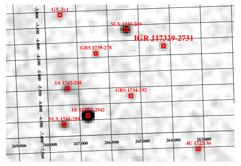
Figure 1: Zoom of the IBIS/ISGRI mosaic of the region around IGR J17329-2731, as obtained from the combined SCWs in revolutions 1850-1859 (excluding the SCW 35 in revolution 1850). The source is detected at a significance of $10\sigma$.

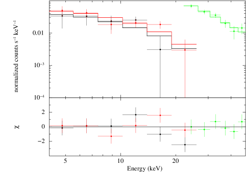
Figure 2: JEM-X1 (black), JEM-X2 (red), and ISGRI (green) spectra of IGR J17329-2731 extracted by using all combined data across revolutions 1850-1878 (excluding SCW 35 in revolution 1850). The best fit model is obtained with an absorbed power law (see text for details). The residuals from the fit are shown in the bottom panel.

Figure 3: ISGRI light curve of IGR J17329-2731 during SCW 35 (20-100 keV) showing the flare displayed by the source. The time resolution is 100 s.

We analyzed separately the INTEGRAL data obtained from SCW 35 in revolution 1850. As reported by Postel et al. (2017), the source was located at the very rim of the JEM-X FoV during the observational time covered by this SCW (2017 August 13 from 16:35 to 17:05 UTC) and not detected by this instrument. In the corresponding IBIS/ISGRI data, the average source count rate was of 7.3$\pm$1.0 cts s^-1 and the light curve extracted with 100 s resolution (Fig. 3) suggests that the source underwent a flare. The ISGRI spectrum extracted from this SCW could be well fit with a simple power law with photon index 2.9${}_{-1.3}^{+1.6}$, thus indicating no significant changes in the source spectral properties compared to the longer integration spectrum described before (to within the relatively large uncertainties).

Finally, we exploited the entire archive of the INTEGRAL data to search for possible historical detections of the source by IBIS/ISGRI. We collected a total of 15172 SCWs within which IGR J17329-2731 was located less than 12 deg away from the instrument aim point. We inspected the IBIS/ISGRI images of all SCWs and found no previous significant detections of the source. From the IBIS/ISGRI mosaic built using all these data (effective exposure 31.3 Ms), we estimated a $3\sigma$ upper limit on any hard X-ray emission from the source before its discovery of 1.3$\times$10^-12 erg cm^-2 s^-1(20-100 keV; i.e., $\sim$0.1 mCrab).

2.2 XMM–Newton data

The XMM–Newton observation of IGR J17329-2731 began on 2017-08-30 04:48 UT and lasted until 15:55 UTC (OBSID: 0795711701), providing a total exposure time of 38.7 ks for the two EPIC-MOS and 36.7 ks for the EPIC-pn. The pn was operated in timing mode, while the MOS1 was operated in full frame and the MOS2 in small window mode. Data were also collected with the two grating instruments RGS1 and RGS2, but their data were not usable given the large extinction in the direction of the source (see below). No flaring background intervals were recorded, and thus the entire exposure time could be used for the scientific analysis.

All observation data files (ODFs) were processed by using the XMM–Newton Science Analysis System (SAS 16.1) following standard procedures. The regions used for the extraction of the source spectra and light curves were chosen for all instruments to be centered on the best known position of IGR J17329-2731 (see Sect. 1). The background spectra and light curve extraction regions were chosen to lie in a portion of the instrument FoV free from the contamination of the source emission. We show in the top plot of Fig. 4 the background-corrected light curve of the source in the 0.5-12 keV energy range. The source displays a clearly regular modulation with a period of $\sim$6680 s, which we interpret as the pulse period of the compact object in IGR J17329-2731 and investigate in more detail in Sect. 2.6. The same modulation is observed in the MOS1 and MOS2 light curves. The average and peak count rate of the source along this modulation was not sufficiently high to cause any pileup in the pn and MOS2 data. However, MOS1 data were significantly affected by pileup (verified with the SAS epaplot task) and thus discarded for further analysis as they could not provide any significant improvement of the results.

In Fig. 4, we also show the energy resolved pn light curves of the source and the corresponding hardness ratio (HR). This was computed with an adaptive rebinning (see, e.g., Bozzo et al., 2013a), achieving in each soft time bin a signal-to-noise ratio (S/N) of $\gtrsim$10. No remarkable changes of the HR are recorded that could have indicated large spectral variations during the pulse phase. We thus did not perform any pulse phase or HR-resolved spectral analysis.

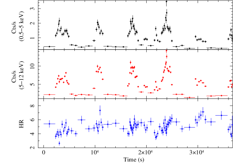
Figure 4: Top: 0.5-12 keV pn light curve of IGR J17329-2731 with a time resolution of 100 s. Bottom: The energy-resolved pn light curve of IGR J17329-2731 (top and middle panels) and the correspondingly computed HR (bottom panel).

We also extracted the pn and MOS2 spectra using the entire exposure time available. The pn and MOS2 spectra were fit together with the quasi-simultaneous NuSTAR data and the results are reported in Sect. 2.7.

2.3 NuSTAR data

IGR J17329-2731 was observed by NuSTAR from 2017 August 29 at 15:35 to August 30 at 02:36 (UTC). The Target of Opportunity observation (OBSID 90301012002) was triggered as close as possible to the XMM–Newton observation (see Sect. 2.2). After having applied to the NuSTAR data all the good time intervals (GTI) accounting for the Earth occultation and the South Atlantic Anomaly passages, we obtained an effective exposure time of 20.8 ks for both the focal plane modules A and B (FPMA and FPMB). The data were processed via nustardas v1.5.1 and the latest calibration files available (v.20171002). The source spectra and light curves were extracted from a 80 arcsec circle centered on the source, while the background products were extracted from a region with a similar extension but centered on a region free from the contamination of the source emission. Various extraction regions were also used for the source and background products to verify that none of the timing and spectral features could be affected by some specific choices (see Sect. 2.6 and 2.7).

The FPMA and FPMB light curves of the source displayed a clear modulation with a period of $\sim$6680 s (Fig. 5), similar to that observed from the XMM–Newton data (see Sect. 2.2). The timing analysis of the NuSTAR data is presented in Sect. 2.6. The FPMA and FPMB source spectra were rebinned in order to have at least 100 photons per energy bin and fit together with the XMM–Newton spectra in Sect. 2.7.

Figure 5: NuSTAR FPMA light curve of IGR J17329-2731 in the 3-60 keV energy range.

2.4 Swift data

IGR J17329-2731 was observed by the Neil Gehrels Swift Observatory (Burrows et al., 2005) from three days after the discovery up to 2017 October 26, when the source entered into a few months-long Sun constraint. The monitoring program requested from Swift provide deeper coverage during the first few weeks after the discovery (up to several 1 ks-long observations per week) and was relaxed in the following period as the source showed a relatively stable flux level and spectral properties.

The XRT data were analyzed via the standard software (Heasoft v6.22.1) and the latest calibration files available (CALDB 20170501). All data were processed and filtered with xrtpipeline (v0.13.4). The source displayed an average count rate of 0.155$\pm$0.006 cts s^-1 (0.5-10 keV) throughout the campaign and no data were significantly affected by pileup. The source events were extracted from a circular region with a radius of 20 pixels (where 1 pix corresponds to $\sim 2\aas@@fstack{\prime\prime}36$), while background events were extracted from a source-free region with a similar radius. We show in Fig. 6 the long-term background subtracted XRT light curve in the 0.5-10 keV energy band corrected for point spread function losses and vignetting. The XRT spectra extracted from each observation could be well fit with an absorbed power-law model. This more complex spectral model did not improve the fits and resulted in poorly constrained spectral parameters. A log of all XRT observations used with the corresponding spectral fit results is reported in Table 1. The marginally noticeable correlation between the measured values of the absorption column density and the power-law photon index is due to the combination of the limited statistics of the single XRT pointings and the narrow bandpass of the instrument.

Table 1: Log of all Swift/XRT observations used in the present paper. We also report for each observation the results obtained from the spectral analysis. In all cases, the best fit model is an absorbed power law (tbabs*pow in Xspec), where we used wilm abundances (Wilms et al., 2000) and vern cross sections (Verner et al., 1996). The reported flux is in the 0.5-10 keV energy range and in units of 10^-11 erg cm^-2 s^-1(it is not corrected for absorption). We note that a few adjacent observations were merged together to obtain a reasonable statistics to perform the spectral fit. All spectra were fit with the C-statistics (Cash, 1979) due to the relatively low number of counts.

Sequence	Obs.	Start time	End time	Exposure	$N_{\rm H}$	$\Gamma$	Flux${}_{\rm 0.5-10\leavevmode\nobreak\ keV}$	cstat/d.o.f.
	Mode	(UTC)	(UTC)	(s)	(1023 cm-2)
00010244001	PC	2017-08-16 02:26:50	2017-08-16 02:45:55	1973	4.9$\pm$4.0	-0.9${}^{+1.4}_{-1.6}$	2.9${}^{+0.8}_{-0.6}$	39.6/23
00010244002	PC	2017-08-16 17:03:06	2017-08-16 20:02:21
00010244003	PC	2017-08-22 03:47:02	2017-08-22 05:30:03	960	5.1${}^{+1.7}_{-1.5}$	1.6${}^{+1.1}_{-1.0}$	16.0$\pm$3.0	55.8/49
00010244004	PC	2017-08-24 16:43:09	2017-08-24 23:11:00	872	6.6${}^{+3.2}_{-2.7}$	1.4${}^{+1.7}_{-1.5}$	4.9${}^{+1.4}_{-0.9}$	28.8/26
00010244005	PC	2017-08-25 23:00:00	2017-08-26 06:39:00	601	2.5${}^{+2.8}_{-2.1}$	-0.9${}^{+1.5}_{-1.4}$	5.1${}^{+1.7}_{-1.3}$	10.7/14
00010244006	PC	2017-08-26 08:06:00	2017-08-26 14:59:00	862	5.3${}^{+4.7}_{-4.4}$	-0.4${}^{+1.7}_{-1.6}$	7.8${}^{+2.5}_{-2.0}$	13.7/15
00010244007	PC	2017-09-05 21:29:00	2017-09-05 23:17:00	659	4.2${}^{+2.8}_{-2.4}$	1.8${}^{+1.8}_{-1.6}$	3.6${}^{+1.2}_{-0.8}$	25.9/18
00010244008	PC	2017-09-10 22:35:00	2017-09-10 22:53:00	952	6.6${}^{+3.6}_{-3.1}$	1.1${}^{+1.9}_{-1.7}$	3.6${}^{+1.3}_{-0.9}$	18.0/19
00010244009	PC	2017-09-13 01:36:00	2017-09-13 06:28:00	717	8.2${}^{+4.8}_{-3.8}$	3.2${}^{+2.8}_{-2.3}$	2.7${}^{+1.2}_{-0.7}$	19.7/14
00010244010	PC	2017-09-16 12:43:00	2017-09-16 13:02:00	1100	3.3${}^{+1.4}_{-1.6}$	1.5${}^{+1.2}_{-1.1}$	3.4${}^{+0.8}_{-0.6}$	51.8/29
00010244011	PC	2017-09-23 15:10:00	2017-09-23 21:48:00	897	2.6${}^{+2.6}_{-2.5}$	0.7${}^{+1.3}_{-1.2}$	8.7${}^{+1.9}_{-1.7}$	23.3/32
00010244012	PC	2017-09-30 16:25:00	2017-09-30 16:42:00	955	6.3${}^{+2.7}_{-2.1}$	2.7${}^{+1.7}_{-1.5}$	5.1${}^{+1.5}_{-1.0}$	32.2/36
00010244013	PC	2017-10-07 01:12:00	2017-10-07 02:57:00	1508	1.6${}^{+0.8}_{-0.7}$	0.7$\pm$0.8	5.3${}^{+1.1}_{-0.9}$	72.8/44
00010244014	PC	2017-10-14 03:51:00	2017-10-14 04:03:00
00010244015	PC	2017-10-21 00:26:00	2017-10-21 01:56:00	1381	4.5${}^{+1.5}_{-1.3}$	1.5${}^{+1.0}_{-0.9}$	5.1$\pm$0.8	53.7/57
00010244016	PC	2017-10-26 12:28:00	2017-10-26 12:45:00

Figure 6: Light curve obtained from the Swift /XRT monitoring campaign performed from 2017 August 16 (57981 MJD) up to 2017 October 26 (58052 MJD). Each point of the light curve corresponds to the average count rate of the source during every XRT observation. The vertical lines indicate the mid-time of the XMM–Newton (dot-dashed line) and NuSTAR (dotted line) observations.

The XRT data showed that, following the INTEGRAL discovery, the source remained at a relatively stable X-ray flux and did not show significant spectral variability. The limited flux and spectral variability measured across the various observations are typical of wind-fed systems and in the case of IGR J17329-2731 are also related to the modulation of the X-ray emission by the long spin period of the source (see Sect. 2.6). We also fit with an absorbed power-law model the source spectrum extracted by stacking together all XRT data (effective exposure time 13.2 ks). The fit gave a poor result ($\chi^{2}_{\rm red}$/d.o.f.=1.7/78), and thus we improved the description of these data ($\chi^{2}_{\rm red}$/d.o.f.=1.1/76) adding a high energy cutoff (highecut in Xspec; see also Sect. 2.7). We measured in this case an absorption column density of (2.3$\pm$0.8)$\times$10²³ cm^-2, a power-law photon index of $\Gamma$=-0.5$\pm$0.8, a folding energy $E_{\rm fold}$=3.3${}^{+3.4}_{-1.2}$ keV, a cutoff energy of $E_{\rm cut}$=6.4$\pm$0.3 keV, and an average 0.5-10 keV flux of (4.5$\pm$0.3)$\times$10^-11 erg cm^-2 s^-1. We noticed that fixing the value of the folding energy to that measured from the combined XMM–Newton and NuSTAR data ($E_{\rm fold}$=14.5 keV) would not significantly affect the quality of the spectral fit ($\chi^{2}_{\rm red}$/d.o.f.=1.1/77). Furthermore, the other parameters would be in good agreement with those reported in Sect. 2.7. In particular, we obtained in this case $\Gamma$=0.5$\pm$0.3, $N_{\rm H}$=(3.3$\pm$0.5)$\times$10²³ cm^-2, and $E_{\rm cut}$=6.4$\pm$1.4 keV. This further confirmed that the source did not undergo significant spectral variations during the entire observational period monitored with Swift, XMM–Newton, and NuSTAR.

2.5 ROSAT data

A ROSAT/PSPC (Pfeffermann et al., 1987) observation was carried out in the direction of IGR J17329-2731 on 1992 February 29 for a total exposure time of 3.7 ks. The processed image in the 0.1-2.4 keV energy range was downloaded from the HEASARCH archive, together with the corresponding exposure map. IGR J17329-2731 was not detected in this observation and we determined a $3\sigma$ upper limit on the source count rate of 0.003 Cts s^-1 via the tool sosta available within ximage (heasoft v.6.22.1). We converted this count rate into a flux using the online webpimms tool and assuming a spectral model comprising an absorption column density of 5$\times$10²³ cm^-2 and a power law with a photon index ranging between $\Gamma$=0.5 and $\Gamma$=3.0 (see Table 1). Because of the limited energy coverage of the instrument and the strong absorption local to the source, we obtained unconstraining $3\sigma$ upper limits on the 0.5-10 keV flux within the range (0.4-7)$\times$10^-4 erg cm^-2 s^-1.

2.6 XMM–Newton and NuSTAR timing analysis

Given the evident modulation of the source light curve in the XMM–Newton data, we first corrected the arrival times of the photons recorded by the pn camera to the solar system barycenter using the best available position of the source and then carried out a detailed timing analysis. We created a Lehay-normalized power density spectrum (PDS) with Nyqvist frequency of 1024 Hz by averaging $\sim$16ks data intervals. The PDS shows a prominent feature at $\sim$6680 s and a second peak at twice this value. We interpret these features as the pulse period of the source and its harmonic. To further investigate this periodicity, we performed epoch-folding search of the whole XMM–Newton observation using 80 phase bins and exploring the frequency space around the value obtained from the analysis of the PDS with steps of 10^-7 Hz for a total of 1001 steps. The best X-ray pulse profile is obtained using a period of 6692$\pm$4 s (1 $\sigma$ c.l.). To estimate the uncertainty on the period we performed Monte Carlo simulations by generating 100 datasets with equal exposure, count rate, and pulse profile as the observed data. For each of these datasets, we then applied the same procedure described above to obtain the best period value of the periodicity. Finally, we estimated the period uncertainty as the standard deviation of the best period values distribution.

We also investigated the average pulse profile as a function of energy by dividing the XMM–Newton energy range in four intervals characterized by roughly the same number of photons. Figure 7 shows the average pulse profiles for the selected energy bands. No significant differences are observed within the energy range covered by the pn. Finally, we estimated the pulse fraction $f$ as a function of energy selecting 11 statistically equivalent intervals (see Fig. 8) with the equation

$$f=\frac{max(P)-min(P)}{max(P)+min(P)},$$ (1)

where $P$ is the pulse profile. The choice of statistically equivalent intervals allowed us to ensure that the measured changes of $f$ as a function of energy are an intrinsic property of the source. Our findings suggest that the pulse fraction increases as a function of energy, and there is an indication of a possible decrease around the fluorescence iron line energy ($\sim$6.4 keV, see below). This is similar to what is observed in other X-ray pulsars and particularly in wind-fed systems (see also Sect. 4).

Figure 7: Pulse profiles of IGR J17329-2731 as determined from the EPIC-pn data. The best determined pulse period used to obtain the profiles is 6692$\pm$4 s (1 $\sigma$ c.l.).

Figure 8: Pulsed fraction as a function of the energy derived from the EPIC-pn data.

As the NuSTAR data are affected by regular interruptions due to the occultation of the source by the Earth, we used a different technique to determine the best source period. The source FPMA and FPMB light curves with 100 s resolution (3-60 keV) were first normalized to the corresponding average count rates, combined together, and then modeled with a Bayesian approach to derive the posterior distribution of the fitting parameters. We assumed as a baseline model a constant plus four Fourier harmonics, such that the total number of parameters are the constant $D$, the relative amplitudes and phases of the harmonics ($A_{i}$ and $\phi_{i}$), and the spin period $P$. To prevent boundary issues, amplitudes were varied from zero to one and phases from zero to 1.5. The intrinsic source variability was accounted for in the method by multiplying the amplitudes of the Fourier harmonics by a factor sampled from a normal distribution centered at unity (represented as $\xi$ below). In addition, we introduced an overall intrinsic scatter in the source emission by sampling its count rate from a normal distribution centered on the expected value. The amplitudes of these distributions are indicated as $\sigma_{p}$ and $\sigma$ and are parameters of the model with a non-constraining prior. To summarize, the model can be expressed as $\mathcal{N}(c,\sigma)$, where

$$c=D\left[1+2\xi\sum_{i=1}^{4}A_{i}\cos\left(2\pi\left(i\frac{t}{P}-\phi_{i}\right)\right)\right]$$ (2)

and

$$\xi=\mathcal{N}(1,\sigma_{p}).$$ (3)

In the equation above, $\mathcal{N}(m,s)$ represents a normal distribution with mean $m$ and standard deviation $s$. We used a Gibbs sampler from JAGS and three chains for consistency. Following a burn-in phase of 2000 realizations, we sampled 1000 elements from each chain with a length of 10000 realizations. We inspected the parameter distribution and found no significant degeneracies between them. The best spin period obtained with this method is 6696$\pm$15 s at $1\sigma$ c.l., and we measured a variability of the total source emission of $\sigma$=59$\pm$4% (all uncertainties here are given at $1\sigma$ c.l.). The parameter $\sigma_{p}$ could not be constrained in the fit and was fixed to 0, verifying that this did not significantly affect the results. The same technique applied to the XMM–Newton data provided a period that is compatible with that reported above (6694$\pm$13 s). In the case of the XMM–Newton data we measured from the fit $\sigma_{p}$=39$\pm$4% and $\sigma$=86$\pm$7%.

We also adopted for further confirmation a third technique, fitting both the XMM–Newton and NuSTAR light curves with a superposition of sinusoidal function with periods harmonically related $f(x)$=$a$+$\sum_{n=1}^{13}$$b_{n}$$\sin{\left(\frac{2\pi(t-\phi_{n})}{nP}\right)}$, where $a$, $b_{n}$, and $\phi_{n}$ represent a constant, the amplitude, and the time phase of the sinusoidal functions. We obtained a spin period of $6688\pm 4$ s (1 $\sigma$), $6675\pm 5$ s (1 $\sigma$), and $6680\pm 3$ s (1 $\sigma$) for XMM–Newton, NuSTAR, and the two datasets combined; in the combined fit, we only forced the period to be the same among the two datasets but left all other parameters free to vary (Fig. 9). These values are well in agreement with the periods determined through the various techniques above and we thus consider in the following the last value as our best and most accurate estimate of the pulse period from IGR J17329-2731.

We show in Fig. 10 the source energy-resolved folded pulse profiles obtained from the NuSTAR data, using the most accurate period determined so far of 6680$\pm$3 s. We only show FPMA data, but equivalent results were obtained from the FPMB; the phase 0 was set to 57994 MJD. There seem to be no remarkable differences between the lower (3-20 keV) and higher energy (20-60 keV) pulse profiles. We also could not find noticeable differences by changing the energy bands of these profiles slightly.

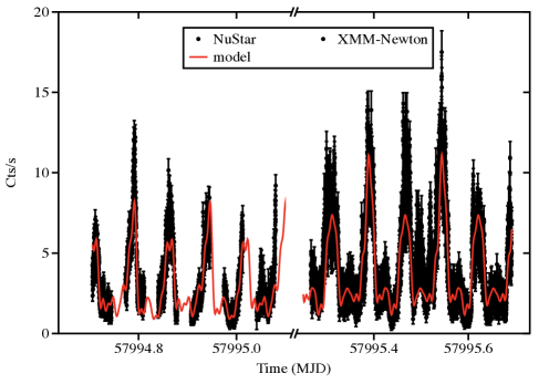
Figure 9: Results of the fit to the XMM–Newton (right side of the timeline) and NuSTAR (left side of the timeline) light curves of IGR J17329-2731 with a superposition of sinusoidal functions with harmonically related periods. The red curve represents the best fit model and the most accurately derived spin period of the source from the combined XMM–Newton + NuSTAR dataset is $6680\pm 3$ s (1 $\sigma$).

Figure 10: Pulsed profiles obtained from the NuSTAR FPMA data in various energy ranges (3-20 keV and 20-60 keV). The profiles were obtained from the source light curves folded on the best determined pulse period of 6680$\pm$3 s (1 $\sigma$).

2.7 XMM–Newton and NuSTAR combined spectral analysis

In this section, we report on the detailed broadband spectral analysis of the X-ray emission from IGR J17329-2731, exploiting the quasi-simultaneous XMM–Newton and NuSTAR data. These spectra could not be described by a simple absorbed power-law model ($\chi^{2}_{\rm red}$/d.o.f.=7.89/1051), where large residuals were left at both the lower and higher ends of the covered energy range, and around 6-7 keV (see Fig. 11).

We improved the fits using a number of different phenomenological models. The best description of the source continuum emission was achieved with an absorbed power-law including a cutoff at the higher energies and a partial absorber (const*tbabs*tbpcf*highecut*pow in Xspec, where $const$ is a normalization constant included to take into account inter-calibration uncertainties between the different instruments and the fact that the data were not strictly simultaneous). We used wilm abundances and vern cross sections. The value of the first absorption column density was fixed to 3$\times$10²¹ cm^-2, which agrees with the expected Galactic value in the direction of the source. We included three Gaussians in the fit to take into account the presence of evident emission lines at 2.3 keV, 6.4 keV and 7.1 keV, together with a partial covering model to take into account the residuals below 2 keV (spectral model 1 in Table 2). The three emission lines correspond to the S K$\alpha$, Fe K$\alpha$, and Fe K$\beta$, respectively (see, e.g., Fürst et al., 2011, and references therein).

As can be seen from Fig. 11, this model has not yet provided an acceptable result ($\chi^{2}_{\rm red}$/d.o.f=1.74/1037). In particular, residuals resembling the shape of absorption features were still left around $\sim$20 keV, $\sim$30 keV, and $\sim$40 keV. We verified that these residuals could not be decreased with alternative source and background extraction regions, leading to the conclusion that they are intrinsic to the source. To the best of our knowledge, there are no instrumental features at the energies of the identified absorption lines. We thus included a first absorption feature (gabs in Xspec) at 20 keV, significantly improving the fit up to $\chi^{2}_{\rm red}$/d.o.f.=1.25/1035. A second gabs component at 30 keV further improved the fit up to $\chi^{2}_{\rm red}$/d.o.f.=1.16/1033. A third gabs component with a centroid energy around $\sim$40 keV led only to a marginal improvement of the fit ($\chi^{2}_{\rm red}$/d.o.f.=1.14/1031). In the final fit we fixed the widths of the three gabs components to the best fit values obtained by the previous fits to avoid continuum modeling with the absorption features (this is a common practice for similar fits of complex X-ray pulsar spectra; see, e.g., Ferrigno et al., 2009; Müller et al., 2013). We verified that leaving these parameters free to vary in the fit did not significantly affect the results. A nearly equivalent fit could be obtained by changing the partial covering component with a low temperature blackbody (diskbb in Xspec). As the low energy turnover of the XMM–Newton and NuSTAR spectra was characterized by an evidently different curvature, we left free to vary in the fit either the partial covering fraction or the normalization of the disk blackbody component between the two datasets. The normalization of the 6.4 keV iron line was also significantly different between XMM–Newton and NuSTAR, and thus left free to vary in the fit. We report all the results of the spectral fits in Table 2. In all cases, the normalization constants turned out to be compatible with unity and are thus not reported explicitly in the table.

For completeness, we also performed a fit to the broadband spectrum using the cyclabs component in Xspec instead of the three gabs components. This model provided an equivalently good fit to the data, but the width of the fundamental line (now centered at 19.7${}^{+0.3}_{-0.7}$ keV) and the first harmonic turned out to be rather large (8.9${}^{+0.3}_{-0.8}$ keV and 12.7${}^{+3.3}_{-4.7}$ keV, respectively). On the one hand, it is interesting to note that only two lines in harmonic ratio are required with this alternative model (no residuals are left around 30 keV). On the other hand, the two broad features seem to be used by the Xspec fit routine to cover a large portion of the source continuum emission and thus we did not consider the model with a cyclabs component as a convincingly viable alternative.

A number of other models were tested as well, including a combination of a partial covering with a blackbody (bbodyrad in Xspec) and a Comptonized plasma model (comptt in Xspec). In the first case, indicated as “Model 2” in Table 2, the blackbody radius turns out to be unphysically too low for this component to be associated with the emission from an accretion disk around the compact object in IGR J17329-2731 (see Sect. 4). For the model using a comptt component, indicated as “Model 3” in Table 2, we linked in the fit the temperature of the bbodyrad component to be the same between the XMM–Newton and NuSTAR data, while the normalization of this component was left free to vary among the two datasets. As the comptt covers mainly the high energy part of the spectrum, all component parameters were linked between the XMM–Newton and NuSTAR data. In this model, the bbodyrad component has a hot temperature ($\sim$1.4 keV) and a small radius ($\lesssim$1 km), suggesting a hot spot origin on the NS surface. The seed photon temperature needed in order for the comptt component to cover properly a large fraction of the source hard continuum emission is much larger than that of the bbodyrad component, and linking the two temperatures did not result in an acceptable fit (featuring “S” shaped residuals). The comptt component is usually adopted to describe the Comptonized emission in the accretion columns of X-ray pulsars, and it cannot be excluded that the seed photons have a different origin with respect to the NS hot spot or could be part of these photons already up-scattered to higher energies. The drawback of this assumption is that the resulting plasma temperature of the model is roughly an order of magnitude higher ($kT$$\sim$120 keV) than what is usually observed in other X-ray pulsars and especially in symbiotic X-ray binaries observed with instruments providing a wide X-ray energy coverage (see, e.g., Masetti et al., 2007b; Enoto et al., 2014; Kitamura et al., 2014). The interesting outcome of the fit with this alternative model is that only the gabs component at $\sim$21 keV remains highly significant, while residuals at $\sim$40 keV are barely noticeable. The addition of a gabs component at $\sim$40 keV only led to a marginal improvement of the fit from $\chi^{2}_{\rm red}$/d.o.f.=1.16/1031 to $\chi^{2}_{\rm red}$/d.o.f.=1.15/1029, but still permitted us to get rid of the residuals above $\sim$40 keV (see Fig. 12). No residuals were left around $\sim$30 keV, thus excluding the presence of the third gabs component required in the fit with the highecut*pow. We thus conclude that the gabs component at $\sim$30 keV is likely model-dependent, and should be investigated further with deeper NuSTAR observations of the source. Depending on the specific model considered, we measured a ratio of the normalization of the Fe K$\beta$ to Fe K$\alpha$ lines ranging from 0.20 to 0.23, in agreement with the expectations for neutral iron (Palmeri et al., 2003). The measured equivalent widths of the Fe K$\alpha$ feature is also in line with the expected values for highly absorbed high mass X-ray binaries and other SyXBs (Giménez-García et al., 2015).

We also attempted a pulse phase-resolved spectral analysis of the NuSTAR data to search for possible changes in at least the main absorption feature at $\sim$21 keV. We extracted the spectra during the phase intervals 0.5-0.8 and 0.0-0.2 in Fig. 10, i.e., corresponding to the most prominent and the secondary peak of the source pulse profile. We could not find evidence for significant spectral changes, although the statistics of the NuSTAR spectrum extracted during the secondary peak was far too low to perform a detailed investigation.

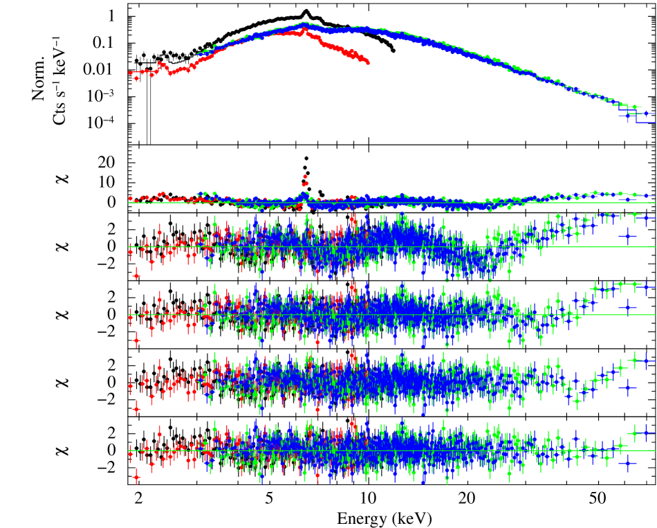
Figure 11: Quasi-simultaneous XMM–Newton and NuSTAR spectra of IGR J17329-2731. The EPIC-pn is in black, the EPIC-MOS2 in red, the FPMA in green, and the FPMB in blue. The best fit to the data is obtained with the model const*tbabs*tbpcf*gabs*gabs*gabs* (gaussian+gaussian+gaussian+highecut*powerlaw). The residuals from the best fit are shown in the bottom panel. The second panel from the top shows the residuals obtained using a simple absorbed power law with a high energy cutoff (tbabs*highecut*powerlaw). The third panel from the top shows the residuals obtained using a simple absorbed power law with a high energy cutoff and the three lines at 2.3 keV, 6.4 eV, and 7.1 keV (tbabs*(gaussian+gaussian+gaussian+highecut*powerlaw)). The fourth panel from the top shows the residuals obtained by including a gabs component with a centroid energy of $\sim$20 keV, while the fifth panel reports the residuals obtained when a second gabs component with a centroid energy of $\sim$30 keV is accounted for in the model as well.

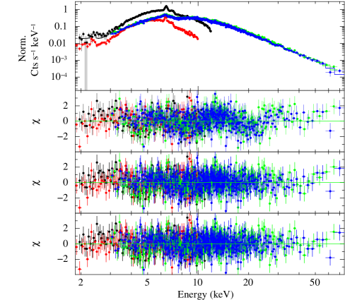
Figure 12: Same as Fig. 11 but in the case of the best fit model obtained with a combination of a partial covering, a hot bbodyrad, and a comptt component (plus the three Gaussians at 6.4, 7.1, and 2.3 keV). The residuals in the second panel from the top correspond to the case in which no gabs is included in the fit, while those in the third panel from the top show the improvement obtained by including in the fit an absorption feature around 21 keV. The bottom panel shows the residuals from the best fit, where a possible second absorption component around 40 keV wa included in the model as well.

Table 2: IGR J17329-2731 broadband spectral analysis results. Model 1 is const*tbabs*tbpcf*gabs*gabs*gabs*(gauss+gauss+gauss+ highecut*pow), whereas model 2 is const*tbabs*gabs*gabs*gabs*(diskbb+gauss+gauss+gauss+ highecut*pow). Model 3 corresponds to the case const*tbabs*tbpcf*gabs*gabs*(gauss+gauss+gauss+ bbodyrad+Comptt). The parameter $N_{\rm H1}$ is the Galactic absorption column density and $N_{\rm H2}$ the local absorption. The parameter $f$ is the partial covering fraction. Parameters kT_BB and R_BB are the temperature and radius of the diskbb/bbodyrad component (the latter is given assuming a distance of 2.7 kpc and in the diskbb case also considering a face-on disk). The parameter $\sigma$ is the width of the cyclotron absorption features and $\tau$ their strength. The centroid energy and the equivalent width (Eqw) of all Gaussian emission line are reported. The parameter $\Gamma$ is the photon index and E_cut, E_fold the parameters of the high energy cutoff. Parameters kT_seed, kT, and $\tau_{\rm p}$ are the Comptt component. Fluxes are given in the 0.5-10 keV (measured from the XMM–Newton spectra) and in the 3-79 keV energy band (measured from the NuSTAR data) with units of 10^-11 erg cm^-2 s^-1. Values in parentheses are those determined from the NuSTAR data and untied during the simultaneous fit with the XMM–Newton data.

Parameter	Model 1	Model 2	Model 3
$N_{\rm H1}$ (1022 cm-2)	0.3 (fixed)	48.9${}^{+0.3}_{-0.4}$	0.3 (fixed)
		(38.8${}^{+1.1}_{-0.7}$)
$N_{\rm H2}$ (1022 cm-2)	47.4$\pm$0.3	—	48.4$\pm$0.5
$f$	0.9965$\pm$0.0005	—	0.9946$\pm$0.0006
	(0.892$\pm$0.005)	—	(0.902${}^{+0.005}_{-0.009}$)
kTBB (keV)	—	0.28${}^{+0.01}_{-0.02}$	1.41${}^{+0.07}_{-0.1}$
RBB (km)	—	62${}^{+18}_{-5}$	0.35$\pm$0.05
		(133${}^{+41}_{-6}$)	(0.38$\pm$0.03)
$E_{\rm cycl1}$ (keV)	20.9$\pm$0.2	21.1$\pm$0.2	21.6$\pm$0.2
$\sigma_{\rm cycl1}$ (keV)	4.0 (fixed)	4.0 (fixed)	4.6$\pm$0.2
$\tau_{\rm cycl1}$	3.6$\pm$0.2	3.7$\pm$0.7	4.4${}^{+3.4}_{-0.2}$
$E_{\rm cycl2}$ (keV)	31.6${}^{+0.6}_{-0.7}$	32.3$\pm$0.9	37.7${}^{+1.8}_{-7.5}$
$\sigma_{\rm cycl2}$ (keV)	7.0 (fixed)	7.0 (fixed)	7.0 (fixed)
$\tau_{\rm cycl2}$	9.1$\pm$0.5	9.0$\pm$0.5	3.8${}^{+1.5}_{-0.8}$
$E_{\rm cycl3}$ (keV)	44.0$\pm$1.2	44.4$\pm$1.2	—
$\sigma_{\rm cycl3}$ (keV)	4.0 (fixed)	4.0 (fixed)	—
$\tau_{\rm cycl3}$	4.3${}^{+1.0}_{-0.9}$	4.2${}^{+1.0}_{-0.9}$	—
$E_{\rm FeK\alpha}$ (keV)	6.444$\pm$0.005	6.450$\pm$0.002	6.450${}^{+0.003}_{-0.010}$
$Eqw_{\rm FeK\alpha}$ (keV)	0.19$\pm$0.01	0.19$\pm$0.01	0.19$\pm$0.05
	(0.15$\pm$0.03)	(0.15$\pm$0.02)	(0.14$\pm$0.04)
$E_{\rm FeK\beta}$ (keV)	7.104$\pm$0.008	7.104$\pm$0.008	7.099$\pm$0.005
$Eqw_{\rm FeK\beta}$ (keV)	0.049${}^{+0.005}_{-0.017}$	0.049${}^{+0.003}_{-0.016}$	0.052${}^{+0.005}_{-0.012}$
$E_{\rm SK\alpha}$ (keV)	2.33$\pm$0.03	2.33${}^{+0.01}_{-0.02}$	2.36${}^{+0.03}_{-0.02}$
$Eqw_{\rm SK\alpha}$ (keV)	0.51${}^{+0.06}_{-0.27}$	2.1${}^{+13.9}_{-0.5}$	0.32${}^{+0.29}_{-0.08}$
Ecut (keV)	5.8$\pm$0.1	5.7$\pm$0.1	—
Efold (keV)	14.5$\pm$0.3	14.9$\pm$0.2	—
$\Gamma$	0.58${}^{+0.03}_{-0.06}$	0.60${}^{+0.03}_{-0.01}$	—
kT (keV)	—	—	120.6${}^{+4.7}_{-1.5}$
kTseed (keV)	—	—	3.2${}^{+0.4}_{-0.2}$
$\tau_{\rm p}$	—	—	0.030${}^{+0.10}_{-0.003}$
$F_{\rm 0.5-10keV}$	6.38${}^{+0.02}_{-0.10}$	6.38${}^{+0.01}_{-0.11}$	6.38${}^{+0.10}_{-0.25}$
$F_{\rm 3-79keV}$	34.5${}^{+0.3}_{-1.0}$	34.5${}^{+0.5}_{-0.9}$	35.3${}^{+1.0}_{-1.9}$
$\chi^{2}_{\rm red}$/d.o.f	1.15/1031	1.17/1029	1.16/1030

3 Optical data

We obtained two spectra of the source with the Goodman Spectrograph (Clemens et al., 2004) on the SOAR telescope, using a 0.95^′′ slit in both cases. The first spectrum was acquired on 2017 August 25.099 for a total exposure time of 900 s and used the 400 l mm^-1 grating, covering the wavelength range 4800–8820 Å and providing a resolution of 5.6 Å. The second spectrum was obtained on 2017 August 31.097 (total exposure time 1200 s), using a higher resolution 2100 l mm^-1 grating, which provides a wavelength coverage between 6140–6700 Å and a resolution of 0.75 Å. Both spectra were analyzed with standard techniques. The 400 l mm^-1 spectrum was calibrated in flux using a first order correction for slit losses and scaled using the $i^{\prime}$ magnitude at a similar epoch of that reported by Russell et al. (2017) using photometric measurements.

3.1 Spectral analysis

The broadband optical spectrum of IGR J17329-2731 contains multiple emission lines, of which the most evident is the H$\alpha$ line (Fig. 13). The high resolution spectrum shows that this line is clearly double peaked (Fig. 13). To estimate the properties of the observed H$\alpha$ feature in our spectrum, we deblended the peaks by fitting two profiles on top of a continuum. We note that the extended wings of the features are better described by Lorentzian profiles rather than Gaussian profiles. We estimate a peak separation of 113$\pm$2 km s^-1. The wings of the feature are significantly broad extending at least $\sim$2500 km s^-1 from the rest wavelength and are difficult to estimate accurately. The double-peaked H$\alpha$ line strongly suggests the presence of an accretion disk around the compact object.

The broadband spectrum shows strong TiO bands, typically observed from late M stars. The sharp TiO band at $\sim$8200 Å allows us to classify the star as a M giant and rule out the M dwarf case. The spectrum is fully consistent with that expected from an M giant even above 7500 Å, but it shows a brighter continuum than expected for an M giant in the bluer part with only marginal evidences of TiO bands. This could be related to the contribution from the accretion disk. In order to test this hypothesis and simultaneously constrain the temperature of the companion, we created a spectral model comprising a synthetic stellar component based on the Phoenix models (Husser et al., 2013) and an accretion disk. The effect of reddening on the complete model was also included. This model provided a good match with the observations, proving that the accretion disk is the dominant component at $<$7500 Å and suggesting a temperature of the companion of $\sim$3000 K (Fig. 13). This is compatible with a late M giant star (Houdashelt et al., 2000). We also estimated E(B-V)$\sim$3. This value is much lower than that derived from the estimated extinction in X-rays ($\sim$46), even considering the most recently determined empirical correlations between E(B-V) and $N_{\rm H}$ (Foight et al., 2016; Bahramian et al., 2015). As it is commonly the case in strongly obscured X-ray binaries, this confirms that the absorption is local to the source (see, e.g., Walter et al., 2003; Filliatre & Chaty, 2004; Chaty & Rahoui, 2012).

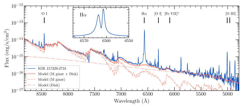
Figure 13: SOAR Goodman spectrum of IGR J17329-2731, together with a model comprising an M giant star based on Phoenix models (Husser et al., 2013) plus an accretion disk. The model spectrum was reddened assuming E(B-V)$\sim$3. The inset shows the double-peaked H$\alpha$ as seen in the high resolution spectrum, indicating the presence of an accretion disk around the compact object in IGR J17329-2731. 

The SOAR spectra also allowed us to constrain the radial velocity of the identified oxygen and iron emission lines, leading to an estimate of IGR J17329-2731 heliocentric radial velocity of $116\pm 6$ km $s^{-1}$.

3.2 Distance to the source

The identification of the optical counterpart to IGR J17329-2731 in the Faulkes and SOAR observations also allowed us to confirm the association of the infrared counterpart from the 2MASS catalog 2MASS 17325067-2730015 with magnitudes J=9.823, H=8.436, and K=7.775. As IGR J17329-2731 was never detected in X-rays before August 2017, we assume that the 2MASS magnitudes were measured during quiescence and thus are dominated by the emission from the companion star. The absolute magnitudes of a late M giant are not well constrained, but available estimates suggest $M_{K}\sim-5.5$ (Nikolaev & Weinberg, 2000). From the E(B-V) value estimated above, we thus obtain $A_{K}\sim 1.14$ (e.g., see McCall, 2004) and a distance to the source of $\sim$2.7 kpc. This value has to be taken with caution, given the limited knowledge on the absolute magnitudes of M giant stars and the relatively large uncertainties affecting the reddening of IGR J17329-2731. Assuming a conservative range for E(B-V), spanning from 1.0 to 4.0, and for M_K, spanning from -4.5 to -6.5, we conclude that the uncertainty associated with our estimate of the distance to the source is 2.7${}^{+3.4}_{-1.2}$ kpc.

4 Discussion

In this paper, we reported on the data obtained from the multiwavelength campaign triggered after the discovery of the INTEGRAL transient IGR J17329-2731. The analysis of the SOAR/GOODMAN data acquired by pointing at the optical counterpart of the source reported by Russell et al. (2017) led to the identification of a M6 III star at a distance of 2.7${}^{+3.4}_{-1.2}$ kpc, thus classifying IGR J17329-2731 as a new member of the so-called symbiotic X-ray binaries (SyXBs).

These systems are rare low mass X-ray binaries (LMXBs) and in some of these systems a highly magnetized ($\gtrsim$10¹² G) NS is accreting from the slow wind of its giant companion. These systems are characterized by the longest orbital periods among the known LMXBs (several tens to thousand days) and remarkably slow pulse periods that range from hundred of seconds to hours. About ten objects were discovered in this class so far (Masetti et al., 2006, 2007a, 2007b; Nucita et al., 2007; Corbet et al., 2008; Nespoli et al., 2008; Marcu et al., 2011; Bozzo et al., 2013b; Enoto et al., 2014; Bahramian et al., 2014). Detailed evolutionary studies on the formation channels leading to syXBs were presented by Postnov et al. (2010); Lü et al. (2012); Kuranov & Postnov (2015). These studies were particularly focused on the necessary conditions to develop the long spin periods.

The general assumption is that the progenitor of a SyXB is a binary system initially hosting a NS, endowed with a moderately strong magnetic field (a few $\times$10¹² G) and a spin period $\sim$0.01 s, and a low mass main sequence star ($\lesssim$2 M_⊙) in a wide orbit (hundred of days). In the early stages of the evolution, the secondary star is in the first giant branch but does not fill its Roche lobe, leading to a negligible mass transfer toward the NS and thus to negligible high energy emission. When this is no longer the case, the interaction of the NS with the surrounding material produces substantial changes in the observable properties of the system. As the magnetic field of the NS has not decayed and its rotational velocity is still high owing to the low spin period, the system enters in a so-called propeller phase where material is ejected from the vicinity of the NS by the centrifugal force at the magnetospheric boundary. This occurs at the expense of the rotational energy, inducing a rapid increase of the NS spin period. Depending on a number of still poorly known parameters, the rate at which the NS spins down and the resulting high energy emission due to the friction with the material lost by the secondary star can vary by a factor of several (Davies & Pringle, 1981; Bozzo et al., 2008; Shakura et al., 2012). But it is relatively well understood that under these circumstances the NS can reach spin periods as long as $\gtrsim$10000 s. As little to no accretion is taking place in this stage, the system is still hardly detectable in the X-ray domain. The situation changes when the NS is slowed down sufficiently to reduce the centrifugal force at the magnetospheric boundary and allow some accretion to take place, finally shining as a SyXB. In this phase, accretion is still likely to take place directly from the stellar wind. As this is endowed with little to no angular momentum, the spin period of the NS is still expected to increase because of the effect of the friction between the relatively large magnetosphere and the surrounding dense environment. While the M giant climbs the first giant branch, the velocity of its stellar wind decreases to a level at which the formation of an accretion disk around the compact object is inevitable (Wang, 1981). Accretion in this phase leads to rapid decrease of the NS spin period and the system ceases to resemble a SyXB. At this stage, the system is few 10⁹ yr old and moves toward a configuration that resembles more a common LMXB with a fast spinning compact object (see Fig. 1 of Lü et al., 2012).

The classification of IGR J17329-2731 as a SyXB with a NS accretor is strongly supported by the results of the X-ray data analysis. The prominent periodic modulation detected in both the XMM–Newton and NuSTAR data with a period of $\sim$6680 s can be interpreted as the NS spin, which is in the expected range for a SyXB (see, e.g., the cases of 4U 1954+31 and IGR J16358-4726; Corbet et al., 2008; Patel et al., 2004). The energy resolved pulse profiles of IGR J17329-2731 are strongly reminiscent of those observed in other SyXB (see, e.g., the case of 4U 1954+31, showing structured pulses and a pulse fraction as high as 60-80%; Enoto et al., 2014) and high mass X-ray binaries hosting highly magnetized compact objects. In all these systems, the NS magnetic field dominates the dynamic of the accretion flow close to the compact star surface and the X-ray emission produced by the accretion is reprocessed within the accretion column(s) before reaching the observer (see, e.g., Caballero & Wilms, 2012, for a recent review). The structured pulse profiles can thus give an indication of the topology of the NS magnetic field, even though the inversion between the pulse profile and the configuration of the magnetic field is often very complex (see, e.g., Schönherr et al., 2007). The high pulse fraction measured from the XMM–Newton data ($\gtrsim$70%) would also be compatible with that expected in case of a highly magnetized NS.

Additional indications supporting the presence of a NS accretor in IGR J17329-2731 are obtained from the spectral analysis of the XMM–Newton, NuSTAR, and INTEGRAL data. The fits to these data revealed that the relatively hard continuum, extending up to $\sim$80 keV, could be well fit with a model featuring a power law and a high energy cutoff, and have values similar to those used for other SyXBs (see, e.g., the broadband spectral fits to the X-ray emission of 4U 1954+31 reported in Masetti et al., 2007b; Enoto et al., 2014) and binary systems hosting strongly magnetized NS (see, e.g., Walter et al., 2015, and references therein). The prominent and thin neutral iron K$\alpha$ and K$\beta$ lines are typical of wind-fed systems and are produced by the fluorescence of the X-rays due to the accretion onto the stellar wind material surrounding the compact object. The bulk of this material is usually spread around the entire binary, and thus often not sufficiently heated up to lead to the detection of emission lines due to more ionized iron states. We note that the hint in Fig. 8 of a lower pulsed fraction at energies comparable to that of the fluorescence lines further supports this conclusion. The source spectrum was also characterized by the presence of an evident line at 2.3 keV, which was interpreted as being the S K$\alpha$ line and it was already observed in a number of other wind-fed binaries with NS accretors (see, e.g., Fürst et al., 2011, and references therein). The soft excess at energies $\lesssim$2 keV could be equally fit with either a partial covering model or a disk blackbody component. The partial covering model is commonly used in wind-fed system and SyXBs (see, e.g., Masetti et al., 2007b) to describe a portion of the X-ray radiation that escapes the local absorption due to the inhomogeneous stellar wind environment and is affected only by the Galactic extinction in the direction of the source (see, e.g., Martínez-Núñez et al., 2017). The parameter $f$ in this model represents the fraction of the total radiation that escapes the local absorption, and the fact that we measured a significant change in $f$ between the non-simultaneous XMM–Newton and NuSTAR data (see Table 2) is compatible with the idea that the accretion environment around the NS changes on short timescales and is mostly regulated by the physical conditions of the stellar wind. A similar conclusion applies in case the alternative model with a blackbody component coming from the hot spot of the NS and a Comptonized component from the NS accretion column(s) is considered. This model is widely used in case of strongly magnetized pulsars (see, e.g., Walter et al., 2015, and references therein), and also requires the presence of a partial covering with a variable parameter $f$ between the XMM–Newton and NuSTAR data (although in this case the changes are less prominent).

Another important property of the source revealed by the X-ray spectral analysis is the presence of cyclotron lines. The absorption feature around $\sim$21 keV is far the most prominent in the spectrum, and our fits revealed that it is unlikely to originate from a non-optimal fit of the continuum. If this absorption feature is interpreted as the fundamental cyclotron harmonic, then we can use the centroid energy obtained from the fit to estimate the NS magnetic field $B$ with the equation $B$/(10¹² G)=$E_{\rm cycl}$/11.6 keV$\times$(1+z), where $(1+z)$ is the gravitational redshift (for a standard NS with a mass of 1.4 M_⊙ and a radius of 10 km, z$\simeq$0.3; see, e.g., Caballero & Wilms, 2012). In the case of IGR J17329-2731, we can thus estimate that $B$$\simeq$2.4$\times$10¹² G is compatible with the value expected for a SyXB. Our spectral fit revealed two other possible absorption features at energies $\sim$30 keV and $\sim$40 keV. The statistics of the NuSTAR data at these energies is far from optimal, but we checked that residuals resembling two absorption features are left at these energies even when different choices of the background and source extraction regions are considered. We cautioned, however, that these two additional features are likely model-dependent and should be confirmed by future NuSTAR observations with a better S/N; the feature at $\sim$40 keV was only marginally required in the alternative fit with the hot bbodyrad and the comptt component and no significant residuals were found in this fit around $\sim$30 keV. If we interpret these features as additional cyclotron lines, we might be observing the first harmonic of the fundamental line ($\sim$40 keV) and another cyclotron feature that is not in harmonic ratio with the others ($\sim$30 keV). Although this is not always observed in accreting X-ray pulsars, there is at least one other example where cyclotron features at independent energies were found and ascribed to the presence of emission arising in distinct regions (e.g., two regions at different heights from the compact object surface in the same accretion column or two accretion columns; Iyer et al., 2015). Future NuSTAR observations endowed with a higher S/N will be helpful to confirm the detection of all absorption features and study in more detail the possibly complex topology of the magnetic field in IGR J17329-2731. Although the feature at 30 keV remains to be investigated, at the best of our knowledge, IGR J17329-2731 is the first SyXB for which a direct measurement of the NS magnetic field is reported.

The presence of a disk around the compact object in IGR J17329-2731 is suggested by the optical spectrum (see Sect. 3.1), but we could not find strong evidence for the presence of this disk in the source X-ray spectrum. We included for completeness in Table 2 the fit to the source X-ray spectra including a diskbb component in place of the partial covering, but the latter model remained slightly more statistically preferable. Assuming the most probable distance to the source of 2.7 kpc and using the 3-79 keV X-ray flux reported in Table 2, we can estimate that at the time of the XMM–Newton and NuSTAR observations the luminosity of the source was $L_{\rm X}$=3$\times$10³⁵ erg s^-1 and thus the mass accretion rate onto the NS was $\dot{M}$$\simeq$$L_{\rm X}$$R_{\rm NS}$/(G$M_{\rm NS}$)$\sim$1.6$\times$10¹⁵ g s^-1. The measurement of the NS magnetic field provided by the cyclotron line discussed above would imply an accretion disk truncated around $R_{\rm M}$$\sim$1.6$\times$10⁹ cm (see, e.g., Bozzo et al., 2009, and references therein). This is hardly compatible with the disk blackbody radius reported in Table 2, unless the system is assumed to be observed almost edge-on. We did not observe eclipses from the system, but if its orbital period is as long as those usually measured in SyXBs, this possibility cannot be ruled out and might deserve further attention during future observational campaigns. As summarized before, the symbiotic binaries are known to develop disks at some point while climbing up the first giant branch owing to the decrease in the stellar wind velocity.

A peculiar characteristic of IGR J17329-2731 is that, at odds with respect to the other SyXBs, the source was never detected in the past. The INTEGRAL instrument observed the region around IGR J17329-2731 for more than 31 Ms in the past 15 yrs, and we obtained a stringent upper limit on any previous X-ray emission that could have been detected from the source (see Sect. 2.1); the ROSAT data did not provide constraining upper limits (see Sect. 2.5). The Swift/XRT monitoring carried out for about three months after the discovery of the source did not show any evidence for a decline in the X-ray flux nor did it reveal significant spectral changes. We thus conclude that the most likely possibility is that INTEGRAL caught the first detectable X-ray emission from the source. According to the evolutionary scenario described earlier in this section, it is possible that the donor star in this system just reached the stage in which the mass transfer toward the NS is sufficiently high to trigger substantial accretion. The mass loss rate could be boosted due to the thermal pulses that are taking place in the later stages of a red giant evolution (see, e.g., Pols et al., 2001, and references therein). These events can significantly enhance the luminosity of the star, providing a possible explanation for the brightening of IGR J17329-2731 in the R band by more than four magnitudes since 1991 (a factor of $\sim 40$ in luminosity) and suggesting that a similar event might have also led to the comparable brightening in 1976 (see Sect. 1). Additional observations are being planned to probe this possibility more concretely.

Note added in proof: While this paper was undergoing the refereeing process, the source IGR J17329-2731 was again observed with Swift/XRT starting from 2018 February 1. These observations carried out since this date (1 ks every two days) are part of an ongoing monitoring campaign that will last (at least) until mid-2018. At the moment of writing, IGR J17329-2731 is currently being observed by XRT at a similar flux compared to that measured shortly after the discovery. The X-ray spectral properties of the source did not show any major change in the XRT energy band (0.5-10 keV).

References

- Arnaud (1996) Arnaud, K. A. 1996, in Astronomical Society of the Pacific Conference Series, Vol. 101, Astronomical Data Analysis Software and Systems V, ed. G. H. Jacoby & J. Barnes, 17
- Bahramian et al. (2014) Bahramian, A., Gladstone, J. C., Heinke, C. O., et al. 2014, MNRAS, 441, 640
- Bahramian et al. (2015) Bahramian, A., Heinke, C. O., Degenaar, N., et al. 2015, MNRAS, 452, 3475
- Bahramian et al. (2017) Bahramian, A., Strader, J., Heinke, C. O., et al. 2017, The Astronomer’s Telegram, 10685
- Bozzo et al. (2008) Bozzo, E., Falanga, M., & Stella, L. 2008, ApJ, 683, 1031
- Bozzo et al. (2017) Bozzo, E., Kuulkers, E., Postel, A., et al. 2017, The Astronomer’s Telegram, 10645
- Bozzo et al. (2013a) Bozzo, E., Romano, P., Ferrigno, C., et al. 2013a, A&A, 556, A30
- Bozzo et al. (2013b) Bozzo, E., Romano, P., Ferrigno, C., Esposito, P., & Mangano, V. 2013b, Advances in Space Research, 51, 1593
- Bozzo et al. (2009) Bozzo, E., Stella, L., Vietri, M., & Ghosh, P. 2009, A&A, 493, 809
- Burrows et al. (2005) Burrows, D. N., Hill, J. E., Nousek, J. A., et al. 2005, Space Sci. Rev., 120, 165
- Caballero & Wilms (2012) Caballero, I. & Wilms, J. 2012, Mem. Soc. Astron. Italiana, 83, 230
- Cash (1979) Cash, W. 1979, ApJ, 228, 939
- Chaty & Rahoui (2012) Chaty, S. & Rahoui, F. 2012, ApJ, 751, 150
- Clemens et al. (2004) Clemens, J. C., Crain, J. A., & Anderson, R. 2004, in Proc. SPIE, Vol. 5492, Ground-based Instrumentation for Astronomy, ed. A. F. M. Moorwood & M. Iye, 331–340
- Corbet et al. (2008) Corbet, R. H. D., Sokoloski, J. L., Mukai, K., Markwardt, C. B., & Tueller, J. 2008, ApJ, 675, 1424
- Courvoisier et al. (2003) Courvoisier, T. J.-L., Walter, R., Beckmann, V., et al. 2003, A&A, 411, L53
- Davies & Pringle (1981) Davies, R. E. & Pringle, J. E. 1981, MNRAS, 196, 209
- Enoto et al. (2014) Enoto, T., Sasano, M., Yamada, S., et al. 2014, ApJ, 786, 127
- Ferrigno et al. (2009) Ferrigno, C., Becker, P. A., Segreto, A., Mineo, T., & Santangelo, A. 2009, A&A, 498, 825
- Filliatre & Chaty (2004) Filliatre, P. & Chaty, S. 2004, ApJ, 616, 469
- Foight et al. (2016) Foight, D. R., Güver, T., Özel, F., & Slane, P. O. 2016, ApJ, 826, 66
- Fürst et al. (2011) Fürst, F., Suchy, S., Kreykenbohm, I., et al. 2011, A&A, 535, A9
- Giménez-García et al. (2015) Giménez-García, A., Torrejón, J. M., Eikmann, W., et al. 2015, A&A, 576, A108
- Houdashelt et al. (2000) Houdashelt, M. L., Bell, R. A., Sweigart, A. V., & Wing, R. F. 2000, AJ, 119, 1424
- Husser et al. (2013) Husser, T.-O., Wende-von Berg, S., Dreizler, S., et al. 2013, A&A, 553, A6
- Iyer et al. (2015) Iyer, N., Mukherjee, D., Dewangan, G. C., Bhattacharya, D., & Seetha, S. 2015, MNRAS, 454, 741
- Kitamura et al. (2014) Kitamura, Y., Takahashi, H., & Fukazawa, Y. 2014, PASJ, 66, 6
- Kuranov & Postnov (2015) Kuranov, A. G. & Postnov, K. A. 2015, Astronomy Letters, 41, 114
- Lebrun et al. (2003) Lebrun, F., Leray, J. P., Lavocat, P., et al. 2003, A&A, 411, L141
- Lü et al. (2012) Lü, G.-L., Zhu, C.-H., Postnov, K. A., et al. 2012, MNRAS, 424, 2265
- Lund et al. (2003) Lund, N., Budtz-Jørgensen, C., Westergaard, N. J., et al. 2003, A&A, 411, L231
- Marcu et al. (2011) Marcu, D. M., Fürst, F., Pottschmidt, K., et al. 2011, ApJL, 742, L11
- Martínez-Núñez et al. (2017) Martínez-Núñez, S., Kretschmar, P., Bozzo, E., et al. 2017, Space Sci. Rev., 212, 59
- Masetti et al. (2007a) Masetti, N., Landi, R., Pretorius, M. L., et al. 2007a, A&A, 470, 331
- Masetti et al. (2006) Masetti, N., Orlandini, M., Palazzi, E., Amati, L., & Frontera, F. 2006, A&A, 453, 295
- Masetti et al. (2007b) Masetti, N., Rigon, E., Maiorano, E., et al. 2007b, A&A, 464, 277
- McCall (2004) McCall, M. L. 2004, AJ, 128, 2144
- Middleton et al. (2017) Middleton, M. J., Casella, P., Gandhi, P., et al. 2017, New A Rev., 79, 26
- Müller et al. (2013) Müller, S., Ferrigno, C., Kühnel, M., et al. 2013, A&A, 551, A6
- Nespoli et al. (2008) Nespoli, E., Fabregat, J., & Mennickent, R. E. 2008, A&A, 486, 911
- Nikolaev & Weinberg (2000) Nikolaev, S. & Weinberg, M. D. 2000, ApJ, 542, 804
- Nucita et al. (2007) Nucita, A. A., Carpano, S., & Guainazzi, M. 2007, A&A, 474, L1
- Palmeri et al. (2003) Palmeri, P., Mendoza, C., Kallman, T. R., Bautista, M. A., & Meléndez, M. 2003, A&A, 410, 359
- Patel et al. (2004) Patel, S. K., Kouveliotou, C., Tennant, A., et al. 2004, ApJL, 602, L45
- Pfeffermann et al. (1987) Pfeffermann, E., Briel, U. G., Hippmann, H., et al. 1987, in Proc. SPIE, Vol. 733, Soft X-ray optics and technology, 519
- Pols et al. (2001) Pols, O. R., Tout, C. A., Lattanzio, J. C., & Karakas, A. I. 2001, in Astronomical Society of the Pacific Conference Series, Vol. 229, Evolution of Binary and Multiple Star Systems, ed. P. Podsiadlowski, S. Rappaport, A. R. King, F. D’Antona, & L. Burderi, 31
- Postel et al. (2017) Postel, A., Kuulkers, E., Savchenko, V., et al. 2017, The Astronomer’s Telegram, 10644
- Postnov et al. (2010) Postnov, K., Shakura, N., González-Galán, A., et al. 2010, in Eighth Integral Workshop. The Restless Gamma-ray Universe (INTEGRAL 2010), 15
- Russell et al. (2017) Russell, D. M., Lewis, F., Gandhi, P., & Bozzo, E. 2017, The Astronomer’s Telegram, 10682
- Schönherr et al. (2007) Schönherr, G., Wilms, J., Kretschmar, P., et al. 2007, A&A, 472, 353
- Shakura et al. (2012) Shakura, N., Postnov, K., Kochetkova, A., & Hjalmarsdotter, L. 2012, MNRAS, 420, 216
- Ubertini et al. (2003) Ubertini, P., Lebrun, F., Di Cocco, G., et al. 2003, A&A, 411, L131
- Verner et al. (1996) Verner, D. A., Ferland, G. J., Korista, K. T., & Yakovlev, D. G. 1996, ApJ, 465, 487
- Walter et al. (2015) Walter, R., Lutovinov, A. A., Bozzo, E., & Tsygankov, S. S. 2015, A&A Rev., 23, 2
- Walter et al. (2003) Walter, R., Rodriguez, J., Foschini, L., et al. 2003, A&A, 411, L427
- Wang (1981) Wang, Y.-M. 1981, A&A, 102, 36
- Wilms et al. (2000) Wilms, J., Allen, A., & McCray, R. 2000, ApJ, 542, 914