$N$–body networks: a covariant hierarchical neural network architecture for learning atomic potentials¹

Abstract.

We describe $N$–body networks, a neural network architecture for learning the behavior and properties of complex many body physical systems. Our specific application is to learn atomic potential energy surfaces for use in molecular dynamics simulations. Our architecture is novel in that (a) it is based on a hierarchical decomposition of the many body system into subsytems (b) the activations of the network correspond to the internal state of each subsystem (c) the “neurons” in the network are constructed explicitly so as to guarantee that each of the activations is covariant to rotations (d) the neurons operate entirely in Fourier space, and the nonlinearities are realized by tensor products followed by Clebsch–Gordan decompositions. As part of the description of our network, we give a characterization of what way the weights of the network may interact with the activations so as to ensure that the covariance property is maintained.

Risi Kondor
Departments of Computer Science & Statistics
The University of Chicago
risi@cs.uchicago.edu

1. Introduction

In principle, quantum mechanics provides a perfect description of the forces governing the behavior of atomic systems such as crystals and biological molecules. However, for systems larger than a few dozen atoms, solving the Schrödinger equation explicitly, on present day computers, is not a feasible proposition. Even Density Functional Theory (DFT) (Hohenberg & Kohn, 1964), a widely used approximation in quantum chemistry, has trouble scaling to more than about a hundred atoms.

Consequently, the majority of practical work in molecular dynamics foregoes modeling electrons explicitly, and falls back on the fundamentally classical (i.e., non-quantum) Born–Oppenheimer approximation, which treats atoms as solid balls that exert forces on nearby balls prescribed by so-called (effective) atomic potentials. Assume that the potential attached to atom $i$ is $\phi_{i}(\widehat{\mbox{\boldmath$r$}}_{1},\ldots,\widehat{\mbox{\boldmath$r$}}_{k})$, with $\widehat{\mbox{\boldmath$r$}_{j}}=\mbox{\boldmath$r$}_{p_{j}}\!-\mbox{\boldmath$r$}_{i}$, where $\mbox{\boldmath$r$}_{i}$ is the position vector of atom $i$ and $\mbox{\boldmath$r$}_{p_{j}}$ is the position vector of its $j$’th neighbor. The total force experienced by atom $i$ is then simply the negative gradient $F_{i}=-\nabla_{\!\mbox{\boldmath$r$}_{i}}\phi_{i}(\widehat{\mbox{\boldmath$r$}}_{1},\ldots,\widehat{\mbox{\boldmath$r$}}_{k})$. Classically, in molecular dynamics $\phi_{i}$ is usually given in terms of a closed form formula with a few tunable parameters. Popular examples of such so-called empirical potentials (empirical force fields) include the CHARMM models (Brooks et al., 1983; 2009) and others.

Empirical potentials are fast to evaluate but are crude models of the quantum interactions between atoms, limiting the accuracy of molecular simulation. A little over ten years ago, machine learning entered this field, promising to bridge the gap between the quantum and classical worlds by learning the aggregate force on each atom as a function of the positons of its neighbors from a relatively small number of DFT calculations (Behler & Parrinello, 2007). In the last few years there has been a veritable explosion in the amount of activity in machine learned atomic potentials (MLAP), and molecular dynamics simulations based on this approach are starting to yield results that outperform other methods (Bartók et al., 2010; Behler, 2015; Shapeev, 2015; Chmiela et al., 2016; Zhang et al., 2017; Schütt et al., 2017).

Much of the arsenal of present day machine learning algorithms has been applied to the MLAP problem, from genetic algorithms, through kernel methods, to neural networks. However, rather than the statistical details of the specific learning algorithm, often what is critically important for problems of this type is the representation of the atomic environment, i.e., the choice of learning features that the algorithm is based on. This situation is by no means unique in the world of applied machine learning: in computer vision and speech recognition, in particular, there is a rich literature of such representational issues. What makes the situation in Physics applications somewhat special is the presence of constraints and invariances that the representation must satisfy not just in an approximate, but in the exact sense. As an example, one might consider rotation invariance. If rotation invariance is not fully respected by an image recognition system, some objects might be less likely to be accurately detected in certain orientations than in others. In a molecular dynamics setting, however, using a potential that is not fully rotationally invariant would not just degrade accuracy, but would likely lead to entirely unphysical molecular trajectories.

1.1. Fixed vs. learned representations.

Similarly to other branches of machine learning, in recent years the MLAP community has been shifting from fixed input features towards representations learned from the data itself, in particular, using “deep” neural networks to represent atomic enviroments. Several authors have found that certain concepts from the mainstream neural networks literature, such as convolution and equivariance, can be successfuly repurposed to this domain. In fact, the analogy with computer vision is more than just skin deep. In both domains two competing objectives are critical to success:

1. The ability to capture structure in the input data at multiple different length scales, , i.e., to construct a multiscale representation of the input image or the atomic environment.

2. The above mentioned invariance property with respect to spatial transformations, including translations, rotations, and possibly scaling.

There is a rich body of work on addressing these objectives in the neural networks literature. One particularly attractive approach is the scattering networks framework of Mallat and coworkers, which, at least in the limit of an infinite number of neural network layers, provides a representation of functions that is both globally invariant with respect to symmetries and Lipschitz with respect to warpings (Mallat, 2012; Hirn et al., 2017).

Inspired by recent work on neural networks for representing graphs and other structured objects by covariant compositional neural architectures (Kondor et al., 2018), in this paper we take the idea of learnable multiscale representations one step further, and propose $N$–body networks, a neural network architecture where the individual “neurons” correspond to physical subsystems endowed with their own internal state. The structure and behavior of the resulting model follows the tradition of coarse graining and representation theoretic ideas in Physics, and provides a learnable and multiscale representation of the atomic environment that is fully covariant to the action of the appropriate symmetries. However, the scope of the underlying ideas is significantly broader, and we believe that $N$–body networks will also find application in modeling other types of many-body Physical systems, as well.

An even more general contribution of the present work is that it shows how the machinery of group representation theory, specifically the concept of Clebsch–Gordan decompositions, can be used to design neural networks that are covariant to the action of a compact group yet are computationally efficient. This aspect is related to the recent explosion of interest in generalizing the notion of convolutions to graphs (Niepert et al., 2016; Defferrard et al., 2016; Duvenaud et al., 2015; Li et al., 2016; Gilmer et al., 2017; Kondor et al., 2018), manifolds (Monti et al., 2016; Masci et al., 2015), and other domains (Bruna & Mallat, 2013; Cohen et al., 2018), as well as the question of generalizing the concept of equivariance (covariance) in general (Cohen & Welling, 2016; 2017; Kondor & Trivedi, 2018). Several of the above works employed generalized Fourier representations of one type or another, but to ensure equivariance the nonlinearity was always applied in the “time domain”. Projecting back and forth between the time domain and the frequency domain is a major bottleneck, which we can eliminate because the Clebsch–Gordan transform allows us to compute one type of nonlinearity, tensor products, entirely in the Fourier domain.

2. Representing structured objects with neural nets

To put our work in perspective, we begin with reviewing classical feed-forward neural networks, and then describe a relatively new, general purpose neural architecture for representing structured objects called compositional networks.

A prototypical feed-forward neural network consists of some number of neurons $\{\mathfrak{n}^{\ell}_{i}\}$ arranged in $L+1$ distinct layers. Layer $\ell=0$ is the input layer, where training and testing data enter the network, while the inputs of the neurons in layers $\ell=1,2,\ldots,L$ are the outputs $\{f^{\ell-1}_{j}\}$ of the neurons in the previous layer. Each neuron computes its output (also called its activation) using a simple rule such as

(1) $$f^{\ell}_{i}=\sigma\Bigl{(}\sum_{j}w^{\ell}_{j}\,f^{\ell-1}_{j}+b_{\ell}\Bigr{)},$$

where the $\{w^{\ell}_{j}\}$ weights and $\{b_{\ell}\}$ biases are learnable parameters, while $\sigma$ is a fixed nonlinearity, such a sigmoid function or a ReLU operator. The output of the network appears in layer $L$, is compared with the desired output by means of a loss function, and the gradient of the loss is back-propagated through the network to update the parameters, usually by some variant of stochastic gradient descent.

One of the reasons commonly cited for the spectacular success of feed-forward neural networks (especially “deep”, i.e., many layer ones) is their ability to implicitly decompose complex objects into their constituent parts. This is especially true of convolutional neural networks (CNNs), commonly used in computer vision (LeCun et al., 1998). In CNNs, the weights in each layer are tied together, which tends to force the neurons to learn increasingly complex visual features, from simple edge detectors all the way to complex shapes such as human eyes, mouths, faces, and so on.

2.1. Compositional networks

There has been a lot of interest in extending neural networks to learning from structured objects, such as graphs. A range of architectures have been proposed for this purpose, many of them based on various generalizations of the notion of convolution to these domains (Duvenaud et al., 2015; Kearns et al., 2016; Niepert et al., 2016; Gilmer et al., 2017).

One particular architecture, which makes the part-based aspect of neural modeling very explicit, is that of compositional networks (comp-nets), introduced in (Kondor et al., 2018). To represent a structured object $\mathcal{X}$, comp-nets start with decomposing $\mathcal{X}$ into a hierarchy of parts, subparts, sub-subparts, and so on, down to some number of elementary parts $\left\{e_{i}\right\}$, forming a so-called composition scheme. Since each part $\mathcal{P}_{i}$ can be a sub-part of more than one higher level part, the composition scheme is not necessarrily a tree, but is rather a DAG (directed acyclic graph), as in Figure 1.

Figure 1. (a) A composition scheme for an object $\mathcal{X}$ is a DAG in which the leaves correspond to the elementary parts of $\mathcal{X}$, the internal nodes correspond to sets of elementary parts, and the root corresponds to the entire object. (b) A compositional network is a composition scheme in which each node $\mathfrak{n}_{i}$ also carries a feature vector (activation) $f_{i}$, which is computed from the feature vectors of the children of $\mathfrak{n}_{i}$.

The exact definition is as follows.

Definition 1.

Let $\mathcal{X}$ be a compound object with $n$ elementary parts $\mathcal{E}=\{e_{1},\ldots,e_{n}\}$. A composition scheme $\mathcal{D}$ for $\mathcal{X}$ is a directed acyclic graph (DAG) in which each node $\mathfrak{n}_{i}$ is associated with some subset $\mathcal{P}_{i}$ of $\mathcal{E}$ (these subsets are called the parts of $\mathcal{X}$) in such a way that

1. If $\mathfrak{n}_{i}$ is a leaf node, then $\mathcal{P}_{i}$ contains a single elementary part $e_{\xi(i)}$.

2. $\mathcal{D}$ has a unique root node $\mathfrak{n}_{r}$, which corresponds to the entire set $\{e_{1},\ldots,e_{n}\}$.

3. For any two nodes $\mathfrak{n}_{i}$ and $\mathfrak{n}_{j}$, if $\mathfrak{n}_{i}$ is a descendant of $\mathfrak{n}_{j}$, then $\mathcal{P}_{i}\subset\mathcal{P}_{j}$.

A comp-net is essentially just a composition scheme reinterpreted as a feed-forward neural network. In particular, in a comp-net each “neuron” $\mathfrak{n}_{i}$ also has an activation $f_{i}$. For leaf nodes, $f_{i}$ is some simple pre-defined vector representation of the corresponding elementary part $e_{\xi(i)}$. For internal nodes, $f_{i}$ is computed from the activations $f_{\textrm{ch}_{1}},\ldots,f_{\textrm{ch}_{k}}$ of the children of $\mathfrak{n}_{i}$ by the use of some aggregation function $\Phi(f_{\textrm{ch}_{1}},\ldots,f_{\textrm{ch}_{k}})$ similar to (1). Finally, the output of the comp-net is the output of the root node $\mathfrak{n}_{r}$.

Kondor et al. (2018) discuss in detail the behavior of comp-nets under transformations of $\mathcal{X}$, in particular, how to ensure that the output of the network is invariant with respect to spurious permutations of the elementary parts, whilst retaining as much information about the combinatorial structure of $\mathcal{X}$ as possible. This is especially important in graph learning, the original problem that motivated the introduction of comp-nets, where $\mathcal{X}$ is a graph, $e_{1},\ldots,e_{n}$ are its vertices, and $\{\mathcal{P}_{i}\}$ are subgraphs of different radii. The proposed solution, covariant compositional networks (CCNs), involves turning the $\{f_{i}\}$ activations into tensors that transform in prescribed ways with respect to permutations of the elementary parts making up each $\mathcal{P}_{i}$.

3. Compositional models for atomic environments

Decomposing complex systems into a hierarchy of interacting subsytems at different scales is a recurring theme in physics, from coarse graining approaches to renormalization group theory. The same approach applied to the atomic neighborhood lends itself naturally to learning force fields. For example, to calculate the aggregate force on the central atom, in a first approximation one might just sum up independent contributions from each of its neighbors. In a second approximation, one would also consider the modifying effect of the local neighborhoods of the neighbors. A third order approximation would involve considering the neighborhoods of the atoms in these neighborhoods, and so on.

The compositional networks formalism is thus a natural framework for force field learning. In particular, we consider comp-nets in which the elementary parts correspond to actual physical atoms, the internal nodes correspond to subsystems $\mathcal{P}_{i}$ made up of multiple atoms, and the corresponding activation, which we now denote $\psi_{i}$, and call the state of $\mathcal{P}_{i}$, is effectively a learned coarse grained representation of $\mathcal{P}_{i}$. What makes physical problems different from, e.g., learning graphs, however is their spatial character. In particular:

1. Each subsystem $\mathcal{P}_{i}$ is now also associated with a vector $\mbox{\boldmath$r$}_{i}\in\mathbb{R}^{3}$ specifying its spatial position.

2. The interaction between two subsystems $\mathcal{P}_{i}$ and $\mathcal{P}_{j}$ depends not only on their relative positions, but also on their relative orientation. Therefore, $\psi_{i}$ and $\psi_{j}$ must also have spatial character, somewhat similarly to the terms of the familiar monopole, dipole, quadrupole, etc. expansion.

If we rotate the entire the atomic environment around the central atom by some rotation $R\in\mathrm{SO}(3)$, the position vectors transform as $\mbox{\boldmath$r$}_{i}\mapsto R\hskip 1.00006pt\mbox{\boldmath$r$}_{i}$. Mathematically, the second point above says that the $\psi_{i}$ activations (states) must also transform under rotations in a predictable way, which is expressed by saying that they must be rotationally covariant.

3.1. Group representations and $N$–body networks

Just as covariance to permutations is the critical constraint on the graph CCNs, covariance to rotations is the guiding principle behind CCNs for learning atomic force fields. To describe this concept in its general form, we start out by assuming only that any given activation $\psi$ is representable as a $d$ dimensional (complex valued) vector, and that the transformation that $\psi$ undergoes under a rotation $R$ is linear, i.e., $\psi\mapsto\rho(R)\hskip 1.00006pt\psi$ for some matrix $\rho(R)$.

The linearity assumption is sufficient to guarantee that for any $R,R^{\prime}\in\mathrm{SO}(3)$, $\rho(R)\hskip 1.00006pt\rho(R^{\prime})=\rho(RR^{\prime})$. Complex matrix valued functions satisfying this criterion are called representations of the group $\mathrm{SO}(3)$. Standard theorems in representation theory tell us that any compact group $G$ (such as $SO(3)$) has a sequence of so-called inequivalent irreducible representations $\rho_{0},\rho_{1},\ldots$ (irreps, for short), and that any other representation $\mu$ of $G$ can be reduced into a direct sum of irreps in the sense that there is some invertible matrix $C$ and sequence of integers $\tau_{0},\tau_{1},\ldots$ such that

(2) $$\mu(R)=C^{-1}\Bigl{[}\bigoplus_{\ell}\bigoplus_{m=1}^{\tau_{\ell}}\rho_{\ell}(R)\Bigr{]}\,C.$$

Here $\tau_{\ell}$ is called the multiplicity of $\rho_{\ell}$ in $\mu$, and $\mbox{\boldmath$\tau$}=(\tau_{0},\tau_{1},\ldots)$ is called the type of $\mu$. Another nice feature of the representation theory of compact groups is that the irreps can always be chosen to be unitary, i.e., $\rho(R^{-1})=\rho(R)^{-1}=\rho(R)^{\dagger}$, where $M^{\dagger}$ denotes the Hermitian conjugate (conjugate transpose) of the matrix $M$. In the following we will always assume that irreps satisfy this condition. If $\mu$ is also unitary, then the transformation matrix $C$ will be unitary too, so we can replace $C^{-1}$ with $C^{\dagger}$. For more background in representation theory, the reader is referred to (Serre, 1977).

In the specific case of the rotation group $\mathrm{SO}(3)$, the irreps are sometimes called Wigner D–matrices. The $\ell=0$ irrep consists of the one dimensional constant matrices $\rho_{0}(R)=(1)$, the $\ell=1$ irrep (up to conjugation) is equivalent to the rotation matrices themselves, while for general $\ell$, assuming that $(\theta,\phi,\psi)$ are the Euler angles of $R$, $[\rho_{\ell}(R)]_{m,m^{\prime}}=e^{i\psi m^{\prime}}\,Y^{\ell}_{m}(\theta,\phi)$, where $\{Y^{\ell}_{m}\}$ are the well known spherical harmonic functions. In general, the dimensionality of $\rho_{\ell}$ is $2\ell+1$, i.e., $\rho_{\ell}(R)\in\mathbb{C}^{(2\ell+1)\times(2\ell+1)}$.

Definition 2.

We say that $\psi\in\mathbb{C}^{d}$ is an SO(3)–covariant vector of type $\mbox{\boldmath$\tau$}=(\tau_{0},\tau_{1},\tau_{2},\ldots)$ if under the action of rotations it transforms as

(3) $$\psi\mapsto\Bigl{[}\bigoplus_{\ell}\bigoplus_{m=1}^{\tau_{\ell}}\rho_{\ell}(R)\Bigr{]}\>\psi.$$

Setting

(4) $$\psi=\bigoplus_{\ell}\bigoplus_{m=1}^{\tau_{\ell}}\psi^{\ell}_{m},$$

we call $\psi^{\ell}_{m}\in\mathbb{C}^{2\ell+1}$ the $(l,m)$–fragment of $\psi$, and

$$\psi^{\ell}=\bigoplus_{m=1}^{\tau_{\ell}}\psi^{\ell}_{m}$$

the $\ell$’th part of $\psi$. A covariant vector of type $\mbox{\boldmath$\tau$}=(0,0,\ldots,0,1)$, where the single $1$ corresponds to $\tau_{k}$, we call an irreducible vector of order k or an irreducible $\mathbf{\rho_{k}}$–vector. Note that a first order irreducible vector is just a scalar.

The motivation behind the above definition is that each fragment $\psi^{\ell}_{m}$ transforms in the very simple way $\psi^{\ell}_{m}\mapsto\rho_{\ell}(R)\,\psi^{\ell}_{m}$. Note that the words “fragment” and “part” are not standard in the literature, but we find them useful for describing covariant neural architectures. Also note that unlike (2), there is no matrix $C$ in equations (3) and (4). This is because if a given vector $\psi$ transforms according to a general representation $\mu$ whose decomposition does include a nontrivial $C$, this matrix can be easily be factored out by redefining $\psi$ as $C\psi$. Here $\psi^{\ell}$ is sometimes also called the projection of $\psi$ to the $\ell$’th isotypic subspace of the representation space that $\psi$ lives in and $\psi=\psi^{0}\oplus\psi^{1}\oplus\ldots$ is called the isotypic decomposition of $\psi$. With these representation theoretic tools in hand, we define the concept of $\mathrm{SO}(3)$–covariant $N$–body neural networks as follows.

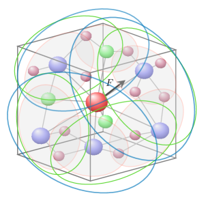
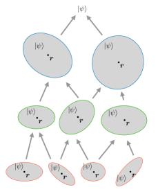
Figure 2. In a comp-net for learning atomic force fields, the output of each “part” $\mathcal{P}_{i}$ is $(\mbox{\boldmath$r$}_{i},\psi_{i})$, where $\mbox{\boldmath$r$}_{i}$ is the position vector of the corresponding physical subsystem, and $\psi_{i}$ is a vector describing its internal state.

Definition 3.

Let $\mathcal{S}$ be a physical system made up of $n$ particles $\xi_{1},\ldots,\xi_{n}$. An $\mathrm{SO}(3)$–covariant N–body neural network $\mathcal{N}$ for $\mathcal{S}$ is a composition scheme $\mathcal{D}$ in which

1. Each node $\mathfrak{n}_{j}$, which we will sometimes also call a gate, is associated with

   1. a physical sybsystem $\mathcal{P}_{j}$ of $\mathcal{S}$;

   2. a vector $\mbox{\boldmath$r$}_{j}\in\mathbb{R}^{3}$ describing the spatial poition of $\mathcal{P}_{j}$;

   3. a vector $\psi_{j}$ that that describes the internal state of $\mathcal{P}_{j}$ and is type $\mbox{\boldmath$\tau$}_{j}$ covariant to rotations.

2. If $\mathfrak{n}_{j}$ is a leaf node, then $\psi_{j}$ is determined by the corresponding particle $\xi_{j}$.

3. If $\mathfrak{n}_{j}$ is a non-leaf node and its children are $\mathfrak{n}_{\textrm{ch}_{1}},\ldots,\mathfrak{n}_{\textrm{ch}_{k}}$, then $\psi_{j}$ is computed as

   (5) $$\psi_{j}=\Phi_{j}(\widehat{r}_{\!\textrm{ch}_{1}},\ldots,\widehat{r}_{\textrm{ch}_{k}},\widehat{\mbox{\boldmath$r$}}_{\!\textrm{ch}_{1}},\ldots,\widehat{\mbox{\boldmath$r$}}_{\!\textrm{ch}_{k}},\psi_{\textrm{ch}_{1}}\ldots,\psi_{\textrm{ch}_{k}}),$$

   where $\widehat{\mbox{\boldmath$r$}}_{\!\textrm{ch}_{i}}=\mbox{\boldmath$r$}_{\!\textrm{ch}_{i}}-\mbox{\boldmath$r$}_{\!j}$ and $\widehat{r}_{i}=\left|\widehat{\mbox{\boldmath$r$}}_{i}\right|$. We call $\Phi_{j}$ the local aggregation rule.

4. $\mathcal{D}$ has a unique root $\mathfrak{n}_{r}$, and the output of the network, i.e., the learned state of the entire system is $\psi_{r}$. In the case of learning scalar valued functions, such as the atomic potential, $\psi_{r}$ is just a scalar.

Note that what is described in Definition 3 is a general architecture for learning the state of $N$–body physical systems with much wider applicability than just learning atomic potentials. The main technical challenge of the present paper is to define the $\Phi_{j}$ aggregation rules in such a way as to guarantee that each $\psi_{j}$ is $\mathrm{SO}(3)$–covariant. This is what is addressed in the following section.

4. Covariant aggregation rules

To define the aggregation function $\Phi$ to be used in $\mathrm{SO}(3)$–covariant comp-nets, all that we assume is that it is a polynomial in the relative positions $\widehat{\mbox{\boldmath$r$}}_{\textrm{ch}_{1}},\ldots,\widehat{\mbox{\boldmath$r$}}_{\textrm{ch}_{k}}$, the constituent state vectors $\psi_{\textrm{ch}_{1}},\ldots,\psi_{\textrm{ch}_{k}}$ and the inverse distances $1/\widehat{r}_{\textrm{ch}_{1}},\ldots 1/\widehat{r}_{\textrm{ch}_{k}}$. Specifically, we say that $\Phi$ is a $(P,Q,S)$–order aggregation function if each component of $\psi=\Phi(\widehat{r}_{\textrm{ch}_{1}},\ldots,\widehat{r}_{\textrm{ch}_{k}},\widehat{\mbox{\boldmath$r$}}_{\textrm{ch}_{1}},\ldots,\widehat{\mbox{\boldmath$r$}}_{\textrm{ch}_{k}},\psi_{\textrm{ch}_{1}}\ldots,\psi_{\textrm{ch}_{k}})$ is a polynomial of order at most $p$ in each component of $\mbox{\boldmath$r$}_{\textrm{ch}_{i}}$, a polynomial of at most $q$ in each component of $\psi_{\textrm{ch}_{i}}$, and a polynomial of order at most $s$ in each $1/(\widehat{r}_{\textrm{ch}_{i}})$. Any such $\Phi$ can be expressed as

(6) $$\Phi(\ldots)=\mathcal{L}\Bigl{(}\bigoplus_{\mathbf{p},\,\mathbf{q},\,\mathbf{s}}\mbox{\boldmath$r$}_{\textrm{ch}_{1}}^{\otimes p_{1}}\otimes\ldots\otimes\mbox{\boldmath$r$}_{\textrm{ch}_{k}}^{\otimes p_{k}}\otimes\psi_{\textrm{ch}_{1}}^{\otimes q_{1}}\otimes\ldots\otimes\psi_{\textrm{ch}_{k}}^{\otimes q_{k}}\cdot\widehat{r}_{\textrm{ch}_{1}}^{-s_{1}}\cdot\ldots\cdot\widehat{r}_{\textrm{ch}_{k}}^{-s_{k}}\Bigr{)},$$

where $\mathbf{p},\mathbf{q}$ and $\mathbf{s}$ are multi–indices of positive integers with $p_{i}\leq P$,  $q_{i}\leq Q$ and $s_{i}\leq S$, and $\mathcal{L}$ is a linear function. The tensor products appearing in (6) are formidably large object that in most cases would be impractical to compute explicitly. Rather, this equation is just meant to emphasize that any learnable parameters of the network must be implicit in the linear operator $\mathcal{L}$.

The more stringent requirements on $\mathcal{L}$ arise from the covariance criterion. The key to understanding these is the observation that for any sequence $\rho_{1},\ldots,\rho_{p}$ of (not necessarily irreducible) representations of a compact group $G$, their tensor product

$$\rho(R)=\rho_{1}(R)\otimes\rho_{2}(R)\otimes\ldots\otimes\rho_{p}(R)$$

is also a representation of $G$. Consequently, $\rho$ has a decomposition into irreps, similar to (2). As an immediate corollary, any product of $\mathrm{SO}(3)$ covariant vectors can be similarly decomposed. In particular, by applying the appropriate unitary matrix $C$, the sum of tensor products appearing in (6) can be decomposed into a sum of irreducible fragments in the form

$$\bigoplus_{\ell=0}^{L}\bigoplus_{m=1}^{\tau^{\prime}_{\ell}}\phi^{\ell}_{m}=C\biggl{(}\bigoplus_{\mathbf{p},\,\mathbf{q},\,\mathbf{s}}\mbox{\boldmath$r$}_{\textrm{ch}_{1}}^{\otimes p_{1}}\otimes\ldots\otimes\mbox{\boldmath$r$}_{\textrm{ch}_{k}}^{\otimes p_{k}}\otimes\psi_{\textrm{ch}_{1}}^{\otimes q_{1}}\otimes\ldots\otimes\psi_{\textrm{ch}_{k}}^{\otimes q_{k}}\cdot\widehat{r}_{\textrm{ch}_{1}}^{-s_{1}}\cdot\ldots\cdot\widehat{r}_{\textrm{ch}_{k}}^{-s_{k}}\biggr{)}.$$

To be explicit, we define

(7) $$\phi^{\ell}_{m}=T^{\ell}_{m}\biggl{(}\bigoplus_{\mathbf{p},\,\mathbf{q},\,\mathbf{s}}\mbox{\boldmath$r$}_{\textrm{ch}_{1}}^{\otimes p_{1}}\otimes\ldots\otimes\mbox{\boldmath$r$}_{\textrm{ch}_{k}}^{\otimes p_{k}}\otimes\psi_{\textrm{ch}_{1}}^{\otimes q_{1}}\otimes\ldots\otimes\psi_{\textrm{ch}_{k}}^{\otimes q_{k}}\cdot\widehat{r}_{\textrm{ch}_{1}}^{-s_{1}}\cdot\ldots\cdot\widehat{r}_{\textrm{ch}_{k}}^{-s_{k}}\biggr{)},$$

where $T^{0}_{1},\ldots,T^{0}_{\tau_{0}},T^{1}_{1},\ldots,T^{1}_{\tau_{2}},\ldots,T^{L}_{\tau_{L}}$ is an appropriate sequence of projection operators. The following proposition is a key result of our paper.

Proposition 1.

The output of the aggregation function (6) is a $\tau$–covariant vector if and only if $\mathcal{L}$ is of the form

(8) $$\mathcal{L}(\ldots)=\bigoplus_{\ell=0}^{L}\bigoplus_{m=1}^{\tau_{\ell}}\sum_{m^{\prime}=1}^{\tau^{\prime}_{\ell}}w^{\ell}_{m^{\prime},m}\,\phi^{\ell}_{m^{\prime}}.$$

Equivalently, collecting all $\phi^{\ell}_{m^{\prime}}$ fragments with the same $\ell$ into a matrix $\smash{\tilde{F}^{\ell}\in\mathbb{C}^{(2\ell+1)\times\tau^{\prime}_{\ell}}}$, all $(w^{\ell}_{m^{\prime},m})_{m^{\prime},m}$ weights into a matrix $\smash{W^{\ell}\in\mathbb{C}^{\tau^{\prime}_{\ell}\times\tau_{\ell}}}$, and reinterpreting the output of $\mathcal{L}$ as a collection of matrices rather than a single long vector,

(9) $$\mathcal{L}(\ldots)=\bigl{(}\tilde{F}^{0}W^{0},\tilde{F}^{1}W^{1},\ldots,\tilde{F}^{L}W^{L}\bigr{)}.$$

Proposition 1 tell us that $\mathcal{L}$ is only allowed to mix $\phi^{\ell}_{m}$ fragments with the same $\ell$, and that fragments can only be mixed in their entirety, rather than picking out their individual components. These are crucial consequences of equivariance. However, there are no further restrictions on the $(W^{\ell})_{\ell}$ mixing matrices.

In an $N$–body neural network the $W^{\ell}$ matrices are shared across (some subsets of) nodes, and it is these mixing (weight) matrices that the network learns from training data. The $\smash{\tilde{F}^{\ell}}$ matrices can be regarded as generalized matrix valued activations. Since each $W^{\ell}$ interacts with the $F^{\ell}$ matrices linearly, the network can be trained the usual way by backpropagating gradients of whatever loss function is applied to the output node $\mathfrak{n}_{r}$, whose activation is usually scalar valued.

It is important to note that $N$–body neural networks have no additional nonlinearity outside of $\Phi$, since that would break covariance. In contrast, in most existing neural network architectures, as explained in Section 2, each neuron first takes a linear combination of its inputs weighted by learned weights and then applies a fixed pointwise nonlinearity, $\sigma$. In our architecture the nonlinearity is hidden in the way that the $\phi^{\ell}_{m}$ fragments are computed, since a tensor product is a nonlinear function of its factors. On the other hand, mixing the resulting fragments with the $W^{\ell}$ weight matrices is a linear operation. Thus, in our case, the nonlinear part of the operation precedes the linear part.

The generic polynomial aggregation function (6) is too general to be used in a practical $N$–body network, and would be far too costly computationally. Instead, we propose using a few specific types of low order gates, such as those described below.

4.0.1. Zeroth order interaction gates

Zeroth order interaction gates aggregate the states of their children and combine them with their relative position vectors, but do not capture interactions between the children. A simple example of such a gate would be one where

(10) $$\Phi(\ldots)=\mathcal{L}\Bigl{(}\>\sum_{i=1}^{k}\hskip 1.00006pt(\psi_{\textrm{ch}_{i}}\otimes\widehat{\mbox{\boldmath$r$}}_{\textrm{ch}_{i}}),\;\sum_{i=1}^{k}\widehat{r}_{\textrm{ch}_{i}}^{-1}\hskip 1.00006pt(\psi_{\textrm{ch}_{i}}\otimes\widehat{\mbox{\boldmath$r$}}_{\textrm{ch}_{i}}),\;\sum_{i=1}^{k}\widehat{r}_{\textrm{ch}_{i}}^{-2}\hskip 1.00006pt(\psi_{\textrm{ch}_{i}}\otimes\widehat{\mbox{\boldmath$r$}}_{\textrm{ch}_{i}})\>\Bigr{)}.$$

Note that the summations in these formulae ensure that the output is invariant with respect to permuting the children and also reduce the generality of (6) because the direct sum is replaced by an explicit summation (this can also be interpreted as tying some of the mixing weights together in a particular way). Let $L$ be the largest $\ell$ for which $\tau_{\ell}\neq 0$ in the inputs. In the $L=0$ case each $\psi_{\textrm{ch}_{i}}$ state is a scalar quantity, such as electric charge. In the $L=1$ case it is a vector, such as the dipole moment. In the $L=2$ case it can encode the quadropole moment, and so on. A gate of the above form can learn how to combine such moments into a single (higher order) moment corresponding to the parent system.

It is instructive to see how many parameters a gate of this type has. Let us assume the simple case that each $\psi_{\textrm{ch}_{i}}$ is of type $\mbox{\boldmath$\tau$}=(1,1,\ldots,1)$ (up to $\ell=L$). The type of $\widehat{\mbox{\boldmath$r$}}_{\textrm{ch}_{i}}$ is $(0,1)$. According to the Clebsch–Gordan rules (see Section 4.1), the product of two such vectors is a vector of type $(1,3,2,\ldots,2,1)$ (of length $L+1$). Further assume that desired output type is again $\mbox{\boldmath$\tau$}=(1,1,\ldots,1)$ of length $L$. This means that the $\ell=L+1$ fragment does not even have to be computed, and the size of the weight matrices appearing in (9) are

$$W_{0}\in\mathbb{C}^{1\times 3}\qquad W_{1}\in\mathbb{C}^{1\times 9}\qquad W_{2}\in\mathbb{C}^{1\times 6}\qquad\ldots\qquad W_{L}\in\mathbb{C}^{1\times 6}.$$

The size of these matrices changes dramatically as we allow more “channels”. For example, if each of the input states are of type $\mbox{\boldmath$\tau$}=(c,c,\ldots,c)$, the type of $\psi_{\textrm{ch}_{i}}\otimes\widehat{\mbox{\boldmath$r$}}_{\textrm{ch}_{i}}$ becomes $(c,3c,2c,\ldots,2c,1c)$. Assuming again an output of type $\mbox{\boldmath$\tau$}=(c,c,\ldots,c)$, the weight matrices become

$$W_{0}\in\mathbb{C}^{c\times 3c}\qquad W_{1}\in\mathbb{C}^{c\times 9c}\qquad W_{2}\in\mathbb{C}^{c\times 6c}\qquad\ldots\qquad W_{L}\in\mathbb{C}^{c\times 6c}.$$

In many networks, however, the number of channels increases as we go higher in the network. Allowing the output type to be as rich as possible, without inducing linear redundancies, the output type becomes $(3c,9c,6c,\ldots,6c,3c)$, and

$$W_{0}\in\mathbb{C}^{3c\times 3c}\qquad W_{1}\in\mathbb{C}^{9c\times 9c}\qquad W_{2}\in\mathbb{C}^{6c\times 6c}\qquad\ldots\qquad W_{L}\in\mathbb{C}^{6c\times 6c}.$$

4.0.2. First order interaction gates

In first order interaction gates each of the children interact with each other, and the parent aggregates these pairwise interactions. A simple example would be computing the total energy of a collection of charged bodies, which might be done with a gate of the form

(11) $$\Phi(\ldots)=\mathcal{L}\Bigl{(}\>\sum_{i,j=1}^{k}\hskip 1.00006pt(\psi_{\textrm{ch}_{i}}\otimes\psi_{\textrm{ch}_{j}}\otimes\widehat{\mbox{\boldmath$r$}}_{\textrm{ch}_{i}}\otimes\widehat{\mbox{\boldmath$r$}}_{\textrm{ch}_{i}}),\;\sum_{i,j=1}^{k}\widehat{r}_{\textrm{ch}_{i}}^{-1}\widehat{r}_{\textrm{ch}_{j}}^{-1}\hskip 1.00006pt(\psi_{\textrm{ch}_{i}}\otimes\psi_{\textrm{ch}_{j}}\otimes\widehat{\mbox{\boldmath$r$}}_{\textrm{ch}_{i}}\otimes\widehat{\mbox{\boldmath$r$}}_{\textrm{ch}_{j}}),\;\\ \sum_{i,j=1}^{k}\widehat{r}_{\textrm{ch}_{i}}^{-2}\widehat{r}_{\textrm{ch}_{j}}^{-2}\hskip 1.00006pt(\psi_{\textrm{ch}_{i}}\otimes\psi_{\textrm{ch}_{j}}\otimes\widehat{\mbox{\boldmath$r$}}_{\textrm{ch}_{i}}\otimes\widehat{\mbox{\boldmath$r$}}_{\textrm{ch}_{j}}),\;\sum_{i,j=1}^{k}\widehat{r}_{\textrm{ch}_{i}}^{-3}\widehat{r}_{\textrm{ch}_{j}}^{-3}\hskip 1.00006pt(\psi_{\textrm{ch}_{i}}\otimes\psi_{\textrm{ch}_{j}}\otimes\widehat{\mbox{\boldmath$r$}}_{\textrm{ch}_{i}}\otimes\widehat{\mbox{\boldmath$r$}}_{\textrm{ch}_{j}})\;\Bigr{)}.$$

Generalizing (6) slightly, if we know that the interaction only depends on the relative positions of the child systems, we can also use

(12) $$\Phi(\ldots)=\mathcal{L}\Bigl{(}\>\sum_{i,j=1}^{k}\hskip 1.00006pt(\psi_{\textrm{ch}_{i}}\otimes\psi_{\textrm{ch}_{j}}\otimes\widehat{\mbox{\boldmath$r$}}_{\textrm{ch}_{i},\textrm{ch}_{j}}),\;\sum_{i,j=1}^{k}\widehat{r}_{\textrm{ch}_{i},\textrm{ch}_{j}}^{-1}\hskip 1.00006pt(\psi_{\textrm{ch}_{i}}\otimes\psi_{\textrm{ch}_{j}}\otimes\widehat{\mbox{\boldmath$r$}}_{\textrm{ch}_{i},\textrm{ch}_{j}}),\;\\ \sum_{i,j=1}^{k}\widehat{r}_{\textrm{ch}_{i},\textrm{ch}_{j}}^{-2}\hskip 1.00006pt(\psi_{\textrm{ch}_{i}}\otimes\psi_{\textrm{ch}_{j}}\otimes\widehat{\mbox{\boldmath$r$}}_{\textrm{ch}_{i},\textrm{ch}_{j}}),\;\sum_{i,j=1}^{k}\widehat{r}_{\textrm{ch}_{i},\textrm{ch}_{j}}^{-3}\hskip 1.00006pt(\psi_{\textrm{ch}_{i}}\otimes\psi_{\textrm{ch}_{j}}\otimes\widehat{\mbox{\boldmath$r$}}_{\textrm{ch}_{i},\textrm{ch}_{j}})\;\Bigr{)},$$

where $\widehat{\mbox{\boldmath$r$}}_{\textrm{ch}_{i},\textrm{ch}_{j}}=\widehat{\mbox{\boldmath$r$}}_{\textrm{ch}_{i}}\!-\widehat{\mbox{\boldmath$r$}}_{\textrm{ch}_{j}}$ and $\widehat{r}_{\textrm{ch}_{i},\textrm{ch}_{j}}=|\widehat{\mbox{\boldmath$r$}}_{\textrm{ch}_{i},\textrm{ch}_{j}}|$.

It is important to note that in the above electrostatics was used only as an example. There is no need to learn electrostatic interactions because they are perfectly described by classical physics. Rather, we envisage using the zeroth and first order interaction gates as constituents of a larger network for learning more complicated interactions with no simple closed form that nonetheless broadly follow similar scaling laws as classical interactions.

4.1. Clebsch–Gordan transforms

It remains to explain how the $T^{\ell}_{m}$ projection maps appearing in (7) are computed. This is critical because the nonlinearities in our network are the tensor products, and our architecture hinges on being able to reduce vectors into a direct sum of irreducibles again straight after the tensor product operation.

Fortunately, representation theory provides a clear prescription for how this operation is to be performed. For any compact group $G$, given two irreducible representations $\rho_{\ell_{1}}$ and $\rho_{\ell_{2}}$, the decomposition of $\rho_{\ell_{1}}\otimes\rho_{\ell_{2}}$ into a direct sum of irreducibles

(13) $$\rho_{\ell_{1}}(R)\otimes\rho_{\ell_{2}}(R)=C_{\ell_{1},\ell_{2}}^{\dagger}\Bigl{[}\>\bigoplus_{\ell}\bigoplus_{m=1}^{\kappa_{{{\tau}_{1},\mathbf{\tau}_{2}}}(\ell)~{}}\!\!\rho_{\ell}(R)\>\Bigr{]}\,C_{\ell_{1},\ell_{2}}$$

is called the Clebsch–Gordan transform. In the specific case of $\mathrm{SO}(3)$, the $\kappa$ multiplicities take on the very simple form (which we already used in Section 4.0.1)

$$\kappa_{\ell_{1},\ell_{2}}(\ell)=\begin{cases}~{}1&\text{if}~{}~{}\left|\ell_{1}-\ell_{2}\right|\leq\ell\leq\ell_{1}+\ell_{2}\\ ~{}0&\text{otherwise},\end{cases}$$

and the elements of the $C_{\ell_{1},\ell_{2}}$ matrices can also be computed relatively easily via closed form formulae.

We immediately see that (13) tells us how to reduce the product of covariant vectors into irreducible fragments. Assuming for example that $\psi_{1}$ is an irreducible $\rho_{\ell_{1}}$ vector and $\psi_{2}$ is an irreducible $\rho_{\ell_{2}}$ vector, $\psi_{1}\otimes\psi_{2}$ decomposes into irreducible fragments in the form

$$\psi_{1}\otimes\psi_{2}=\bigoplus_{\ell=\left|\ell_{1}-\ell_{2}\right|}^{\ell_{1}+\ell_{2}}\overline{\psi}{}^{\ell}\qquad\quad\text{where}\qquad\quad\overline{\psi}{}^{\ell}=C_{\ell_{1},\ell_{2},\ell}\,(\psi_{1}\otimes\psi_{2}),$$

and $C_{\ell_{1},\ell_{2},\ell}$ is the part of $C_{\ell_{1},\ell_{2}}$ matrix corresponding to the $\ell$’th “block”. Thus, in this case the operator $T^{\ell}_{1}$ just corresponds to mutiplying the tensor product by $C_{\ell_{1},\ell_{2},\ell}$. By linearity, the above relationship also extends to non-irreducible vectors. If $\psi_{1}$ is of type $\mbox{\boldmath$\tau$}_{1}$ and $\psi_{2}$ is of type $\mbox{\boldmath$\tau$}_{2}$, then

$$\psi_{1}\otimes\psi_{2}=\bigoplus_{\ell}\bigoplus_{m=1}^{\kappa_{\tau_{1},\tau_{2}}(\ell)}\overline{\psi}{}^{\ell}_{m}$$

where

$$\kappa_{\mbox{\boldmath$\tau$}_{1},\mbox{\boldmath$\tau$}_{2}}(\ell)=\sum_{\ell_{1}}\sum_{\ell_{2}}\;[\tau_{1}]_{\ell_{1}}\cdot[\tau_{2}]_{\ell_{2}}\>\cdot\mathbb{I}\left[\left|\ell_{1}-\ell_{2}\right|\leq\ell\leq\ell_{1}+\ell_{2}\right],$$

and $\mathbb{I}[\cdot]$ is the indicator function. Once again, the actual $\overline{\psi}{}^{\ell}_{m}$ fragments are computed by applying the appropriate $C_{\ell_{1},\ell_{2},\ell}$ matrix to the appropriate combination of irreducible fragments of $\psi_{1}$ and $\psi_{2}$. It is also clear that the by applying the Clebsch–Gordan decomposition recurisively, we can decompose a tensor product of any order, e.g.,

$$\psi_{1}\otimes\psi_{2}\otimes\psi_{3}\otimes\ldots\otimes\psi_{k}=((\psi_{1}\otimes\psi_{2})\otimes\psi_{3})\otimes\ldots\otimes\psi_{k}.$$

In an actual computation of such higher order products, however, a considerable amount of thought might have to go into optimizing the order of operations and reusing potential intermediate results to minimize computational cost.

5. Conclusions

There is considerable excitement in both the Machine Learning and the Physics/Chemistry communities about the potential of using neural networks to learn to the behavior and properties of complex physical systems. However, phyiscal systems have nontrivial invariance properties (in particular, invariance to translations, rotations and the exchange of identical elementary parts) that must be strictly respected.

In this paper we proposed a new type of generalized convolutional neural network architecture, $N$–body networks, which provides a flexible framework for modeling interacting systems of various types, while taking into account these invariances (symmetries). The specific motivation for developing $N$–body networks is to learn atomic potentials (force fields) for molecular dynamics simulations. However, we envisage that they will be used more broadly, for modeling a variety of systems. The closest to our work in certai ways are Moment Tensor Potientials (Shapeev, 2015), although that framework does not have learnable parameters.

$N$–body networks are distinguished from earlier neural network models for physical systems in that

1. The model is based on a hierarchical (but not necessarily strictly tree-like) decomposition of the system into subsystems at different levels, which is directly reflected in the structure of the neural network.

2. Each subsystem is identified with a “neuron” (or “gate”) $\mathfrak{n}_{i}$ in the network, and the output (activation) $\psi_{i}$ of the neuron becomes a representation of the subsystem’s internal state.

3. The $\psi_{i}$ states are tensorial objects with spatial character, in particular they are covariant with rotations in the sense that they transform under rotations according to specific irreducible representations of the rotation group. The gates are specially constructed to ensure that this covariance property is preserved throught the network.

4. Unlike most other neural network architectures, the nonlinearities in $N$–body networks are not pointwise operations, but are applied in “Fourier space”, i.e., directly to the irreducible parts of the state vector objects. This is only possible because (a) the nonlinearities arise as a consequence of taking tensor products of covariant objects (b) the tensor products are decomposed into irreducible parts by the Clebsch–Gordan transform.

We believe that the last of these ideas is particularly promising, because it suggests the possibility of constructing neural that operate entirely in Fourier space, and use tensor products combined with Clebsch–Gordan transforms to induce nonlinearities. This might have significance for a range of other applications, as well. Experiments are ongoing to validate our framework on real physical systems.

Acknowledgements

The author would like to thank Shubhendu Trivedi, Brandon Anderson, Hy Truong Son, Horace Pan, Gábor Csányi and Michele Ceriotti for their input to this work. Financial support for this work was provided in part by DARPA award number D16AP00112.

References

- Bartók et al. (2010) Albert P Bartók, Michael C Payne, Risi Kondor, and Gábor Csányi. Gaussian Approximation Potentials: the accuracy of quantum mechanics, without the electrons. Phys Rev Lett, 104(13):136403, 2010.
- Behler (2015) Jörg Behler. Constructing high-dimensional neural network potentials: A tutorial review. Int J Quantum Chem, 115(16):1032–1050, March 2015.
- Behler & Parrinello (2007) Jörg Behler and Michele Parrinello. Generalized neural-network representation of high-dimensional potential-energy surfaces. Phys Rev Lett, 98(14):146401, 2007.
- Brooks et al. (2009) B. R. Brooks, C. L. Brooks, A. D. Mackerell, L. Nilsson, R. J. Petrella, B. Roux, Y. Won, G. Archontis, C. Bartels, S. Boresch, and et al. CHARMM: the biomolecular simulation program. Journal of Computational Chemistry, 30(10):1545–1614, Jul 2009. ISSN 1096-987X.
- Brooks et al. (1983) Bernard R. Brooks, Robert E. Bruccoleri, Barry D. Olafson, David J. States, S. Swaminathan, and Martin Karplus. CHARMM: A program for macromolecular energy, minimization, and dynamics calculations. Journal of Computational Chemistry, 4(2):187–217, Jun 1983. ISSN 1096-987X.
- Bruna & Mallat (2013) Joan Bruna and Stephane Mallat. Invariant scattering convolutional networks. IEEE Transactions on Pattern Analysis and Machine Intelligence, 35:1872–1886, August 2013.
- Chmiela et al. (2016) Stefan Chmiela, Alexandre Tkatchenko, Huziel E. Sauceda, Igor Poltavsky, Kristof T. Schütt, and Klaus-Robert Müller. Machine Learning of Accurate Energy-Conserving Molecular Force Fields. (May):1–6, 2016. ISSN 2375-2548.
- Cohen & Welling (2016) Taco S. Cohen and Max Welling. Group equivariant convolutional networks. Proceedings of The 33rd International Conference on Machine Learning, 48:2990–2999, 2016.
- Cohen & Welling (2017) Taco S. Cohen and Max Welling. Steerable CNNs. In iclr, 2017.
- Cohen et al. (2018) Taco S. Cohen, Mario Geiger, Jonas Köhler, and Max Welling. Spherical CNNs. International Conference on Learning Representations, 2018.
- Defferrard et al. (2016) Michaël Defferrard, Xavier Bresson, and Pierre Vandergheynst. Convolutional neural networks on graphs with fast localized spectral filtering. In nips, 2016.
- Duvenaud et al. (2015) D. K. Duvenaud, D. Maclaurin, J. Iparraguirre, R. Bombarell, T. Hirzel, A. Aspuru-Guzik, and R. P. Adams. Convolutional networks on graphs for learning molecular fingerprints. In Advances in neural information processing systems, pp. 2224–2232, 2015.
- Gilmer et al. (2017) Justin Gilmer, Samuel S. Schoenholz, Patrick F. Riley, Oriol Vinyals, and George E. Dahl. Neural message passing for quantum chemistry. 2017.
- Hirn et al. (2017) M. Hirn, S. Mallat, and N. Poilvert. Wavelet scattering regression of quantum chemical energies. Multiscale Modeling & Simulation, 15(2):827–863, Jan 2017. ISSN 1540-3459.
- Hohenberg & Kohn (1964) P. Hohenberg and W. Kohn. Inhomogeneous electron gas. Phys. Rev., 136:864–871, 1964.
- Kearns et al. (2016) S. Kearns, K. McCloskey, M. Brendl, V. Pande, and P. Riley. Molecular graph convolutions: moving beyond fingerprints. Journal of Computer-Aided Molecular Design, 30:595–608, 2016.
- Kondor & Trivedi (2018) R. Kondor and S. Trivedi. On the generalization of equivariance and convolution in neural networks to the action of compact groups. 2018.
- Kondor et al. (2018) R. Kondor, Truong Son Hy, H. Pan, S. Trivedi, and B. M. Anderson. Covariant compositional networks for learning graphs. 2018.
- LeCun et al. (1998) Y. LeCun, Y. Bengio, and P. Haffner. Gradient-based learning applied to document recognition. Proceedings of the IEEE, pp. 2278–2324, 1998.
- Li et al. (2016) Yujia Li, Daniel Tarlow, Marc Brockschmidt, and Richard Zemel. Gated graph sequence neural networks. In iclr, 2016.
- Mallat (2012) S Mallat. Group Invariant Scattering. Technical report, 2012.
- Masci et al. (2015) Jonathan Masci, Davide Boscaini, Michael M. Bronstein, and Pierre Vandergheynst. Geodesic convolutional neural networks on riemannian manifolds. 2015.
- Monti et al. (2016) Federico Monti, Davide Boscaini, Jonathan Masci, Emanuele Rodola, Jan Svoboda, and Michael M. Bronstein. Geometric deep learning on graphs and manifolds using mixture model cnn. 2016.
- Niepert et al. (2016) M. Niepert, M. Ahmed, and K. Kutzkov. Learning convolutional neural networks for graphs. In Proceedings of the International Conference on Machine Learning, 2016.
- Schütt et al. (2017) Kristof T. Schütt, Farhad Arbabzadah, Stefan Chmiela, Klaus R. M uller, and Alexandre Tkatchenko. Quantum-chemical insights from deep tensor neural networks. Nature Communications, 8:13890, Jan 2017. ISSN 2041-1723.
- Serre (1977) Jean-Pierre Serre. Linear Representations of Finite Groups, volume 42 of Graduate Texts in Mathamatics. Springer-Verlag, 1977.
- Shapeev (2015) Alexander V Shapeev. Moment Tensor Potentials: a class of systematically improvable interatomic potentials. arXiv, December 2015.
- Zhang et al. (2017) Linfeng Zhang, Jiequn Han, Han Wang, Roberto Car, and Weinan E. Deep Potential Molecular Dynamics: a scalable model with the accuracy of quantum mechanics. arXiv:1707.09571 [physics], July 2017. arXiv: 1707.09571.