A Comparative Study of Pairwise Learning Methods based on Kernel Ridge Regression

Abstract

Many machine learning problems can be formulated as predicting labels for a pair of objects. Problems of that kind are often referred to as pairwise learning, dyadic prediction or network inference problems. During the last decade kernel methods have played a dominant role in pairwise learning. They still obtain a state-of-the-art predictive performance, but a theoretical analysis of their behavior has been underexplored in the machine learning literature.

In this work we review and unify existing kernel-based algorithms that are commonly used in different pairwise learning settings, ranging from matrix filtering to zero-shot learning. To this end, we focus on closed-form efficient instantiations of Kronecker kernel ridge regression. We show that independent task kernel ridge regression, two-step kernel ridge regression and a linear matrix filter arise naturally as a special case of Kronecker kernel ridge regression, implying that all these methods implicitly minimize a squared loss. In addition, we analyze universality, consistency and spectral filtering properties. Our theoretical results provide valuable insights in assessing the advantages and limitations of existing pairwise learning methods.

1 Introduction to pairwise learning

1.1 Settings in pairwise learning

Many real-world machine learning problems can naturally be represented as pairwise learning or dyadic prediction problems. In contrast to more traditional learning settings, the goal here consists of making predictions for pairs of objects $u\in\mathcal{U}$ and $v\in\mathcal{V}$, as elements of two universes $\mathcal{U}$ and $\mathcal{V}$. Such an ordered pair $(u,v)$ is often referred to as a dyad, and both elements in the dyad are usually equipped with a feature representation. In contrast to many statistical settings, these dyads are not independently and identically distributed, as the same objects tend to appear many times as part of different pairs.

Applications of pairwise learning often arise in the life sciences, such as predicting various types of interactions in all sorts of biological networks (e.g. drug-target networks, gene regulatory networks and species interaction networks). Similarly, pairwise learning methods are also used to extract novel relationships in social networks, such as author-citation networks. Other popular applications include recommender systems (predicting interactions between users and items) and information retrieval (predicting interactions between search queries and search results).

Formally speaking, in pairwise learning one attempts to learn a function of the form $f(u,v)$, i.e. a function to predict properties of two objects. Such functions are fitted using a set of $n$ labeled examples: the training set $S=\{(u_{h},v_{h},y_{h})\mid h=1,\ldots,n\}$. Further on, $U=\{u_{i}\mid i=1,\dots,m\}$ and $V=\{v_{j}\mid j=1,\ldots,q\}$ will denote the sets of distinct objects of both types, later refered to as instances and tasks, respectively, in the training set with $m=\arrowvert U\arrowvert$ and $q=\arrowvert V\arrowvert$.

Pairwise learning holds strong connections with many other machine learning settings. Especially a link with multi-task learning can be advocated, by calling the first object of a dyad an ‘instance’ and the second object a ‘task’. The underlying idea for making the distinction between instances and tasks is that the feature description of the instances is often considered as more informative, while the feature description of the tasks is mainly used to steer learning in the right direction. Albeit less common in traditional multi-task learning formulations, feature representations for tasks play a crucial role in recent paradigms such as zero-shot learning – see e.g. Palatucci et al., (2009); Lampert et al., (2014).

The connection between pairwise learning and multi-task learning allows one to distinguish different prediction settings that are crucial in the context of the paper. Formally, four settings for predicting the label of the dyad $(u,v)$ can be distinguished in pairwise learning, based on whether testing objects are in-sample (appear in the training data) or out-of-sample (do not appear in the training data):

• Setting A: Both $u$ and $v$ are observed during training, as parts of different dyads, but the label of the dyad $(u,v)$ must be predicted;

• Setting B: Only $v$ is known during training, while $u$ is not observed in any training dyad, and the label of the dyad $(u,v)$ must be predicted;

• Setting C: Only $u$ is known during training, while $v$ is not observed in any training dyad, and the label of the dyad $(u,v)$ must be predicted;

• Setting D: Neither $u$ nor $v$ occur in any training dyad, and the label of the dyad $(u,v)$ must be predicted.

Figure 1 visualizes data of the four settings graphically in four matrix representations. Setting A resembles a matrix completion or matrix filtering scenario, as typically encountered in collaborative filtering problems. In principle, feature representations are not needed if the structure of the matrix is exploited to generate predictions, but additional information might be helpful. Setting B resembles a classical multi-task learning scenario, where the columns represent instances and the rows tasks. For a predefined set of tasks, one aims for predicting the labels of novel instances. Setting C then considers the converse setting, where the instances are all known during training and some tasks are unobserved. This setting is in essence identical to Setting B, if one interchanges the notions of task and instance. Setting D is the most difficult prediction setting of all four. In the multi-task learning literature, this setting is known as zero-shot learning, as one aims for predicting the labels of tasks with zero training data.

In pairwise learning, it is extremely important to distinguish these four prediction scenarios. Without bearing them in mind, one might select the wrong model for the given scenario or obtain an under- or overestimation of the generalization error. For example, a pairwise recommender system that can generalize well to new users might perform poorly for new items. In a large-scale meta-study about biological network identification, it was found that these concepts are vital to correctly evaluate pairwise learning models (Park and Marcotte,, 2012). Certain properties of different models discussed in this work only hold for certain settings.

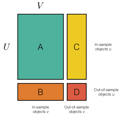
Figure 1: The different prediction settings in pairwise learning, depending on whether objects in a dyad occurred in the training set or not. Those four settings are further in this article always referred to as Setting A, B, C and D, respectively.

1.2 Kernel methods for pairwise learning with complete datasets

During the last decade various types of methods for pairwise learning have been proposed in the literature. Kernel methods in particular have been extensively used – see e.g. Vert and Yamanishi, (2005); Zaki et al., (2009); Huynh-Thu et al., (2010); van Laarhoven et al., 2011a ; Cao et al., (2012); Liu and Yang, (2015). Especially in bio-informatics applications they have been popular, because biological entities are often more easy to represent in terms of similarity scores than feature representations (Ben-Hur and Noble,, 2005; Shen et al.,, 2007; Vert et al.,, 2007).

In this work, we will focus on kernel methods for pairwise learning. We believe that kernel methods have a number of appealing properties:

• First, the existing methods that we analyze in this paper are general-purpose methods. They can be applied to a wide range of settings, including Settings  A, B, C and D, and a wide range of application domains. More recent methods might outperform kernel methods in specific situations, but they are usually not applicable to Settings A, B, C and D at the same time, or they are mainly developed for specific application domains with very specific types of datasets, e.g. computer vision and text mining datasets.

• Second, the methods that we analyze often form an essential building block of more recent (and more complicated) methods. This is, for example, the case for zero-shot learning methods in computer vision. It is therefore important to provide a theoretical analysis of older methods, in order to gain a better understanding of more recent methods that are often black-box engineering approaches. More details on this aspect will be given in a related work section at the end of this article.

• Third, the methods that we analyze in this paper are still clear winners for specific scenarios. One of those scenarios is cross-validation in pairwise learning, for which kernel methods outperform other methods substantially w.r.t. computational scalability. Furthermore, scalable and exact algorithms can be derived to learn a model online or when the dataset is not complete (see Definition 1 below). For more information on these aspects, we refer the reader to our complementary work (Stock et al., 2017a, ; Stock,, 2017; Stock et al.,, 2018).

These three reasons are the key motivations why it remains important to study kernel-based pairwise learning methods from a theoretical perspective. The key idea to extend kernel methods to pairwise learning is to construct so-called pairwise kernels, which measure the similarity between two dyads $(u,v)$ and $(\bar{u},\bar{v})$. Kernels of that kind can be used in tandem with any conventional kernelized learning algorithm, such as support vector machines, kernel ridge regression (KRR) and kernel Fisher discriminant analysis. In this article we will particularly focus on pairwise learning methods that are inspired by kernel ridge regression. Due to the algebraic properties of such methods, they are especially useful when analyzing so-called complete datasets in pairwise learning.

Definition 1 (Complete dataset)

A training set is called complete if it contains exactly one labeled example for every dyad $(u,v)\in U\times V$.

If the label matrix contains only a few missing labels, matrix imputation methods can be applied to render the matrix complete (Mazumder et al.,, 2010; Stekhoven and Bühlmann,, 2012; Zachariah and Sundin,, 2012). Complete datasets, however, occur frequently, for example in biological networks such as drug-protein interactions or species interactions. Here, screenings or field studies generate a set of observed interactions, while interactions that or not observed are either interactions not occurring or false negatives (Schrynemackers et al.,, 2013; Jordano,, 2016). In such cases, the positive instances are labeled as 1 whereas the negatives are labeled 0. Theoretical work by Elkan and Noto, (2008) has shown that models can still be learned from such datasets. Outside of biological network inference, complete datasets occur in recommender systems with implicit feedback, for example buying a book can be seen as a proxy for liking a book (Isinkaye et al.,, 2015). Setting A, i.e. re-estimating labels, is still relevant for such datasets if the labels are noisy or contain false positives or false negatives. A pairwise learning model can be used to detect and curate such errors.

For a complete training set we introduce a further notation for the matrix of labels $\mathbf{Y}\in\mathbb{R}^{m\times q}$, so that its rows are indexed by the objects in $U$ and the columns by the objects in $V$. Furthermore, we use $\mathbf{Y}_{i.}$, resp. $\mathbf{Y}_{.j}$, to denote the $i$-th row, resp. $j$-th column, of $\mathbf{Y}$. The vectorization of the matrix $\mathbf{Y}$ by stacking its columns in one long vector will be denoted $\mathbf{y}$.

1.3 Scope and objectives of this paper

The goal of this paper is to provide theoretical insights into the working of existing pairwise learning methods that are based on kernel ridge regression. To this end, we will focus on scenarios with complete training datasets, while analyzing the behavior for Settings A, B, C and D. More specifically, we intend to provide an in-depth discussion of the following four methods:

• Kronecker kernel ridge regression: adopting a least-squares formulation, this method is representative for many existing systems that are based on pairwise kernels.

• Two-step kernel ridge regression: this is a recent method that has some interesting properties such as simplicity and computational efficiency. The method has been independently proposed in Pahikkala et al., (2014) and Romera-Paredes and Torr, (2015). Also a variant of it exists, in which tree-based methods replace kernel ridge regression as base learners (Schrynemackers et al.,, 2015). In a statistical context, similar models have been developed for structural equation modelling (Bollen,, 1996; Bollen and Bauer,, 2004; Jung,, 2013).

• Linear matrix filtering: this is a recently-proposed method that is able to provide predictions in Setting A without the need for object features, similar to collaborative filtering methods. Though simple, this linear filter was found to perform very well to predict interactions in a variety of species-species and protein-ligand interaction datasets (Stock et al., 2017b, ; Stock,, 2017). On these datasets it outperforms standard matrix factorization methods, and it is very tolerant to a large number of false negatives in the label matrices.

• Independent-task kernel ridge regression: this method serves as a baseline and a building block for some of the other methods. This approach resembles the traditional kernel ridge regression method, applied to each task (i.e. each column of $\mathbf{Y}$) separately. When the method is applied to a single task, we will speak of single-task kernel ridge regression.

We will review these four models in Section 2. They can all be represented using two positive semidefinite kernel functions, on for each type of objects, i.e. $k:\mathcal{U}\times\mathcal{U}\rightarrow\mathbb{R}$ and $g:\mathcal{V}\times\mathcal{V}\rightarrow\mathbb{R}$. These capture the similarity between two objects of the same types. We will deal with prediction functions of the form:

$$f(u,v)=\sum_{i=1}^{m}\sum_{j=1}^{q}a_{ij}k(u,u_{i})g(v,v_{j})\,,$$ (1)

with $\mathbf{A}=[a_{ij}]\in\mathbb{R}^{m\times q}$ the dual parameters. Such a model can, for instance, be obtained by the pairwise Kronecker kernel in a kernel-based learning algorithm such as support vector machines – e.g. Vert et al., (2007); Brunner and Fischer, (2012). In this work, we will limit ourselves to models where the dual parameters can be written as a linear combination of the label matrix:

$$\textnormal{vec}(\mathbf{A})=\mathbf{B}\textnormal{vec}(\mathbf{Y})\,.$$ (2)

Here, $\mathbf{B}\in\mathbb{R}^{mq\times mq}$ is a matrix constructed based on the training objects $U$ and $V$, the kernel functions and the learning algorithm, but not the labels of the pairs. Similarly, the matrix containing the predictions $\mathbf{F}$ associated with the labels can be obtained by

$$\textnormal{vec}(\mathbf{F})=\mathbf{H}\textnormal{vec}(\mathbf{Y})\,,$$ (3)

where $\mathbf{H}\in\mathbb{R}^{mq\times mq}$ is the so-called hat matrix which maps observations to predictions (Hastie et al.,, 2001). Although $\mathbf{B}$ and $\mathbf{H}$ are huge matrices for problems of even modest sizes (i.e. if $|U|$ and $|V|$ are in the order of thousands, these matrices have a cardinality of millions), for several methods the parameters and predictions can be computed efficiently. More specifically, the learning algorithms discussed in this work scale with the number of objects rather than the number of labels.

The learning properties of the above four methods are theoretically analyzed in Section 3. In a first series of results, we establish equivalences via special kernels and algebraic operations. We discuss several links that are specific for Settings A, B, C or D. Figure 2 gives an overview of what the reader might expect to learn. In a second series of results we prove the universality of Kronecker product pairwise kernels, and we analyze the consistency of the algorithms that can be derived from such kernels. To this end, we provide a spectral interpretation of Kronecker and two-step kernel ridge regression. This will give further insights into the behavior of these methods.

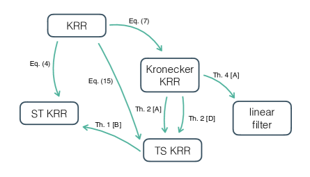
Figure 2: Overview of the different methods discussed in this work and their relation to one other: KRR = kernel ridge regression, ST KRR = single-task kernel ridge regression, TS KRR = two-step kernel ridge regression. The letters between brackets indicate the settings for which the theorem holds, as shown in Figure 1.

2 Pairwise learning with methods based on kernel ridge regression

In this section we formally review the four methods that were outlined in the introduction. We start by explaining a baseline multi-task learning formulation that will be needed to understand more complicated methods. We call this method independent-task kernel ridge regression, since it constructs independent models for the different tasks, i.e. the different columns of $\mathbf{Y}$. Subsequently, we elaborate on Kronecker kernel ridge regression as an instantiation of a method that employs pairwise kernels. In the last two paragraphs two-step kernel ridge regression and the linear matrix filter are reviewed. In what follows we adopt a multi-task learning formulation, in which the objects of $\mathcal{U}$ and $\mathcal{V}$ are referred to as instances and tasks, respectively.

2.1 Independent-task kernel ridge regression

Suppose that only features of objects of type $\mathcal{U}$ are available, but not of type $\mathcal{V}$. Since there is no information available on how the tasks are related, a separate model for each task is trained. Let $\mathbf{Y}_{.j}\in\mathbb{R}^{m}$ be the labels of task $v_{j}$ and $k(\cdot,\cdot)$ be a suitable kernel function what quantifies the similarity between the different instances. Since a separate and independent model is trained for each task, we will denote this setting as independent task (IT) kernel ridge regression. For each task $v_{j}$, one would like to learn a function of the form

$$f_{j}^{\mathrm{IT}}(u)=\sum_{i=1}^{m}a_{ij}^{\mathrm{IT}}k(u,u_{i})\,,$$

with $a_{ij}^{\mathrm{IT}}$ parameters that minimize a suitable objective function. In the case of KRR, this objective function is the squared loss with an $L_{2}$-complexity penalty. The parameters for the individual tasks using KRR can be found jointly by minimizing the following objective function (Wahba,, 1990; Bishop,, 2006):

$$J(\mathbf{A}^{\mathrm{IT}})=\textnormal{tr}[{(\mathbf{K}\mathbf{A}^{\mathrm{IT}}-\mathbf{Y})^{\top}(\mathbf{K}\mathbf{A}^{\mathrm{IT}}-\mathbf{Y})}]+\lambda_{u}\textnormal{tr}[{\mathbf{A}^{\mathrm{IT}}}^{\top}\mathbf{K}\mathbf{A}^{\mathrm{IT}}]\,,$$ (4)

with $\textnormal{tr}(\cdot)$ the trace, $\mathbf{A}^{\mathrm{IT}}=[a_{ij}^{\mathrm{IT}}]\in\mathbb{R}^{m\times q}$ and $\mathbf{K}\in\mathbb{R}^{m\times m}$ the Gram matrix associated with the kernel function $k(\cdot,\cdot)$ for the instances and $\lambda_{u}$ a regularization parameter. For simplicity, we assume the same regularization parameter $\lambda_{u}$ for each task $v$, though extensions to different penalties for different tasks are straightforward. This basic setting assumes no crosstalk between the tasks, as each model is fitted independently. The optimal coefficients that minimize Eq. (4) can be found by solving the following linear system:

$$\left(\mathbf{K}+\lambda_{u}\mathbb{I}\right)\mathbf{A}^{\mathrm{IT}}=\mathbf{Y}\,.$$ (5)

Using the singular value decomposition of the Gram matrix, this system can be solved for any value of $\lambda_{u}$ with a time complexity of $\mathcal{O}(m^{3}+m^{2}q)$.

2.2 Pairwise and Kronecker kernel ridge regression

Suppose one does have prior knowledge about which tasks are more similar, quantified by a kernel function $g(\cdot,\cdot)$ defined over the tasks. Several authors (see Álvarez et al., (2012); Baldassarre et al., (2012) and references therein) have extended KRR to incorporate task correlations via matrix-valued kernels. However, most of this literature concerns kernels for which the tasks are fixed at training time. An alternative approach, allowing for the generalization to new tasks more straightforwardly by means of such a task kernel, is to use a pairwise kernel $\Gamma\left(\left(u,v\right),\left(\bar{u},\bar{v}\right)\right)$. Pairwise kernels provide a prediction function of the type

$$f(u,v) =\sum_{h=1}^{n}\alpha_{h}\Gamma\left(\left(u,v\right),\left({u}_{h},{v}_{h}\right)\right)\,,$$ (6)

where $\boldsymbol{\alpha}=[\alpha_{h}]$ are parameters that minimize the same objective function as in (4):

$$J(\mathbf{\boldsymbol{\alpha}})=(\mathbf{\mathbf{\Gamma}}\mathbf{\boldsymbol{\alpha}}-\mathbf{y})^{\top}(\mathbf{\mathbf{\Gamma}}\mathbf{\boldsymbol{\alpha}}-\mathbf{y})+\lambda\mathbf{\boldsymbol{\alpha}}^{\top}\mathbf{\Gamma}\mathbf{\boldsymbol{\alpha}}\,,$$ (7)

with $\mathbf{\Gamma}$ the pairwise Gram matrix. The minimizer can also be found by solving a system of linear equations:

$$\left(\mathbf{\Gamma}+\lambda\mathbb{I}\right)\mathbf{\boldsymbol{\alpha}}=\mathbf{y}\,.$$ (8)

The most commonly used pairwise kernel is the Kronecker product pairwise kernel (Basilico and Hofmann, 2004a, ; Oyama and Manning,, 2004; Ben-Hur and Noble,, 2005; Park and Chu,, 2009; Hayashi et al.,, 2012; Bonilla et al.,, 2007; Pahikkala et al.,, 2013). This kernel is defined as

$$\Gamma^{\mathrm{KK}}\left(\left(u,v\right),\left(\bar{u},\bar{v}\right)\right)=k\left(u,\bar{u}\right)g\left(v,\bar{v}\right)\,,$$ (9)

a product of the data kernel $k(\cdot,\cdot)$ and the task kernel $g(\cdot,\cdot)$. Many other variations of pairwise kernels have been considered to incorporate prior knowledge on the nature of the relations (e.g. Vert et al., (2007); Pahikkala et al., (2010); Waegeman et al., (2012); Pahikkala et al., (2013)) or for more efficient calculations in certain settings – e.g. Kashima et al., (2010).

Let $\mathbf{\mathbf{G}}\in\mathbb{R}^{q\times q}$ be the Gram matrix for the tasks. Then, for a complete training set, the Gram matrix for the instance-task pairs is the Kronecker product $\mathbf{\Gamma}=\mathbf{\mathbf{G}}\otimes\mathbf{\mathbf{K}}$. Often it is infeasible to use this kernel directly due to its large size. The prediction function (6) can be written as

$$f^{\mathrm{KK}}(u,v)=\sum_{i=1}^{m}\sum_{j=1}^{q}a_{ij}^{\mathrm{KK}}k(u,u_{i})g(v,v_{j})\,.$$ (10)

The matrix $\mathbf{F}$ containing the predictions for the training data using a pairwise kernel can be obtained by a linear transformation of the training labels:

$$\textnormal{vec}(\mathbf{F}) =\mathbf{\Gamma}\textnormal{vec}(\mathbf{A}^{\mathrm{KK}})$$ (11)

$$=\mathbf{\Gamma}\left(\mathbf{\Gamma}+\lambda\mathbb{I}\right)^{-1}\textnormal{vec}(\mathbf{Y})$$ (12)

$$=\mathbf{H}^{\Gamma}\textnormal{vec}(\mathbf{Y})\,.$$ (13)

As a special case of Kronecker KRR, we also retrieve ordinary Kronecker kernel least-squares (OKKLS), when the objective function of Eq. (7) has no regularization term (i.e. $\lambda=0$).

Several authors have pointed out that, while the size of the system in Eq. (8) is considerably large, its solutions for the Kronecker product kernel can be found efficiently via tensor algebraic optimization (Van Loan,, 2000; Martin and Van Loan,, 2006; Kashima et al.,, 2009; Raymond and Kashima,, 2010; Pahikkala et al.,, 2013; Álvarez et al.,, 2012). This is because the eigenvalue decomposition of a Kronecker product of two matrices can easily be computed from the eigenvalue decomposition of the individual matrices. The time complexity scales roughly with $\mathcal{O}(m^{3}+q^{3})$, which is required for computing the singular value decomposition of $\mathbf{K}$ and $\mathbf{G}$ (see Property 2 in the appendix), but the complexities can be scaled down even further by using sparse kernel matrix approximation (Mahoney,, 2011; Gittens and Mahoney,, 2013).

However, these computational short-cuts only concern the case in which the training set is complete. If some of the instance-task pairs in the training set are missing or if there are several occurrences of certain pairs, one has to resort, for example, to gradient-descent-based training approaches (Park and Chu,, 2009; Pahikkala et al.,, 2013; Kashima et al.,, 2009; Airola and Pahikkala,, 2017). While the training can be accelerated via tensor algebraic optimization, such techniques still remain considerably slower than the approach based on eigenvalue decomposition.

2.3 Two-step kernel ridge regression

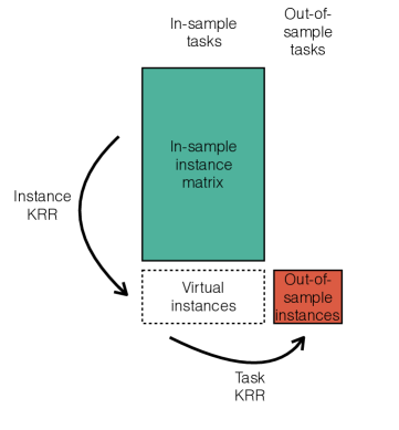
Figure 3: Principle of two-step KRR. In a first step, a virtual prediction is made for the out-of-sample tasks for new instances using a first KRR model. A second KRR model is trained using these data and this model is used to make predictions for new tasks.

Clearly, independent-task ridge regression can generalize to new instances, but not to new tasks as no dependence between these tasks is encoded in the model. Kronecker KRR, on the other hand, can be used for all four prediction settings depicted in Figure 1. But since our definition of ‘instances’ and ‘tasks’ is purely conventional, nothing is preventing us from building a model using the kernel function $g(\cdot,\cdot)$ to generalize to new tasks for the same instances. By combining two ordinary KRR s, one for generalizing to new instances and one that generalizes to new tasks, one can indirectly predict for new dyads.

More formally, suppose one wants to make a prediction for the dyad $(u,v)$. Let $\mathbf{k}\in\mathbb{R}^{m}$ denote the vector of instance kernel evaluations between the instances in the training set and an instance in the test set, i.e. $\mathbf{k}(u)=\left(k(u,u_{1}),\ldots,k(u,u_{m})\right)^{\top}$. Likewise, $\mathbf{g}\in\mathbb{R}^{q}$ represents the vector of task kernel evaluations between the target task and the auxiliary tasks, i.e. $\mathbf{g}(v)=\left(g(v,v_{1}),\ldots,g(v,v_{q})\right)^{\top}$. Based on the parameters found by solving Eq. (5), we can make a prediction for the new instance $u$ for all the auxiliary tasks:

$$\mathbf{f}_{V}(u)=\mathbf{k}^{\top}\left(\mathbf{K}+\lambda_{u}\mathbb{I}\right)^{-1}\mathbf{Y}\,,$$ (14)

with $\lambda_{u}$ the specific regularization parameter for the instances. This vector of predictions $\mathbf{f}_{V}(u)$ can be used as a set of labels in an intermediate step to train a second model for generalizing to new tasks for the same instance. Thus, using the task kernel and a regularization parameter for the tasks $\lambda_{v}$, one obtains:

$$f^{\mathrm{TS}}(u,v)=\mathbf{g}^{\top}\left(\mathbf{G}+\lambda_{v}\mathbb{I}\right)^{-1}\mathbf{f}_{V}(u)^{\top}\,,$$

or, by making use of Eq. (14), the prediction is given by

$$f^{\mathrm{TS}}(u,v) =\mathbf{k}^{\top}\left(\mathbf{K}+\lambda_{u}\mathbb{I}\right)^{-1}\mathbf{Y}\left(\mathbf{G}+\lambda_{v}\mathbb{I}\right)^{-1}\mathbf{g}$$ (15)

$$=\mathbf{k}^{\top}\mathbf{A}^{\mathrm{TS}}\mathbf{g}\,,$$ (16)

with $\mathbf{A}^{\mathrm{TS}}$ the dual parameters. The concept of two-step KRR is illustrated in Figure 3. Two-step KRR can be used for any of the prediction settings discussed in Section 1.1. Note that in practice there is no need to explicitly calculate $\mathbf{f}_{V}$, nor does it matter if in the first step one uses a model for new tasks and in the second step for instances, or the other way around.

This model can be cast in a similar form as the pairwise prediction function of Eq. (10) by making use of Property 1 in the appendix. Thus, for two-step KRR the parameters are given by

$$\mathbf{A}^{\mathrm{TS}} =\left(\mathbf{K}+\lambda_{u}\mathbb{I}\right)^{-1}\mathbf{Y}\left(\mathbf{G}+\lambda_{v}\mathbb{I}\right)^{-1}\,.$$ (17)

The time complexity for two-step KRR is the same as for Kronecker KRR: $\mathcal{O}(m^{3}+q^{3})$. The parameters can also be found by computing the eigenvalue decomposition of the two Gram matrices. Starting from these eigenvalue decompositions, it is possible to directly obtain the dual parameters for any values of the regularization hyperparameters $\lambda_{u}$ and $\lambda_{v}$. Because of its conceptual simplicity, it is quite straightforward to use two-step KRR for certain situations when the label matrix is not complete. The algebraic simplicity of two-step KRR can lead to some interesting algorithmic shortcuts for training and validating models. We refer to our other work for a theoretical and experimental overview (Stock,, 2017).

2.4 Linear filter for matrices

Single-task KRR uses a feature description only for the objects $u$, while Kronecker and two-step KRR incorporate feature descriptions of both objects $u$ and $v$. Is it possible to make predictions without any features at all? Obviously, this would only be possible for Setting A, where both objects are known during training. The structure of the label matrix $\mathbf{Y}$, e.g. being low rank, often contains enough information to successfully make predictions for this setting. In recommender systems, methods that do not take side features into account are often categorized as collaborative filtering methods (Su and Khoshgoftaar,, 2009).

In order to use our framework, we have to construct some feature description, in the form of a kernel function. An object $u$, resp. $v$, can be described by the observed labels of the dyads that contain the object. In the context of item recommendation, this seems reasonable: users are described by the ratings they have given to items and, likewise, items are described by users’ ratings. For example, Basilico and Hofman use a kernel based on the Pearson correlation of rating vectors of users to obtain a kernel description of users for collaborative filtering (Basilico and Hofmann, 2004b, ). In bioinformatics, van Laarhoven and colleagues predict drug-target interactions using so-called Gaussian interaction profile kernels, i.e. the classical radial basis kernel applied to the corresponding row or column of the label matrix (van Laarhoven et al., 2011b, ). There is nothing inherently wrong with using the labels to construct feature descriptions or kernels for the object. One should only be cautious when taking a holdout set for model selection or model evaluation; the omitted labels should also be removed from the feature description to prevent overfitting.

Kernels that take observed labels into account, such as the Gaussian interaction profile kernel, are in theory quite powerful. As they can be used to learn nonlinear associations, they lead to more expressive models than matrix factorization. The advantage of using these kernels compared to other collaborative filtering techniques such as matrix factorization, $k$-nearest neighbors or restricted Boltzmann machines, is that side features can elegantly be incorporated into the model. To this end, one only has to combine the collaborative and content-based kernel matrices, for example, by computing a weighted sum or element-wise multiplication.

Recently, a different method was proposed to make predictions without object features (Stock et al., 2017b, ). This method makes a prediction for a couple $(u_{i},v_{j})$ by aggregating the observed value, the row- and column average and the total average of the label matrix. By analogy with an image filter, this method was called a linear filter (LF) for matrices. The prediction matrix (Eq. (3)) is obtained as the following weighted average of averages:

$$\mathbf{F}_{ij}^{\text{LF}}=\alpha_{1}\mathbf{Y}_{ij}+\alpha_{2}\frac{1}{n}\sum_{k=1}^{n}\mathbf{Y}_{kj}+\alpha_{3}\frac{1}{m}\sum_{l=1}^{m}\mathbf{Y}_{il}+\alpha_{4}\frac{1}{nm}\sum_{k=1}^{n}\sum^{m}_{l=1}\mathbf{Y}_{kl}\,,$$ (18)

where $(\alpha_{1},\alpha_{2},\alpha_{3},\alpha_{4})\in[0,1]^{4}$. The first term is proportional to the label, while the last term is proportional to the average of all labels. The second (resp. third) term is proportional to the average label in the corresponding column (resp. row). The parameters $\alpha_{1},\alpha_{2},\alpha_{3}$ and $\alpha_{4}$ act as weighing coefficients.

As mentioned in the introduction, this linear filter can outcompete standard methods such as matrix factorization and it was observed to be particularly tolerant to a large number of false negatives in the label matrices. An attractive property of the linear filter is that it is possible to derive a computational short-cut for leave-one-pair-out (LOO) cross validation:

$$\mathbf{F}_{ij}^{\text{LOO}}=\frac{\mathbf{F}_{ij}-\left(\alpha_{1}+\frac{\alpha_{2}}{n}+\frac{\alpha_{3}}{m}+\frac{\alpha_{4}}{nm}\right)\mathbf{Y}_{ij}}{1-\left(\alpha_{1}+\frac{\alpha_{2}}{n}+\frac{\alpha_{3}}{m}+\frac{\alpha_{4}}{nm}\right)}\,.$$ (19)

This allows one to efficiently compute the prediction value $\mathbf{F}_{ij}^{\text{LOO}}$ using the label matrix except for the value $\mathbf{Y}_{ij}$.

In Section 3.2 we will show that this linear filter is a special instance of Kronecker KRR. This filter can hence be written in the form of Eq. (1) with the parameters obtained by solving a system of the form (2). In practice, however, one would always prefer to work directly using Eq. (18). The parameters $\alpha_{1},\alpha_{2},\alpha_{3}$ and $\alpha_{4}$ can be set by means of leave-one-pair-out cross-validation using Eq. (19).

3 Theoretical considerations

In Subsections 3.1 and 3.2 we show how the four methods of Section 2 are related via special kernels and algebraic equivalences. We establish several links that are specific for Setting A, B, C or D. Therefore, each result is formulated as a theorem that indicates the setting to which it applies in its header. In Subsection 3.3 the universality of the Kronecker product pairwise kernels is proven. This result provides a theoretical justification for the observation that Kronecker-based systems often obtain a very satisfactory performance in empirical studies. The universality is also used to prove the consistency of the methods that we analyze. This is done in Subsection 3.4 via a spectral interpretation. In addition, this interpretation also allows us to illustrate that two-step kernel ridge regression adopts a special decomposable filter.

3.1 Equivalence between two-step and other kernel ridge regression methods

The relation between two-step kernel ridge regression and independent-task ridge regression is given in the following theorem.

Theorem 3.1 (Setting B)

When the Gram matrix of the tasks $\mathbf{\mathbf{G}}$ is full rank and $\lambda_{v}$ is set to zero, independent-task KRR and two-step KRR return the same predictions for any given training task:

$$f^{\mathrm{IT}}_{j}(\cdot)\equiv f^{\mathrm{TS}}(\cdot,v_{j})\,.$$

Proof

The prediction for the independent-task KRR is given by:

$$f^{\mathrm{IT}}_{j}(u)=[\mathbf{k}^{\top}(\mathbf{K}+\lambda_{u}\mathbb{I})^{-1}\mathbf{Y}]_{j}\,.$$

For two-step KRR, it follows from Eq. (15) that

$$f^{\mathrm{TS}}_{j}(u) =[\mathbf{k}^{\top}(\mathbf{K}+\lambda_{u}\mathbb{I})^{-1}\mathbf{Y}\mathbf{G}^{-1}\mathbf{G}]_{j}$$

$$=[\mathbf{k}^{\top}(\mathbf{K}+\lambda_{u}\mathbb{I})^{-1}\mathbf{Y}]_{j}\,.$$

When $\mathbf{G}$ is singular, the $q$ outputs for the different tasks are projected on a lower-dimensional subspace by two-step KRR. This means that a dependence between the tasks is enforced, even when $\lambda_{v}=0$.

The connection between two-step and Kronecker KRR is established by the following results.

Theorem 3.2 (Setting A)

Consider the following pairwise kernel matrix:

$$\mathbf{\Xi} =\mathbf{G}\otimes\mathbf{K}\left(\lambda_{u}\lambda_{v}\mathbb{I}\otimes\mathbb{I}+\lambda_{v}\mathbb{I}\otimes\mathbf{K}+\lambda_{u}\mathbf{G}\otimes\mathbb{I}\right)^{-1}\,.$$

The predictions for the training data $\mathbf{F}$ using pairwise KRR (Eq. (12)) with the above pairwise kernel and regularization parameter $\lambda=1$ correspond to those obtained with two-step KRR using the kernel matrices $\mathbf{K}$, $\mathbf{G}$ with respective regularization parameters $\lambda_{u}$ and $\lambda_{v}$.

Proof

We will formulate the corresponding empirical risk minimization of Eq. (7) from the perspective of value regularization. Since Setting A is an imputation setting, we directly search for the optimal predicted label matrix $\mathbf{F}$, rather than the optimal parameter matrix. Starting from the objective function for Kronecker KRR, the predictions for the training data are obtained through minimizing the following variational function:

$$J(\mathbf{F}) =\textnormal{vec}(\mathbf{F}-\mathbf{Y})^{\top}\textnormal{vec}(\mathbf{F}-\mathbf{Y})+\textnormal{vec}(\mathbf{F})^{\top}\mathbf{\Xi}^{-1}\textnormal{vec}(\mathbf{F})$$ (20)

$$=\textnormal{vec}(\mathbf{F}-\mathbf{Y})^{\top}\textnormal{vec}(\mathbf{F}-\mathbf{Y})$$

$$\qquad+\textnormal{vec}(\mathbf{F})^{\top}\left(\mathbf{G}\otimes\mathbf{K}\left(\lambda_{u}\lambda_{v}\mathbb{I}\otimes\mathbb{I}+\lambda_{v}\mathbb{I}\otimes\mathbf{K}+\lambda_{u}\mathbf{G}\otimes\mathbb{I}\right)^{-1}\right)^{-1}\textnormal{vec}(\mathbf{F})$$

$$=\textnormal{vec}(\mathbf{F}-\mathbf{Y})^{\top}\textnormal{vec}(\mathbf{F}-\mathbf{Y})$$

$$\qquad+\textnormal{vec}(\mathbf{F})^{\top}\left(\mathbf{G}^{-1}\otimes\mathbf{K}^{-1}\left(\lambda_{u}\lambda_{v}\mathbb{I}\otimes\mathbb{I}+\lambda_{v}\mathbb{I}\otimes\mathbf{K}+\lambda_{u}\mathbf{G}\otimes\mathbb{I}\right)\right)\textnormal{vec}(\mathbf{F})$$

$$=\textnormal{vec}(\mathbf{F}-\mathbf{Y})^{\top}\textnormal{vec}(\mathbf{F}-\mathbf{Y})$$

$$\qquad+\textnormal{vec}(\mathbf{F})^{\top}\left(\lambda_{u}\lambda_{v}\mathbf{G}^{-1}\otimes\mathbf{K}^{-1}+\lambda_{u}\mathbb{I}\otimes\mathbf{K}^{-1}+\lambda_{v}\mathbf{G}^{-1}\otimes\mathbb{I}\right)\textnormal{vec}(\mathbf{F})$$

$$=\textnormal{tr}((\mathbf{F}-\mathbf{Y})^{\top}(\mathbf{F}-\mathbf{Y})+\lambda_{u}\lambda_{v}\mathbf{F}^{\top}\mathbf{K}^{-1}\mathbf{F}\mathbf{G}^{-1}$$

$$\qquad+\lambda_{u}\mathbf{F}^{\top}\mathbf{K}^{-1}\mathbf{F}+\lambda_{v}\mathbf{F}^{\top}\mathbf{F}\mathbf{G}^{-1})\,.$$

The derivative with respect to $\mathbf{F}$ is given by:

$$\frac{\partial J(\mathbf{F})}{\partial\mathbf{F}} =2(\mathbf{F}-\mathbf{Y}+\lambda_{u}\lambda_{v}\mathbf{K}^{-1}\mathbf{F}\mathbf{G}^{-1}+\lambda_{u}\mathbf{K}^{-1}\mathbf{F}+\lambda_{v}\mathbf{F}\mathbf{G}^{-1})$$

$$=2(\lambda_{u}\mathbf{K}^{-1}+\mathbb{I})\mathbf{F}+2(\lambda_{u}\mathbf{K}^{-1}+\mathbb{I})(\lambda_{v}\mathbf{F}\mathbf{G}^{-1})-2\mathbf{Y}$$

$$=2(\lambda_{u}\mathbf{K}^{-1}+\mathbb{I})\mathbf{F}(\lambda_{v}\mathbf{G}^{-1}+\mathbb{I})-2\mathbf{Y}\,.$$

Setting it to zero and solving with respect to $\mathbf{F}$ yields:

$$\mathbf{F} =(\lambda_{u}\mathbf{K}^{-1}+\mathbb{I})^{-1}\mathbf{Y}(\lambda_{v}\mathbf{G}^{-1}+\mathbb{I})^{-1}$$

$$=\mathbf{K}(\mathbf{K}+\lambda_{u}\mathbb{I})^{-1}\mathbf{Y}(\mathbf{G}+\lambda_{v}\mathbb{I})^{-1}\mathbf{G}\,.$$

Comparing with Eq. (17), we note that $\mathbf{F}=\mathbf{K}\mathbf{A}^{\mathrm{TS}}\mathbf{G}$, which proves the theorem.

Here, we have assumed that $\mathbf{K}$ and $\mathbf{G}$ are invertible. Note that the kernel $\mathbf{\Xi}$ can always be obtained as long as $\mathbf{K}$ and $\mathbf{G}$ are positive semi-definite. The relevance of the above theorem is that it formulates two-step KRR as an empirical risk minimization problem for Setting A (Eq. (20)). It is important to note that the pairwise kernel matrix $\mathbf{\Xi}$ only appears in the regularization term of this variational problem. The loss function is only dependent on the predicted values $\mathbf{F}$ and the label matrix $\mathbf{Y}$. Using two-step KRR for Setting A when dealing with incomplete data is thus well defined. The empirical risk minimization problem of Eq. (20) can be modified so that the squared loss only takes the observed dyads into account:

$$J^{\prime}(\mathbf{F})=\sum_{(u,v,y)\in S}(y-f(u,v)))^{2}+\textnormal{vec}(\mathbf{F})^{\top}\mathbf{\Xi}^{-1}\textnormal{vec}(\mathbf{F})\,,$$ (21)

with $S$ the training set of labeled dyads. In this case, one ends up with a transductive setting. This explains why Setting A is the most easy setting to predict for, as in transductive learning one only has to predict for a finite number of dyads known during training, in contrast to inductive learning where the model has to make predictions for any new dyad, a harder problem (Chapelle et al.,, 2006). See Rifkin and Lippert, (2007); Johnson and Zhang, (2008) for a more in-depth discussion.

Two-step and Kronecker KRR also coincide in an interesting way for Setting D (e.g. the special case in which there is no labeled data available for the target task). This, in turn, will allow us to show the consistency of two-step KRR via its universal approximation and spectral regularization properties. The theorem below shows the relation between two-step KRR and ordinary Kronecker KRR for Setting D.

Theorem 3.3 (Setting D)

Consider a setting with a complete training set. Let $f^{\mathrm{TS}}(\cdot,\cdot)$ be a model trained with two-step KRR and $f^{\mathrm{OKKLS}}(\cdot,\cdot)$ be a model trained with ordinary Kronecker kernel least-squares regression (OKKLS) using the following pairwise kernel function on $\mathcal{U}\times\mathcal{V}$:

$$\Upsilon\left(\left(u,v),(\bar{u},\bar{v}\right)\right)=\left(k\left(u,\bar{u}\right)+\lambda_{u}\delta\left(u,\bar{u}\right)\right)\left(g\left(v,\bar{v})+\lambda_{v}\delta\left(v,\bar{v}\right)\right)\right)$$ (22)

where $\delta$ is the delta kernel whose value is 1 if the arguments are equal and 0 otherwise. Then for making predictions for instances $u\in\mathcal{U}\setminus U$ and tasks $v\in\mathcal{V}\setminus V$ not seen in the training set, it holds that $f^{\mathrm{TS}}(u,v)=f^{\mathrm{OKKLS}}(u,v)$.

Proof

From Eq. (15) we have the following dual model for prediction:

$$f^{\mathrm{TS}}(u,v)=\sum_{i=1}^{m}\sum_{j=1}^{q}a_{ij}^{\mathrm{TS}}k(u,u_{i})g(v,v_{j})\,,$$

with $\mathbf{A}^{\mathrm{TS}}=[a_{ij}^{\mathrm{TS}}]$ the matrix of parameters. Similarly, the dual representation of the OKKLS (see Eq. (10)), using a parametrization $\mathbf{A}^{\mathrm{OKKLS}}=[a_{ij}^{\mathrm{OKKLS}}]$, is given by

$$f^{\mathrm{OKKLS}}(u,v) =\sum_{i=1}^{m}\sum_{j=1}^{q}a_{ij}^{\mathrm{OKKLS}}\Upsilon\left(\left(u,v),(u_{i},v_{j}\right)\right)$$

$$=\sum_{i=1}^{m}\sum_{j=1}^{q}a_{ij}^{\mathrm{OKKLS}}(k(u,{u}_{i})+\lambda_{u}\delta(u,{u}_{i}))(g(v,{v}_{j})$$

$$\qquad\qquad+\lambda_{v}\delta(v,{v}_{j})))$$

$$=\sum_{i=1}^{m}\sum_{j=1}^{q}a_{ij}^{\mathrm{OKKLS}}k(u,u_{i})g(v,v_{j})\,.$$

In the last step we used the fact that $u\neq u_{i}$ and $v\neq v_{j}$ to drop the delta kernels. Hence, we need to show that $\mathbf{A}^{\mathrm{TS}}=\mathbf{A}^{\mathrm{OKKLS}}$.

By Eq. (17) and denoting $\widetilde{\mathbf{G}}=\left(\mathbf{G}+\lambda\mathbb{I}\right)^{-1}$ and $\widetilde{\mathbf{K}}=\left(\mathbf{K}+\lambda\mathbb{I}\right)^{-1}$, we observe that the model parameters $\mathbf{A}^{\mathrm{TS}}$ of the two-step model can also be obtained in the following closed form:

$$\mathbf{A}^{\mathrm{TS}} =\widetilde{\mathbf{K}}\mathbf{Y}\widetilde{\mathbf{G}}\,.$$ (23)

The kernel matrix of $\Upsilon$ for Setting D can be expressed as: $\mathbf{\Upsilon}=\left(\mathbf{G}+\lambda_{v}\mathbb{I}\right)\otimes\left(\mathbf{K}+\lambda_{u}\mathbb{I}\right)\,.$ The OKKLS problem with kernel $\Upsilon$ being

$$\textnormal{vec}(\mathbf{A}^{\mathrm{OKKLS}})=\\ \qquad\underset{\mathbf{A}\in\mathbb{R}^{m\times q}}{\operatorname{arg}\,\operatorname{min}}\;\left(\textnormal{vec}(\mathbf{Y})-\mathbf{\Upsilon}\textnormal{vec}(\mathbf{A})\right)^{\top}\left(\textnormal{vec}(\mathbf{Y})-\mathbf{\Upsilon}\textnormal{vec}(\mathbf{A})\right)\,,$$

its minimizer can be expressed as

$$\textnormal{vec}(\mathbf{A}^{\mathrm{OKKLS}}) =\mathbf{\Upsilon}^{-1}\textnormal{vec}(\mathbf{Y})=\left(\left(\mathbf{G}+\lambda_{v}\mathbb{I}\right)^{-1}\otimes\left(\mathbf{K}+\lambda_{u}\mathbb{I}\right)^{-1}\right)\textnormal{vec}(\mathbf{Y})$$

$$=\textnormal{vec}\left(\left(\mathbf{K}+\lambda_{u}\mathbb{I}\right)^{-1}\mathbf{Y}\left(\mathbf{G}+\lambda_{v}\mathbb{I}\right)^{-1}\right)=\textnormal{vec}\left(\widetilde{\mathbf{K}}\mathbf{Y}\widetilde{\mathbf{G}}\right)\,.$$ (24)

Here we again make use of Property 1 in the appendix. From Eq. (3.1) it then follows that $\mathbf{A}^{\mathrm{TS}}=\mathbf{A}^{\mathrm{OKKLS}}$, which proves the theorem.

3.2 Smoother kernels lead to the linear filter

Here, we will show that using Kronecker KRR in tandem with certain kernels results in the linear filter of Section 2.4. When no good features of the objects are available, we propose to use different kernels, ‘agnostic’ of the true objects:

$$k^{\text{SM}}\text{(}u,\bar{u}) =1+\theta_{u}\delta(u,\bar{u})$$

$$g^{\text{SM}}(v,\bar{v}) =1+\theta_{v}\delta(v,\bar{u})\,,$$

or, equivalently, as Gram matrices:

$$\mathbf{K}=\mathbb{J}_{m\times m}+\theta_{u}\mathbb{I}_{m}\qquad\text{ and }\qquad\mathbf{G}=\mathbb{J}_{q\times q}+\theta_{v}\mathbb{I}_{q}\,.$$ (25)

Here, $\theta_{u}$ and $\theta_{v}$ are two hyperparameters of the kernels, $\mathbb{J}_{m\times m}$ is an ${m\times m}$ matrix filled with ones and $\mathbb{J}_{q\times q}$ is an ${q\times q}$ matrix filled with ones. We will call these kernels smoother kernels for reasons that will become clear. The rationale behind these kernels is quite simple: a kernel that is the identity matrix would imply that all objects are unique and independent; there is no similarity between them. Using the all-ones matrix on the other hand encodes all objects being exactly the same; no distinction between two objects can be made. Hence, the kernels of (25) represent a trade-off between all objects being similar (first part) and all objects being unique (second part). This is controlled by the hyperparameters $\theta_{u}$ and $\theta_{v}$.

Using these kernels in the Kronecker-based models has an interesting interpretation: the predictions can be written as a weighted sum of averages.

Theorem 3.4 (Smoother kernels)

Predictions using Kronecker KRR for Setting A using the Gram matrices (25) are of the form:

$$f(u_{i},v_{j})=\alpha_{1}\mathbf{Y}_{ij}+\alpha_{2}\frac{1}{q}\sum_{l=1}^{q}\mathbf{Y}_{il}+\alpha_{3}\frac{1}{m}\sum_{k=1}^{m}\mathbf{Y}_{kj}+\alpha_{4}\frac{1}{mq}\sum^{m}_{k=1}\sum^{q}_{l=1}\mathbf{Y}_{kl}\,,$$

with $(\alpha_{1},\alpha_{2},\alpha_{3},\alpha_{4})\in\mathbb{R}^{4}$.

Proof

For Setting A, the hat matrix of Eq. (3) transforms the label matrix in the prediction matrix. The hat matrix $\mathbf{H}^{\text{SM}}$ for Kronecker KRR using these smoother kernels can be obtained by applying Eq. (13):

$$\mathbf{H}^{\text{SM}}=a_{1}\mathbb{I}_{q}\otimes\mathbb{I}_{m}+a_{2}\mathbb{J}_{q}\otimes\mathbb{I}_{m}+a_{3}\mathbb{I}_{q}\otimes\mathbb{J}_{m}+a_{4}\mathbb{J}_{q}\otimes\mathbb{J}_{m}\,.$$ (26)

This can easily be seen because the pairwise Gram matrix will be of the form (26) and Properties 3 and 4 state that multiplying or inverting matrices of the form (26) results in a matrix of the same form. From these properties, it follows that the hat matrix will also be of this form.

The prediction for dyad $(u_{i},v_{j})$ is given by $[\mathbf{H}^{\text{SM}}\textnormal{vec}(\mathbf{Y})]_{jq+i}$. Using the relation between the Kronecker product and the vectorization operation, each term of (26) can be rewritten using Property 1 as follows

$$a_{1}[(\mathbb{I}_{q}\otimes\mathbb{I}_{m})\textnormal{vec}(\mathbf{Y})]_{jm+i}=a_{1}[\mathbb{I}_{m}\mathbf{Y}\mathbb{I}_{q}]_{ij} =a_{1}\mathbf{Y}_{ij}$$

$$a_{2}[(\mathbb{J}_{q\times q}\otimes\mathbb{I}_{m})\textnormal{vec}(\mathbf{Y})]_{jm+i}=a_{2}[\mathbb{I}_{m}\mathbf{Y}\mathbb{J}_{q\times q}]_{ij} =a_{2}\sum_{l=1}^{q}\mathbf{Y}_{il}$$

$$a_{3}[(\mathbb{I}_{q}\otimes\mathbb{J}_{m\times m})\textnormal{vec}(\mathbf{Y})]_{jm+i}=a_{3}[\mathbb{J}_{m\times m}\mathbf{Y}\mathbb{I}_{q}]_{ij} =a_{3}\sum_{k=1}^{m}\mathbf{Y}_{kj}$$

$$a_{4}[(\mathbb{J}_{q\times q}\otimes\mathbb{J}_{m\times m})\textnormal{vec}(\mathbf{Y})]_{jm+i}=a_{4}[\mathbb{J}_{m\times m}\mathbf{Y}\mathbb{J}_{q\times q}]_{ij} =a_{4}\sum_{l=1}^{q}\sum_{k=1}^{m}\mathbf{Y}_{kl}\,,$$

which proves the theorem.

The smoother kernel is thus quite restrictive in the type of models that can be learned. It can only exploit the fact that some rows or columns have a larger average value (e.g. in item recommendation, some items in collaborative filtering have a high average rating, independent for the user). Nevertheless, it can lead to good baseline predictions for Setting A and is particularly useful for small datasets with no side-features, such as species interaction networks.

3.3 Universality of the Kronecker product pairwise kernel

Here we consider the universal approximation properties of Kronecker KRR and, by Theorems 3.2 and 3.3, of two-step KRR. This is a necessary step in showing the consistency of the latter method. First, recall the concept of universal kernel functions.

Definition 2

(Steinwart,, 2002) A continuous kernel $k(\cdot,\cdot)$ on a compact metric space $\mathcal{X}$ (i.e. $\mathcal{X}$ is closed and bounded) is called universal if the reproducing kernel Hilbert space (RKHS) induced by $k(\cdot,\cdot)$ is dense in $C(\mathcal{X})$, where $C(\mathcal{X})$ is the space of all continuous functions $f:\mathcal{X}\rightarrow\mathbb{R}$.

The universality property indicates that the hypothesis space induced by a universal kernel can approximate any continuous function on the input space $\mathcal{X}$ to be learned arbitrarily well, given that the available set of training data is large and representative enough, and the learning algorithm can efficiently find this approximation from the hypothesis space (Steinwart,, 2002). In other words, the learning algorithm is consistent in the sense that, informally put, the hypothesis learned by it gets closer to the function to be learned while the size of the training set gets larger. The consistency properties of two-step KRR are considered in more detail in Subsection 3.4.

Next, we consider the universality of the Kronecker product pairwise kernel. The following result is a straightforward modification of some of the existing results in the literature (e.g. Waegeman et al., (2012)), but it is presented here for self-containedness. This theorem is mainly related to Setting D, while it also covers the other settings as special cases.

Theorem 3.5

The kernel $\Gamma^{\mathrm{KK}}((\cdot,\cdot),(\cdot,\cdot))$ on $\mathcal{U}\times\mathcal{V}$ defined in Eq. (9) is universal if the instance kernel $k(\cdot,\cdot)$ on $\mathcal{U}$ and the task kernel $g(\cdot,\cdot)$ on $\mathcal{V}$ are both universal.

Proof

Let us define

$$\begin{array}[]{l}\mathcal{A}\otimes\mathcal{B}=\left\{t\mid t(u,v)=a(u)b(v),a\in\mathcal{A},b\in\mathcal{B}\right\}\end{array}$$ (27)

for compact metric spaces $\mathcal{U}$ and $\mathcal{V}$ and sets of functions $\mathcal{A}\subset C(\mathcal{U})$ and $\mathcal{B}\subset C(\mathcal{V})$. We observe that the RKHS of the kernel $\Gamma$ can be written as $\mathcal{H}(k)\otimes\mathcal{H}(g)$, where $\mathcal{H}(k)$ and $\mathcal{H}(g)$ are the RKHS of the kernels $k(\cdot,\cdot)$ and $g(\cdot,\cdot)$, respectively.

Let $\epsilon>0$ and let $t\in C(\mathcal{U})\otimes C(\mathcal{V})$ be an arbitrary function that, according to Eq. (27), can be written as $t(u,v)=a(u)b(v)$, where $a\in C(\mathcal{U})$ and $b\in C(\mathcal{V})$. By definition of the universality property, $\mathcal{H}(k)$ and $\mathcal{H}(g)$ are dense in $C(\mathcal{U})$ and $C(\mathcal{V})$, respectively. Therefore, there exist functions $\bar{a}\in\mathcal{H}(k)$ and $\bar{b}\in\mathcal{H}(g)$ such that

$$\max_{u\in\mathcal{U}}\left\arrowvert\bar{a}(u)-a(u)\right\arrowvert\leq\bar{\epsilon},\qquad\max_{v\in\mathcal{V}}\left\arrowvert\bar{b}(v)-b(v)\right\arrowvert\leq\bar{\epsilon}\,,$$

where $\bar{\epsilon}$ is a constant for which it holds that

$$\max_{u\in\mathcal{U},v\in\mathcal{V}}\left\{\left\arrowvert\bar{\epsilon}\,a(u)\right\arrowvert+\left\arrowvert\bar{\epsilon}\,b(v)\right\arrowvert+\bar{\epsilon}^{2}\right\}\leq\epsilon\,.$$

Note that, according to the extreme value theorem, the maximum exists due to the compactness of $\mathcal{U}$ and $\mathcal{V}$ and the continuity of the functions $a(\cdot)$ and $b(\cdot)$. Now we have

$$\begin{array}[]{l}\displaystyle\max_{u\in\mathcal{U},v\in\mathcal{V}}\left\arrowvert t(u,v)-\bar{a}(u)\bar{b}(v)\right\arrowvert\\ \displaystyle\leq\max_{u\in\mathcal{U},v\in\mathcal{V}}\left\arrowvert t(u,v)-a(u)b(v)\right\arrowvert+\left\arrowvert\bar{\epsilon}\,a(u)\right\arrowvert+\left\arrowvert\bar{\epsilon}\,b(v)\right\arrowvert+\bar{\epsilon}^{2}\\ \displaystyle=\max_{u\in\mathcal{U},v\in\mathcal{V}}\left\arrowvert\bar{\epsilon}\,a(u)\right\arrowvert+\left\arrowvert\bar{\epsilon}\,b(v)\right\arrowvert+\bar{\epsilon}^{2}\leq\epsilon,\end{array}$$

which confirms the density of $\mathcal{H}(k)\otimes\mathcal{H}(g)$ in $C(\mathcal{U})\otimes C(\mathcal{V})$.

The space $\mathcal{U}\times\mathcal{V}$ is compact if both $\mathcal{U}$ and $\mathcal{V}$ are compact according to Tikhonov’s theorem. It is straightforward to see that $C(\mathcal{U})\otimes C(\mathcal{V})$ is a subalgebra of $C(\mathcal{U}\times\mathcal{V})$, it separates points in $\mathcal{U}\times\mathcal{V}$, it vanishes at no point of $C(\mathcal{U}\times\mathcal{V})$, and it is therefore dense in $C(\mathcal{U}\times\mathcal{V})$ due to the Stone-Weierstraß theorem. Thus, $\mathcal{H}(k)\otimes\mathcal{H}(g)$ is also dense in $C(\mathcal{U}\times\mathcal{V})$, and $\Gamma$ is a universal kernel on $\mathcal{U}\times\mathcal{V}$.

3.4 Spectral interpretation and consistency

In this subsection we will study the difference between independent-task, Kronecker and two-step KRR from the point of view of spectral regularization. The above shown universal approximation properties of this kernel are also connected to the consistency properties of two-step KRR, as is elaborated in more detail in this subsection.

Learning by spectral regularization originates from the theory of ill-posed problems. This paradigm is well studied in domains such as image analysis (Bertero and Boccacci,, 1998) and, more recently, in machine learning – e.g. Lo Gerfo et al., (2008). Here, one wants to find the parameters $\mathbf{\boldsymbol{\alpha}}$ of the data-generating process given a set of noisy measurements $\mathbf{y}$ such that

$$\mathbf{\Gamma}\mathbf{\boldsymbol{\alpha}}\approx\mathbf{y}\,,$$ (28)

with $\mathbf{\Gamma}$ a Gram matrix with eigenvalue decomposition $\mathbf{\Gamma}=\mathbf{W}\mathbf{\Lambda}\mathbf{W}^{\top}$. At first glance, one can find the parameters $\mathbf{\boldsymbol{\alpha}}$ by inverting $\mathbf{\Gamma}$:

$$\mathbf{\boldsymbol{\alpha}} =\mathbf{\Gamma}^{-1}\mathbf{y}$$

$$=\mathbf{W}\mathbf{\Lambda}^{-1}\mathbf{W}^{\top}\mathbf{y}\,.$$

If $\mathbf{\Gamma}$ has small eigenvalues, the inverse becomes highly unstable: small changes in the feature description of the label vector will lead to huge changes in $\mathbf{\boldsymbol{\alpha}}$. Spectral regularization deals with this problem by generalizing the inverse by a so-called filter function to make solving Eq. (28) well-posed. The following definition of a spectral filter-based regularizer is standard in the machine learning literature (see e.g. Lo Gerfo et al., (2008) and references therein). Note that we assume $\Gamma((\cdot,\cdot),(\cdot,\cdot))$ being bounded with $\kappa>0$ such that $\sup_{\mathbf{x}\in\mathcal{X}}\sqrt{\Gamma(\mathbf{x},\mathbf{x})}\leq\kappa$, ensuring that the eigenvalues of the Gram matrix $\mathbf{\Gamma}$ are in $[0,\kappa^{2}]$.

Definition 3 (Admissible regularizer)

A function $\varphi_{\lambda}:[0,\kappa^{2}]\rightarrow\mathbb{R}$, parameterized by $0<\lambda\leq\kappa^{2}$, is an admissible regularizer if there exist constants $D,B,\gamma\in\mathbb{R}$ and $\bar{\nu},\gamma_{\nu}>0$ such that

$$\sup_{0<\sigma\leq\kappa^{2}}\arrowvert\sigma\varphi_{\lambda}(\sigma)\arrowvert\leq D\textnormal{, }\sup_{0<\sigma\leq\kappa^{2}}\arrowvert\varphi_{\lambda}(\sigma)\arrowvert\leq\frac{B}{\lambda}\textnormal{, }\sup_{0<\sigma\leq\kappa^{2}}\arrowvert 1-\sigma\varphi_{\lambda}(\sigma)\arrowvert\leq\gamma\,,$$

$$\text{and }\sup_{0<\sigma\leq\kappa^{2}}\frac{\lambda^{\nu}}{\sigma^{\nu}}\arrowvert 1-\sigma\varphi_{\lambda}(\sigma)\arrowvert\leq\gamma_{\nu},\,\quad\text{for any }\nu\in\,]0,\bar{\nu}]\,,$$

where the constant $\gamma_{\nu}$ does not depend on $\lambda$.

The constant $\bar{\nu}$ is in the literature called the qualification of the regularizer and it is related to the consistency properties of the learning method as described in more detail below.

The spectral filter is a matrix function that acts as a stabilized generalization of a matrix inverse. Hence, Eq. (28) can be solved by

$$\mathbf{\boldsymbol{\alpha}} =\varphi_{\lambda}(\mathbf{\Gamma})\mathbf{y}$$

$$=\mathbf{W}\varphi_{\lambda}(\mathbf{\Lambda})\mathbf{W}^{\top}\textnormal{vec}(\mathbf{Y})\,.$$

Similarly, the noisy measurements can be filtered to obtain a better estimation of the true labels:

$$\mathbf{f} =\mathbf{\Gamma}\mathbf{\boldsymbol{\alpha}}$$

$$=\mathbf{W}\mathbf{\Lambda}\mathbf{W}^{\top}\mathbf{W}\varphi_{\lambda}(\mathbf{\Lambda})\mathbf{W}^{\top}\textnormal{vec}(\mathbf{Y})$$

$$=\mathbf{W}\mathbf{\Lambda}\varphi_{\lambda}(\mathbf{\Lambda})\mathbf{W}^{\top}\textnormal{vec}(\mathbf{Y})\,.$$

The spectral interpretation allows for using a more general form of the hat matrix (Eq. (13)):

$$\mathbf{H}^{\Gamma}=\mathbf{W}\mathbf{\Lambda}\varphi_{\lambda}(\mathbf{\Lambda})\mathbf{W}^{\top}\,.$$

For example, the filter function corresponding to the Tikhonov regularization, as used for independent-task KRR, is given by

$$\varphi^{\mathrm{TIK}}_{\lambda}(\mathbf{\sigma})=\frac{1}{\mathbf{\sigma}+\lambda}\,,$$

with the ordinary least-squares approach corresponding to $\lambda=0$. Several other learning approaches, such as spectral cut-off, iterated Tikhonov and $L2$ Boosting, can also be expressed as filter functions, but cannot be expressed as a penalized empirical error minimization problem analogous to Eq. (7) (Lo Gerfo et al.,, 2008). The spectral interpretation can also be used to motivate novel learning algorithms.

Many authors have expanded this framework to multi-task settings – e.g. Baldassarre et al., (2012); Argyriou et al., (2007, 2010). We translate the pairwise learning methods from Section 2 to this spectral regularization context. Let us denote the eigenvalue decomposition of the instance and task kernel matrices as

$$\mathbf{\mathbf{K}}=\mathbf{U}\mathbf{\Sigma}\mathbf{U}^{\top}\qquad\text{and}\qquad\mathbf{\mathbf{G}}=\mathbf{V}\mathbf{S}\mathbf{V}^{\top}\,.$$

Let $\mathbf{u}_{i}$ denote the $i$-th eigenvector of $\mathbf{\mathbf{K}}$ and $\mathbf{v}_{j}$ the $j$-th eigenvector of $\mathbf{\mathbf{G}}$. The eigenvalues of the kernel matrix obtained with the Kronecker product pairwise kernel on a complete training set can be expressed as the Kronecker product $\mathbf{\Lambda}=\mathbf{S}\otimes\mathbf{\Sigma}$ of the eigenvalues $\mathbf{\Sigma}$ and $\mathbf{S}$ of the instance and task kernel matrices. For the models in this paper, it is opportune to define a pairwise filter function over the representation of the instances and tasks.

Both of the factor kernels are assumed to be bounded, and hence we can write that all the eigenvalues $\varsigma$ of the Kronecker product kernel can be factorized as the product of the eigenvalues of the instance and task kernels as follows:

$$\varsigma=\sigma s\qquad\textnormal{with }0\leq\sigma,s\leq a\sqrt{\varsigma}\textnormal{ and }1\leq a<\infty\,,$$ (29)

where $\sigma,s$ denote the eigenvalues of the factor kernels and $a$ the constant determined as the product of $\sup_{u\in\mathcal{U}}\sqrt{k(u,u)}$ and $\sup_{v\in\mathcal{V}}\sqrt{g(v,v)}$.

Definition 4 (Pairwise spectral filter)

We say that a function $\varphi_{\lambda}:[0,\kappa^{2}]\rightarrow\mathbb{R}$, parameterized by $0<\lambda\leq\kappa^{2}$, is a pairwise spectral filter if it can be written as

$$\varphi_{\lambda}(\varsigma)=\vartheta_{\lambda}(\sigma,s)$$

for some function $\vartheta_{\lambda}:[0,a\sqrt{\varsigma}]^{2}\rightarrow\mathbb{R}$ with $1\leq a<\infty$, and it is an admissible regularizer for all possible factorizations of the eigenvalues as in Eq. (29).

Since the eigenvalues of a Kronecker product of two matrices are just the scalar product of the eigenvalues of the matrices, the filter function for Kronecker KRR is given by

$$\vartheta_{\lambda}^{\mathrm{KK}}(s,\sigma)=\varphi_{\lambda}^{\mathrm{TIK}}(\sigma s)=\frac{1}{(\sigma s+\lambda)}\,,$$ (30)

where $\sigma$ and $s$ are the eigenvalues of $\mathbf{K}$ and $\mathbf{G}$, respectively. The admissibility of this filter is a well-known result, since it is simply the Tikhonov regularizer for the pairwise Kronecker product kernel.

Instead of considering two-step KRR from the kernel point of view, one can also cast it into the spectral filtering regularization framework. We start from Eq. (17) in vectorized form:

$$\textnormal{vec}(\mathbf{A}) =\left((\mathbf{\mathbf{G}}+\lambda_{v}\mathbb{I})^{-1}\otimes(\mathbf{\mathbf{K}}+\lambda_{u}\mathbb{I})^{-1}\right)\textnormal{vec}(\mathbf{Y})$$

$$=\left((\mathbf{V}\mathbf{S}\mathbf{V}^{\top}+\lambda_{v}\mathbb{I})^{-1}\otimes(\mathbf{U}\mathbf{\Sigma}\mathbf{U}^{\top}+\lambda_{u}\mathbb{I})^{-1}\right)\textnormal{vec}(\mathbf{Y})$$

$$=\left((\mathbf{V}\varphi^{\mathrm{TIK}}_{\lambda_{v}}(\mathbf{S})\mathbf{V}^{\top})\otimes(\mathbf{U}\varphi^{\mathrm{TIK}}_{\lambda_{u}}(\mathbf{\Sigma})\mathbf{U}^{\top})\right)\textnormal{vec}(\mathbf{Y})$$

$$=\left((\mathbf{V}\otimes\mathbf{U})(\varphi^{\mathrm{TIK}}_{\lambda_{v}}(\mathbf{S})\otimes\varphi^{\mathrm{TIK}}_{\lambda_{u}}(\mathbf{\Sigma}))(\mathbf{V}\otimes\mathbf{U})^{\top}\right)\textnormal{vec}(\mathbf{Y})\,.$$

Hence, one can interpret two-step KRR with a complete training set for Setting D as a spectral filtering regularization-based learning algorithm that uses the pairwise Kronecker product kernel with the following filter function:

$$\vartheta^{\mathrm{TS}}_{\lambda}(s,\sigma) =\varphi^{\mathrm{TIK}}_{\lambda_{v}}(s)\varphi^{\mathrm{TIK}}_{\lambda_{u}}(\sigma)$$

$$=\frac{1}{(\sigma+\lambda_{u})(s+\lambda_{v})}$$

$$=\frac{1}{\sigma s+\lambda_{v}\sigma+\lambda_{u}s+\lambda_{v}\lambda_{u}}\,.$$ (31)

The validity of this filter is characterized by the following theorem.

Theorem 3.6

The filter function $\vartheta^{\mathrm{TS}}_{\lambda}(\cdot,\cdot)$ is admissible with $D=B=\gamma=1$, $\gamma_{\nu}=2ab$, and has qualification $\bar{\nu}=\frac{1}{2}$ for all factorizations of $\varsigma$ and $\lambda$ as

$$\varsigma=\sigma s\textnormal{ and }\lambda=\lambda_{v}\lambda_{u}\quad\text{ with }0\leq\sigma,s\leq a\sqrt{\varsigma}\textnormal{ and }0<\lambda_{v},\lambda_{u}\leq b\sqrt{\lambda}\,,$$ (32)

where $1\leq a,b<\infty$ are constants that do not depend on $\lambda$ or $\varsigma$.

Proof

Let us recollect the last condition in Definition 3:

$$\sup_{0<\varsigma\leq\kappa^{2}}\frac{\varsigma^{\nu}}{\lambda^{\nu}}\arrowvert 1-\varsigma\varphi_{\lambda}(\varsigma)\arrowvert\leq\gamma_{\nu},\quad\text{for any }\nu\in\,]0,\bar{\nu}]\,,$$

where $\gamma_{\nu}$ does not depend on $\lambda$. In order to show this for all cases covered by Eq. (32), we rewrite the condition by taking the supremum with respect to the factorizations of $\varsigma$ and $\lambda$ given the constants $a$ and $b$:

$$\sup_{\underset{\underset{0<\sigma,s\leq a\sqrt{\varsigma}}{0<\lambda_{v},\lambda_{u}\leq b\sqrt{\lambda}}}{0<\varsigma\leq\kappa^{2}}}\frac{\varsigma^{\nu}}{\lambda^{\nu}}\left(1-\frac{\varsigma}{\varsigma+\lambda_{v}\sigma+\lambda_{u}s+\lambda}\right)\leq\gamma_{\nu},\qquad\text{ for any }\nu\in\,]0,\bar{\nu}]\,.$$

The left-hand side then becomes

$$\sup_{0<\varsigma\leq\kappa^{2}}\frac{\varsigma^{\nu}}{\lambda^{\nu}}\left(1-\frac{\varsigma}{\varsigma+2ab\sqrt{\lambda}\sqrt{\varsigma}+\lambda}\right)=\sup_{0<\varsigma\leq\kappa^{2}}\left(\frac{2ab\lambda^{\frac{1}{2}-\nu}\varsigma^{\nu+\frac{1}{2}}+\lambda^{1-\nu}\varsigma^{\nu}}{\varsigma+2ab\sqrt{\lambda}\sqrt{\varsigma}+\lambda}\right)\,.$$

By checking the extreme values of the latter expression with respect to $(\varsigma,\lambda,\nu)$ using standard differential calculus, we observe that it is bounded by $\gamma_{\nu}=2ab$ if $\nu\in\,]0,\frac{1}{2}]$. With values of $\bar{\nu}$ larger than $\frac{1}{2}$, the term $2ab\lambda^{\frac{1}{2}-\nu}\varsigma^{\nu+\frac{1}{2}}$ in the numerator grows arbitrarily while $\lambda\rightarrow 0$, and hence the qualification is $\bar{\nu}=\frac{1}{2}$. The other conditions in Definition 3 can be verified by direct computation.

Thus, Eq. (31) can be positioned within the spectral filtering regularization-based framework with separate regularization parameter values for instances and tasks. In contrast to Eq. (30), the filter of two-step KRR can be factorized into a component for the tasks and instances separately:

$$\vartheta_{\lambda}(s,\sigma)=\varphi_{\lambda_{u}}(\sigma)\varphi_{\lambda_{v}}(s)\,.$$ (33)

Providing a different regularization for instances and tasks also makes sense from a learning point of view. It is easy to imagine a setting in which the instance has a much larger influence in determining the label compared to the task or vice versa. For example, consider a collaborative filtering setting with the goal of recommending books for customers. Suppose that the sales of a book are for a very large part determined simply by being a bestseller novel or not, and less by individual customer’s taste. When building a predictive model, one would give more freedom to the part concerning the books (hence a lower regularization). Less degrees of freedom are given to the inference of the user’s personal task, as this is harder to learn and explains less of the variance in the preferences. This can be extended even further, by choosing specific filter functions separately for the instances and tasks tuned to the application at hand. In a pairwise setting, the filter function to perform independent-task KRR arises as a special case with $\lambda_{v}=0$:

$$\vartheta^{\mathrm{IT}}_{\lambda_{v}}(s,\sigma)=\frac{1}{(\sigma+\lambda_{u})s}\,,$$

when the task kernel is full rank (see Theorem 3.1).

Next, we analyze the consistency properties of two-step KRR in Setting D, given the above results about the universality of the pairwise Kronecker product kernel and the spectral filtering interpretation of the method. Let $R(\cdot)$ denote the expected prediction error of a hypothesis $f$ with respect to some unknown probability measure $\rho(\mathbf{x},y)$ on the joint space $\mathcal{X}\times\mathbb{R}$ of inputs and labels, that is,

$$R(f)=\int_{\mathcal{X}\times\mathbb{R}}(f(\mathbf{x})-y)^{2}\text{d}\rho(\mathbf{x},y)\,.$$

Given the input space $\mathcal{X}$, the minimizer of the error is the so-called regression function:

$$f_{\rho}(\mathbf{x})=\int_{\mathbb{R}}y\ \text{d}\rho(y\mid\mathbf{x})\,.$$

Following Baldassarre et al., (2012); Lo Gerfo et al., (2008); Bauer et al., (2007), we characterize the quality of a learning algorithm via its consistency properties. In particular, by considering whether the learning algorithm is consistent in the sense of Definition 5.

Definition 5

A learning algorithm is consistent if the following holds with high probability

$$\lim_{n\rightarrow\infty}\int_{\mathcal{X}}\left(\hat{f}^{\lambda}_{n}(\mathbf{x})-f_{\rho}(\mathbf{x})\right)^{2}\text{d}\rho(\mathbf{x})=0\,,$$

where $\hat{f}^{\lambda}_{n}$ denotes the hypothesis inferred by the learning algorithm from a training set having $n$ independently and identically drawn training examples.

The following result is assembled from the existing literature concerning spectral filtering based regularization methods and we present it here only in a rather abstract form. For the exact details and further elaboration, we refer to Baldassarre et al., (2012); Lo Gerfo et al., (2008); Bauer et al., (2007).

Theorem 3.7

If the filter function is admissible and the kernel function is universal, then the learning algorithm is consistent in the sense of Def. 5. Furthermore, if the regularization parameter is set as $\lambda=\frac{1}{n^{2\bar{\nu}+1}}$, where $n$ denotes the number of independently and identically drawn training examples, then the following holds with high probability:

$$R(\hat{f}^{\lambda})-R(f_{\rho}(\mathbf{x}))=\mathcal{O}\left(n^{-\frac{\bar{\nu}}{2\bar{\nu}+1}}\right)\,.$$ (34)

Intuitively put, the universality of the kernel ensures that the regression function belongs to the hypothesis space of the learning algorithm and the admissibility of the regularizer ensures that $R(\hat{f}^{\lambda})$ converges to it when the size of the training set approaches infinity and the rate of convergence is reasonable.

Corollary 1

Two-step KRR is consistent and the hypothesis it infers from the training set of size $n=mq$ converges to the underlying regression function with a rate at least proportional to

$$R(\hat{f}^{\lambda})-R(f_{\rho}(u,v))=\mathcal{O}\left(\min(m,q)^{-\frac{\bar{\nu}}{2\bar{\nu}+1}}\right)\,.$$ (35)

Proof

The result follows from the admissibility of the pairwise filter function, the universality of the pairwise Kronecker product kernel and the fact that the training set consists of at least $\min(m,q)$ independently and identically drawn training examples.

Hence, it is proven that the two-step KRR is not only a universal method (can approximate any pairwise prediction function), but will also converge to the prediction function that generated the data when provided with enough training examples.

4 Related work

In the introduction we argued that it remains important to study the theoretical properties of kernel methods for three reasons: (a) kernel methods are general-purpose instruments, (b) they often serve as bulding blocks for more complicated methods, and (c) they clearly outperform other methods for specific scenarios such as cross-validation. As such observations have been reported in other papers, including quantitative results on real-world datasets, we see no merit in providing additional experimental evidence. We refer to other works that pairwisely compare the kernel methods discussed in this article with other machine learning methods – e.g. Ding et al., (2013); Romera-Paredes and Torr, (2015); Schrynemackers et al., (2015); Stock et al., 2017b . However, it remains important to outline the commonalities and differences with other methods. In what follows, we subdivide these methods according to their applicability to Settings A, B, C or D.

4.1 Methods that are applicable to Setting A

In this section, we review methods for Setting A, i.e. matrix completion methods. In Section 2, such methods were claimed to be useful for a pairwise learning setting with partially-observed matrices $\mathbf{Y}$. Both $u$ and $v$ are observed, but not for all instance-target combinations. In Setting A, side information about instances or targets is not required per se. We hence distinguish between methods that ignore side information and methods that also exploit such information, in addition to analyzing the matrix $\mathbf{Y}$.

Inspired by the Netflix challenge in 2006, the former type of methods has been mainly popular in the area of recommender systems. Those methods often impute missing values by computing a low-rank approximation of the sparsely-filled matrix $\mathbf{Y}$, and many variants exist in the literature, including algorithms based on nuclear norm minimization (Candes and Recht,, 2008), Gaussian processes (Lawrence and Urtasun,, 2009), probabilistic methods (Shan and Banerjee,, 2010), spectral regularization (Mazumder et al.,, 2010), non-negative matrix factorization (Gaujoux and Seoighe,, 2010), graph-regularized non-negative matrix factorization (Cai et al.,, 2011) and alternating least-squares minimization (Jain et al.,, 2013). In addition to recommender systems, matrix factorization methods are commonly applied to social network analysis (Menon and Elkan,, 2010), biological network inference (Gönen,, 2012; Liu et al.,, 2015), and travel time estimation in car navigation systems (Dembczyński et al.,, 2013).

In addition to matrix factorization, a few other methods exist for Setting A. Historically, memory-based collaborative filtering has been popular, and corresponding methods are very easy to implement. They make predictions for the unknown cells of the matrix by modelling a similarity measure between either rows or columns – see e.g. (Takács et al.,, 2008). For example, when rows and columns correspond to users and items, respectively, then one can predict novel items for a particular user by searching for other users with similar interests. To this end, different similarity measures are commonly used, including cosine similarity, Tanimoto similarity and statistical similarity measures (Basnou et al.,, 2015).

Many variants of matrix factorization and other collaborative methods have been presented, in which side information of rows and columns is considered during learning, in addition to exploiting the structure of the matrix $\mathbf{Y}$ – see e.g. (Basilico and Hofmann, 2004a, ; Abernethy et al.,, 2008; Adams et al.,, 2010; Fang and Si,, 2011; Zhou et al.,, 2011; Menon and Elkan,, 2011; Zhou et al.,, 2012; Gönen,, 2012; Liu and Yang,, 2015; Ezzat et al.,, 2017). One simple but effective method is to extract latent feature representations for instances and targets in a first step, and combine those latent features with explicit features in a second step (Volkovs and Zemel,, 2012). To this end, the methods that have been described in this article could be used, as well as other pairwise learning methods that depart from explicit feature representations.

4.2 Methods that are applicable to Settings B and C

When side information is available for the objects $u$ and $v$, it would be pointless to ignore this information. The hybrid filtering methods from the previous paragraph seek to combine the best of both worlds, by simultaneously modeling side information and the structure of $\mathbf{Y}$. In addition to Setting A, they can often be applied to Settings B and C, which coincide, respectively, with a novel user and a novel item in recommender systems. In that context, one often speaks of cold-start recommendations.

However, when focusing on Settings B and C only, a large bunch of machine learning methods is closely connected to pairwise learning. In fact, many multi-target prediction problems can be interpreted as specific pairwise learning problems. All multi-task learning problems, and multi-label classification and multivariate regression problems as special cases, can be seen as pairwise learning problems, by calling $u$ an instance and $v$ a label (a.k.a. target/output/task). We refer the reader to Waegeman et al., (2018) for a recent review on connections between multi-target prediction problems and pairwise learning.

Multi-task learning, multi-label classification and multivariate regression are huge research fields, so it is beyond the scope of this paper to give an in-depth review of all methods developed in those fields. Moreover, not all multi-target prediction methods are relevant for the discussion we intend to provide. Roughly speaking, simple multi-target prediction methods only consider side information for one type of objects, let’s say the objects $u$, which represent the instances. No side information is available for the targets, which could then be denoted $v$. Since no side information is available for the targets, simple multi-target prediction methods can only be applied to Setting B and C. Remark that $u$ and $v$ are interchangeable, so Settings B and C are identical settings from a theoretical point of view.

The situation changes when side information in the form of relations or feature representations becomes available for both instances and targets. In such a scenario, multi-target prediction methods that process side information about targets are more closely related to the pairwise learning methods that are analyzed in this article. We will therefore provide a thorough review of such methods in the next paragraph. Furthermore, remark that the availability of side information on both instance and target level implies that now also Setting D can be covered, in addition to Settings B and C. So, exploiting side information about targets has two main purposes: it might boost the predictive performance in Settings B and C, and it is essential for generalizing to novel targets in Setting D.

4.3 Methods that are applicable to Settings B, C and D

In Setting D, side information for both $u$ and $v$ is essential for generalizing to zero-shot problems, such as a novel target molecule in drug discovery, a novel tag in document tagging, or a novel person in image classification. In this area, kernel methods have played a prominent role in the past, but also tree-based methods are commonly used (Geurts et al.,, 2007; Schrynemackers et al.,, 2015). In bioinformatics a subdivision is usually made between global methods, which construct one predictive model, and local methods, which separate the problem into several subproblems (Vert,, 2008; Bleakley and Yamanishi,, 2009; Schrynemackers et al.,, 2013).

Factorization machines (Rendle,, 2010; Steffen,, 2012) deserve a special mention here, as they can be seen as an extension of matrix factorization methods towards Settings B, C and D. They work by simultaneously learning a lower-dimensional feature embedding and a polynomial (usually of degree two) predictive model. Factorization machines can effectively cope with large, sparse data sets frequently encountered in collaborative and content-based filtering. For such problems they are expected to outperform kernel methods. Their main drawback, however, is that training them becomes a non-convex problem and requires relatively large data sets to train. The relation between factorization machines, polynomial networks and kernel machines was recently explored by Blondel et al., (2016).

In recent years, specific zero-shot learning methods based on deep learning have become extremely popular in image classification applications. The central idea in all those methods is to construct semantic feature representations for class labels, for which various techniques might work. One class of methods constructs binary vectors of visual attributes (Lampert et al.,, 2009; Palatucci et al.,, 2009; Liu et al.,, 2011; Fu et al.,, 2013). Another class of methods rather considers continuous word vectors that describe the linguistic context of images (Mikolov et al.,, 2013; Frome et al.,, 2013; Socher et al.,, 2013).

Many zero-shot learning methods for image classification adopt principles that originate from kernel methods. The model structure can often be formalized as follows:

$$f(u,v)=\mathbf{w}^{T}\big{(}\phi(u)\otimes\psi(v)\big{)}$$ (36)

with $\mathbf{w}$ a parameter vector and $\phi$ an embedding of an object in a high-dimensional feature space. This model in fact coincides with the primal formulation of Eq. (6) with $\Gamma$ the Kronecker product pairwise kernel. Different optimization problems with this model have been proposed (Frome et al.,, 2013; Akata et al.,, 2015, 2016), and related methods provide nonlinear extensions (Socher et al.,, 2013; Xian et al.,, 2016). Most of these optimization problems do not minimize squared error loss, and they should rather be seen as structured output prediction methods. Indeed, a representation such as (36) is in fact commonly used in structured output prediction methods. These methods additionally have inference procedures that allow for finding the best-scoring targets in an efficient manner.

Some of the zero-shot learning methods from computer vision also turn out to be useful for the related field of text classification. For documents, it is natural to model a latent representation for both the (document) instances and class labels in a joint space (Nam et al.,, 2016). Nonetheless, many of those approaches are tailor-made for particular application domains. In contrast to kernel methods, they do not provide general-purpose tools for analyzing general data types.

5 Conclusions

In this work we have studied several models derived from kernel ridge regression. First, we independently derived single-task kernel ridge regression, Kronecker kernel ridge regression, two-step kernel ridge regression and the linear filter. Subsequently, we have shown that they are all related; two-step kernel ridge regression and the linear filter are a special case of pairwise kernel ridge regression, itself being merely kernel ridge regression with a specific pairwise kernel. From this, universality and consistency results could be derived, motivating the general use of these methods.

Pairwise learning is a broadly applicable machine learning paradigm. It can be applied to problems as diverse as multi-task learning, content and collaborative filtering, transfer learning, network inference and zero-shot learning. This work offers a general toolkit to tackle such problems. Despite being easy to implement and computationally efficient, kernel methods have been found to attain an excellent performance on a wide variety of problems. As such, we believe that the intriguing algebraic properties of the Kronecker product will serve as a basis for developing novel learning algorithms, and we hope that the results of this work will be helpful in that regard.

Appendix: Matrix properties

The trick of pairwise learning is transforming a matrix in a vector. This can be done by the vectorization operation.

Definition 6 (Vectorization)

The vectorization operator $\textnormal{vec}(\cdot)$ is a linear operator that transforms an $n\times m$ matrix $\mathbf{A}$ in a column vector of length $nm$ by stacking the columns of $\mathbf{A}$ on top of each other.

Further, the Kronecker product is defined as follows.

Definition 7 (Kronecker product)

If $\mathbf{A}=[a_{ij}]$ is an $n\times m$ matrix and $\mathbf{B}=[ij]$ is an $p\times q$ matrix, then the Kronecker product $\mathbf{A}\otimes\mathbf{B}$ is the $mp\times nq$ block matrix:

$$\mathbf{A}\otimes\mathbf{B}=\begin{bmatrix}a_{11}\mathbf{B}&\dots&a_{1m}\mathbf{B}\\ \vdots&\ddots&\vdots\\ a_{n1}\mathbf{B}&\dots&a_{nm}\mathbf{B}\end{bmatrix}\,.$$

For instance, if

$$\mathbf{A}=\begin{bmatrix}a_{11}&a_{12}\\ a_{21}&a_{22}\end{bmatrix}\qquad\text{and}\qquad\mathbf{B}=\begin{bmatrix}b_{11}&b_{12}\\ b_{21}&b_{22}\end{bmatrix}\,,$$

then

$$\textnormal{vec}(\mathbf{A})=\begin{bmatrix}a_{11}\\ a_{12}\\ a_{21}\\ a_{22}\end{bmatrix}\qquad\text{and}\qquad\mathbf{A}\otimes\mathbf{B}=\begin{bmatrix}a_{11}b_{11}&a_{11}b_{12}&a_{12}b_{11}&a_{12}b_{12}\\ a_{11}b_{21}&a_{11}b_{22}&a_{12}b_{21}&a_{12}b_{22}\\ a_{21}b_{11}&a_{21}b_{12}&a_{22}b_{11}&a_{22}b_{12}\\ a_{21}b_{21}&a_{21}b_{22}&a_{22}b_{21}&a_{22}b_{22}\end{bmatrix}$$

The relation between vectorization and the Kronecker product is given by the following property.

Property 1

For any conformable matrices $\mathbf{N},\mathbf{M}$ and $\mathbf{X}$, it holds that

$$(\mathbf{N}^{\top}\otimes\mathbf{M})\textnormal{vec}(\mathbf{X})=\textnormal{vec}(\mathbf{M}\mathbf{X}\mathbf{N})\,.$$

Computing the Kronecker product of two reasonably large matrices results in a huge matrix, often too large to fit in computer memory. If the Kronecker product is only needed in an intermediary step, the above identity can be used to dramatically reduce computation time and memory requirement.

Using the eigenvalue decomposition of matrices, a large system of equations using the Kronecker product can be solved efficiently.

Property 2

(Pahikkala et al.,, 2013) Let $\mathbf{A},\mathbf{B}\in\mathbb{R}^{n\times n}$ be diagonalizable matrices, i.e. matrices that can be eigen decomposed as

$$\mathbf{A}=\mathbf{V}\boldsymbol{\Lambda}\mathbf{V}^{-1}\text{ and }\mathbf{B}=\mathbf{U}\boldsymbol{\Sigma}\mathbf{U}^{-1}\,,$$

where $\mathbf{V},\mathbf{U}\in\mathbb{R}^{n\times n}$ contain the eigenvectors and the diagonal matrices $\boldsymbol{\Lambda},\boldsymbol{\Sigma}\in\mathbb{R}^{n\times n}$ contain the corresponding eigenvalues of $\mathbf{A}$ and $\mathbf{B}$. Then, the following type of shifted Kronecker product system

$$(\mathbf{A}\otimes\mathbf{B}+\lambda\mathbb{I})\mathbf{a}=\textnormal{vec}(\mathbf{Y})\,,$$ (37)

where $\lambda>0$ and $\mathbf{Y}\in\mathbb{R}^{n\times n}$, can be solved with respect to $\mathbf{a}$ in $\mathcal{O}(n^{3})$ time if the inverse of $(\mathbf{A}\otimes\mathbf{B}+\lambda\mathbb{I})$ exists.

Proof

By multiplying both sides of Eq. (37) by $(\mathbf{A}\otimes\mathbf{B}+\lambda\mathbb{I})^{-1}$, it is relatively straightforward to show that

$$\mathbf{a}=\textnormal{vec}(\mathbf{V}(\mathbf{C}\odot\mathbf{E})(\mathbf{U}^{\top})^{-1})\,,$$ (38)

with $\odot$ the Hadamard product (element-wise matrix multiplication),

$$\mathbf{E}=\mathbf{U}^{-1}\mathbf{Y}(\mathbf{V}^{-1})^{\top}$$

and

$$\textnormal{diag}_{m}(\textnormal{vec}(\mathbf{C}))=(\boldsymbol{\Lambda}\otimes\boldsymbol{\Sigma}+\lambda\mathbb{I})^{-1}\,.$$

The eigen decompositions of $\mathbf{A}$ and $\mathbf{B}$ as well as all matrix multiplications in Eq. (38) can be computed in $\mathcal{O}(n^{3})$ time.

Lastly, we present two matrix identities that are useful in deriving the linear filter of Section 3.2. Consider two matrices of the form

$$\mathbf{A}=a_{1}\mathbb{I}_{m}\otimes\mathbb{I}_{q}+a_{2}\mathbb{J}_{m}\otimes\mathbb{I}_{q}+a_{3}\mathbb{I}_{m}\otimes\mathbb{J}_{q}+a_{4}\mathbb{J}_{m}\otimes\mathbb{J}_{q}$$

and

$$\mathbf{B}=b_{1}\mathbb{I}_{m}\otimes\mathbb{I}_{q}+b_{2}\mathbb{J}_{m}\otimes\mathbb{I}_{q}+b_{3}\mathbb{I}_{m}\otimes\mathbb{J}_{q}+b_{4}\mathbb{J}_{m}\otimes\mathbb{J}_{q}\,.$$

Two properties can easily be deduced.

Property 3

The product $\mathbf{C}=\mathbf{A}\mathbf{B}$ is given by

$$\mathbf{C}=c_{1}\mathbb{I}_{m}\otimes\mathbb{I}_{q}+c_{2}\mathbb{J}_{m}\otimes\mathbb{I}_{q}+c_{3}\mathbb{I}_{m}\otimes\mathbb{J}_{q}+c_{4}\mathbb{J}_{m}\otimes\mathbb{J}_{q}\,,$$

with

$$c_{1} =a_{1}b_{1}$$

$$c_{2} =a_{1}b_{2}+a_{2}b_{1}+a_{2}b_{2}m$$

$$c_{3} =a_{1}b_{3}+a_{3}b_{1}+a_{3}b_{3}q$$

$$c_{4} =a_{1}b_{4}+a_{2}b_{3}+a_{2}b_{4}m+a_{3}b_{2}+a_{3}b_{4}q+a_{4}b_{1}+a_{4}b_{2}m+a_{4}b_{3}q+a_{4}b_{4}mq\,.$$

Property 4

The inverse $\mathbf{D}=\mathbf{A}^{-1}$ is given by

$$\mathbf{D}=d_{1}\mathbb{I}_{m}\otimes\mathbb{I}_{q}+d_{2}\mathbb{J}_{m}\otimes\mathbb{I}_{q}+d_{3}\mathbb{I}_{m}\otimes\mathbb{J}_{q}+d_{4}\mathbb{J}_{m}\otimes\mathbb{J}_{q}\,,$$

with

$$d_{1} =\frac{1}{a_{1}}$$

$$d_{2} =\frac{-a_{2}}{a_{1}(a_{1}+a_{2}m)}$$

$$d_{3} =\frac{-a_{3}}{a_{1}(a_{1}+a_{3}q)}$$

$$d_{4} =(a_{2}(a_{1}+a_{3}q)(a_{3}+a_{4}m)+a_{3}(a_{1}+a_{2}m)(a_{2}+a_{3}q+a_{4}q)$$

$$\quad-a_{4}(a_{1}+a_{2}m)(a_{1}+a_{3}q))(a_{2}(a_{1}+a_{2}m)(a_{1}+a_{3}q)(a_{1}+a_{2}m$$

$$\quad+a_{3}q+a_{4}mq))^{-1}\,.$$

References

- Abernethy et al., (2008) Abernethy, J., Bach, F., Evgeniou, T., and Vert, J.-P. (2008). A new approach to collaborative filtering: operator estimation with spectral regularization. Journal of Machine Learning Research, 10:803–826.
- Adams et al., (2010) Adams, R. P., Dahl, G. E., and Murray, I. (2010). Incorporating side information into probabilistic matrix factorization using Gaussian processes. In The 26th Conference on Uncertainty in Artificial Intelligence, pages 1–9.
- Airola and Pahikkala, (2017) Airola, A. and Pahikkala, T. (2017). Fast Kronecker product kernel methods via sampled vec trick. IEEE Transactions on Neural Networks and Learning Systems.
- Akata et al., (2016) Akata, Z., Perronnin, F., Harchaoui, Z., and Schmid, C. (2016). Label-embedding for image classification. IEEE Transactions Pattern Analysis and Machine Intelligence, 38(7):1425–1438.
- Akata et al., (2015) Akata, Z., Reed, S. E., Walter, D., Lee, H., and Schiele, B. (2015). Evaluation of output embeddings for fine-grained image classification. In IEEE Conference on Computer Vision and Pattern Recognition, CVPR 2015, Boston, MA, USA, June 7-12, 2015, pages 2927–2936.
- Alipanahi et al., (2015) Alipanahi, B., Delong, A., Weirauch, M. T., and Frey, B. J. (2015). Predicting the sequence specificities of DNA- and RNA-binding proteins by deep learning. Nature Biotechnology, 33(8):831–838.
- Álvarez et al., (2012) Álvarez, M., Rosasco, L., and Lawrence, N. (2012). Kernels for vector-valued functions: a review. Foundation and Trends in Machine Learning, 4(3):195–266.
- Argyriou et al., (2010) Argyriou, A., Micchelli, C. A., M. Pontil, and Y. Massimiliano (2010). On spectral learning. Journal of Machine Learning Research, 11:935–953.
- Argyriou et al., (2007) Argyriou, A., Micchelli, C. A., Pontil, M., and Ying, Y. (2007). A spectral regularization framework for multi-task structure learning. In Proceedings of the 21st Annual Conference on Neural Information Processing Systems, pages 25–32.
- Baldassarre et al., (2012) Baldassarre, L., Rosasco, L., Barla, A., and Verri, A. (2012). Multi-output learning via spectral filtering. Machine Learning, 87(3):259–301.
- (11) Basilico, J. and Hofmann, T. (2004a). Unifying collaborative and content-based filtering. In Proceedings of the 21st International Conference on Machine Learning, pages 9–16.
- (12) Basilico, J. and Hofmann, T. (2004b). Unifying collaborative and content-based filtering. In Proceedings of the 21st International Conference on Machine Learning, pages 9–16.
- Basnou et al., (2015) Basnou, C., Vicente, P., Espelta, J. M., and Pino, J. (2015). A network approach for inferring species associations from co-occurrence data. Ecography, 39(12):1139–1150.
- Bauer et al., (2007) Bauer, F., Pereverzev, S., and Rosasco, L. (2007). On regularization algorithms in learning theory. Journal of Complexity, 23(1):52–72.
- Ben-Hur and Noble, (2005) Ben-Hur, A. and Noble, W. (2005). Kernel methods for predicting protein-protein interactions. Bioinformatics, 21 Suppl 1:38–46.
- Ben-Hur and Noble, (2005) Ben-Hur, A. and Noble, W. S. (2005). Kernel methods for predicting protein-protein interactions. Bioinformatics, 21(Suppl 1):i38–46.
- Bertero and Boccacci, (1998) Bertero, M. and Boccacci, P. (1998). Introduction to Inverse Problems in Imaging. CRC Press.
- Bishop, (2006) Bishop, C. M. (2006). Pattern Recognition and Machine Learning. Springer-Verlag New York, Inc.
- Bleakley and Yamanishi, (2009) Bleakley, K. and Yamanishi, Y. (2009). Supervised prediction of drug-target interactions using bipartite local models. Bioinformatics, 25(18):2397–2403.
- Blondel et al., (2016) Blondel, M., Ishihata, M., Fujino, A., and Ueda, N. (2016). Polynomial networks and factorization machines: new insights and efficient training algorithms. In Proceedings of the 33th International Conference on Machine Learning.
- Bollen, (1996) Bollen, K. A. (1996). An alternative two stage least squares (2SLS) estimator for latent variable equations. Psychometrika, 61(1):109–121.
- Bollen and Bauer, (2004) Bollen, K. A. and Bauer, D. J. (2004). Automating the selection of model-implied instrumental variables. Sociological Methods & Research, 32(4):425–452.
- Bonilla et al., (2007) Bonilla, E. V., Agakov, F., and Williams, C. (2007). Kernel multi-task learning using task-specific features. In The 11th International Conference on Artificial Intelligence and Statistics AISTATS’07, pages 43–50.
- Brunner and Fischer, (2012) Brunner, C. and Fischer, A. (2012). Pairwise support vector machines and their application to large scale problems. Journal of Machine Learning Research, 13:2279–2292.
- Cai et al., (2011) Cai, D., He, X., Han, J., and Huang, T. S. (2011). Generalized graph regularized non-negative matrix factorization for data representation. IEEE Transactions on Pattern Analysis and Machine Intelligence, 33(8):1548–1560.
- Candes and Recht, (2008) Candes, E. and Recht, B. (2008). Exact low-rank matrix completion via convex optimization. Foundations of Computational Mathematics, 9:717–772.
- Cao et al., (2012) Cao, D.-S., Liu, S., Xu, Q.-S., Lu, H.-M., Huang, J.-H., Hu, Q.-N., and Liang, Y.-Z. (2012). Large-scale prediction of drug?target interactions using protein sequences and drug topological structures. Analytica Chimica Acta, 752:1–10.
- Chapelle et al., (2006) Chapelle, O., Schölkopf, B., and Zien, A. (2006). Semi-Supervised Learning. MIT Press.
- Dembczyński et al., (2013) Dembczyński, K., Kotłowski, W., Gawel, P., Szarecki, A., and Jaszkiewicz, A. (2013). Matrix factorization for travel time estimation in large traffic networks. In Artificial Intelligence and Soft Computing – 12th International Conference (ICAISC 2013), volume 7895 of Lecture Notes in Computer Science, pages 500–510. Springer.
- Ding et al., (2013) Ding, H., Takigawa, I., Mamitsuka, H., and Zhu, S. (2013). Similarity-based machine learning methods for predicting drug-target interactions: a brief review. Briefings in Bioinformatics, 14(5):734–747.
- Duvenaud et al., (2015) Duvenaud, D., Maclaurin, D., Aguilera-Iparraguirre, J., Gómez-Bombarelli, R., Hirzel, T., Aspuru-Guzik, A., and Adams, R. P. (2015). Convolutional networks on graphs for learning molecular fingerprints. In Proceedings of the 28th International Conference on Neural Information Processing Systems, pages 1–9.
- Elkan and Noto, (2008) Elkan, C. and Noto, K. (2008). Learning classifiers from only positive and unlabeled data. In Proceedings of the 14th ACM SIGKDD International Conference on Knowledge Discovery and Data Mining, pages 213–220.
- Ezzat et al., (2017) Ezzat, A., Zhao, P., Wu, M., Li, X. L., and Kwoh, C. K. (2017). Drug-target interaction prediction with graph regularized matrix factorization. IEEE/ACM Transactions on Computational Biology and Bioinformatics, 14(3):646–656.
- Fang and Si, (2011) Fang, Y. and Si, L. (2011). Matrix co-factorization for recommendation with rich side information and implicit feedback. In The 2nd International Workshop on Information Heterogeneity and Fusion in Recommender Systems, pages 65–69. ACM.
- Frome et al., (2013) Frome, A., Corrado, G. S., Shlens, J., Bengio, S., Dean, J., Ranzato, M., and Mikolov, T. (2013). Devise: A deep visual-semantic embedding model. In Advances in Neural Information Processing Systems, pages 2121–2129.
- Fu et al., (2013) Fu, Y., Hospedales, T., Xiang, T., and Gong, S. (2013). Learning multimodal latent attributes. IEEE transactions on pattern analysis and machine intelligence, 36(2):303–316.
- Gaujoux and Seoighe, (2010) Gaujoux, R. and Seoighe, C. (2010). A flexible R package for nonnegative matrix factorization. BMC bioinformatics, 11:367.
- Geurts et al., (2007) Geurts, P., Touleimat, N., Dutreix, M., and D’Alché-Buc, F. (2007). Inferring biological networks with output kernel trees. BMC Bioinformatics, 8(2):S4.
- Gittens and Mahoney, (2013) Gittens, A. and Mahoney, M. W. (2013). Revisiting the Nyström method for improved large-scale machine learning. Journal of Machine Learning Research, 28(3):567–575.
- Gönen, (2012) Gönen, M. (2012). Predicting drug-target interactions from chemical and genomic kernels using Bayesian matrix factorization. Bioinformatics, 28(18):2304–10.
- Hastie et al., (2001) Hastie, T., Tibshirani, R., and Friedman, J. (2001). The Elements of Statistical Learning. Springer Series in Statistics. Springer New York Inc., New York, NY, USA.
- Hayashi et al., (2012) Hayashi, K., Takenouchi, T., Tomioka, R., and Kashima, H. (2012). Self-measuring similarity for multi-task gaussian process. In Guyon, I., Dror, G., Lemaire, V., Taylor, G. W., and Silver, D. L., editors, ICML Workshop on Unsupervised and Transfer Learning, volume 27 of JMLR Proceedings, pages 145–154.
- Huynh-Thu et al., (2010) Huynh-Thu, V. A., Irrthum, A., Wehenkel, L., and Geurts, P. (2010). Inferring regulatory networks from expression data using tree-based methods. PLoS ONE, 5(9):1–10.
- Isinkaye et al., (2015) Isinkaye, F., Folajimi, Y., and Ojokoh, B. (2015). Recommendation systems: principles, methods and evaluation. Egyptian Informatics Journal, 16(3):261–273.
- Jain et al., (2013) Jain, P., Netrapalli, P., and Sanghavi, S. (2013). Low-rank matrix completion using alternating minimization. In Proceedings of the Forty-fifth Annual ACM Symposium on Theory of Computing, pages 665–674, New York, NY, USA. ACM.
- Jo et al., (2015) Jo, T., Hou, J., Eickholt, J., and Cheng, J. (2015). Improving protein fold recognition by deep learning networks. Scientific Reports, 5(1):17573.
- Johnson and Zhang, (2008) Johnson, R. and Zhang, T. (2008). Graph-based semi-supervised learning and spectral kernel design. IEEE Transactions on Information Theory, 54(1):275–288.
- Jordano, (2016) Jordano, P. (2016). Sampling networks of ecological interactions. Functional Ecology, 30(12):1883–1893.
- Jung, (2013) Jung, S. (2013). Structural equation modeling with small sample sizes using two-stage ridge least-squares estimation. Behavior Research Methods, 45(1):75–81.
- Kashima et al., (2009) Kashima, H., Kato, T., Yamanishi, Y., Sugiyama, M., and Tsuda, K. (2009). Link propagation: A fast semi-supervised learning algorithm for link prediction. In SIAM International Conference on Data Mining (SDM’09), pages 1099–1110. SIAM.
- Kashima et al., (2010) Kashima, H., Oyama, S., Yamanishi, Y., and Tsuda, K. (2010). Cartesian kernel: an efficient alternative to the pairwise kernel. IEICE Transactions on Information and Systems, 93(10):2672–2679.
- Lampert et al., (2009) Lampert, C. H., Nickisch, H., and Harmeling, S. (2009). Learning to detect unseen object classes by betweenclass attribute transfer. In Conference on Computer Vision and Pattern Recognition.
- Lampert et al., (2014) Lampert, C. H., Nickisch, H., and Harmeling, S. (2014). Attribute-based classification for zero-shot visual object categorization. IEEE Transactions on Pattern Analysis and Machine Intelligence, 36(3):453–465.
- Lawrence and Urtasun, (2009) Lawrence, N. and Urtasun, R. (2009). Non-linear matrix factorization with Gaussian processes. In Proceedings of the 26th Annual International Conference on Machine Learning.
- Liu et al., (2015) Liu, H., Sun, J., Guan, J., Zheng, J., and Zhou, S. (2015). Improving compound-protein interaction prediction by building up highly credible negative samples. Bioinformatics, 31(12):i221–i229.
- Liu and Yang, (2015) Liu, H. and Yang, Y. (2015). Bipartite edge prediction via transductive learning over product graphs. In Proceedings of the 32nd International Conference on Machine Learning, volume 37, pages 1880–1888.
- Liu et al., (2011) Liu, J., Kuipers, B., and Savarese, S. (2011). Recognizing human actions by attributes. In Proceedings of the 2011 IEEE Conference on Computer Vision and Pattern Recognition, pages 3337–3344, Washington, DC, USA.
- Lo Gerfo et al., (2008) Lo Gerfo, L., Rosasco, L., Odone, F., De Vito, E., and Verri, A. (2008). Spectral algorithms for supervised learning. Neural Computation, 20(7):1873–1897.
- Mahoney, (2011) Mahoney, M. M. W. (2011). Randomized algorithms for matrices and data. Foundations and Trends in Machine Learning, 3(2):123–224.
- Martin and Van Loan, (2006) Martin, C. D. and Van Loan, C. F. (2006). Shifted Kronecker product systems. SIAM Journal on Matrix Analysis and Applications, 29(1):184–198.
- Mazumder et al., (2010) Mazumder, R., Hastie, T., and Tibshirani, R. (2010). Spectral regularization algorithms for learning large incomplete matrices. Journal of Machine Learning Research, 11:2287–2322.
- Menon and Elkan, (2010) Menon, A. and Elkan, C. (2010). A log-linear model with latent features for dyadic prediction. In The 10th IEEE International Conference on Data Mining (ICDM), pages 364–373.
- Menon and Elkan, (2011) Menon, A. and Elkan, C. (2011). Link prediction via matrix factorization. Machine Learning and Knowledge Discovery in Databases, 6912:437–452.
- Mikolov et al., (2013) Mikolov, T., Chen, K., Corrado, G., and Dean, J. (2013). Efficient estimation of word representations in vector space. CoRR, abs/1301.3781.
- Nam et al., (2016) Nam, J., Loza Mencía, E., and Fürnkranz, J. (2016). All-in text: Learning document, label, and word representations jointly. In Proceedings of the Thirtieth AAAI Conference on Artificial Intelligence, February 12-17, 2016, Phoenix, Arizona, USA., pages 1948–1954.
- Oyama and Manning, (2004) Oyama, S. and Manning, C. (2004). Using feature conjunctions across examples for learning pairwise classifiers. In European conference on Machine learning and Knowledge Discovery in Databases, volume 3201 of Lecture Notes in Computer Science, pages 322–333. Springer.
- Pahikkala et al., (2013) Pahikkala, T., Airola, A., Stock, M., De Baets, B., and Waegeman, W. (2013). Efficient regularized least-squares algorithms for conditional ranking on relational data. Machine Learning, 93(2-3):321–356.
- Pahikkala et al., (2014) Pahikkala, T., Stock, M., Airola, A., Aittokallio, T., De Baets, B., and Waegeman, W. (2014). A two-step learning approach for solving full and almost full cold start problems in dyadic prediction. Lecture Notes in Computer Science, 8725:517–532.
- Pahikkala et al., (2010) Pahikkala, T., Waegeman, W., Tsivtsivadze, E., Salakoski, T., and De Baets, B. (2010). Learning intransitive reciprocal relations with kernel methods. European Journal of Operational Research, 206(3):676–685.
- Palatucci et al., (2009) Palatucci, M., Hinton, G., Pomerleau, D., and Mitchell, T. M. (2009). Zero-shot learning with semantic output codes. In Advances in Neural Information Processing Systems, pages 1410–1418.
- Park and Chu, (2009) Park, S.-T. and Chu, W. (2009). Pairwise preference regression for cold-start recommendation. In The Third ACM Conference on Recommender Systems, pages 21–28. ACM.
- Park and Marcotte, (2012) Park, Y. and Marcotte, E. M. (2012). Flaws in evaluation schemes for pair-input computational predictions. Nature Methods, 9(12):1134–1136.
- Raymond and Kashima, (2010) Raymond, R. and Kashima, H. (2010). Fast and scalable algorithms for semi-supervised link prediction on static and dynamic graphs. In Balcázar, J. L., Bonchi, F., Gionis, A., and Sebag, M., editors, European Conference on Machine learning and Knowledge Discovery in Databases, volume 6323 of Lecture Notes in Computer Science, pages 131–147. Springer.
- Rendle, (2010) Rendle, S. (2010). Factorization machines. In Proceedings - IEEE International Conference on Data Mining, ICDM, pages 995–1000.
- Rifkin and Lippert, (2007) Rifkin, R. and Lippert, R. (2007). Value regularization and Fenchel duality. Journal of Machine Learning Research, 8:441–479.
- Romera-Paredes and Torr, (2015) Romera-Paredes, B. and Torr, P. (2015). An embarrassingly simple approach to zero-shot learning. In Proceedings of the 32nd International Conference on Machine Learning, volume 37, pages 2152–2161.
- Schrynemackers et al., (2013) Schrynemackers, M., Küffner, R., and Geurts, P. (2013). On protocols and measures for the validation of supervised methods for the inference of biological networks. Frontiers in Genetics, 4:262.
- Schrynemackers et al., (2015) Schrynemackers, M., Wehenkel, L., Babu, M. M., and Geurts, P. (2015). Classifying pairs with trees for supervised biological network inference. Molecular Biosystems, 11(8):2116–2125.
- Shan and Banerjee, (2010) Shan, H. and Banerjee, A. (2010). Generalized probabilistic matrix factorizations for collaborative filtering. In Webb, G. I., Liu, B., Zhang, C., Gunopulos, D., and Wu, X., editors, The 10th IEEE International Conference on Data Mining (ICDM), pages 1025–1030. IEEE Computer Society.
- Shen et al., (2007) Shen, J., Zhang, J., Luo, X., Zhu, W., Yu, K., Chen, K., Li, Y., and Jiang, H. (2007). Predicting protein-protein interactions based only on sequences information. Proceedings of the National Academy of Sciences of the United States of America, 104(11):4337–4341.
- Socher et al., (2013) Socher, R., Ganjoo, M., Sridhar, H., Bastani, O., Manning, C. D., and Ng, A. Y. (2013). Zero-shot learning through cross-modal transfer. CoRR, abs/1301.3666.
- Steffen, (2012) Steffen, R. (2012). Factorization Machines with libFM. ACM Transactions on Intelligent Systems and Technology, 3(3):1–22.
- Steinwart, (2002) Steinwart, I. (2002). On the influence of the kernel on the consistency of support vector machines. Journal of Machine Learning Research, 2:67–93.
- Stekhoven and Bühlmann, (2012) Stekhoven, D. and Bühlmann, P. (2012). MissForest?non-parametric missing value imputation for mixed-type data. Bioinformatics, (2001):1–7.
- Stock, (2017) Stock, M. (2017). Exact and Efficient Algorithms for Pairwise Learning. PhD thesis.
- (86) Stock, M., De Baets, B., and Waegeman, W. (2017a). An exact iterative algorithm for transductive pairwise prediction. In Proceedings of the Twenty-Sixth Benelux Conference on Machine Learning, pages 98–101.
- Stock et al., (2018) Stock, M., Pahikkala, T., Airola, A., Waegeman, W., and De Baets, B. (2018). Algebraic shortcuts for leave-one-out cross-validation in supervised network inference. Submitted to a journal.
- (88) Stock, M., Poisot, T., Waegeman, W., and De Baets, B. (2017b). Linear filtering reveals false negatives in species interaction data. Scientific Reports, 7(45908):1–8.
- Su and Khoshgoftaar, (2009) Su, X. and Khoshgoftaar, T. M. (2009). A survey of collaborative filtering techniques. Advances in Artificial Intelligence, 2009:1–19.
- Takács et al., (2008) Takács, G., Pilászy, I., Németh, B., and Tikk, D. (2008). Matrix factorization and neighbor based algorithms for the netflix prize problem. In Proceedings of the 2008 ACM conference on Recommender systems, pages 267–274, New York, New York, USA. ACM Press.
- (91) van Laarhoven, T., Nabuurs, S. B., and Marchiori, E. (2011a). Gaussian interaction profile kernels for predicting drug-target interaction. Bioinformatics, 27(21):3036–43.
- (92) van Laarhoven, T., Nabuurs, S. B., and Marchiori, E. (2011b). Gaussian interaction profile kernels for predicting drug-target interaction. Bioinformatics, 27(21):3036–3043.
- Van Loan, (2000) Van Loan, C. F. (2000). The ubiquitous kronecker product. Journal of Computational and Applied Mathematics, 123(1–2):85–100.
- Vert, (2008) Vert, J.-P. (2008). Reconstruction of biological networks by supervised machine learning approaches. In Elements of Computational Systems Biology, pages 165–188.
- Vert et al., (2007) Vert, J.-P., Qiu, J., and Noble, W. S. (2007). A new pairwise kernel for biological network inference with support vector machines. BMC Bioinformatics, 8(S-10):1–10.
- Vert and Yamanishi, (2005) Vert, J.-P. and Yamanishi, Y. (2005). Supervised graph inference. In Advances in Neural Information Processing Systems 17, pages 1433–1440.
- Volkovs and Zemel, (2012) Volkovs, M. and Zemel, R. S. (2012). Collaborative ranking with 17 parameters. In Advances in Neural Information Processing Systems, pages 2303–2311.
- Waegeman et al., (2018) Waegeman, W., Dembczynski, K., and Hüllermeier, E. (2018). Multi-target prediction: A unifying view on problems and methods. submited for publication.
- Waegeman et al., (2012) Waegeman, W., Pahikkala, T., Airola, A., Salakoski, T., Stock, M., and De Baets, B. (2012). A kernel-based framework for learning graded relations from data. IEEE Transactions on Fuzzy Systems, 20(6):1090–1101.
- Wahba, (1990) Wahba, G. (1990). Spline Models for Observational Data. SIAM.
- Xian et al., (2016) Xian, Y., Akata, Z., Sharma, G., Nguyen, Q. N., Hein, M., and Schiele, B. (2016). Latent embeddings for zero-shot classification. In IEEE Conference on Computer Vision and Pattern Recognition, Las Vegas, NV, USA, pages 69–77.
- Zachariah and Sundin, (2012) Zachariah, D. and Sundin, M. (2012). Alternating least-squares for low-rank matrix reconstruction. IEEE Signal Processing Letters, 19(4):231–234.
- Zaki et al., (2009) Zaki, N., Lazarova-Molnar, S., El-Hajj, W., and Campbell, P. (2009). Protein-protein interaction based on pairwise similarity. BMC bioinformatics, 10(150):1–12.
- Zhou et al., (2011) Zhou, J., Chen, J., and Ye, J. (2011). Clustered multi-task learning via alternating structure optimization, chapter Advances in Neural Information Processing Systems.
- Zhou et al., (2012) Zhou, T., Shan, H., Banerjee, A., and Sapiro, G. (2012). Kernelized probabilistic matrix factorization: Exploiting graphs and side information. In 12th SIAM International Conference on Data Mining, pages 403–414. SIAM.