Optimal and Suboptimal Routing Based on Partial CSI in Random Ad-hoc Networks

Abstract

In this paper we consider routing in random wireless-adhoc-networks (WANETs), where each node is equipped with a single antenna. Our analysis uses a proper model of the physical layer together with an abstraction of higher communication layers. We assume that the nodes are distributed according to a Poisson-point-process and consider routing schemes that select the next relay based on the geographical locations, the channel gains of its neighbor nodes and the statistical characterization of all other nodes. While many routing problems are formulated as optimization problems, the optimal distributed solution is rarely accessible. In this work, we present the exact optimal solution for the scenario analyzed. The optimal routing is given as a maximization of a routing metric which depends solely on the known partial channel state information (CSI) and includes an expectation with respect to the interference statistics. The optimal routing scheme is important because it gives an upper bound on the performance of any other routing scheme. We also present sub-optimal routing schemes that only use part of the available knowledge and require much lower computational complexity. Numerical results demonstrate that the performance of the low complexity schemes is close to optimal and outperforms other tested routing schemes.

I Introduction

Wireless ad-hoc networks (WANETs) have become very popular due to their flexibility and scalability. In order to ensure reliable communication without any infrastructure, WANETs are based on cooperation among nodes. In such networks, direct communication is usually undesirable, primarily because of the high energy consumption and the interference on neighbor nodes. Instead, WANETs commonly employ multihop routing in which messages are delivered from sources to destinations using intermediate nodes that operate as relays.

Over the years, the design and analysis of routing algorithms has attracted a significant research attention (see for example [1, 2] and references therein). Considering multihop routing optimization, the routing should take into account both the networking parameters together with several cross-layer parameters (e.g., channel states, transmission powers, transmission probability, etc). In particular, most wireless networks operate over time-varying channels, where each node experiences varying channel gains between itself and its neighbors. The performance of WANETs heavily depend on these channel states.

Only few works have analyzed the combination of physical layer parameters (channel status, transmission power etc) and networking parameters. While there have been several suggestions in this direction, so far there is much uncertainty about the optimal way to weigh the different parameters in the routing decision. Hence, this has remained one of the main open issues in routing for wireless networks.

It is also important to define what physical measurements are available for each node. In general, it is not realistic to assume that each node has full channel state information (CSI); I.e., knowledge of the locations of all the other nodes and the channel gains between each two nodes. In this paper we assume a more practical ‘partial’ CSI scenario, in which, each node can acquire the locations of its neighboring nodes and the channel gains between itself and each of its neighbors.

Analysis of random WANETs allows a study of the behavior of a WANET over many spatial realizations in which the nodes are placed according to some probability distribution. Perhaps the most popular modeling of random WANETs uses Poisson point processes (PPPs) (e.g. [3, 4]). To further simplify the analysis, most works using PPP modeling for routing have considered geographic routing (e.g., [5]–[7]). In geographic routing, the next hop is selected on the basis of knowledge about the geographical locations of the potential relays, and the routing decision at each hop is independent of all other decisions.

Taking into consideration the instantaneous CSI knowledge, the performance of the routing algorithms can be significantly improved. This type of algorithm is known as opportunistic relaying. This paper considers the specific case of geographic routing together with opportunistic relaying. This is a challenging case, as the location information and channel information are hard to combine.

Weber et al. [8] suggested using opportunistic relaying by first identifying a set of relays for which the received power is larger than a certain threshold, and then selecting the farthest node in the set as the next relay. Assuming that each node has many messages in its buffer, the algorithm searches for a message in the buffer that can be routed via the selected relay node. Hence, all routing in the network is performed over good links. Zanella et al. [9] investigated the impact of various routing algorithms on the generated interference, as well as the trade-off between the average number of hops and the generated interference. They compared simple geographic routing algorithms and opportunistic relaying algorithms and proved the superiority of opportunistic relaying algorithms.

In traditional transmission schemes, all packets have the same length and use the same code rate. Thus, successful decoding can only take place with high probability if the received signal quality (i.e., the signal to interference plus noise ratio - SINR) is above a threshold. If the receiver cannot decode the message, the transmission is said to be in ‘outage’. In this case, all the received bits are discarded and the transmitter retransmits the same data until it is decoded. Obviously, the discarding of undetected data is a waste of resources, and the network throughput is not optimal. Furthermore, to ensure a low outage probability, the transmitters must use a relatively low code rate, which leads to further reductions in throughput.

In this work we consider the ergodic rate, which is the maximal achievable rate in such links and can be significantly higher than the outage rate. The ergodic rate is given by the mutual information between the transmitted signal and the received signal (given the interferers’ activity). The ergodic rate is always higher than the outage rate, but in some cases it may require a large delay.

The achievability of the ergodic rate in systems with time-diversity or frequency diversity is discussed in detail in the literature (e.g., [10]–[12]). With a sufficient delay, the ergodic rate can be achieved with no outage. Rajanna et al. [13] showed that the ergodic rate can be approached with limited delay, by allowing a small outage probability.

The achievability of the ergodic rate can be illustrated through the example of the Hybrid Automatic Repeat Request (HARQ) (e.g., [14, 15]). In HARQ, when the receiver cannot decode successfully, it stores the received signal in memory and waits for transmissions of additional code bits from the transmitter. Note that even if the received signal has led to a detection failure, it still contains useful information about the transmitted packet which will be useful later for detection. The transmission of additional code bits continues until the receiver is able to decode the packet. Hence, each message will eventually be decoded, and the data are transferred at a rate which is very close to the maximal rate for this link (the ergodic rate).

The HARQ protocol is commonly used in modern communication systems such as HSPA and LTE. It makes it possible to improve the communication reliability at rates that can lead to a significant outage probability. Note that while HARQ can work with no outage at all, its actual transmission rate for each package is not determined in advance and depends on the channel and network conditions. If the HARQ protocol is tuned to start with a high initial rate, and adds a small number of code bits on each try, the average data rate over all packages will be very close to the ergodic rate.

Conveniently, the ergodic rate is also easier for analysis. The network performance measure associated with the ergodic rate is termed the Asymptotic-Density-of-Rate-Progress (ADORP) [16]. The ADORP measures the average density of the product of the rate and the distance of each transmission. This gives a good indication of the capability of the network to deliver messages from sources to destinations (see more details in [16]). The ADORP is equivalent to the transport-capacity [17] except for the use of the ergodic rate instead of the outage rate.

Although [16] aimed to derive a routing metric that optimizes the network throughput in single antenna WANETs, the actual derivation ignored some of the data that are known in advance at the transmitting node. In this paper, we present the routing metric that maximizes the WANET throughput.

All previous works have presented a routing metric, and then evaluated its performance. In this paper we take a more direct approach, and derive the exact routing function that maximizes the ADORP for single antenna WANETs. As this routing scheme is optimal with respect to the (known) network statistics, we term it Statistically-Optimal (SO) routing. We also present three sub-optimal, low-complexity routing schemes that can be evaluated in a closed form. Finally, we show that the routing scheme of [16] (termed here narrow-bound-optimal (NBO) routing) can be viewed as an approximation of the SO routing [18]. Thus, we can compare the performance of all the routing schemes; we show that the NBO routing scheme is very close to the optimal routing (given only local information at each transmitting node).

The simplicity of the NBO scheme, together with its near optimality make it a good candidate for routing in practical single antenna WANETs. Furthermore, the structure of the derived routing scheme is based on the evaluation of a routing metric for each candidate relay node. This structure enables easy integration with other routing schemes that take additional constraints into account (e.g., traffic loads, delays, user requirements, etc. ).

To demonstrate the superiority of these routing schemes, we compare their performance to the performance of commonly-used routing schemes proposed in previous works (e.g. [19, 6]).

This paper takes a significant step towards optimal cross layer routing by considering the joint optimization of the routing decisions together with the physical layer. Using this approach, the presented results allow much better understanding on the optimal relation between physical layer parameters and networking parameters.

The main contributions of this paper is the presentation, for the first time, of an optimal cross layer routing in WANETs. The optimal routing uses all the available knowledge at each node. The paper also presents a suboptimal scheme that requires only a low computational complexity and uses only part of the available CSI. The performance gap between the optimal scheme and this low complexity scheme is shown to be negligible.

The rest of this paper is organized as follows. Section II describes the structure of the WANET. Section III presents the novel routing schemes. Section IV analyzes the numerical results, and Section V presents the conclusions.

Notations: Throughout this paper, matrices and vectors are denoted by boldface symbols. The conjugate of a complex number is marked by $(\cdot)^{*}$, and $(\cdot)^{T},(\cdot)^{H}$ denotes the transpose and the conjugate transpose of a matrix, respectively. The expectation and probability of a random variable (r.v.) are denoted by $\mathbb{E}(\cdot)$ and $\mathbb{P}(\cdot)$, respectively. $\mathbf{I}_{N}$ is the $N\times N$ identity matrix, and $\|\mathbf{x}\|$ is the Frobenius norm of the vector $\mathbf{x}$.

II System Model

We assume a decentralized WANET over an infinite area, where each node is equipped with a single antenna. The locations of the nodes are modeled by a homogeneous Poisson point process (PPP), $\Phi$, with density $\lambda$ (i.e., the number of nodes in any area of size $A$ has a Poisson distribution with a mean of $\lambda A$).

II-A Medium-Access-Control (MAC)

We use the common slotted ALOHA medium-access (MAC) model (e.g., [20, 21, 4, 3]) where each node chooses independently to transmit with probability $p_{\mathrm{tx}}$ or a listening receiving node with probability $(1-p_{\mathrm{tx}})$. These independent transmission decisions give a simple yet robust protocol that does not require coordination between the nodes. Thus, the locations of the transmitting nodes can be represented by the PPP $\Phi_{T}$ with a density of $\lambda p_{\mathrm{tx}}$. The MAC decisions are taken locally and independently. Thus, each node does not know which of the other nodes are scheduled to transmit.

II-B Physical Layer (PHY)

The received signal in the $i$-th receiving node is given by

$$y_{i}=\sum\limits_{\begin{subarray}{c}j\in\mathbb{N}\end{subarray}}\sqrt{\rho}\cdot r_{i,j}^{-\frac{\alpha}{2}}h_{i,j}z_{j}+v_{i}$$ (1)

where $r_{i,j}$ and $h_{i,j}$ are the distance and the channel gain between the $j$-th transmitting node and the $i$-th receiving node, respectively. We assume throughout that all channel gains, $h_{i,j},$ are composed of statistically independent and identically distributed (i.i.d.) complex Gaussian random variables with zero mean and unit variance. The data symbol of the $j$-th transmitting node is represented by the scalar $z_{j}$, where all data symbols are i.i.d. standard complex Gaussian random variables, $z_{j}\sim\mathcal{C}\mathcal{N}(0,1)$. The thermal noise at the $i$-th receiving node, $v_{i}$, is assumed to have a complex Gaussian distribution with zero mean and $\mathbb{E}\{v_{i}v_{i}^{H}\}=\sigma_{v}^{2}$. The path loss exponent is denoted by $\alpha$ and satisfies $\alpha>2$. We consider nodes with an identical transmission power, $\rho$.

We define

$$W_{i,j}\triangleq|h_{i,j}|^{2}$$ (2)

to denote the fading variable between the $j$-th transmitting node and the $i$-th receiving node. It may be noted that $W_{i,j}\sim\text{Exp}(1)$, $\forall i,j$. Considering the decoding of the data-symbol from transmitting node $j$ at receiving node $i$, the desired signal power is

$$S_{i,j}=\rho r_{i,j}^{-\alpha}W_{i,j}$$ (3)

and the power of the interference is

$$J_{i,j} = \rho\sum\limits_{\begin{subarray}{c}\ell\neq j\end{subarray}}r_{i,\ell}^{-\alpha}W_{i,\ell}.$$ (4)

It may be noted as well that all fading variables (i.e., $W_{i,j}$) are i.i.d.

The signal-to-interference-plus-noise-ratio (SINR) of the $j$-th transmitting node that is detected at receiving node $i$ is given by

$$\text{SINR}_{i,j}=\frac{S_{i,j}}{J_{i,j}+\sigma_{v}^{2}}.$$ (5)

Assuming a near optimal coding scheme and a long enough code word, the rate contribution per slot from transmitting node $j$ to receiving node $i$ is given by

$$R_{i,j}=B\cdot\log_{2}\left(1+\text{SINR}_{i,j}\right)$$ (6)

where $B$ is the channel bandwidth (in Hertz).

Thus if two transmitters decide to transmit to the same receiver node, the two packets will be received in an interference-limited manner; i.e., the receiver will decode each message, while considering the other message as noise. Hence, we can consider each message separately, and the interference term for each message includes all other transmitted messages, regardless of their destinations.

II-C Routing Mechanism

Each message has an origin (source) node and a destination node. The routing algorithm needs to forward messages from their sources to their destinations through nodes which serve as relays. As stated above, we focus on geographical routing together with opportunistic relaying [8]. Specifically, the decisions on the next-hop are based on the locations of the nodes, and the selections are independent among nodes. In opportunistic relaying, a transmitter first selects the next relay based on channel states and relay locations. Afterward, the transmitter searches in its buffer for the message that gains most from the use of this relay. Note that if the message buffer is long enough, the destination of the selected message will typically be very close to the line that extends from the source to the selected relay. Thus, in opportunistic relaying, all routes will be almost straight lines, and all transmissions will be at good channel conditions.

We focus on the case where each transmitting node only has knowledge of the locations of its neighbor nodes, and the channel gain to each neighbor. We define two nodes to be neighbors if their distance is at most $r_{\rm{A}}$. Thus, the neighborhood of node $j$ is the set of indices:

$$\mathcal{N}_{j}\triangleq\left\{i:\|\mathbf{r}_{i}-\mathbf{r}_{j}\|\leq r_{\rm{A}}\right\}$$ (7)

where the vector $\mathbf{r}_{i}$ contains the coordinates of the $i$-th node. We also use the term routing zone to describe the area of all potential neighbors; i.e., the circular area of radius $r_{\rm{A}}$ that is centered at each node.

The available knowledge of the $j$-th transmitting node is denoted as $\mathcal{M}_{j}$. It contains the channel gains and the locations of the nodes within its routing zone. Using the notations given above, this knowledge can be written mathematically as the set:

$$\mathcal{M}_{j}\triangleq\Big{\{}(\mathbf{r}_{i},h_{i,j}):\forall i\in\mathcal{N}_{j}\Big{\}}.$$ (8)

This local knowledge can be achieved in various ways. For instance, one can assume that each node can acquire its location using a GPS receiver. Each node also shares its location with its neighbors jointly with the transmission of data messages. After several slots, each node can know the locations of all nodes in its neighborhood. The CSI to each of the neighbors is usually obtained by pilot-based channel estimation at the receivers (e.g., [22, 23]). WANETs typically use time division duplex (TDD); i.e., they transmit and receive on the same frequency. Thus, the CSI for the transmitters is typically obtained by using the channel reciprocity (e.g., [24, 25]).

We denote the routing selection of transmitting node $j$ by the function $f(\mathcal{M}_{j})$, which here will be termed the routing function. The routing function receives the available knowledge, $\mathcal{M}_{j}$, as input; i.e., the locations of all nodes in the routing zone and the channel gain from each of these neighbors. The function output is the routing selection, i.e., $f(\mathcal{M}_{j})\in\mathcal{N}_{j}$ is the index of the selected relay for the next hop.

II-D Routing Performance

While the routing mechanism aims to deliver messages from their sources to their destinations (through several hops), our goal here is to measure performance through the analysis of a single time slot.

Since we want to analyze the maximal network performance, we assume that the messages are generated in a homogenous manner in all nodes of the network. We also assume that the message generation rate is high enough that the message buffers of all the nodes are rarely empty. We also assume that none of the nodes becomes a network bottleneck, so that the data flow in the network is homogenous. For this assumption to hold, we must also detail our assumptions on network mobility.

We first need to distinguish between three popular mobility models. Each model differs in terms of the relationship between the node mobility and the message transfer time (i.e., the time that it takes for a message to get from its source to its destination). In the extreme very-fast-mobility model, the node mobility is considered to be much higher than the message transfer time. Furthermore, a node may keep the message in its buffer and transmit it only when the node is close to the destination [26]. Clearly, the very-fast-mobility model is analogous to a very loose delay constraint.

In the second model, commonly termed the static model (e.g. [27, 28]), the node mobility is very low and the topology of the network changes very slowly compared to the message transfer time (i.e., the delay constraint is quite short). In this static model, the specific network topology becomes crucial, because some nodes will need to relay more messages than others. These nodes may become network bottlenecks as a result of high message traffic. (For example, consider the case where a node is located between two groups of nodes, so that all message traffic between these groups must pass through this node. This node is a network bottleneck, and will be required to handle a larger communication load than its neighbors). In this (quite practical) model, the total network throughput depends critically on the performance of the bottlenecks.

In the third model, the popular fast-mobility model (e.g. [27]), the node mobility is considered to be smaller than the message transfer time. However, the node mobility is sufficient to change the network structure just enough that none of the nodes will be a network bottleneck for a long time. Thus, over a long enough period of time, all the nodes will experience all possible network neighborhoods, and the network can be considered homogenous. In this work we focus on this fast mobility model, as it relatively easy to analyze, and can give at least an upper bound on the achievable performance in real life networks.

We also assume that each node has a very long buffer. Under these assumptions, it is reasonable to assume that small movements in the network will cause enough changes to the network topology so that over a long enough observation time, the network can be considered homogenous. Thus, the routing performance can be characterized by the analysis of a typical transmitting node located at the origin and transmitting at a typical time slot.

We refer to the probe transmitting node as transmitting node $0$ (which can either transmit a new message, or relay a message received from another user). The available knowledge of the probe transmitting node is given by $\mathcal{M}_{0}$, and the next hop selection is given by $f(\mathcal{M}_{0})\in\mathcal{N}_{0}$. The Asymptotic-Density-of-Rate-Progress (ADORP) performance metric is given by [16]:

$$\bar{D}\left(f(\cdot)\right)\triangleq\lambda p_{\mathrm{tx}}(1-p_{\mathrm{tx}})\mathbb{E}\left\{r_{f(\mathcal{M}_{0}),0}R_{f(\mathcal{M}_{0}),0}\right\}$$ (9)

where $\lambda p_{\mathrm{tx}}$ is the density of the active transmitting nodes and $(1-p_{\mathrm{tx}})$ is the probability that the selected relay is indeed listening (recall that that each transmitting node does not know which other nodes are scheduled to transmit in the current time slot). In words, the ADORP is the density of good transmissions multiplied by distance-rate product; i.e., the distance between the typical transmitting node-relay pair multiplied by its achievable rate.

The ADORP provides a convenient way to evaluate the contribution of a single transmission to the total network throughput. Both high data rate and long transmission distance have the same effect on faster transfer of messages in multi-hop routing.

It may be noted that unlike certain other works (e.g. [29, 30]) we simply consider the hop-length and not the progress toward a specific destination because of our long delay assumption. Using the long buffer at each node, we can employ an opportunistic relaying scheme [8] where a transmitting node first selects a preferred relay and afterwards finds a message in the buffer that should go in the chosen direction. Obviously, if the buffer size is very large, each relay is located on the line to some desired destination. Therefore, we assume that in this setup, the routes will be very close to the straight lines between sources and destinations.

The ADORP, (9), can be explicitly written as

$$\bar{D}\left(f(\cdot)\right) \triangleq \lambda Bp_{\mathrm{tx}}(1-p_{\mathrm{tx}})$$

$$\cdot\mathbb{E}\left\{r_{f(\mathcal{M}_{0}),0}\log_{2}\left(1+\frac{S_{f(\mathcal{M}_{0}),0}}{J_{f(\mathcal{M}_{0}),0}+\sigma_{v}^{2}}\right)\right\}.$$

The expectation in (II-D) considers the routing function, the available knowledge, the desired signal and the aggregated interference.

III Routing Schemes Based on Local Knowledge

In this section we derive the optimal routing function, and present three suboptimal routing functions that require much lower computational complexity.

III-A Statistically-Optimal (SO) Routing

Using the law of total expectation and conditioning on the known local information, the ADORP performance metric, (II-D), can be written as

$$\bar{D}(f(\cdot))=\lambda Bp_{\mathrm{tx}}(1-p_{\mathrm{tx}})\mathbb{E}_{\mathcal{M}_{0}}\Big{\{}r_{i,0}G\left(f(\mathcal{M}_{0}),\mathcal{M}_{0}\right)\Big{\}}$$ (11)

where

$$G(i,\mathcal{M}_{0})\triangleq\mathbb{E}_{J|\mathcal{M}_{0}}\left\{\log_{2}\left(1+\frac{S_{i,0}}{J_{i,0}+\sigma_{v}^{2}}\right)\Big{|}\mathcal{M}_{0}\right\}.$$ (12)

It may be noted that $S_{i,0}\in\mathcal{M}_{0}$, and hence $S_{i,0}$ is known when $\mathcal{M}_{0}$ is known. Thus, the expectation in (12) is taken only with respect to $J_{f(\mathcal{M}_{0}),0}$.

Crucially, the routing decisions have no effect on the interference. This lack of effect occurs because the MAC decisions (i.e., when to transmit) are independent of the routing decisions. Hence, the optimization of the routing function for the probe receiving node is independent of the routing functions of all other transmitting nodes and can be solved directly from (12).

The optimal routing function can be easily derived by maximizing the internal expectation of (11). Specifically, the routing function that optimizes (11) is

$$f_{\rm{SO}}(\mathcal{M}_{0}) = \mathop{\mathrm{argmax}}_{\begin{subarray}{c}i\in\mathcal{N}_{0}\end{subarray}}r_{i,0}\cdot G(i,\mathcal{M}_{0})$$

$$= \mathop{\mathrm{argmax}}_{\begin{subarray}{c}i\in\mathcal{N}_{0}\end{subarray}}m_{{}_{\rm{SO}}}(i,\mathcal{M}_{0}).$$

In other words, the routing function can be written as the solution to an optimization problem where the solution is the index of the node that maximizes a routing metric. For the optimal solution to (11), the routing metric is the expectation over the throughput times the distance to the candidate relay:

$$m_{{}_{\rm{SO}}}(i,\mathcal{M}_{j})\triangleq r_{i,j}\cdot G(i,\mathcal{M}_{j}).$$ (14)

To reiterate, the routing metric $m_{{}_{\rm{SO}}}(i,\mathcal{M}_{j})\in\mathbb{R}^{+}$ is the score for each candidate node, and the routing function, $f(\mathcal{M}_{j})\in\mathcal{N}_{j}$ is the index of the selected node (with the highest score).

The optimization part of this problem is quite simple since we only need to evaluate the metric for each node in the routing zone, and choose the best node (typically, the number of nodes in the routing zone will be quite small). On the other hand, the evaluation of the routing metric can be very demanding, which may make this optimal scheme unpractical. This evaluation depends on the conditional distribution of $J_{i,0}|\mathcal{M}_{0}$. In the numerical results section below, we evaluate this expectation by implementing Monte Carlo simulations for the given local knowledge, $\mathcal{M}_{0}$.

The SO routing is too complicated to be used in practical networks. However, this does not reduce the importance of the SO routing. Because routing is a complicated task, it is rare to be able to characterize its optimal performance. In the scenario below, this is the first result that presents an optimal routing scheme and allows the evaluation of the optimal performance. This optimal performance is an important benchmark for any other scheme, and it serves to quantify the ‘distance’ of each scheme from optimality. In the following, we use the SO performance as a reference when we derive sub-optimal routing schemes with reduced complexity.

Apart for local knowledge, the evaluation of the expectation requires knowledge of the network parameters (e.g., the node density, the transmission probability and the path-loss exponent). These parameters can be hardcoded during network deployment or estimated at each node (see for example [31]).

One approach (which is also used in the numerical results section below) is to evaluate this expectation through Monte Carlo (MC) simulations. In this approach, at each MC step (a realization of a random network around the transmitter), we use a different distribution to model the nodes inside and outside the routing zones. For the nodes that are located within the routing zone, given the local knowledge, the transmitter knows the node locations but not their activity (recall that the transmitter does not know which of those nodes is scheduled to transmit). Thus, in each MC step, each of these nodes has a probability of $p_{\mathop{\mathrm{tx}}}$ to transmit, independent of its neighbors. The nodes that are located outside the routing zone are different because their locations are not known to the transmitter. Thus, the MC uses the PPP modeling, taking into account the node density and the transmission probability.

In the next subsections, we present three alternative routing functions that decrease the complexity. Each of the schemes is based on a simplified optimization. Using the performance of the SO scheme as reference, we show that these suboptimal schemes achieve performances that are very close to optimal.

III-B Bound-Optimal (BO) Routing

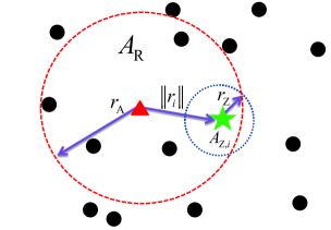
Figure 1: Local neighborhood of the probe transmitting node: each dot represents a node in the network. The triangle is the probe transmitting node and the star is the tested relay (node $i$ in this example). The dashed circle represents the routing zone, $A_{\mathrm{R}}$, with radius $r_{\mathrm{A}}$ centered at the probe transmitting node. The distance between the probe transmitting node and the tested relay is $\|\mathbf{r}_{i}\|$. The threshold zone of node $i$, $A_{\mathrm{Z},i}$, is marked by the small dotted circle with radius $r_{\mathrm{Z}}$ around the tested relay. These circles are used in the proof of Lemma 1 as the maximal distance, which requires special attention. The routing chooses the next-hop that has the maximal routing metric, based on the routing scheme. The difference between schemes is the complexity of the evaluation of the routing metric and its quality (see also Table I).

To derive this low complexity routing scheme, we replace the optimization of (III-A) by an optimization of the following lower bound on (III-A). This lower bound is a slightly modified version of the lower bound proposed by George et al. [11, 32].

Lemma 1.

For each node within the routing zone ($i\in\mathcal{N}_{0}$), denote the disk centered around the node with a radius of $r_{\rm{Z}}=\left(\tfrac{\alpha-2}{\alpha\pi\lambda p_{\mathrm{tx}}}\right)^{1/2}$ as its threshold zone, $A_{\rm{Z},i}$ (see Fig. 1), and denote by $N_{{\rm{Z}},i}$ the number of nodes in the intersection between the threshold zone, $A_{\rm{Z},i}$, and the routing zone (with radius $r_{\rm{A}})$. The function $G(i,M)$ in (12) can be lower bounded using only the known local knowledge, $\mathcal{M}_{0}$, and the system parameters by:

$$G(i,\mathcal{M}_{0})\geq p_{\rm{Z}}(i,\mathcal{M}_{0})\cdot r_{i,0}\log_{2}\left(1+\frac{S_{i,0}}{\bar{J}_{1}^{i}+\bar{J}_{2}^{i}+\sigma_{v}^{2}}\right)$$ (15)

where

$$p_{\rm{Z}}(i,\mathcal{M}_{0})$$ (16)

$$=\begin{cases}(1-p_{\mathrm{tx}})^{N_{{\rm{Z}},i}},&{\rm{if}}\,\ \|\mathbf{r}_{i}\|+r_{\rm{Z}}<r_{\rm{A}}\\ e^{-\lambda p_{\mathrm{tx}}B_{{\rm{T}},i}}(1-p_{\mathrm{tx}})^{N_{{\rm{Z}},i}},&\rm{otherwise}\\ \end{cases}$$

is the probability that there is no interfering transmitting node within the threshold zone,

$$B_{{\rm{T}},i} = r_{\rm{Z}}^{2}\tan^{-1}\Big{(}\tfrac{x_{0}-\|\mathbf{r}_{i}\|}{\sqrt{r_{\rm{Z}}^{2}-(\|\mathbf{r}_{i}\|-x_{0})^{2}}}\Big{)}$$ (17)

$$+(x_{0}-\|\mathbf{r}_{i}\|)\sqrt{-\|\mathbf{r}_{i}\|^{2}+2\|\mathbf{r}_{i}\|x_{0}-x_{0}^{2}+r_{\rm{Z}}^{2}}$$

$$-r_{\rm{A}}^{2}\tan^{-1}\Big{(}\tfrac{x_{0}}{\sqrt{r_{\rm{A}}^{2}-x_{0}^{2}}}\Big{)}-x\sqrt{r_{\rm{A}}^{2}-x_{0}^{2}}$$

and $x_{0}=\frac{r_{\rm{A}}^{2}+\|\mathbf{r}_{i}\|^{2}-r_{\rm{Z}}^{2}}{2\|\mathbf{r}_{i}\|}$. The terms in the denominator are given by

$$\bar{J}_{1}^{i} = \sum\limits_{\begin{subarray}{c}\ell\in\mathcal{N}_{0}\\ \ell:\|\mathbf{r}_{i}-\mathbf{r}_{\ell}\|>\sqrt{\tfrac{\alpha-2}{\alpha\pi\lambda p_{\mathop{\mathrm{tx}}}}}\end{subarray}}p_{\mathrm{tx}}\rho\cdot\|\mathbf{r}_{i}-\mathbf{r}_{\ell}\|^{-\alpha},\vspace{0.5cm}$$ (18)

$$\bar{J}_{2}^{i} = \frac{2(\pi-\theta_{s})\rho\lambda p_{\mathrm{tx}}r_{\rm{Z}}^{2-\alpha}}{\alpha-2}$$

$$+\frac{\rho\lambda p_{\mathrm{tx}}}{\alpha-2}\Big{[}\int_{\theta_{s}}^{2\pi-\theta_{s}}\Big{(}-\|\mathbf{r}_{i}\|\cos(\theta)$$

$$+\sqrt{r_{\rm{A}}^{2}-\|\mathbf{r}_{i}\|^{2}\sin^{2}(\theta)}\Big{)}^{2-\alpha}d\theta\Big{]},$$

where

$$\theta_{s} = \begin{cases}0,&r_{\rm{Z}}+\|\mathbf{r}_{i}\|\leq r_{\rm{A}}\\ \cos^{-1}\big{(}\frac{r_{\rm{A}}^{2}-r_{\rm{Z}}^{2}-\|\mathbf{r}_{i}\|^{2}}{2r_{\rm{Z}}\|\mathbf{r}_{i}\|}\big{)},&r_{\rm{Z}}+\|\mathbf{r}_{i}\|>r_{\rm{A}}\\ \end{cases}.$$ (20)

It may be noted that (1) has closed form expressions for any integer values of $\alpha$ larger than $2$ (detailed expressions for $\alpha=3$ and $\alpha=4$ are given in (C) and (C) in Appendix C).

Proof.

See Appendix A. ∎

The routing function that optimizes (15) is termed Bound Optimal routing (BO) here. This function is given by

$$f_{\rm{BO}}(\mathcal{M}_{0} )=\mathop{\mathrm{argmax}}_{\begin{subarray}{c}i\in\mathcal{N}_{0}\end{subarray}}m_{{}_{\rm{BO}}}(i,\mathcal{M}_{0})$$ (21)

where the routing metric of the BO is

$$m_{{}_{\rm{BO}}}(i,\mathcal{M}_{0})\triangleq p_{\rm{Z}}(i,\mathcal{M}_{0})r_{i,0}\log_{2}\left(1+\frac{S_{i,0}}{\bar{J}_{1}^{i}+\bar{J}_{2}^{i}+\sigma_{v}^{2}}\right).$$ (22)

This metric can be written in a closed form for $\alpha=3,4,5,...$ (when (22) has a closed form expression). However, this can hardly be called a ‘low-complexity’ algorithm (recall that (22) requires the substitution of (16)-(1)).

III-C Narrow Knowledge Statistically-Optimal (NSO) Routing

In the following, we derive a sub-optimal method which is much simpler to evaluate. This method produces nearly the same performance as the SO method, but can be evaluated using a simple, $1$-dimensional lookup table.

As each node has only partial knowledge of the network state, it needs to perform the best routing decision given that knowledge. For this purpose, we use the statistical model of the unknown nodes. The statistical modeling cannot compensate for the unknown data. Nevertheless, it can give us the optimal balancing of the known data.

To reduce the computational complexity, in the following we suggest using only part of the available knowledge (which will be termed narrow knowledge here) when evaluating the routing metric for a specific node. The narrow knowledge of node $j$ on node $i$ is $\mathcal{M}_{j}^{i}=\{r_{i,j},h_{i,j}\}$; i.e., taking only into account the distance to node $i$ and its channel gain (and ignoring the known data on all other neighbors). As we will see, the loss of performance due to the use of narrow knowledge is negligible, whereas the complexity is reduced significantly.

This proposed low-complexity scheme will be denoted as Narrow knowledge Statistically Optimal (NSO). The NSO routing function evaluates $G(i,\mathcal{M}_{0})$ by solely using the available knowledge of the tested relay node, $i$. In mathematical terms, we substitute $G(i,\mathcal{M}_{0})$ by: :

$$G(i,\mathcal{M}_{0}) \approx G_{\mathrm{N}}(i,\mathcal{M}_{0})$$ (23)

$$\triangleq \mathbb{E}_{J|\mathcal{M}_{0}^{i}}\left\{r_{i,0}\log_{2}\left(1+\frac{S_{i,0}}{J_{i,0}+\sigma_{v}^{2}}\right)\Big{|}\mathcal{M}_{0}^{i}\right\}.$$

As $r_{i,0}$ is known given $\mathcal{M}_{0}^{i}$, the optimization of this approximation results in the NSO routing function:

$$f_{\rm{NSO}}(\mathcal{M}_{0})=\mathop{\mathrm{argmax}}_{\begin{subarray}{c}i\in\mathcal{N}_{0}\end{subarray}}m_{{}_{\rm{NSO}}}(i,\mathcal{M}_{0}^{i})$$ (24)

where the routing metric of the NSO is

$$m_{{}_{\rm{NSO}}}(i,\mathcal{M}_{0}^{i})\triangleq r_{i,0}\cdot\mathbb{E}\left\{\log_{2}\left(1+\frac{S_{i,0}}{J_{i,0}+\sigma_{v}^{2}}\right)\Big{|}\mathcal{M}_{0}^{i}\right\}.$$ (25)

Thus, the evaluation of (25) is much simpler than the evaluation of (14), due to the difference in the conditional distribution of the interference, $J_{i,0}$. In the expectation in (25), $J_{i,0}$ is independent of narrow knowledge, and hence, its distribution is identical for all nodes. The complexity of the optimization problem is not large, since the number of points for which the routing needs to calculate their metrics is typically not large. To further simplify the evaluation of the metric in (25), we suggest using the function $q(x_{i})\triangleq\mathbb{E}\Big{\{}\log_{2}(1+\frac{x_{i}}{J_{i,0}+\sigma_{v}^{2}})\Big{|}\mathcal{M}^{i}_{0}\Big{\}}$. Thus, this expectation is only a function of $S_{i,0}$ which can be written as

$$m_{{}_{\rm{NSO}}}(i,\mathcal{M}_{0}^{i})=r_{i,0}\cdot q(S_{i,0})$$ (26)

and the function $q(\cdot)$ can be evaluated as follows.

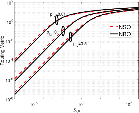
Figure 2: NBO routing metric and NSO routing metric vs. $S_{i,0}$, for various $p_{\mathrm{tx}}\in\{0.01,0.1,0.5\}$ where $r_{i,0}=1$ and $\alpha=4$.

For simple evaluation, the function $q(\cdot)$, which is the only complicated part in the evaluation of the routing metric, can be evaluated once and stored in a lookup table. Thus, the complicated expectation can be evaluated only once, during the network design stage, and the routing metric can be calculated easily in real time using the lookup table. Another alternative would be to evaluate the lookup table on the fly using the interference measurements at the transmitting node (again using the narrow knowledge assumption such that the interference statistics is identical for all nodes).

In the next subsection we present an even simpler routing function for which we can give a simple, closed-form expression of the routing function that does not even require a lookup table.

III-D Narrow Knowledge Bound-Optimal (NBO) Routing

The equivalent of Lemma 1, in (23), becomes:

$$G_{\mathrm{N}}(i,\mathcal{M}_{0})\geq p_{\rm{Z}}(i,\mathcal{M}_{0}^{i})r_{i,0}\log_{2}\left(1+\frac{S_{i,0}}{\gamma+\sigma_{v}^{2}}\right)$$ (27)

with

$$\gamma=\rho\cdot\frac{2}{\alpha}\left(\frac{\alpha\pi\lambda p_{\mathrm{tx}}\Gamma(1+{\frac{2}{\alpha}})}{\alpha-2}\right)^{\frac{\alpha}{2}}$$ (28)

which is a constant that depends on the network parameters. Noting that $p_{\rm{Z}}(i,\mathcal{M}_{0}^{i})$ is identical for all nodes, the NBO routing function that optimizes (27) is given by

$$f_{\rm{NBO}}(\mathcal{M}_{0}) =\mathop{\mathrm{argmax}}_{\begin{subarray}{c}i\in\mathcal{N}_{0}\end{subarray}}m_{{}_{\rm{NBO}}}(i,\mathcal{M}_{0}^{i})$$ (29)

where the routing metric of the NBO is

$$m_{{}_{\rm{NBO}}}(i,\mathcal{M}_{0}^{i})\triangleq r_{i,0}\log_{2}\left(1+\gamma_{b}\cdot S_{i,0}\right)$$ (30)

and $\gamma_{b}=1/(\sigma_{v}^{2}+\gamma)$. In addition, this scheme coincides with the scheme proposed in [16]. While this scheme is not optimal as suggested in [16], we will show in the following section that its performance is quite close to that of the optimal scheme. Since the evaluation of the NBO routing metric is straightforward, we believe that this is indeed a good routing approach for practical networks.

IV Numerical Results

In this section, we present simulation results that demonstrate the efficiency of the proposed routing schemes, where the next hop is selected according to the SO, the BO, the NSO or the NBO routing functions in (III-A), (21), (24) and (29), respectively. In all the simulations we take the number of nodes to have a Poisson distribution with an average of $N_{\rm{nodes}}=300$. The nodes are uniformly distributed in a disk with an area of size $\lambda/N_{\rm{nodes}}$, centered at the probe transmitting node. We also use the bias correction in [33]. To simulate the common interference limited regime, we set $\sigma_{v}^{2}=0$. In this case, the transmitted power, $\rho$, and the node density, $\lambda$, have no effect on performance, and we set $\rho=1$ and $\lambda=1$.

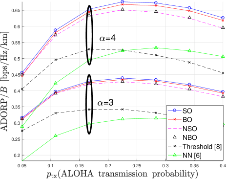
Figure 3: Normalized ADORP as a function of the ALOHA transmission probability for various routing schemes, $\bar{N}_{A}=30$ and $\alpha=3,4$.

To gain some insights into the characteristics of these routing schemes, we start by plotting the routing metrics for the two simpler schemes. Fig. 2 illustrates the NSO and the NBO routing metrics for $\alpha=4$. These schemes are based on narrow knowledge; hence, their routing metric for each node is solely a function of the distance and channel gain to this node. To further simplify the scenario, we consider a tested relay at a distance of $r_{i,0}=1$, such that the metrics are only a function of the channel gain. In the NSO scheme, (26), the resulting metric is the rate: $q(S_{i,0})=\mathbb{E}\left\{\log_{2}\left(1+\frac{S_{i,0}}{J_{i,0}+\sigma_{v}^{2}}\right)\Big{|}\mathcal{M}_{0}^{i}\right\}$, and the aggregate interference can be evaluated by a Monte-Carlo simulation. In the NBO scheme, (30), the resulting metric is the rate: $\log_{2}\left(1+\gamma_{b}\cdot S_{i,0}\right)$ (which is obviously much easier to evaluate than the NSO metric).

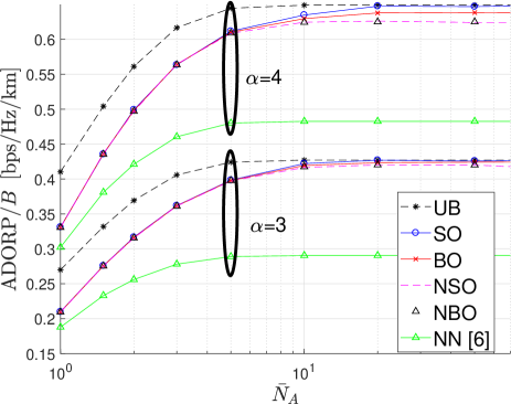
Figure 4: Normalized ADORP as a function of the average number of nodes within the routing zone, $\bar{N}_{A}$, for various routing schemes, $p_{\mathop{\mathrm{tx}}}=0.15$ and $\alpha=3,4$.

The difference between these two metrics is minimal; thus we expect their performance to be quite similar. As expected, both metrics are very sensitive to changes in the channel gain when the channel gain is low. On the other hand, at very high channel gains the achievable rate increases very slowly, and hence the routing metrics are much less sensitive.

The simpler NBO metric considers the interference as a constant, and is less efficient than the NSO. Compared to the NSO metric, the NBO metric gives higher weights to nodes with higher channel gains, $S_{i,0}$, and gives lower weights to nodes with lower channel gains. This difference leads to the small performance gap between NBO and NSO routing, as can be seen in Fig. 3.

Fig. 3 depicts the normalized ADORP (ADORP/$B$) as a function of the ALOHA transmission probability, $p_{\mathrm{tx}}$, for a system with a path loss exponent of $3$ and $4$. All of the proposed schemes perform quite similarly, and achieve the maximum throughput near $p_{\mathop{\mathrm{tx}}}=0.2$. The SO curve serves as an upper bound on the achievable performance, based only on local knowledge. The SO routing function is given in (III-A) and the aggregate interference is evaluated by Monte-Carlo simulations.

The BO scheme, (16)-(21), enables a closed form evaluation of the routing metric, at only negligible loss of performance. ($1.2$% at $\alpha=4$ and $1$% at $\alpha=3$). However, its evaluation still requires high computational complexity. On the other hand, the narrow knowledge schemes (NBO and NSO) are much simpler to evaluate although they incur a slightly larger performance gap ($3.8$% at $\alpha=4$ and $2.6$% at $\alpha=3$). The NBO is even simpler to evaluate and its performance loss compared to the NSO curve is negligible.

For comparison, Fig. 3 also depicts the performance of two geographic routing schemes from the literature: Nearest-Neighbor (NN) routing (e.g., [19, 6]), and Threshold routing [8]. The NN scheme is ranked high among geographic routing schemes. Nevertheless it is inferior to all of our novel schemes. It may be noted that most of the performance gain in our schemes comes from the optimal combination of geographic and channel state knowledge.

The Threshold routing scheme (which was the first published opportunistic relaying scheme) also takes advantage of the CSI to outperform the most-progress-in-radius routing scheme (e.g., [6]). This scheme is an adaptation of Weber et al. [8] to the present setup. In this scheme, the transmitting node first identifies the set of relays for which the power of the desired signal is above a certain threshold. TABLE I summarises the presented routing schemes and the differences among them.

Routing Scheme	Computational Complexity	Use CSI	Performance
Statistically-Optimal (SO)	High	Partial	Optimal
Bound-Optimal (BO)	Medium	Partial	Near optimal
Narrow Knowledge Statistically-Optimal (NSO)	Medium	Narrow	Near optimal
Narrow Knowledge Bound-Optimal (NBO)	Low	Narrow	Near optimal
Threshold [8]	Low	Narrow	Medium
Nearest-Neighbor (NN) [6]	Low	Locations	Low

TABLE I: Major characteristics of the compared routing schemes.

The gain from the use of local knowledge obviously depends on the radius of the routing zone, $r_{A}$. In order to use a scale-free variable, it is convenient to characterize the routing zone area in terms of the average number of nodes within the routing zone, $\bar{N}_{A}\triangleq\lambda\pi r_{A}^{2}$. Fig. 3 presents the case of $\bar{N}_{A}=30$. Fig. 4 presents the normalized ADORP as a function of the average number of nodes within the routing zone for $p_{\mathop{\mathrm{tx}}}=0.15$ and $\alpha=3,4$.

Fig. 4 shows that the performance of all the proposed routing schemes exhibits no significant loss if $\bar{N}_{A}$ is greater than $10$. For smaller routing zones, the gain decreases significantly. However, our schemes outperform the NN for any radius of the routing zone.

It is also crucial to consider the probability that the routing zone is empty. In this case, none of the routing schemes will be able to transfer data, which will inevitably lead to a decrease in performance. To demonstrate this effect, Fig. 4 also depicts an upper bound (UB) on the achievable performance. The UB curve is calculated as the maximum normalized ADORP of the SO curve multiplied by the probability to have a non-empty routing zone, $\mathbb{P}(A_{R}\text{ has at least single node})=1-\exp(-\bar{N}_{A})$.

The upper bound helps us to differentiate between the two effects of increasing the size of the routing zone: better selection and better processing. For small routing zone sizes, each transmitting node has only a few nodes to select from. Hence, any increase in the size of this area can add a better relay and hence improve performance. This effect is saturated around $\bar{N}_{A}=5$, and above that, the only gain is from the better prediction of the interference power. Furthermore, this prediction is generated solely by the SO and BO schemes, so they are the only ones to gain at high $\bar{N}_{A}$.

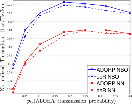
Figure 5: The density of the normalized end-to-end rate distance metric (eeR) as a function of the ALOHA transmission probability in a full network simulation. The figure depicts the performance of the NBO and the NN routing schemes, for a path-loss exponent of $\alpha=3$.

To further demonstrate the advantage of the novel routing schemes, we also performed a complete network simulation, in which messages are routed from sources to destinations according to the mechanism described in Subsection II-C. The simulation was implemented in Matlab, and the results are based on 1000 network realizations. The simulation includes an average of $100$ nodes uniformly distributed over a simulation area of $1000$m². We assume that each node has a home location and an i.i.d. mobility model (e.g., [27]). The mobility follows a symmetric normal distribution with a variance of $2.84$m. This mobility rate represents a low mobility that is only sufficient to unravel the network bottlenecks when choosing a simulation length that depends on $p_{\mathop{\mathrm{tx}}}$ according to $t_{s}=10^{5}/p_{\mathop{\mathrm{tx}}}+8\cdot 10^{5}$ slots. Thus, each simulation was run for a duration of $t_{s}\cdot T$ seconds, where $T$ was the duration of a time slot. Each message contained $20BT$ bits where $B$ was the bandwidth. The messages were not subjected to any delay constraint. The performance was measured by the normalized density of end-to-end rate distance metric (eeR) [16], where we summed the distance-bits product for all successful messages, and divided by the size of the area-time and by the bandwidth. The normalized eeR metric is given by [16, Eq. (9)]:

$$\mathrm{eeR}\triangleq\frac{1}{T_{\mathrm{T}}AB}\sum_{\ell}L_{\ell}K\cdot i_{\ell}$$ (31)

where $A$ is the simulation area, $T_{\mathrm{T}}=t_{s}\cdot T$ is the simulation time, $K=20BT$ is the number of bits per message, $i_{\ell}$ is the successful delivery indicator and $L_{\ell}$ is the distance between source and destination at the time of message generation. Using the ergodic rate approach, a message is assumed to be successfully decoded if it accumulates a mutual information that is equal or larger than $K$ in each of its hops.

Fig. 5 depicts the normalized eeR as a function of the ALOHA transmission probability, $p_{\mathrm{tx}}$, for a system with a path loss exponent of $3$. The figure shows the eeR performance of the NN scheme and the NBO scheme. The figure also shows the relevant normalized ADORP for each scheme. As can be seen, the end-to-end performance indeed converges to the normalized ADORP. Also, as expected from the previous results, the NBO scheme significantly outperforms the NN scheme. The gains vary between $30\%$ to $180\%$.

Fig. 6 depicts the normalized ADORP as a function of the transmission power for various routing schemes, $p_{\mathop{\mathrm{tx}}}=0.15$ and $\alpha=3$. The transmission power is depicted through $\overline{\mathrm{SNR}}_{1}=\rho/\sigma_{v}^{2}$, the averaged SNR for a receiver at $1$ unit distance. As expected, for small SNRs, the normalized ADORP increases linearly with $\overline{\mathrm{SNR}}_{1}$. For $\overline{\mathrm{SNR}}_{1}$ above $-20$dB, the noise becomes negligible, and the networks operate at the interference limited regime. For all SNR values, the proposed schemes outperforms the NN scheme. For very small SNR, the NN becomes close to optimal.

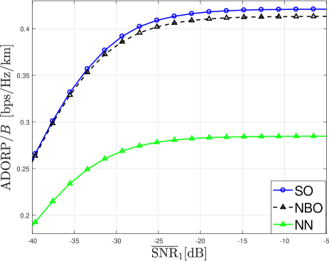
Figure 6: Normalized ADORP as a function of the transmission power, for various routing schemes, $p_{\mathop{\mathrm{tx}}}=0.15$ and $\alpha=3$. The transmission power is depicted through $\overline{\mathrm{SNR}}_{1}=\rho/\sigma_{v}^{2}$, the averaged SNR for a receiver at $1$ unit distance.

V Conclusions

In this paper, we proposed novel routing schemes for WANETs, where the node locations are represented by a PPP. We focus on geographic routing schemes, where the routing decision at each node is based solely on local knowledge on the nodes within its routing zone (geographical locations and channel gains).

In this setup, we were able to formulate the routing objectives as an optimization problem, and to present the routing scheme that solves this optimization problem. The resulting routing scheme requires high computational complexity. Nevertheless, the presentation of the optimal routing scheme is important as it gives an upper bound on the performance of any other routing scheme.

The knowledge of the maximal routing performance also allowed us to present and evaluate three suboptimal low-complexity routing schemes. These schemes were derived by using only part of the available knowledge, by taking a simple lower bound or by combining these two methods. The performance of all three schemes is very close to the performance of the optimal scheme (and in particular at low transmission probability, where the performance gap tends toward zero). Furthermore, the performance of all the proposed routing schemes outperforms the performance of previously published routing schemes.

This paper considers the fast mobility model. While this model is frequently used in stochastic geometry analysis, most practical networks have much tighter delay constraints. Future work should consider a more realistic scenario where messages must be transferred before the network topology changes. In this case, some message buffers in the network may be empty, and the network performance is dominated by its bottlenecks. Hence, the choice of relay must take the state of the buffer, the desired directions of messages in the buffer and the load in each of the potential relays into account. In particular, one can consider an improved routing scheme in which the routing metric suggested above is modified to give proper weights to all of these factors. Such a metric might be able to trade off between the optimization of network throughput and the minimization of the message delay. Future work could also consider the use of multiple antennas at each node.

Appendix A Proof of Lemma 1

The lower bound is based on the use of the law of total expectation, while conditioning on the event that the threshold zone (with radius of $r_{\rm{Z}}$) is free of interferers. Denote by $d_{i}$ the distance between the tested relay (node $i$) and its nearest interfering node. Equation (12) can be written as:

$$G( i,\mathcal{M}_{0})$$

$$= (1-p_{\rm{Z}}(i,\mathcal{M}_{0}))\mathbb{E}\Big{\{}r_{i,0}\log_{2}(1+\tfrac{S_{i,0}}{J_{i,0}+\sigma_{v}^{2}})\Big{|}d_{i}\leq r_{\rm{Z}},\mathcal{M}_{0}\Big{\}}$$

$$+p_{\rm{Z}}(i,\mathcal{M}_{0})\mathbb{E}\Big{\{}r_{i,0}\log_{2}\Big{(}1+\tfrac{S_{i,0}}{J_{i,0}+\sigma_{v}^{2}}\Big{)}\Big{|}d_{i}>r_{\rm{Z}},\mathcal{M}_{0}\Big{\}}$$

$$\geq p_{\rm{Z}}(i,\mathcal{M}_{0})\mathbb{E}\Big{\{}r_{i,0}\log_{2}\Big{(}1+\tfrac{S_{i,0}}{J_{i,0}+\sigma_{v}^{2}}\Big{)}\Big{|}d_{i}>r_{\rm{Z}},\mathcal{M}_{0}\Big{\}}$$

$$\geq p_{\rm{Z}}(i,\mathcal{M}_{0})\cdot r_{i,0}\log_{2}\left(1+\frac{S_{i,0}}{\mathbb{E}\{J_{i,0}|d_{i}>r_{\rm{Z}},\mathcal{M}_{0}\}+\sigma_{v}^{2}}\right)$$

where $p_{\rm{Z}}(i,\mathcal{M}_{0})\triangleq\mathbb{P}(d_{i}>r_{\rm{Z}}\big{|}\mathcal{M}_{0})$ is evaluated in Appendix B, and the last line uses the Jensen inequality. This bound holds for any choice of the threshold radius, $r_{\rm{Z}}$. A useful value for this radius was shown to be [33]: $r_{\rm{Z}}=\sqrt{\tfrac{\alpha-2}{\alpha\pi p_{\mathrm{tx}}\lambda}}$. The rest of the proof focuses on the evaluation of the conditional expectation of the aggregate interference.

We denote by $J_{i,0}(A)$ the aggregate interference at the $i$-th node which is induced only from the transmitting nodes within area $A$. We consider the division of the plane into the non-overlapping areas $A_{\mathrm{Z},i}$, $(\overline{A_{\mathrm{Z},i}}\cap A_{\mathrm{R}})$ and $(\overline{A_{\mathrm{Z},i}}\cap\overline{A_{\mathrm{R}}})$, where $\overline{A}$ denotes the area outside $A$ (see Fig. 1 for an illustration). As we condition on $d_{i}>r_{\rm{Z}}$, we have:

$$\mathbb{E}\{J_{i,0}|d_{i}>r_{\rm{Z}},\mathcal{M}_{0}\} = \mathbb{E}\{J_{i,0}(\overline{A_{\mathrm{Z},i}}\cap A_{\mathrm{R}})|\mathcal{M}_{0}\}$$

$$+\mathbb{E}\{J_{i,0}(\overline{A_{\mathrm{Z},i}}\cap\overline{A_{\mathrm{R}}})|\mathcal{M}_{0}\}.$$

Thus, we define

$$\bar{J}_{1}^{i} \triangleq \mathbb{E}\left\{J_{i,0}(\overline{A_{\rm{Z},i}}\cap A_{\mathrm{R}})|\mathcal{M}_{0}\right\}$$ (34)

$$\bar{J}_{2}^{i} \triangleq \mathbb{E}\left\{J_{i,0}(\overline{A_{\rm{Z},i}}\cap\overline{A_{\mathrm{R}}})|\mathcal{M}_{0}\right\}$$ (35)

and evaluate each expectation separately.

Writing the expectation in (34) more explicitly, we consider $J_{1}^{i}$ to be the aggregate interference at the next relay, which is induced by the transmitting nodes within $(\overline{A_{\rm{Z},i}}\cap A_{\mathrm{R}})$:

$$J_{1}^{i}=\sum\limits_{\begin{subarray}{c}\ell\in\mathcal{N}_{0}\\ \ell:\|\mathbf{r}_{i}-\mathbf{r}_{\ell}\|>\sqrt{\tfrac{\alpha-2}{\alpha\pi\lambda p_{\mathrm{tx}}}}\end{subarray}}g_{\ell}\rho\cdot r_{i,\ell}^{-\alpha}W_{i,\ell},$$ (36)

where $g_{\ell}$ is an indicator function which equals $1$ if the $\ell$-th node is scheduled to serve as a transmitting node, and $\mathbb{E}\{g_{\ell}\}=p_{\mathop{\mathrm{tx}}}$. The expectation of (36), $\bar{J}_{1}^{i}$, can be evaluated by using the statistical independence of transmission decisions:

$$\bar{J}_{1}^{i} = \sum\limits_{\begin{subarray}{c}\ell\in\mathcal{N}_{0}\\ \ell:\|\mathbf{r}_{i}-\mathbf{r}_{\ell}\|>\sqrt{\tfrac{\alpha-2}{\alpha\pi\lambda p_{\mathrm{tx}}}}\end{subarray}}p_{\mathrm{tx}}\rho\cdot\|\mathbf{r}_{i}-\mathbf{r}_{\ell}\|^{-\alpha}.$$ (37)

The evaluation of $\bar{J}_{2}^{i}$ requires a cumbersome analysis of the shape of the area which is seen by the $i$-th node, and its evaluation is given in Appendix C.

Appendix B Evaluation of $p_{\rm{Z}}(i,\mathcal{M}_{0})$

In this appendix we evaluate the probability that there is no interfering transmitting node within the threshold zone, $p_{\rm{Z}}(i,\mathcal{M}_{0})$, which is given in (16). Given $\mathcal{M}_{0}$, the probability $p_{\rm{Z}}(i,\mathcal{M}_{0})$ depends on the number of nodes in the routing zone that lie in the threshold zone of node $i$. Recall that node $j$ lies in the threshold zone of node $i$ if $\|\mathbf{r}_{j}-\mathbf{r}_{i}\|\leq r_{\rm{Z}}$. The evaluation of $p_{\rm{Z}}(i,\mathcal{M}_{0})$ considers two cases:

B-1 $A_{\mathrm{Z},i}$ is located completely within $A_{\mathrm{R}}$

In this case, the probe knows the locations of all nodes within the threshold zone, and can compute the number of nodes within the threshold zone:

$$N_{{\rm{Z}},i}=\sum_{\ell\in\mathcal{N}_{0}}\mathbf{1}_{\{\|\mathbf{r}_{i}-\mathbf{r}_{\ell}\|\leq r_{\rm{Z}}\}}.$$ (38)

The probability that all nodes are receiving nodes is given by $(1-p_{\mathrm{tx}})^{N_{{\rm{Z}},i}}$, which is the first case in (16).

B-2 Part of $A_{\mathrm{Z},i}$ is not located within $A_{\mathrm{R}}$

In this case $A_{\mathrm{Z},i}\cap A_{\mathrm{R}}$ is not necessarily empty, and we need to calculate the probability that a transmitting node is located within $A_{\mathrm{Z},i}$ but outside the routing zone, $A_{\mathrm{R}}$. The area of the threshold zone outside the routing zone is $B_{{\rm{T}},i}\triangleq|\overline{A_{\mathrm{R}}}\cap A_{\mathrm{Z},i}|$. The local knowledge of the probe transmitting node contains no knowledge of the nodes in the area $B_{{\rm{T}},i}$, and we only know that they are characterized by a PPP with density $p_{\mathrm{tx}}\lambda$. The size of $B_{{\rm{T}},i}$ is given in (17). Thus, the probability that this area has no transmitting nodes is given by $e^{-\lambda p_{\mathrm{tx}}B_{{\rm T},i}}$. Multiplying also by the probability that there are no transmitting nodes in $A_{\mathrm{R}}\cap A_{\mathrm{Z},i}$, results in the second case in (16).

Appendix C Evaluation of $\bar{J}_{2}^{i}$

In this appendix we evaluate $\bar{J}_{2}^{i}$, the average interference power from the area $\overline{A_{\rm{Z},i}}\cap\overline{A_{\mathrm{R}}}$ given $\mathcal{M}_{0}$. The final result of this appendix is given in (1). For this calculation, it is convenient to set the axis system so that the origin is located at the tested next relay and the probe transmitting node is located at $x=-\|\mathbf{r}_{i}\|$, $y=0$. Thus, the circle that contains the routing zone, $A_{\mathrm{R}}$, is given by

$$(x+\|\mathbf{r}_{i}\|)^{2}+y^{2} = r_{\rm{A}}^{2}.$$ (39)

Converting to polar coordinates ($x=r\cos(\theta)$ and $y=r\sin(\theta)$), we get

$$r^{2}+2r\cos(\theta)\cdot\|\mathbf{r}_{i}\|+\|\mathbf{r}_{i}\|^{2} = r_{\rm{A}}^{2}.$$ (40)

Hence, the edge of routing zone can be described by

$$r_{0}(\theta)\triangleq-\|\mathbf{r}_{i}\|\cos(\theta)+\sqrt{r_{\rm{A}}^{2}-\|\mathbf{r}_{i}\|^{2}\sin^{2}(\theta)}$$ (41)

and the area can be evaluated by an integral within this area.

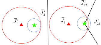
Figure 7: The dashed circle represents the routing zone, $A_{\mathrm{R}}$, centered at the probe transmitting node. The threshold zone of node $i$, $A_{\mathrm{Z},i}$, is marked by the small yellow dotted circle around the tested relay. We evaluate $\bar{J}_{1}^{i}$ and $\bar{J}_{2}^{i}$ which are defined in (34) and (35), respectively. We distinguish between two cases: the left side considers that $A_{\mathrm{Z},i}$ is located completely within $A_{\mathrm{R}}$. The right side considers that part of $A_{\mathrm{Z},i}$ is located outside $A_{\mathrm{R}}$, and thus we use $\bar{J}_{2}^{i}=\bar{J}_{21}^{i}+\bar{J}_{22}^{i}$. The cone width of $\bar{J}_{21}^{i}$ is $2\theta_{s}$. These two cases are used in Appendix C in the evaluation of $\bar{J}_{1}^{i}$ and $\bar{J}_{2}^{i}$.

The characteristic function of $\bar{J}_{2}^{i}$ (the expectation of the aggregate interference at the next relay which is induced by the transmitting nodes within $\overline{A_{\mathrm{Z},i}}\cap\overline{A_{\mathrm{R}}}$) is given by [34]:

$$\Phi_{J_{i,0}}(s)$$ (42)

$$=\exp \Big{(} -2\pi\lambda p_{\mathop{\mathrm{tx}}}\mathbb{E}\Big{\{}\int\int_{\delta(\theta)}^{\infty}(1-e^{-s\rho\lambda p_{\mathop{\mathrm{tx}}}Wr^{-\alpha}}rdrd\theta)\Big{\}}\Big{)}$$

where $\delta(\theta)$ defines the edge of the interference free zone. The expectation over $J_{i,0}$ can be evaluated by substituting $s=0$ into the derivative of $\Phi_{J_{i,0}}(s)$ (see for example [33]). However, we need to distinguish between two cases (See Fig. 7): in the first (left) case, the threshold zone is located completely within the routing zone (i.e., $r_{\rm{Z}}+\|\mathbf{r}_{i}\|\leq r_{\rm{A}}$). In the second (right) case, part of the threshold zone is located outside the routing zone (i.e., $r_{\rm{Z}}+\|\mathbf{r}_{i}\|>r_{\rm{A}}$).

The first case is simpler, and is characterized by $\delta(\theta)=r_{0}(\theta)$, which results in

$$\bar{J}_{2}^{i} = \frac{\partial\Phi_{J_{2}^{i}}(s)}{\partial s}\Big{|}_{s=0}=\rho\lambda p_{\mathop{\mathrm{tx}}}\int_{0}^{2\pi}\int_{r_{0}(\theta)}^{\infty}r^{1-\alpha}drd\theta$$

$$= \frac{\rho\lambda p_{\mathrm{tx}}}{2-\alpha}\Big{[}\int_{0}^{2\pi}\Big{(}-\|\mathbf{r}_{i}\|\cos(\theta)$$

$$+\sqrt{r_{\rm{A}}^{2}-\|\mathbf{r}_{i}\|^{2}\sin^{2}(\theta)}\Big{)}^{2-\alpha}d\theta\Big{]}.$$

In the second case, we start by computing the angle of intersection points between the threshold zone (which is given by $r^{2}=r_{\rm{Z}}^{2}$) and the routing zone. Substituting in (40), we get

$$\cos(\theta) = \frac{r_{\rm{A}}^{2}-r_{\rm{Z}}^{2}-\|\mathbf{r}_{i}\|^{2}}{2r_{\rm{Z}}\|\mathbf{r}_{i}\|}.$$ (44)

Denoting the angle of intersection point by $\theta_{s}\triangleq\cos^{-1}\big{(}\frac{r_{\rm{A}}^{2}-r_{\rm{Z}}^{2}-\|\mathbf{r}_{i}\|^{2}}{2r_{\rm{Z}}\|\mathbf{r}_{i}\|}\big{)}$ we get

$$\delta(\theta)=\begin{cases}R_{Z},&|\theta|<\theta_{s}\\ r_{0}(\theta),&\mathrm{otherwise}\end{cases}.$$ (45)

Thus, we divide the integral into two parts, $\bar{J}_{2}^{i}=\bar{J}_{21}^{i}+\bar{J}_{22}^{i}$, where

$$\bar{J}_{21}^{i} = \rho\lambda p_{\mathop{\mathrm{tx}}}\int_{-\theta_{s}}^{\theta_{s}}\int_{r_{\rm{Z}}}^{\infty}r^{1-\alpha}drd\theta$$

$$= \frac{2\theta_{s}\rho\lambda p_{\mathrm{tx}}r_{\rm{Z}}^{2-\alpha}}{\alpha-2},$$

and

$$\bar{J}_{22}^{i} = \rho\lambda p_{\mathrm{tx}}\int_{\theta_{s}}^{2\pi-\theta_{s}}\int_{r_{0}(\theta)}^{\infty}r^{1-\alpha}drd\theta$$

$$= \frac{\rho\lambda p_{\mathrm{tx}}}{\alpha-2}\Big{[}\int_{\theta_{s}}^{2\pi-\theta_{s}}\Big{(}-\|\mathbf{r}_{i}\|\cos(\theta)$$

$$+\sqrt{r_{\rm{A}}^{2}-\|\mathbf{r}_{i}\|^{2}\sin^{2}(\theta)}\Big{)}^{2-\alpha}d\theta\Big{]}.$$

It may be noted that (C) coincides with (C) if we set $\theta_{s}=0$. Thus, the two different cases can be jointly summarized by Equations (18)-(20).

Unfortunately, the calculations of the integrals in (C) and (C) only have closed form solutions for integer values of $\alpha>2$. However, in the general case, for other non-integer values where $\alpha>2$, these integrals can be evaluated numerically. For example, for $\alpha=3$ we get

$$\bar{J}_{22}^{i} = \rho\lambda p_{\mathop{\mathrm{tx}}}\left[-\frac{2\|\mathbf{r}_{i}\|\sin(\theta_{s})}{r_{\rm{A}}^{2}-\|\mathbf{r}_{i}\|^{2}}\right.$$

$$+\Big{(}E(2\pi-\theta_{s}|\tfrac{\|\mathbf{r}_{i}\|^{2}}{r_{\rm{A}}^{2}})-E(\theta_{s}|\tfrac{\|\mathbf{r}_{i}\|^{2}}{r_{\rm{A}}^{2}})\Big{)}$$

$$\cdot\left.\frac{r_{\rm{A}}^{2}\sqrt{\frac{\|\mathbf{r}_{i}\|^{2}\cos(2\theta_{s})}{r_{\rm{A}}^{2}}-\frac{\|\mathbf{r}_{i}\|^{2}}{r_{\rm{A}}^{2}}+2}}{(r_{\rm{A}}^{2}-\|\mathbf{r}_{i}\|^{2})\sqrt{2r_{\rm{A}}^{2}+\|\mathbf{r}_{i}\|^{2}\cos(2\theta_{s})-\|\mathbf{r}_{i}\|^{2}}}\right]$$

where $E(\phi|k)\triangleq\int_{0}^{\phi}\sqrt{1-k^{2}\sin^{2}(\theta)}d\theta$ is the Elliptic Integral of the second kind. For $\alpha=4$ we get

$$\bar{J}_{22}^{i} = \frac{\rho\lambda p_{\mathrm{tx}}}{4(r_{\rm{A}}^{2}-\|\mathbf{r}_{i}\|^{2})^{2}}\Big{[}-2\|\mathbf{r}_{i}\|\sin(\theta_{s})$$

$$\cdot\sqrt{4r_{\rm{A}}^{2}+2\|\mathbf{r}_{i}\|^{2}\cos(2\theta_{s})-2\|\mathbf{r}_{i}\|^{2}}$$

$$-2r_{\rm{A}}^{2}\tan^{-1}\Big{(}\tfrac{\sqrt{2}\|\mathbf{r}_{i}\|\sin(\theta_{s})}{\sqrt{2r_{\rm{A}}^{2}+\|\mathbf{r}_{i}\|^{2}\cos(2\theta_{s})-\|\mathbf{r}_{i}\|^{2}}}\Big{)}$$

$$+4r_{\rm{A}}^{2}(\pi-\theta_{s})-2\|\mathbf{r}_{i}\|^{2}\sin(2\theta_{s})\Big{]}.$$

References

- [1] E. M. Royer and C.-K. Toh, “A review of current routing protocols for ad hoc mobile wireless networks,” IEEE personal communications, vol. 6, no. 2, pp. 46–55, 1999.
- [2] M. Abolhasan, T. Wysocki, and E. Dutkiewicz, “A review of routing protocols for mobile ad hoc networks,” Elsevier, Ad hoc networks, vol. 2, no. 1, pp. 1–22, 2004.
- [3] F. Baccelli and B. Blaszczyszyn, Stochastic geometry and wireless networks: Volume I theory. Now Publishers Inc, 2010, vol. 1.
- [4] M. Haenggi, J. G. Andrews, F. Baccelli, O. Dousse, and M. Franceschetti, “Stochastic geometry and random graphs for the analysis and design of wireless networks,” IEEE Journal on Selected Areas in Communications, vol. 27, no. 7, pp. 1029–1046, 2009.
- [5] F. Baccelli, B. Blaszczyszyn, and P. Muhlethaler, “On the performance of time-space opportunistic routing in multihop mobile ad hoc networks,” in Proceedings of the 6th IEEE International Symposium on Modeling and Optimization in Mobile, Ad Hoc, and Wireless Networks and Workshops, 2008, pp. 307–316.
- [6] P. H. Nardelli, P. Cardieri, and M. Latva-aho, “Efficiency of wireless networks under different hopping strategies,” IEEE Transactions on Wireless Communications, vol. 11, no. 1, pp. 15–20, 2012.
- [7] D. Torrieri, S. Talarico, and M. C. Valenti, “Multihop routing in ad hoc networks,” in Proceedings of the IEEE Military Communications Conference (MILCOM), 2013, pp. 504–509.
- [8] S. Weber, N. Jindal, R. K. Ganti, and M. Haenggi, “Longest edge routing on the spatial ALOHA graph,” in Proceedings of the IEEE Global Telecommunications Conference (GLOBECOM), 2008, pp. 1–5.
- [9] A. Zanella, A. Bazzi, G. Pasolini, and B. Masini, “On the impact of routing strategies on the interference of ad hoc wireless networks,” IEEE Transactions on Communications, vol. 61, no. 10, pp. 4322–4333, 2013.
- [10] E. Biglieri, J. Proakis, and S. Shamai, “Fading channels: Information-theoretic and communications aspects,” IEEE Transactions on Information Theory, vol. 44, no. 6, pp. 2619–2692, 1998.
- [11] Y. George, I. Bergel, and E. Zehavi, “The ergodic rate density of ALOHA wireless ad-hoc networks,” IEEE Transactions on Wireless Communications, vol. 12, no. 12, pp. 6340–6351, 2013.
- [12] G. George, R. K. Mungara, A. Lozano, and M. Haenggi, “Ergodic spectral efficiency in MIMO cellular networks,” IEEE Transactions on Wireless Communications, vol. 16, no. 5, pp. 2835–2849, 2017.
- [13] A. Rajanna, I. Bergel, and M. Kaveh, “Performance analysis of rateless codes in an ALOHA wireless ad hoc network,” IEEE Transactions on Wireless Communications, vol. 14, no. 11, pp. 6216–6229, 2015.
- [14] A. Larmo, M. Lindström, M. Meyer, G. Pelletier, J. Torsner, and H. Wiemann, “The LTE link-layer design,” IEEE Communications magazine, vol. 47, no. 4, 2009.
- [15] E. Dahlman, S. Parkvall, J. Skold, and P. Beming, 3G evolution: HSPA and LTE for mobile broadband. Academic press, 2010.
- [16] Y. Richter and I. Bergel, “Statistically optimal routing scheme in multihop wireless ad-hoc networks,” in Proceedings of the 28th IEEE Convention of Electrical and Electronics Engineers in Israel (IEEEI), 2014.
- [17] J. G. Andrews, S. Weber, M. Kountouris, and M. Haenggi, “Random access transport capacity,” IEEE Transactions on Wireless Communications, vol. 9, no. 6, pp. 2101–2111, 2010.
- [18] Y. Richter and I. Bergel, “Optimal and suboptimal routing based on partial CSI in wireless ad-hoc networks,” in Proceedings of the 16th IEEE International Workshop on Signal Processing Advances in Wireless Communications (SPAWC), 2015, pp. 191–195.
- [19] M. Haenggi, “On routing in random Rayleigh fading networks,” IEEE Transactions on Wireless Communications, vol. 4, no. 4, pp. 1553–1562, 2005.
- [20] J. Arnbak and W. Van Blitterswijk, “Capacity of slotted ALOHA in Rayleigh-fading channels,” IEEE Journal on Selected Areas in Communications, vol. 5, no. 2, pp. 261–269, 1987.
- [21] F. Baccelli, B. Blaszczyszyn, and P. Muhlethaler, “An ALOHA protocol for multihop mobile wireless networks,” IEEE Transactions on Information Theory, vol. 52, no. 2, pp. 421–436, 2006.
- [22] T. Yoo and A. Goldsmith, “Capacity and power allocation for fading MIMO channels with channel estimation error,” IEEE Transactions on Information Theory, vol. 52, no. 5, pp. 2203–2214, 2006.
- [23] J. Baltersee, G. Fock, and H. Meyr, “An information theoretic foundation of synchronized detection,” IEEE Transactions on Communications, vol. 49, no. 12, pp. 2115–2123, 2001.
- [24] M. Guillaud, D. T. Slock, and R. Knopp, “A practical method for wireless channel reciprocity exploitation through relative calibration,” in ISSPA, 2005, pp. 403–406.
- [25] H.-W. Liang, W.-H. Chung, and S.-Y. Kuo, “FDD-RT: A simple CSI acquisition technique via channel reciprocity for FDD massive MIMO downlink,” IEEE Systems Journal, 2016.
- [26] M. Grossglauser and D. Tse, “Mobility increases the capacity of ad-hoc wireless networks,” in Proceedings of the IEEE Twentieth Annual Joint Conference of the IEEE Computer and Communications Societies INFOCOM, vol. 3, 2001, pp. 1360–1369.
- [27] Z. Gong and M. Haenggi, “The local delay in mobile Poisson networks,” IEEE Transactions on Wireless Communications, vol. 12, no. 9, pp. 4766–4777, 2013.
- [28] B. Błaszczyszyn and P. Mühlethaler, “Random linear multihop relaying in a general field of interferers using spatial ALOHA,” IEEE Transactions on Wireless Communications, vol. 14, no. 7, pp. 3700–3714, 2015.
- [29] N. Ravindran, P. Wu, J. Blomer, and N. Jindal, “Optimized multi-antenna communication in ad-hoc networks with opportunistic routing,” in Proceedings of the 44 IEEE Asilomar Conference on Signals, Systems and Computers), 2010, pp. 1593–1597.
- [30] D. Li, C. Yin, C. Chen, and S. Cui, “A selection region based routing protocol for random mobile ad hoc networks,” in Proceedings of the IEEE GLOBECOM Workshops, 2010, pp. 104–108.
- [31] S. Srinivasa and M. Haenggi, “Path loss exponent estimation in large wireless networks,” in Proceedings of the Information Theory and Applications Workshop. IEEE, 2009, pp. 124–129.
- [32] Y. George, I. Bergel, and E. Zehavi, “Upper bound on the ergodic rate density of ALOHA wireless ad-hoc networks,” IEEE Transactions on Wireless Communications, vol. 14, no. 6, pp. 3004–3014, 2015.
- [33] Y. Richter and I. Bergel, “Analysis of the simulated aggregate interference in random ad-hoc networks,” in Proceedings of the 15th IEEE International Workshop on Signal Processing Advances in Wireless Communication (SPAWC), 2014.
- [34] J. Venkataraman, M. Haenggi, and O. Collins, “Shot noise models for outage and throughput analyses in wireless ad hoc networks,” in Proceedings of the IEEE Military Communications Conference (MILCOM), 2006, pp. 1–7.