Factorization of Linear Quantum Systems
with Delayed Feedback

Abstract.

We consider the transfer functions describing the input-output relation for a class of linear open quantum systems involving feedback with nonzero time delays. We show how such transfer functions can be factorized into a product of terms which are transfer functions of canonical physically realizable components. We prove under certain conditions that this product converges, and can be approximated on compact sets. Thus our factorization can be interpreted as a (possibly infinite) cascade. Our result extends past work where linear open quantum systems with a state-space realization have been shown to have a pure cascade realization [Nurdin, H. I., Grivopoulos, S., & Petersen, I. R. (2016). The transfer function of generic linear quantum stochastic systems has a pure cascade realization. Automatica, 69, 324-333.]. The functions we consider are inherently non-Markovian, which is why in our case the resulting product may have infinitely many terms.

1. Overview

We will be concerned here with a class of non-Markovian linear open quantum systems. Specifically, we will construct this class of systems by adding delayed feedback to a (Markovian) finite-dimensional open quantum system. After this procedure, the transfer function may not correspond to a rational function. We will show that under certain conditions the input-output relationship of such systems can be realized as a (possibly infinite) cascade of canonical components. To do this, we will factorize the transfer function into an infinite product of canonical terms, where each term corresponds to a physically realizable component. Each such term will be identified using a pair of poles and zeros. The delayed-feedback system can then be approximated using a finite truncation of the infinite product. One application of our result is providing experimentalists with a method to generate a cascade network of canonical terms replicating the behavior of a system with delayed feedback.

Our work provides an extension of some prior papers, and is closely related to others. In [8] and [14], the authors obtain a cascade realization from a given linear quantum stochastic system. Our work here can be considered a natural extension in the case of delayed feedback. Isolated loops with time delays are also discussed in the context of linear quantum systems in [4]. In [20], a cascade realization is given for passive linear systems with delayed feedback. In that case, it suffices to consider only the input-output relationship for the annihilation operators. In the current paper we consider more generally quantum linear systems which may not be passive. In order to characterize the transfer function for such a system, we must consider the input-output relationship between both the creation and annihilation operators, since the system may have squeezing effects.

There are also approaches that have been developed for simulating coherent feedback systems with time delays for the case when the system may be in general nonlinear. In [7], a series of cascaded systems is introduced, such that the system is driven by past versions of itself. Later in [21], this work was extended to include the case of multiple delays of different durations. In [15], matrix product states were used study the dynamics of coherent feedback networks with significant delays. These approaches differ from our approach where a cascade of canonical terms is constructed in the frequency domain (which is well-defined for linear systems) by considering the shape of the transfer function near the zeros and poles.

In the case of rational transfer functions, properties of the the state-space representation matrices can be used to determine if a system is physically realizable. It has been shown in  [18] that under some non-degeneracy assumptions these conditions are equivalent to certain properties of the transfer function in the frequency domain. Essentially, as long as the state-space realization matrices are in ‘doubled-up’ form and certain non-degeneracy conditions hold, the physical realizability of the system is equivalent to the transfer function having the $J$-unitary property (and a property preventing static squeezing). Once delayed feedback is incorporated, although the system remains linear, it loses its Markovian property and no longer has a corresponding state-space representation. We introduce an extension of the frequency domain constraints for physical realizability and utilize it to obtain our factorization under certain assumptions, stated in Section 4.1 and in the non-degeneracy conditions in the hypothesis of Theorems 7.1 and 7.2. Some of the assumptions follow from our construction starting with a finite-dimensional physically realizable system (Assumptions 1 and 2), and others are introduced for simplicity (Assumptions 4, 5, and 6). Assumption 3 ensures the network does not have effectively time-delayed feed-forward terms. An analysis similar to the one in [20] can be used to isolate such terms, but this is outside the scope of our paper.

In Section 2, we introduce the various definitions and notation we use throughout. In Section 3 we introduce (finite-dimensional) linear quantum stochastic systems and discuss the physical realizability conditions of transfer functions. In Section 4 we construct a delayed-feedback network and state assumptions we make throughout. In Section 5 we provide some properties of our delayed-feedback network. In Section 6 we provide theorems that relate the transfer function of the delayed-feedback network with a simpler transfer function resulting from replacing the internal components of the network with static components. These theorems will be useful in providing convergence results. In Section 7 we introduce physically realizable canonical transfer functions having only two poles and two zeros. Finally, in Section 8, we provide our factorization result.

2. Definitions

The definitions below are frequently used in the literature (e.g. [5],[6],[18]).

definition 2.1.

The signature matrix $J$ of dimension $2n$ is a diagonal matrix with alternating $(+1,-1)$ on its diagonal.

definition 2.2.

For a matrix $M$ we use the notation $M^{\flat}=JM^{\#}J$.

definition 2.3.

A doubled-up matrix has the form

(1) $$\breve{M}=\Delta(M_{-},M_{+})\equiv\begin{pmatrix}M_{-}&&M_{+}\\ M_{+}^{\#}&&M_{-}^{\#}\end{pmatrix}.$$

A doubled-up column vector has the form

(2) $$\breve{v}=\begin{pmatrix}v\\ v^{\#}\end{pmatrix}.$$

Here $M^{\#},v^{\#}$ denote the elementwise conjugates of $M,v$.

definition 2.4.

A matrix $M$ is $J$-unitary iff

(3) $$MJM^{\dagger}=M^{\dagger}JM=J.$$

definition 2.5.

A matrix-valued function $M(z)$ is $J$-unitary iff

(4) $$M(z)JM(z)^{\dagger}=M(z)^{\dagger}JM(z)=J,$$

for z on the imaginary axis.

It a transfer function is $J$-unitary and meromorphic on the plane, then satisfies $M(z)JM(-\overline{z})^{\dagger}=J$ on its domain.

It will be convenient to permute the annihilation and creation operators using the symmetric permutation matrix $P$, exchanging the indices the first $N$ indices, $1,2,...,N$ with the odd indices up to $2N$, and exchanging the last $N$ indices $N+1,...,2N$ with the even indices up to $2N$. When this is the case (Section 4 and beyond) it will be understood that doubled-up matrices will have the form $\tilde{M}=PMP^{T}$ instead. For example, the matrix

(5) $$M=\Delta(M_{-},M_{+})=\begin{pmatrix}M_{-,11}&M_{-,12}&M_{+,11}&M_{+,12}\\ M_{-,21}&M_{-,22}&M_{+,21}&M_{+,22}\\ M_{+,11}^{\#}&M_{+,12}^{\#}&M_{-,11}^{\#}&M_{-,12}^{\#}\\ M_{+,21}^{\#}&M_{+,22}^{\#}&M_{-,21}^{\#}&M_{-,22}^{\#}\end{pmatrix}$$

would be re-arranged as

(6) $$PMP^{T}=\begin{pmatrix}M_{-,11}&M_{+,11}&M_{-,12}&M_{+,12}\\ M_{+,11}^{\#}&M_{-,11}^{\#}&M_{+,12}^{\#}&M_{-,12}^{\#}\\ M_{-,21}&M_{+,21}&M_{-,22}&M_{+,22}\\ M_{+,21}^{\#}&M_{-,21}^{\#}&M_{+,22}^{\#}&M_{-,22}^{\#}\\ \end{pmatrix}.$$

definition 2.6.

We will say a rational transfer function is in ‘doubled-up’ form when it has a realization given by matrices $A,B,C,D$, (i.e. $T(z)=D+C(zI-A)^{-1}B$), where each is in doubled-up form.

definition 2.7.

Given a dimension $b$, let

(7) $$\Sigma_{b}=\begin{pmatrix}0&&I_{b}\\ I_{b}&&0\end{pmatrix}$$

The subscript $b$ will be dropped when the dimension is clear from context.

It will be understood that when the annihilation and creation ports are permuted as discussed above, we will use $\tilde{\Sigma}=P\Sigma P^{T}$ instead.

remark 2.1.

A matrix $M$ is doubled-up if and only if it satisfies

(8) $$M\Sigma=\Sigma M^{\#},$$

2.1. Zeros and poles

In the literature, there are different definitions for zeros and poles of a matrix-valued function. We will describe two kinds of definitions, which we will denote respectively by (I) and (II):

definition 2.8.

A complex number z is called a pole(I) of $A(z)$ if it is a pole of one of the entries of $A(z)$, and z is called a zero(I) of $A(z)$ if it is a pole(I) of $A(z)^{-1}$. This is the definition used in Ref. [16].

definition 2.9.

A complex number z is called a pole(II) of $A(z)$ if it is a pole of $\det A(z)$, and z is called a zero(II) of $A(z)$ if it is a zero of $\det A(z)$. This is the definition used in Ref. [20]. Note that definition 2.9 implies 2.8, but not the converse.

remark 2.2.

The definitions (I) could have a pole and a zero in the same location. Instead, for definitions (II) this cannot occur. If zeros (I) and poles (I) do not occur in the same location, then the definitions (I) and (II) coincide. For simplicity, we will assume that is the case (Assumption 5).

definition 2.10.

(eigenvectors at zeros and poles, adapted from Ref. [16]) Suppose $z_{0}$ is a zero(I) of matrix valued function $A(z)$. A nonzero column vector $x_{1}$ is called an eigenvector of $A(z)$ at $z_{0}$ if there exist column vectors $(x_{2},x_{3},\ldots)$ such that $f(z)=A(z)\sum_{j=0}^{\infty}x_{j+1}(z-z_{0})^{j}$ is analytic at $z_{0}$ and has a zero at $z_{0}$. We will say the order of the zero of $A(z)$ with eigenvector $x_{1}$ at $z_{0}$ is the order of $f(z)$ at $z_{0}$.

Similarly, if $z_{0}$ is a pole of $A(z)$, then $y_{1}$ is a pole vector of $A(z)$ at $z_{0}$ (we will sometimes say an eigenvector at the pole) if there exist vectors $(y_{2},y_{3},\ldots)$ such that $g(z)=\sum_{j=0}^{\infty}y_{j+1}(z-z_{0})^{j}A(z)^{-1}$ is analytic at $z_{0}$ and has a zero at $z_{0}$. We will say the order of the pole of $A(z)$ with eigenvector $y_{1}$ at $z_{0}$ is the order of $g(z)$ at $z_{0}$.

remark 2.3.

Definition 2.10 is most intuitive in the case where zeros and poles do not overlap and have order and multiplicity one. In this case, the auxiliary vectors $(x_{2},x_{3},\ldots)$ and $(y_{2},y_{3},\ldots)$ are unnecessary, and an eigenvector $x_{1}$ for zero(I) $z_{0}$ occurs when $f(z)=A(z)x_{1}$ is zero-valued at $z_{0}$, and a pole vector $y_{1}$ for pole(I) $z_{0}$ occurs when $g(z)=y_{1}A(z)^{-1}$ is zero-valued at $z_{0}$.

3. Finite-Dimensional Linear Quantum Stochastic Systems (LQSS)

We provide a brief introduction here for (finite-dimensional) LQSS. Consider a system with a finite-dimensional state $x(t)$ driven by a bosonic input field $b_{\text{in}}(t)$ and generating a bosonic output field $b_{\text{out}}(t)$. The most general form of a linear system preserving the commutation relations in the input-output relationship has the form

(9) $$\frac{{\rm d}}{{\rm d}t}x =(A_{-}x+A_{+}x^{\#})+(B_{-}b_{\text{in}}+B_{+}b_{\text{in}}^{\#})$$

(10) $$b_{\text{out}} =(C_{-}x+C_{+}x^{\#})+(D_{-}b_{\text{in}}+D_{+}b_{\text{in}}^{\#}).$$

Using the notation $\breve{M}=\Delta(M_{-},M_{+})$ for matrices and $\breve{v}=(v,v^{\#})^{T}$ for vectors (e.g. as used in [6]), this can be written as

(11) $$\frac{{\rm d}}{{\rm d}t}\breve{x} =\breve{A}\breve{x}+\breve{B}\breve{b}_{\text{in}}$$

(12) $$\breve{b}_{\text{out}} =\breve{C}\breve{x}+\breve{D}\breve{b}_{\text{in}}.$$

The matrices $\breve{A},\breve{B},\breve{C},\breve{D}$ must satisfy special physical realizability constraints (e.g. Ref. [18]).

The input-output relationship may be characterized by the transfer function of the system. This function is obtained by taking the Laplace transform of the equations of motion, defined by $Y(z)=\int_{0}^{\infty}e^{-zt}y(t)dt$. Letting $X(z),B_{\text{in}}(z)$, and $B_{\text{out}}(z)$ be the Laplace transforms of $x(t),b_{\text{in}}(t)$, and $b_{\text{out}}(t)$, respectively, and eliminating $X(z)$ from the resulting equations, one obtains $B_{\text{out}}(z)=T(z)B_{\text{in}}(z)$, where $T(z)=\breve{D}+\breve{C}(zI-\breve{A})^{-1}\breve{B}$. In Section 4 we will build upon finite-dimensional LQSS, introducing time-delayed feedback. We will do so by considering the Laplace transform of the newly constructed network including the time-delayed feedback.

Theorem 4 in Ref. [18] states an equivalent condition for physical realizability in the frequency domain when $\breve{A},\breve{B},\breve{C},\breve{D}$ are doubled up in the sense of Eq. (1) and assuming the state space realization is minimal and the eigenvalues of $\breve{A}$ satisfy $\lambda_{i}(\breve{A})+\lambda_{j}(\breve{A})\neq 0$ (a condition which always holds for stable systems with $A<0$). With these assumptions the system is physically realizable if and only if

1. The transfer function $T(z)$ is $J$-unitary.

2. The matrix $\breve{D}$ has form $\breve{D}=\Delta(S,0)$ for a unitary matrix $S$.

The first condition ensures the commutation relations are preserved, while the second condition ensures there is no static (infinite-bandwidth) squeezing in the system (this would lead to energy divergences and breaks the Hudson-Parthasarathy quantum stochastic calculus). We will show in the following sections that the state space matrices being doubled-up and the first condition above can be generalized for the cases when there is no finite-dimensional state-space. However, the second condition has no clear analogue (see in particular the discussion in Section 8.4).

4. Linear Quantum Stochastic Systems with Delayed Feedback

We begin with an LQSS as described in Section 3 having $2(N+M)$ inputs and $2(N+M)$ outputs. $N+M$ of the input/output ports correspond to the input/output annihilation field, and the other $N+M$ of the input/output ports correspond to the input/output creation field. For convenience, we permute the input and output ports, so that the odd-labeled ports correspond to the creation fields and the even ports to the creation fields.

We assume this transfer function corresponds to a finite-dimensional (i.e. it is a proper rational function) throughout (see Assumption 1). The transfer function of this system has form

(13) $$T(z)=\begin{pmatrix}T_{1}(z)&&T_{2}(z)\\ T_{3}(z)&&T_{4}(z)\end{pmatrix},$$

where the matrix has been partitioned into blocks of size $2N\times 2N$, $2N\times 2M$, $2M\times 2N$, and $2M\times 2M$.

Remark: A complex-valued function on the extended plane is a proper rational function if and only if it is meromorphic on the extended complex plane and analytic at infinity. This applies to the components of $T(z)$, and will be important throughout.

Next, we add delays with feedback to the system. In the case for linear quantum systems, we use

(14) $$E(z) =\text{diag}(e^{-T_{1}z},e^{-T_{1}z},...,e^{-T_{M}z},e^{-T_{M}z}).$$

(15) $$\tilde{T}(z) =T_{1}(z)+T_{2}(z)E(z)(I-T_{4}(z)E(z))^{-1}T_{3}(z)$$

(16) $$=T_{1}(z)+T_{2}(z)(E(-z)-T_{4}(z))^{-1}T_{3}(z).$$

Each time delay occurs in two terms of $E(z)$, once for annihilation and once for the creation field. Notice that $E(-z)=E(z)^{-1}$ because of its special form. This notation will be used throughout. Figure 1 shows conceptually how the blocks $T_{i}(z)$ for $i=1,2,3,4$ are used to construct the new transfer function $\tilde{T}(z)$. It can be shown $E(z)$ is $J$-unitary. This is a similar setup to [5]. This term can be derived from the Fourier transform on an linear quantum system with delayed input ports.

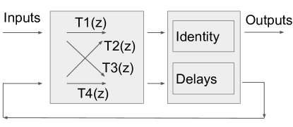
Figure 1. The setup of the network with delayed feedback constructed in Eq. (14). The arrows in the left box indicate how the blocks $T_{i}(z)$ for $i=1,2,3,4$ relate the inputs and outputs of $T(z)$ to the inputs and outputs of $\tilde{T}(z)$ with respect to the time delays.

4.1. Assumptions

These are assumptions we will make throughout.

1. The transfer function $T(z)$ is a proper rational function. This means that each of its components can be expressed as a ratio of polynomials, and that the degree of the numerator is never greater than the denominator. Notice in particular this implies $T(z)$ is analytic at infinity.

2. The transfer function $T(z)$ is doubled-up and $J$-unitary.

3. There is some $C$ so that for $\{z:|z|>C\}$, $T_{2}(z),T_{3}(z),T_{4}(z)$ are invertible, and their singular values are bounded away from zero by some positive constant. This generalizes the condition in section 8.1 of reference [20] where the network components were static and passive. Here, $T_{4}(z)$ replaces the static matrix $M_{1}$. This condition on $T_{4}(z)$ excludes a series product with delay $B\triangleleft A$. For systems that do not satisfy this assumption, an approach similar to that used in [20] may be used in order to separate out terms corresponding to feedforward time delays. The condition on $T_{2}(z)$ and $T_{3}(z)$ allows us to prove Lemma 6.1.

4. periods $T_{1},...,T_{N}$ are commensurate. This suffices for practical purposes, and simplifies some of the proofs.

5. Zeros(I) and poles(I) from Definition 2.8 do not occur in the same location.

6. For simplicity, suppose that whenever we find a zero or pole of a transfer function of interest, there is up to a scalar only one eigenvector at the zero/pole (i.e. the multiplicity of each zero/pole is one). Also, each zero/pole has order one in the sense of Definition 2.10.

There are additional specific non-degeneracy assumptions discussed in Section 7.2.

5. Properties of transfer functions

Claim 5.1.

• If two transfer functions are $J$-unitary, then so is their product.

• If two transfer functions can be written in doubled-up notation, then so can their product.

• The inverse of a $J$-unitary function is $J$-unitary.

proofs: Direct computation.

Claim 5.2.

If a rational transfer function is doubled-up, then so is its inverse.

proof: This follows using a realization of the inverse of a transfer function, which is valid when $D$ is invertible (see e.g. reference [12]):

Denoting a transfer function by $G(z)=D+C(zI-A)^{-1}B$ by $\left(\begin{array}[]{c|c}A&B\\ \hline\cr C&D\\ \end{array}\right)(z)$, its inverse is

(21) $$\left(\begin{array}[]{c|c}A&B\\ \hline\cr C&D\\ \end{array}\right)^{-1}(z)=\left(\begin{array}[]{c|c}A-BD^{-1}C&-BD^{-1}\\ \hline\cr D^{-1}C&D^{-1}\end{array}\right)(z).$$

From this one sees that the matrices for the state space representation of the inverse are also doubled up. $\blacksquare$

Claim 5.3.

$J$-unitarity is preserved under concatenation, series, and feedback products.

proof: The case for the concatenation product is trivial:

(22) $$\begin{bmatrix}T_{1}(z)&0\\ 0&T_{2}(z)\end{bmatrix}J\begin{bmatrix}T_{1}(z)&0\\ 0&T_{2}(z)\end{bmatrix}^{\dagger}=\begin{bmatrix}T_{1}(z)J_{1}T_{1}(z)^{\dagger}&0\\ 0&T_{2}(z)J_{2}T_{2}(z)^{\dagger}\end{bmatrix}=\begin{bmatrix}J_{1}&0\\ 0&J_{2}\end{bmatrix}=J$$

The series product follows from associativity:

(23) $$\bigl{(}T_{1}(z)T_{2}(z)\bigr{)}J\bigl{(}T_{1}(z)T_{2}(z)\bigr{)}^{\dagger}=T_{1}(z)\bigl{(}T_{2}(z)JT_{2}(z)^{\dagger}\bigr{)}T_{1}(z)^{\dagger}=T_{1}(z)JT_{1}(z)^{\dagger}=J$$

The only nontrivial case is the feedback product. Here we start with a transfer function

(24) $$T(z)=\begin{bmatrix}T_{1}(z)&T_{2}(z)\\ T_{3}(z)&T_{4}(z)\end{bmatrix}$$

$J$-unitarity implies:

$$T_{1}JT_{1}^{\dagger}+T_{2}JT_{2}^{\dagger} =J$$

$$T_{1}JT_{3}^{\dagger}+T_{2}JT_{4}^{\dagger} =0$$

$$T_{3}JT_{1}^{\dagger}+T_{4}JT_{2}^{\dagger} =0$$

(25) $$T_{3}JT_{3}^{\dagger}+T_{4}JT_{4}^{\dagger} =J$$

Expanding $TJT^{\dagger}$ using $T=T_{1}+T_{2}(1-T_{4})^{-1}T_{3}$, and using the rules (25) to trade $T_{1},T_{3}$ for $T_{2},T_{4}$, we find:

$$T(z)JT(z)^{\dagger} =J+T_{2}(1-T_{4})^{-1}\Bigl{[}-(1-T_{4})J(1-T_{4}^{\dagger})-T_{4}J(1-T_{4}^{\dagger})$$

(26) $$\qquad\qquad\qquad\qquad\quad-(1-T_{4})JT_{4}^{\dagger}-T_{4}JT_{4}^{\dagger}+J\Bigr{]}(1-T_{4}^{\dagger})^{-1}T_{2}^{\dagger}$$

The terms inside the square brackets vanish, leaving $J$, so $T(z)$ is $J$-unitary. $\blacksquare$

Claim 5.4.

If $T(z)$ is unitary ($J$-unitary), then so is $\tilde{T}(z)$ defined above.

proof: $\tilde{T}(z)$ is be obtained from $T(z)$ and $E(z)$ using concatenation, series and feedback operations. Since these preserve $J$-unitarity, $\tilde{T}(z)$ must be $J$-unitary as well. $\blacksquare$

5.1. Properties of the Roots and Poles of $\tilde{T}(z)$.

Claim 5.5.

If a transfer function $T(z)$ is $J$-unitary, its (complex) poles and zeros come in pairs of the form $z_{0},-\overline{z}_{0}$. Furthermore, suppose $x$ is an eigenvector of the zero $z_{0}$ of $T(z)$ in the sense of [16]. Then $x^{\dagger}J$ is an eigenvector of the pole $-\overline{z}_{0}$ at $T(z)$ in the sense of [16].

proof: This follows from $T(z)JT(-\overline{z})^{\dagger}=J$. In particular, we can re-arrange to get

(27) $$T^{-1}(z)=JT^{\dagger}(-\overline{z})J.$$

Since $z_{0}$ is an eigenvalue of $T(z)$ with eigenvector $x$, there are some vectors $x_{2},x_{3},...$ such that $T(z)[x+x_{2}(z-z_{0})+...]$ is analytic with a zero at $z_{0}$. Multiplying on the left of Eq. (27) by $x^{\dagger}J+x_{2}^{\dagger}J(z+\overline{z_{0}})+...$, we find the expression is analytic with a zero at $-\overline{z}_{0}.$ $\blacksquare$

Claim 5.6.

If a rational transfer function $T(z)$ is doubled-up, then it satisfies

(28) $$T(z)=\Sigma T(\overline{z})^{\#}\Sigma.$$

proof: $T(z)$ is doubled-up if and only if for each matrix $R$ among $A,B,C,D$, $\Sigma R\Sigma=R^{\#}$. The rest is straightforward algebra. $\blacksquare$

The property $T(z)=\Sigma T(\overline{z})^{\#}\Sigma$ generalizes the notion of a doubled-up transfer function for a finite dimensional system to more general functions (i.e. $T(z)$ is no longer required to be rational).

Claim 5.7.

Given a transfer function $T(z)$ satisfying the property $T(z)=\Sigma T(\overline{z})^{\#}\Sigma$, if $z_{0}$ is a zero of $T(z)$, then so is $\overline{z_{0}}$. If $x$ is an eigenvector of $T(z)$ at $z_{0}$, then $\Sigma x^{\#}$ is an eigenvector of $T(z)$ at $\overline{z_{0}}$.

Similarly, if $z_{0}$ is a pole of $T(z)$, then so is $\overline{z_{0}}$. If $x$ is an the eigenvector of $T(z)$ at $z_{0}$, then $\Sigma x^{\#}$ is an eigenvector of $T(z)$ at $\overline{z_{0}}$.

proof: Since $z_{0}$ is a zero of $T(z)$, there are some vectors $x_{2},x_{3},...$ such that $T(z)[x+x_{2}(z-z_{0})+...]$ is analytic with a zero at $z_{0}$. Applying the property $T(z)=\Sigma T(\overline{z})^{\#}\Sigma$, and using the fact that $f(z)$ is analytic if and only if $\overline{f(\overline{z})}$ is analytic, we obtain the desired result.

The proof for the poles follows similarly. $\blacksquare$

Corollary 5.1.

If the zero $z_{0}$ with eigenvector $x$ is real, then $y=\Sigma x^{\#}$ is also an eigenvector at $z_{0}$.

Claim 5.8.

Suppose $T(z)$ is a rational transfer function that can be written in doubled-up form. If $z$ is a pole of $\tilde{T}(z)$, then so is $\overline{z}$.

proof: This follows from the fact that $\Sigma\tilde{T}(\overline{z})^{\#}\Sigma=\tilde{T}(z)$, proved using the identities $\Sigma E(z)\Sigma=E(\overline{z})^{\#}$ and $\Sigma A\Sigma=A^{\#}$, etc., below:

$$\Sigma\tilde{T}(\overline{z})^{\#}\Sigma =\Sigma\left[D^{\#}+C^{\#}(zE(-\overline{z})^{\#}-A^{\#})^{-1}B^{\#}\right]\Sigma$$

(29) $$=D+C(zE(-z)-A)^{-1}B=\tilde{T}(z)$$

From here we use Claim 5.7 to show that $\bar{z}$ is also a pole of $\tilde{T}(z)$. $\blacksquare$

5.2. The poles of $\tilde{T}(z)$ have bounded real part

We begin by showing that if $T_{4}(z)$ has singular values bounded away from zero for all $z\in\{|z|>C\}$ for some $C$ (Assumption 3), then the poles of $\tilde{T}(z)$ have bounded real part. We will also use that $T_{4}(z)$ is a rational function (Assumption 1), and therefore its singular values are also bounded from above.

The original transfer function $T(z)$ is rational, so it has a finite number of poles. Therefore for the purposes of showing a bound for the real part of the poles of $\tilde{T}(z)$, we can ignore the poles of $T(z)$. The remaining poles of $\tilde{T}(z)$ can only occur when $(E(-z)-T_{4}(z))^{-1}$ has a pole. We will obtain our desired bounds using the following lemma:

Lemma 5.1.

Given matrices $A,B$ with singular values satisfying $\sigma_{\min}(A)-\sigma_{\max}(B)>\epsilon$, the matrix $A-B$ is invertible, and $\sigma_{\min}(A-B)>\epsilon$.

proof: The key step employs the triangle inequality:

$$\sigma_{\min}(A-B) =\inf_{\|x\|=1}\|(A-B)x\|\geq\inf_{\|x\|=1}(\|Ax\|-\|Bx\|)$$

(30) $$\geq\inf_{\|x\|=1}\|Ax\|-\sup_{\|x\|=1}\|Bx\|=\sigma_{\min}(A)-\sigma_{\max}(B)>\epsilon.$$

The matrix $A-B$ is invertible since all of its singular values are positive. $\blacksquare$

Lemma 5.2.

If $T_{4}(z)$ has singular values bounded away from zero for all $z\in\{|z|>C\}$ for some $C$, then there is a strip $\mathcal{S}=\{z:C_{low}<\Re(z)<C_{high}\}$ outside of which $\|\tilde{T}(z)\|$ is bounded from above.

proof: We assumed that for all $z\in\{|z|>C\}$ for some $C$, the smallest singular value $\sigma_{\min}(T_{4}(z))$ is bounded away from zero. Notice when $\Re(z)<0$, the greatest singular value of $E(-z)$ is $\exp(T_{\min}\Re(z))$, where $T_{\min}$ is the shortest delay. Thus when $\Re(z)$ becomes sufficiently negative, the greatest singular value of $E(-z)$ is smaller than the smallest singular value of $T_{4}(z)$, which is bounded from below. Hence, using Lemma 5.1, $E(-z)-T_{4}(z)$ is invertible for some $\Re(z)<C_{low}$, and its smallest singular value is bounded from below. A bound can be computed explicitly in terms of $T_{min}$ and the lower bound on $\sigma(T_{4}(z))$.

Similarly, as $\Re(z)$ grows in the positive direction, the smallest singular value of of $E(-z)$ diverges. Using the boundedness of the singular values of $T_{4}(z)$ for sufficiently large $\Re(z)$ and applying Lemma 5.1, we find $E(-z)-T_{4}(z)$ is invertible for some $\Re(z)>C_{high}$, and that its singular value is bounded from below.

Combining the two results above, we obtain a strip $\mathcal{S}=\{z:C_{low}<\Re(z)<C_{high}\}$ such that all the poles of $\tilde{T}(z)$ occur inside $\mathcal{S}$, and the smallest singular value of $E(-z)-T_{4}(z)$ is bounded from below outside the strip. Thus we can bound $\|(E(-z)-T_{4}(z))^{-1}\|$ and therefore $\|\tilde{T}(z)\|$ from above outside $\mathcal{S}$. $\blacksquare$

6. Approximation using a static component

We will construct a transfer function $\tilde{S}(z)$, which behaves similarly to $\tilde{T}(z)$ for large $|z|$ by replacing $T(z)$ with a constant $S$. This corresponds to replacing the internal components of the system with static counterparts. $\tilde{S}(z)$ is simpler to analyze than $\tilde{T}(z)$, and will be useful for several of the proofs.

6.1. Relation Between $\tilde{T}(z)$ and $\tilde{S}(z)$

Since we have assumed that $T(z)$ is finite-dimensional, in the limit $|z|\to\infty$ we have $T(z)\to S$, where $S$ is a constant $J$-unitary, doubled-up matrix. We partition $S$ in the same way as we did $T(z)$ into four blocks of the same sizes:

(31) $$S=\lim_{|z|\rightarrow\infty}T(z)=\begin{pmatrix}S_{1}&S_{2}\\ S_{3}&S_{4}\end{pmatrix}.$$

Define

(32) $$\tilde{S}(z)=S_{1}+S_{2}E(z)\left(I-S_{4}E(z)\right)^{-1}S_{3}.$$

Finding a convergent factorization for $\tilde{S}(z)$ in terms of canonical factors will be a precursor to a similar factorization for $\tilde{T}(z)$. The relationship between $\tilde{S}$ and $\tilde{T}(z)$ for large $|z|$ is described in Lemma 6.3 below.

It will be useful to introduce $f_{T}(z)=\det(I-T_{4}(z)E(z))$ and $f_{S}(z)=\det(I-S_{4}E(z))$.

Lemma 6.1.

Restricted to sufficiently large $|z|$, the poles of $\tilde{T}(z)$ and $\tilde{S}(z)$, respectively, are the roots of the functions $f_{T}(z)$ and $f_{S}(z)$.

proof: This follows using Assumption 3 and that each $T_{i}(z)$ is rational ($i=1,2,3,4$). Specifically, the poles of $T_{i}(z)$ are bounded, so when $|z|$ is large enough $\tilde{T}(z)$ can only have poles when $f_{T}(z)$ has zeros (and similarly for $\tilde{S}(z)$). By Assumption 3, when $|z|$ is large enough, $T_{2}(z)$ and $T_{3}(z)$ have singular values bounded away from zero, and hence $S_{2}$ and $S_{3}$ have no zero singular values. Therefore, all of the zeros of $f_{T}(z)$ and $f_{S}(z)$ for large enough $|z|$ are also poles of $\tilde{T}(z)$ and $\tilde{S}(z)$, respectively. $\blacksquare$

Lemma 6.2.

Rate of convergence.

(i) The rate of convergence of $T_{4}(z)\to S_{4}$ is $O(1/|z|)$.

(ii) When $\Re(z)$ is bounded, the rate of convergence of $f_{T}(z)\to f_{S}(z)$ is $O(1/|z|)$.

proof (i): From Assumption 1, $T_{4}(z)$ is analytic at infinity. Since $T_{4}(z)\to S_{4}$ as $|z|\to\infty$, the Laurent series of each of the components of $T_{4}(z)$ at infinity has the form $\sum_{n=0}^{\infty}\frac{c_{n}}{z^{n}}$. This implies the rate of convergence of $T_{4}(z)\to S_{4}$ is $O(1/|z|)$. $\blacksquare$

proof (ii): Expand the determinant as a polynomial function for $f_{T}(z)$ and $f_{S}(z)$. Notice for both $f_{T}(z)$ and $f_{S}(z)$, the coefficients and the entries of $E(z)$ are the same. The desired estimate follows by subtracting the two expressions, using the triangle inequality, and noting each of the entries of $E(z)$ is bounded when $\Re(z)$ is bounded. $\blacksquare$

Lemma 6.3.

When $|z|$ is large, $\tilde{T}(z)$ approaches $\tilde{S}(z)$ in the following sense. For sufficiently large $M$, there exists $\epsilon_{M}=O(M^{-1})$ such that the following hold:

(i) For each zero (pole) $w_{0}$ of $\tilde{S}(z)$ satisfying $|w_{0}|>M$, there is exactly one zero (pole) $z_{0}$ of $\tilde{T}(z)$ inside $B_{\epsilon_{M}}(w_{0})$, and $w_{0}$ is the only zero (pole) of $\tilde{S}(z)$ in $B_{\epsilon_{M}}(z_{0})$. Similarly, the statement holds if we exchange $\tilde{S}(z)$ and $\tilde{T}(z)$.

(ii) For $z_{0}$ and $w_{0}$ above, the orthogonal projectors $P_{T},P_{S}$ onto the span of the eigenvectors of $\tilde{T}(z)$ at $z_{0}$ and $\tilde{S}(z)$ at $w_{0}$, respectively, satisfy $\|P_{T}-P_{S}\|=O(\epsilon_{M})$.

(iii) Given arbitrary but fixed $\epsilon$, if $|z|>M$ and $z\notin B_{\epsilon}(w_{0}),B_{\epsilon}(z_{0})$ for all poles $w_{0}$ and $z_{0}$ of $\tilde{S}(z)$ and $\tilde{T}(z)$, then we can estimate $\|\tilde{T}(z)-\tilde{S}(z)\|=O(1/M).$

The proof is given in Appendix A.

7. Fundamental Factors of Quantum Linear Systems

In this section we will use the notation from Definitions 2.2 and 2.3.

Our goal will be to show that $\tilde{T}(z)$ can be factorized as $B\prod P_{i}(z)$ where $P_{i}(z)$ are elementary transfer functions of physically realizable components and $B$ is a constant $J$-unitary and doubled-up matrix. For the $P_{i}(z)$ terms, we will use the transfer function of a generic physically realizable linear system with only two root and pole pairs. Such a system can be described using the SLH framework (see e.g. [1]) by

(33) $$(S,L,H)=\left(I_{2\times 2},\Lambda\breve{a},\frac{1}{2}\breve{a}^{*}{\Omega}\breve{a}\right).$$

Above in Eq. (33), $\breve{a}=[a,a^{*}]^{T}$, $\Lambda=[\Lambda_{-},\Lambda_{+}]$, and ${\Omega}=\Delta(\omega,\epsilon)$ is a Hermitian matrix. Specifically, $\breve{a}$ represents the internal field (creation / annihilation operators), $\Lambda$ is related to the Lindblad terms in the master equation (coupling to environment) and $\Omega$ is related to the system Hamiltonian. Defining $\breve{\Lambda}=\Delta(\Lambda_{-},\Lambda_{+})$, the state-space realization of this system is given by

(34) $$A =-\frac{1}{2}\breve{\Lambda}^{\flat}\breve{\Lambda}-i\Omega J, B =-\breve{\Lambda}^{\flat},$$

(35) $$C =\breve{\Lambda}, D =I.$$

We can normalize $\breve{\Lambda}$ using $V=\breve{\Lambda}/\sqrt{\kappa}$ with $\kappa=|\Lambda_{-}|^{2}-|\Lambda_{+}|^{2}$. This results in the form

(36) $$P(z)=I-VV^{\flat}+V\frac{z-\frac{1}{2}\kappa+i\Omega J}{z+\frac{1}{2}\kappa+i\Omega J}V^{\flat}.$$

In Eq. (36) above, notice $V$ is a doubled-up matrix satisfying $V^{\flat}V=I$, and $P_{v}=VV^{\flat}$ is the projector onto the subspace in which the input-output field interacts with the system.

7.1. Canonical form of the fundamental factors

There are two possibilities for the form of the transfer function, depending on whether its roots are complex or purely real. If the roots of the transfer function are complex ($|\omega|>|\epsilon|$), they come in pairs $(z_{0},\overline{z_{0}})$, and the transfer function can be rewritten as:

(37) $$P(z)=I-VV^{\flat}+V\begin{pmatrix}\frac{z-z_{0}}{z+\overline{z}_{0}}&&0\\ 0&&\frac{z-\overline{z_{0}}}{z+z_{0}}\end{pmatrix}V^{\flat}.$$

If the roots $(z_{1},z_{2})$ are purely real ($|\omega|<|\epsilon|$), the transfer function can be rewritten as:

(38) $$P(z)=I-VV^{\flat}+\frac{1}{2}V\begin{pmatrix}1&&i\\ 1&&-i\end{pmatrix}\begin{pmatrix}\frac{z-z_{1}}{z+z_{2}}&&0\\ 0&&\frac{z-z_{2}}{z+z_{1}}\end{pmatrix}\begin{pmatrix}1&&1\\ -i&&i\end{pmatrix}V^{\flat}.$$

To derive this form, first write the form of the Hermitian matrix $\Omega=\begin{pmatrix}a&b\,e^{i\phi}\\ b\,e^{-i\phi}&a\end{pmatrix}$, where $a,b>0$ without loss of generality (the $a<0$ case is straightforward to transform into this form).

In the case when $i\Omega J$ has complex roots, we find $a>b$. Using $\eta=\tanh^{-1}(b/a)$ and $c=\sqrt{a^{2}-b^{2}}$, we can write $\Omega=c\begin{pmatrix}\cosh(\eta)&\sinh(\eta)e^{i\phi}\\ \sinh(\eta)e^{-i\phi}&\cosh(\eta)\end{pmatrix}=c\begin{pmatrix}\cosh(\eta/2)&\sinh(\eta/2)e^{i\phi}\\ \sinh(\eta/2)e^{-i\phi}&\cosh(\eta/2)\end{pmatrix}^{2}=cS^{2}$. Since $S$ is unitary and $J$-unitary, $i\Omega J=icS^{2}J=icSJS^{-1}$. Finally, $S$ is also doubled-up, so it can be absorbed into $V$ in Eq. (36). This leads to Eq. (37) with $z_{0}=-\frac{1}{2}\kappa+ic$.

In the case when $i\Omega J$ has real roots, we find $a<b$. Using $\eta=\tanh^{-1}(a/b)$ and $c=\sqrt{b^{2}-a^{2}}$, we can write $\Omega=c\begin{pmatrix}\sinh(\eta)&\cosh(\eta)e^{i\phi}\\ \cosh(\eta)e^{-i\phi}&\sinh(\eta)\end{pmatrix}.$ $\Omega$ can then be transformed to its canonical form $\begin{pmatrix}0&ic\\ -ic&0\end{pmatrix}$ using the Bogoliubov transformation $\Omega\to S\Omega S^{\dagger}$, with $S=\begin{pmatrix}\cosh(\eta/2)e^{i(\pi/4-\phi/2)}&-\sinh(\eta/2)e^{i(\pi/4+\phi/2)}\\ -\sinh(\eta/2)e^{i(-\pi/4-\phi/2)}&\cosh(\eta/2)e^{i(-\pi/4+\phi/2)}\end{pmatrix}$ as the J-unitary and doubled-up transformation matrix. Once we have transformed $\Omega$ to its canonical form, we can diagonalize $i\Omega J=\frac{1}{2}S^{-1}\begin{pmatrix}1&i\\ 1&-i\end{pmatrix}\begin{pmatrix}c&0\\ 0&-c\end{pmatrix}\begin{pmatrix}1&1\\ -i&i\end{pmatrix}S$, from which Eq. (36) can be used to derive the form Eq. (38) with $z_{1}=\tfrac{1}{2}\kappa-c$, $z_{2}=\tfrac{1}{2}\kappa+c$.

For the real roots case, the new matrices $\begin{pmatrix}1&&1\\ -i&&i\end{pmatrix}$ and $\begin{pmatrix}1&&i\\ 1&&-i\end{pmatrix}$ are inserted explicitly instead of being absorbed into $V$ to preserve the properties of $V$. It can be checked that both transfer functions Eq. (37) and Eq. (38) satisfy $P(z)JP^{\dagger}(-\overline{z})=J$ and $P(z)=\Sigma P(\overline{z})^{\#}\Sigma$.

7.2. Constructing elementary factors to match a transfer function at a zero or pole

In this section we discuss how to construct transfer functions of the forms in Eq. (37) and Eq. (38) that match the zeros/poles and eigenvalues of a $J$-unitary and doubled-up transfer function $F(z)$. We also discuss the conditions under which it is not possible to construct terms of the desired form.

In Section 7.4, we will show how a particular term $P(z)$ with matching zeros/poles and eigenvalues can be detached from $F(z)$. In Section 8 we will discuss how such terms can be detached sequentially, giving the desired factorization.

For the case of a complex root $z_{0}$ and its eigenvector $v_{0}$, we use the term in Eq. (37) for $P(z)$. In this case another zero $\overline{z_{0}}$ and its eigenvector $\Sigma v_{0}^{\#}$, along with two poles $-\overline{z_{0}}$ and $-z_{0}$ and their eigenvectors, $v_{0}^{\dagger}J$ and $\Sigma v_{0}^{T}J$, respectively, are all determined for both $F(z)$ by Claims 5.5 and 5.7.

Theorem 7.1.

Given a rational $J$-unitary and doubled-up transfer function $F(z)$ with a conjugate pair of complex roots $z_{0}$ and $\overline{z_{0}}$ with respective eigenvalues $v_{0}$ and $w_{0}$ with $w_{0}=\Sigma v_{0}^{\#}$ and $v_{0}^{\dagger}Jv_{0}\neq 0$, there exists a term of the form Eq. (37) with the same zeros and eigenvalues.

proof: The proof is constructive:

1. Normalize $v_{0}$ so that $v_{0}^{\dagger}Jv_{0}=1$. Since $w_{0}=\Sigma v_{0}^{\#}$, it follows $w_{0}^{\dagger}Jv_{0}=0$. From this it follows $w_{0}^{\dagger}Jw_{0}=-1$.

2. Set $V=[v_{0},w_{0}]$ in Eq. (37). From the condition $w_{0}=\Sigma v_{0}^{\#}$ it follows $V$ is in doubled-up form. Using the identities in the previous step, one can show $v_{0}$ and $w_{0}$ are eigenvectors of $T(z)$ in the sense:

   (39) $$T(z)v_{0}=\frac{z-z_{0}}{z+\overline{z}_{0}}v_{0}, T(z)w_{0}=\frac{z-\overline{z}_{0}}{z+{z}_{0}}w_{0}.$$

   The eigenvalues are analytic in $z$ and have a zeros at $z_{0}$ and $\overline{z}_{0}$, so $v_{0}$ and $w_{0}$ are their respective eigenvectors in the sense of Definition 2.10.

Since the term Eq. (37) is also $J$-unitary and doubled-up, the term found by Theorem 7.1 also has the same poles $-\overline{z_{0}}$ and $-z_{0}$ and their eigenvectors (up to a scalar), $v_{0}^{\dagger}J$ and $\Sigma v_{0}^{T}J$.

Next, we discuss the case of real roots. We will assume that the number of real roots is even, so that they can be paired to form terms of the form Eq. (38). Suppose a pair of zeros $z_{1}$ and $z_{2}$ of $F(z)$ is given, along with their corresponding eigenvectors $v_{1}$ and $v_{2}$. In this case the poles $-z_{1}$ and $-z_{2}$ and their eigenvectors $v_{1}^{\dagger}J$ and $v_{2}^{\dagger}J$ are determined by Claims 5.5.

Theorem 7.2.

Given a rational $J$-unitary doubled-up transfer function $F(z)$ with two real roots $z_{1}$ and $z_{2}$ and corresponding eigenvectors $v_{1}$ and $v_{2}$ respectively, such that $v_{1}^{\dagger}Jv_{2}\neq 0$, there exists a term $P(z)$ of the form Eq. (38) with the same zeros and eigenvectors.

proof:

1. Using Corollary 5.1 and the assumption that each eigenspace is one dimensional (Assumption 6), the phase of the eigenvectors can be chosen such that $v_{1}=\Sigma v_{1}^{\#}$ and $v_{2}=\Sigma v_{2}^{\#}$. This implies $v_{1}^{\dagger}Jv_{1}=v_{2}^{\dagger}Jv_{2}=0$.

2. There are two remaining degrees of freedom for how the eigenvectors can be chosen, corresponding to their norms. Notice the value $v_{1}^{\dagger}Jv_{2}$ is always imaginary due to the previous step. We make one of the constraints $v_{1}^{\dagger}Jv_{2}=i/2$ (we may have to switch the order to get the right sign). The other constraint, corresponding to the relative norms of the two eigenvectors, can be chosen arbitrarily.

3. Set $V$ by

   (40) $$V=(v_{1},v_{2})\begin{pmatrix}1&1\\ -i&i\end{pmatrix}.$$

   As a result of of $v_{i}=\Sigma v_{i}^{\#}$ for $i=1,2$, the matrix $V$ is doubled-up in the sense of Eq. (1).

   (41) $$T(z)v_{1}=\frac{z-z_{1}}{z+z_{2}}v_{1}, T(z)v_{2}=\frac{z-z_{2}}{z+z_{1}}v_{2}.$$

   The eigenvalues are analytic in $z$ and have a zeros at $z_{1}$ and $z_{2}$, so $v_{1}$ and $v_{2}$ are their respective eigenvectors in the sense of Definition 2.10.

Since the term Eq. (38) is also $J$-unitary and doubled-up, the term found by Theorem 7.2 also has he same poles $-z_{1}$ and $-z_{2}$ as $F(z)$ as well as the same eigenvalues at those poles.

7.3. Another form of the elementary factors

The elementary factors in Section 7.1 can be re-written in another form, which can be useful. We will focus here on the terms resulting from a canonical factor with two complex roots, Eq. (37). We can write this function as

(42) $$P(z)=I-VV^{\flat}+VF(z)V^{\flat}.$$

Here $V^{\flat}V=I$ and $F(z)=\text{diag}\left(a(z),a(\overline{z})^{*}\right)=\text{diag}\left(\frac{z-z_{0}}{z+\overline{z_{0}}},\frac{z-\overline{z_{0}}}{z+{z_{0}}}\right)$. With the substitution $W=VJ$, we obtain

(43) $$P(z) =I-WJW^{\dagger}J+WJF(z)W^{\dagger}J=(J-WJW^{\dagger}-WJF(z)W^{\dagger})J.$$

Also, $W$ satisfies $W^{\dagger}JW=J$ since $V^{\flat}V=I$.

Next, we will complete the column space $\mathcal{W}$ of $W$, forming a $J$-unitary matrix $M$. Care must be taken since we use the indefinite inner product given by $[x,y]\equiv x^{\dagger}Jy$, as opposed to the standard inner product. In our situation, $\mathcal{W}$ is nondegenerate, meaning that if $x\in\mathcal{W}$ and $[x,y]=0$ for all $y\in\mathcal{W}$ then $x=0$. Therefore, we can apply proposition 2.2.2 in [3], which implies the orthogonal companion given by $\mathcal{W}^{[\perp]}=\{x\in\mathbb{C}^{n}|[x,y]=0\text{ for all }y\in\mathcal{W}\}$ is the direct complement of $\mathcal{W}$. This result can be used to construct an orthonormal basis $[x_{i},x_{j}]=\pm\delta_{i,j}$, as discussed in [3] following proposition 2.2.2. Further, proposition 2.2.3 in [3] implies we can pick our basis so that $[x_{i},x_{j}]=J_{ij}$. Stacking the columns $M=[x_{1}|...|x_{2n}]$, we find $M$ is a $J$-unitary matrix.

We can use $M$ to write

(44) $$P(z)=M\text{diag}\left(a(z),-a(\overline{z})^{*},1,-1,...,1,-1\right)M^{\dagger}J.$$

This term is analogous to the Blachke-Potapov factors Eq. (13) in reference [17], albeit there are some differences due to the indefinite inner product used in the construction.

7.4. Zero and Pole Matching

Suppose we are given a transfer function $A(z)$ satisfying $A(z)JA^{\dagger}(-\overline{z})=J$ and $A(z)=\Sigma A(\overline{z})^{\#}\Sigma$. We wish to factorize it according to its roots and poles. By the claims in Section 5, we can relate the eigenvector of the zero $z_{0}$ to that of a pole at $-\overline{z}_{0}$. Further, if the zeros are purely complex, there is another zero-pole pair $\overline{z}_{0},-z_{0}$, and the eigenvectors of all four points can be related.

Lemma 7.3.

Given two transfer functions $A(z)$ and $P(z)$ both with a pole (zero) at $w_{0}$ of partial multiplicity $1$ (for simplicity) with the same eigenvectors, and no other poles or zeros at $w_{0}$. Then the function $A(z)P(z)^{-1}$ is analytic at $w_{0}$ with no zeros or poles.

Proof: Let $Q$ be the orthogonal projector onto the span of the eigenvectors, and $W=Q/w_{0}$. As in the proof of theorem 2.1 of [1], we can factorize a pole from both $A(z)$ and $P(z)$:

(45) $$A(z)P(z)^{-1} =A(z)(I-zW)(I-zW)^{-1}P(z)^{-1}$$

$$=A(z)(I-zW)[P(z)(I-zW)]^{-1}=\tilde{A}(z)\tilde{P}(z)^{-1},$$

where $\tilde{A}(z)=A(z)(I-zW)$ and $\tilde{P}(z)=P(z)(I-zW)$. The partial pole multiplicities of $\tilde{A}(z)$ and $\tilde{P}(z)$ at $w_{0}$ are all smaller than those of $A(z)$ and $P(z)$, respectively, by $1$. The zero multiplicities of $A(z)$ and $\tilde{A}(z)$ at $w_{0}$ are the same (the same for tilde $P(z)$ and $\tilde{P}(z)$). Since we have assumed (for simplicity) that the poles all have partial multiplicity $1$, the functions $\tilde{A}(z)$ and $\tilde{P}(z)$ are analytic at $w_{0}$, which has no poles or zeros. We conclude that $\tilde{A}(z)\tilde{P}(z)^{-1}$ is analytic at $w_{0}$ and has no zeros or poles at $w_{0}$.

The proof is similar for the case of a zero instead of a pole. In this case, where $Q$ is the orthogonal projector onto the span of the zero eigenvectors and $W=Q/w_{0}$, we factorize:

(46) $$A(z)P(z)^{-1} =A(z)(I-zW)^{-1}(I-zW)P(z)^{-1}$$

$$=A(z)(I-zW)^{-1}[P(z)(I-zW)^{-1}]^{-1}=\tilde{A}(z)\tilde{P}(z)^{-1},$$

where $\tilde{A}(z)=(I-zW)^{-1}$ and $\tilde{P}(z)=P(z)(I-zW)^{-1}$. The rest of the argument is similar to the case where $w_{0}$ is a pole. $\blacksquare$

8. Factorization for quantum linear systems by physically realizable components

Ultimately, we are interested in the setup given in Section 1. We wish to detach from $\tilde{T}(z)$ a (possibly infinite) sequence of transfer functions of physically realizable terms, which have the form of Eq. (37) or Eq. (38), so that the remaining function has no zeros or poles. Explicitly,

(47) $$\tilde{T}(z)=\prod_{n}P_{n}(z)B(z),$$

where $B(z)$ has no zeros or poles. In order to obtain the product in Eq. (47), the appropriate terms $P_{n}(z)$ will be detached sequentially. We will also show $B(z)$ is a constant given our assumptions. In order to obtain a factorization of the above form, we will use for $P_{n}(z)$ terms of the form Eq. (37) or Eq. (38), depending whether two real roots or two complex roots are chosen. This is discussed in Section 7.

Before we discuss systems with feedback, we will first discuss the factorization applied to systems without feedback described by a transfer function $T(z)$ in Section 8.1. This case is easier since the product in Eq. (47) is finite.

When feedback is present, the product in Eq. (47) in general may be infinite. In this case, we must show the product converges for some ordering of the factors $P_{n}(z)$. To this end, we introduced $\tilde{S}(z)$ discussed in Section 6. $\tilde{S}(z)$ behaves similarly to $\tilde{T}(z)$ for large $|z|$, and is easier to study. Physically, this corresponds to replacing the components yielding the function $T(z)$ with static counterparts. We will construct our desired factorization for $\tilde{S}(z)$ in Section 8.2. In Section 8.3 we will discuss the more general factorization of $\tilde{T}(z)$.

8.1. Finite dimensional system with no feedback

In this section, we will discuss the factorization of the finite-dimensional system $T(z)$. We make the same assumptions stated above for $T(z)$.

As discussed above, we can choose terms $P_{n}(z)$ using terms of the form Eq. (37) or Eq. (38), depending on whether each root is real or complex, with the caveat that the conditions discussed in Section 7.2 must hold at each step of the factorization. This leads to a factorization of the form $T(z)=\prod_{n=1}^{N}P_{n}(z)B(z)$. Here $N$ is a finite number since there are a finite number of zeros and poles for $T(z)$.

In the limit $|z|\to\infty$, we find each of the $P_{n}(z)$ and the $T(z)$ converges to a constant matrix. Therefore, $B(z)$ is a constant matrix (call it $B$). It also satisfies the doubled-up and $J$-unitary properties. Further, if $T(z)$ is physically realizable, then each of the finite $P_{n}(z)$ can be inverted showing $B$ is also physically realizable.

Notice the existence of a realization of a finite-dimensional state-space matrices $A,B,C,D$ is automatically implied by the physical realization of a system with the appropriate transfer function.

8.2. Static System with Nonzero Time Delays

In the special case $T(z)=S$, we find $\tilde{T}(z)=\tilde{S}(z)$ for $\tilde{S}(z)$ in Eq. (32).

We will show the following:

Theorem 8.1.

Assume that each term $P_{n}(z)$ can be constructed sequentially as discussed in Section 7.2. Then there is a way to pick terms $P_{n}(z)$ so that the product $\prod_{n}P_{n}(z)$ converges uniformly on compact sets, $\tilde{S}(z)=\prod_{n}P_{n}(z)B$, and $B$ is a constant matrix.

The proof is given in Appendix B.

8.3. Finite Dimensional System with Nonzero Time Delays

Next, we generalize to the case where $T(z)$ replaces the static component $S=\lim_{z\to\infty}T(z)$, to obtain a factorization for $\tilde{T}(z)$ instead of $\tilde{S}(z)$.

As in the case using a static component in Section 8.2, again we only need to consider terms $P_{n}(z)$ with complex roots for convergence, since the number of terms with real roots is finite. For this reason we will again ignore the real roots.

Theorem 8.2.

Suppose that the factorization for $\tilde{S}(z)$ in Theorem 8.1 exists and converges uniformly on compact sets. Assume that terms $P_{n}(z)$ can be detached sequentially from $\tilde{T}(z)$ as discussed in Section 7.2. Then there is a factorization $\tilde{T}(z)=\prod_{n}P_{n}(z)B$ that converges uniformly on compact sets, where $B$ is a constant matrix.

The proof is given in Appendix C.

remark 8.1.

Notice that $B$ in Theorem 8.2 is $J$-unitary and doubled-up. This follows by noticing the product $\prod_{n}P_{n}(z)$ is $J$-unitary and doubled-up, and inverting it to get $B=\tilde{T}(z)\left(\prod_{n}P_{n}(z)\right)^{-1}$ and using Claims 5.1 and 5.2.

8.4. Limiting behavior of $\tilde{T}(z)$

For finite-dimensional systems, one way to characterize systems with no static squeezing was to examine the matrix $D$ in the state-space realization, and ensure it had the form $D=\Delta(\tilde{D},0)$, where $\tilde{D}$ is a Hermitian matrix. Since the transfer function had the form $D+C(zI-A)^{-1}B$, we could take $|z|\to\infty$, and the direction along which the limit was taken did not matter. However, as seen in Eq. (72), when delayed feedback is present the direction of the limit is important, and can yield different results.

Notice that obtaining different limit values of $\tilde{T}(z)$ as $|z|\to\infty$ is still consistent with the factorization $\tilde{T}(z)=\prod_{n}P_{n}(z)B$ of Theorem 8.2, even though each term $P_{n}(z)$ approaches $I$ as $|z|\to\infty$ (along any direction). This is because the convergence of the product is only uniform on compact sets, and not the whole plane. Thus the limit and the product cannot be exchanged.

9. Example

We study a modified case of an example network introduced in [6] and experimentally implemented in [9]. In this network, a squeezer is placed in a feedback loop, resulting in enhanced squeezing. Our modification is the incorporation of a positive time delay in the feedback loop. Another related example was constructed in [2], where a network of OPOs was interpreted in terms of a quantum plant and a quantum controller. In that work, coherent feedback was shown to be capable of shifting the frequency of maximum squeezing and broadening the spectrum over a wider frequency band. The effects of a time delay in coherent feedback networks on optical squeezing have been studied in [11] and [13]. In these works, it was demonstrated that the enhanced squeezing of quantum feedback networks may be improved by incorporating a time delay in the feedback loop. Depending on the implementation, the time delay can increase squeezing either on or off resonance.

For our construction, we start with the setup of Example VI.1 of [1]. Specifically, we begin with Eq. (122) from [1], in which the beamsplitter is placed in ‘series’ behind the squeezer after an application of the feedback rule (with no delay). The SLH model is

(48) $$G=(S,L,H)=\left(\begin{pmatrix}-\sqrt{1-\eta^{2}}&\eta\\ \eta&\sqrt{1-\eta^{2}}\end{pmatrix},\begin{pmatrix}-\sqrt{1-\eta^{2}}\sqrt{\kappa}a\\ \eta\sqrt{\kappa}a\end{pmatrix},i\epsilon({a^{\dagger}}^{2}-a^{2})\right).$$

We find the transfer function from this SLH model, and add the time delay term $E(z)=\text{diag}(e^{-Tz},e^{-Tz})$ as discussed in Section 4. The feedback loop is inserted from the first output to the first input. The complete system is shown in Figure 2. We set the parameters to be $T=2.0,\eta=0.6,\kappa=1.0,\epsilon=0.2$. The poles of the system are shown in Figure 3. There are two non-degenerate poles (at $-\tfrac{1}{2}\kappa\pm\epsilon=-0.3,-0.7$) resulting from the squeezer, and one degenerate real pole (at about $-0.1$) along with an infinite set of complex poles resulting from the time delay.

The complex poles were degenerate in the sense that their eigenvectors did not satisfy the condition $v^{\dagger}Jv\neq 0$. Two ways to deal with this special case are (1) try to break the degeneracy by adding a phase shift within the loop and (2) perturb the eigenvector and use a modified factor. When using (1), each complex pole and the degenerate real pole split into two complex poles. To obtain the factorization then, one would use the usual construction of complex poles, using every other pole as ordered in the imaginary direction (since each term also includes the conjugate pole, we do not include both nearly overlapping poles). When using (2), we use a modified factor, built of of two separate terms:

(49) $$P(z)=\left(I-VV^{\flat}+V\begin{pmatrix}\frac{z-z_{0}}{z+\overline{z_{0}}}&0\\ 0&\frac{z-\overline{z_{0}}}{z+z_{0}}\end{pmatrix}V^{\flat}\right)\left(I-VV^{\flat}+V\begin{pmatrix}\frac{z-\overline{z_{0}}}{z+z_{0}}&0\\ 0&\frac{z-z_{0}}{z+\overline{z_{0}}}\end{pmatrix}V^{\flat}\right).$$

Each term corresponds to one of the terms resulting from the poles being perturbed. To deal with the degenerate real pole using approach (2), one can find the two-dimensional eigenspace at the pole, and use both vectors to construct $V$ in the usual way for real poles. For our example, we tried both approach (1) with a phase shift $\delta=10^{-3}$ as well as approach (2) where the first entry of $v_{1}$ was increased by $\epsilon=10^{-3}$. The resulting functions were visually indistinguishable when plotted along $z=i\omega$ for real values of $\omega$. The original transfer function is shown against the approximated transfer function with the real poles and a total of six complex poles (or eight if the degenerate real pole is perturbed into two complex poles) in Figure 4. The code for the example is available on Github at [19].

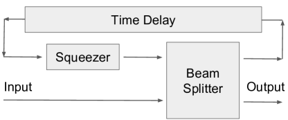
Figure 2. An example of a time-delay network in which enhanced squeezing occurs.

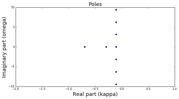
Figure 3. The poles of the transfer function of the example system

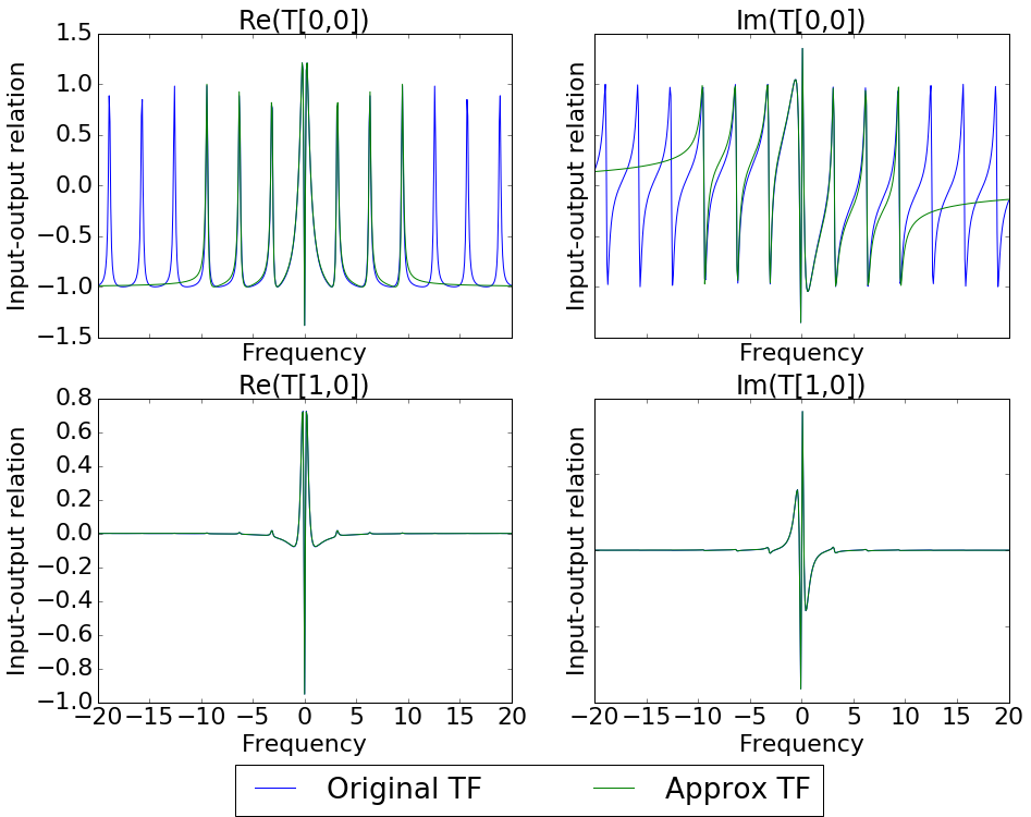
Figure 4. The transfer function of the example system, and the transfer function of an approximation generated using the canonical factors. A constant pre-factor was added so that the two functions match at the origin. The real and imaginary parts of two components are shown along $z=i\omega$ for real values of $\omega$.

10. Conclusion

We have shown how a factorization theorem can be obtained linear quantum network with delayed feedback under some stated assumptions. The conditions are fairly general, and allow for a wide class of quantum linear systems which may be active. The factorization generates a cascade of possibly infinitely many $2\times 2$ quantum linear systems, with transfer functions $P_{i}(z)$. These canonical terms can also include squeezing. Our theorem states that the factorization has form $\tilde{T}(z)=B\prod_{i}P_{i}(z)$, where $B$ is a constant matrix. We show that this product converges on compact sets. The $B$ matrix must be $J$-unitary and doubled-up as well.

One of our assumptions excludes cases with essentially feedforward delays, and other assumptions are made for simplicity. To get each individual factor, we also require non-degeneracy conditions to be met. However, as we showed in the example in Section 9, it is possible to find good approximations even when the non-degeneracy conditions are not met by perturbing the system.

11. Acknowledgements

GT is supported by an NDSEG fellowship awarded by the DoD and a Stanford University Graduate Fellowship. RH is supported by an appointment to the IC Postdoctoral Research Fellowship Program at MIT, administered by ORISE through U.S. DOE / ODNI. This work was also supported by ARO under grant “W911NF-16-1-0086.”

We would also like to thank discussions with Tatsuhiro Onodera, Nikolas Tezak, Hendra Nurdin, John E. Gough, Edwin Ng, Daniel B. Soh, Niels Lorch, and Eric Chatterjee.

Appendix A Proof of Lemma 6.3

remark A.1.

Because of the relationship we found between the zeros and poles for $J$-unitary functions (along with the eigenvectors at the zeros and poles), the lemma holds for the roots if and only if it holds for the poles. Therefore, it suffices to prove the lemma only for one or the other. We will prove parts (i) and (iii) of the theorem for the poles and part (ii) for the zeros.

proof for (i):

We begin by showing that for sufficiently large $M$, for each zero $w_{0}$ of $f_{S}(z)$ such that $|w_{0}|>M$, there is a radius $\epsilon_{M}=O(1/M)$ such that exactly one zero $z_{0}$ of $f_{T}(z)$ is within $\epsilon_{M}$ of $w_{0}$. To show this, we will use Rouché’s Theorem [17]. This theorem states that if $|f_{T}(z)-f_{S}(z)|<|f_{T}(z)|,|f_{S}(z)|$ for every $z$ on the boundary of some Jordan curve $\Gamma$, then $f_{T}(z)$ and $f_{S}(z)$ will have the same number of zeros in the interior of $\Gamma$.

We can ensure that for sufficiently large $M$, each $\epsilon_{M}$ is small enough so that it isolates a single zero $w_{0}$ of $f_{S}(z)$. To do this, first note that there is always a positive upper bound $\epsilon_{\text{max}}>0$ for the radii that isolate the zeros and poles of a not identically zero meromorphic function from other zeros and poles on a bounded set. Using the periodicity of $f_{S}(z)$ and the boundedness of the real part of the the zeros (Lemma 6.1), we can get the desired result. Given a relation $\epsilon_{M}=O(1/M)$ for sufficiently large $M$, we can make $\epsilon_{M}$ as small as we like (in particular we can satisfy $\epsilon_{M}<\epsilon_{\text{max}}$) by requiring $M$ to be sufficiently large.

In order to pick the bounds for Rouché’s theorem, we expand $f_{S}(z)$ at $w_{0}$. Explicitly, assuming that leading order terms have order one (see Remark A.2), we can expand:

(50) $$f_{S}(z)=c_{1}^{(S,w_{0})}(z-w_{0})+c_{2}^{(S,w_{0})}(z-w_{0})^{2}+...$$

There is an error bound $k^{(S,w_{0})}>0$ such that if $z\in B_{\epsilon}(w_{0})$, then

(51) $$|f_{S}(z)-c_{1}^{(S,w_{0})}(z-w_{0})|<k^{(S,w_{0})}\epsilon^{2}.$$

From this we obtain the bounds for $z$ on $\partial B_{\epsilon}(w_{0})$,

(52) $$|f_{S}(z)| >|c_{1}^{(S,w_{0})}|\epsilon-k^{(S,w_{0})}\epsilon^{2},$$

(53) $$|f_{T}(z)| >|c_{1}^{(S,w_{0})}|\epsilon-\delta_{M}-k^{(S,w_{0})}\epsilon^{2}.$$

Above in Eq. (53), we introduce $\delta_{M}=\sup_{\partial B_{\epsilon}(w_{0})}|f_{S}(z)-f_{T}(z)|$. Notice sufficient conditions for Rouché’s theorem are now $\delta_{M}<|f_{S}(z)|,|f_{T}(z)|$.

From Lemma 5.2, the poles of $\tilde{S}(z)$ are contained in a strip of bounded $\Re(z)$. This implies that there is a bound on the real part of all zeros of $f_{S}(z)$. Using Lemma 6.2 (ii), we can bound $\delta_{M}=O(1/M)$ for large enough $M$. We can also bound the coefficients $c_{1}^{(S,w_{0})}$ for all zeros $w_{0}$ of $f_{S}(z)$ from below by $C>0$. This follows from the periodicity of $f_{S}(z)$ in the imaginary direction, and noting that the bound on the real part of $z$ for the zeros of $f_{S}(z)$ implies that in each period there are a finite number of zeros. Similarly, we can bound all $k^{(S,w_{0})}$ from above by a constant $k$. If we pick $\epsilon_{M}=\frac{3\delta_{M}}{C}=O(1/M)$ for sufficiently large $M$, the desired conditions for Rouché’s theorem follow from the above inequalities.

For the case where $f_{S}(z)$ and $f_{T}(z)$ are exchanged, a small modification is needed to obtain the desired $\epsilon_{M}$, since $f_{T}(z)$ may not be periodic. First, we need to modify $\epsilon_{\text{max}}$ to ensure the poles $z_{0}$ are isolated. This can be done by an application of the triangle inequality. Next, we are interested in bounds for the constants $c_{1}^{(T,z_{0})}$ and $k^{(T,z_{0})}$ when expanding $f_{T}(z)$ at each of its zeros $z_{0}$, analogous to the constants used above in Eq. (50-51). Using Cauchy’s integral formula on the $\epsilon$-balls in the above arument, and the error estimate $|f_{T}(z)-f_{S}(z)|<\delta_{M}$, we can obtain the same bounds $C$ and $k$ above for the expansion coefficients $c_{i}^{(T,w_{0})}$ and $k^{(T,z_{0})}$, respectively, up to an error of $\delta_{M}=O(1/M)$. Therefore the desired result holds in this case as well. $\blacksquare$

proof for (ii):

Suppose we are given a pair of roots from part (i), $z_{0}$ for $f_{T}(z)$ and $w_{0}$ for $f_{S}(z)$, along with a radius $\epsilon_{M}$ such that $z_{0}$ is the only root of $f_{T}(z)$ and $w_{0}$ is the only root of $f_{S}(z)$ inside $B_{\epsilon_{M}}(w_{0})$. From $z_{0}$ and $w_{0}$ (which are poles of $\tilde{T}(z)$ and $\tilde{S}(z)$) we can find the corresponding roots of $\tilde{T}(z)$ and $\tilde{S}(z)$ (from Claim 5.5), which we label $\hat{z}_{0}$ and $\hat{w}_{0}$, respectively. Below we will consider all such possible pairs $\hat{z}_{0}$ and $\hat{w}_{0}$.

We will show first that

(54) $$\|\tilde{T}(\hat{z}_{0})-\tilde{S}(\hat{w}_{0})\|=O(\epsilon_{M}).$$

To do this, write

(55) $$\|\tilde{T}(\hat{z}_{0})-\tilde{S}(\hat{w}_{0})\|\leq\|\tilde{T}(\hat{z}_{0})-\tilde{S}(\hat{z}_{0})\|+\|\tilde{S}(\hat{z}_{0})-\tilde{S}(\hat{w}_{0})\|.$$

To find a bound for $\|\tilde{T}(\hat{z}_{0})-\tilde{S}(\hat{z}_{0})\|$ independent of the choice of $\hat{z}_{0}$ for sufficiently large $|z|$, we can use the bound $\kappa_{M}=\sup_{|z|>M}\|T_{i}(z)-S_{i}\|=O(1/M)$ for $i=1,2,3,4.$

We can bound

(56) $$\|\tilde{T}(z)-\tilde{S}(z)\|\leq\|T_{1}(z)-S_{1}\|$$

$$+\|T_{2}(z)-S_{2}\|\|E(z)\|\|(I-T_{4}(z)E(z))^{-1}-(I-S_{4}E(z))^{-1}\|\|T_{3}(z)-S_{3}\|$$

The $E(z)$ term is bounded for all $\hat{z}_{0}$, following Lemma 6.2 (ii). The term for which obtaining the bound is not obvious is $\|(I-T_{4}(z)E(z))^{-1}-(I-S_{4}E(z))^{-1}\|$. We do this below. When $|z|$ is sufficiently large, we can use Lemma 6.2 to write $T_{4}(z)=S_{4}+\nu_{\hat{w}_{0}}D_{\hat{w}_{0}}(z)$ on each $B_{\epsilon_{M}}(\hat{w}_{0})$ where all the functions $D_{\hat{w}_{0}}$ are bounded and matrix-valued, and $\nu_{\hat{w}_{0}}=O(1/|{\hat{w}_{0}}|)$. When $z\in B_{\epsilon_{M}}(\hat{w}_{0})$,

(57) $$(I-T_{4}(z)E(z))^{-1}$$

$$=(I-S_{4}E(z)-\nu_{\hat{w}_{0}}D_{\hat{w}_{0}}E(z))^{-1}$$

$$=(I-\nu_{\hat{w}_{0}}(I-S_{4}E(z))^{-1}D_{\hat{w}_{0}}E(z))^{-1}(I-S_{4}E(z))^{-1}$$

$$=(I+O(\nu_{\hat{w}_{0}}))^{-1}(I-S_{4}E(z))^{-1}.$$

In the final step of Eq. (57), we notice that since $\epsilon_{M}$ isolates the zero $\hat{w}_{0}$ from other zeros and poles of $\tilde{S}(z)$, the function $(I-S_{4}E(z))^{-1}$ is bounded on $B_{\epsilon_{M}}(\hat{w}_{0})$. From this we find

(58) $$(I-T_{4}(z)E(z))^{-1}-(I-S_{4}E(z))^{-1}$$

$$=[(I+O(\nu_{\hat{w}_{0}}))^{-1}-I](I-S_{4}E(z))^{-1}$$

$$=(I+O(\nu_{\hat{w}_{0}}))^{-1}O(\nu_{\hat{w}_{0}})(I-S_{4}E(z))^{-1}=O(\nu_{\hat{w}_{0}}).$$

Since $\hat{z}_{0}$ is in $B_{\epsilon_{M}}(\hat{w}_{0})$, This gives the desired bound

(59) $$\|\tilde{T}(\hat{z}_{0})-\tilde{S}(\hat{z}_{0})\|=O(1/M).$$

Further, by a periodicity argument similar to that in part (i), we can make the bound independent of the choice of zeros $\hat{z}_{0}$ and $\hat{w}_{0}$.

Next, we obtain a similar bound for $\|\tilde{S}(\hat{z}_{0})-\tilde{S}(\hat{w}_{0})\|$:

(60) $$\|\tilde{S}(\hat{z}_{0})-\tilde{S}(\hat{w}_{0})\|\leq\|S_{2}\|\|E(z)\|\|(I-S_{4}E(\hat{z}_{0}))^{-1}-(I-S_{4}E(\hat{w}_{0}))^{-1}\|\|S_{3}\|.$$

We notice that $\|E(\hat{z}_{0})-E(\hat{w}_{0})\|=O(\epsilon_{M})$, so using a similar argument as before,

(61) $$(I-S_{4}E(\hat{z}_{0}))^{-1}=(I-S_{4}E(\hat{w}_{0}))^{-1}(I+O(\epsilon_{M})).$$

We thus obtain

(62) $$\|\tilde{S}(\hat{z}_{0})-\tilde{S}(\hat{w}_{0})\|=O(1/M)$$

Using Eq. (59) and Eq. (62), we finally obtain Eq. (54).

Next, to relate our analysis to the projectors, we can use the formula [10]

(63) $$P=-\frac{1}{2\pi i}\int_{\Gamma}R(\zeta,A)d\zeta,$$

where $R(\zeta,A)=(A-\zeta)^{-1}$ is the resolvent of a matrix $A$, and $P$ is the sum of the eigenprojections of all the eigenvalues of $A$ inside the contour $\Gamma$.

We will use the second resolvent identity below. It states that for two matrices $A$ and $B$, and $\zeta$ a number not in the spectrum of either,

(64) $$R(\zeta,A)-R(\zeta,B)=R(\zeta,A)(B-A)R(\zeta,B).$$

In particular, since $\hat{z}_{0}$ and $\hat{w}_{0}$ are roots of $\tilde{T}(z)$ and $\tilde{S}(z)$, respectively, the matrices $\tilde{T}(\hat{z}_{0})$ and $\tilde{S}(\hat{w}_{0})$ both have the eigenvalue zero. For a sufficiently small contour $\Gamma$, the zero eigenvalue becomes isolated for both $\tilde{T}(\hat{z}_{0})$ and $\tilde{S}(\hat{w}_{0})$. The curve $\Gamma$ can be made a small, but fixed size for all $\hat{w}_{0}$ and $\hat{z}_{0}$. This will allow us to bound the resolvent $R$ below to be bound by a constant. From the second resolvent identity, we can obtain the bound:

(65) $$\|P_{T}-P_{S}\|\leq\frac{|\Gamma|}{2\pi}\sup_{\zeta\in\Gamma}R(\tilde{T}(\hat{z}_{0}),\zeta)\sup_{\zeta\in\Gamma}R(\tilde{S}(\hat{w}_{0}),\zeta)\|\tilde{T}(\hat{z}_{0})-\tilde{S}(\hat{w}_{0})\|=O(1/M).$$

Above, $|\Gamma|$ indicates the length of the curve $\Gamma$. The bound is independent of the choice of $\hat{w}_{0}$ and $\hat{z}_{0}$. This completes the proof.

$\blacksquare$

proof (iii) The proof follows the first step used to prove (ii), using the poles instead of the zeros. The boundedness of $(I-S_{4}E(z))^{-1}$ is obtained by the fixed bound $\epsilon$ away from the poles. $\blacksquare$

remark A.2.

Note on the rate of convergence: If the zeros have order $p$ instead of $1$, the scaling of $\epsilon_{M}$ follows $O(M^{-1/p})$. This can be seen from the order of the terms required in the series expansion used to prove part (i).

Appendix B Proof of Theorem 8.1

The roots come in conjugate pairs (Claim 5.7), so the set of roots can be partitioned into two conjugate sets: $Z=Z_{+}\cup Z_{-}$ where $Z_{-}=\{\overline{z}:z\in Z_{+}\}$. Since we assumed the delays are commensurate, the function $\tilde{S}(z)$ is periodic along the imaginary axis with some period $P$. Thus the roots in $Z_{+}$ (and $Z_{-}$) can be ordered as:

(66) $$Z_{+}=\Bigl{\{}\underbrace{z_{m}+iPn}_{z_{m,n}}:m\in\{1,...,M\},n\in\mathbb{Z}\Bigr{\}}$$

where $M$ is the number of roots (in $Z_{+}$) per period; because roots come in conjugate pairs, in total there are $2M$ roots per period. To satisfy the condition that all roots are simple (Assumption (6) of Section 4.1), we require that the $z_{n}$ be unique, satisfying $0<{\rm Im}(z_{m})<P$ and ${\rm Im}(z_{m})\neq P/2$. Thus all roots are complex, and a decomposition of the form (37) will be possible. We choose the ordering:

(67) $$\tilde{S}(z)=\Bigl{(}\prod_{m=1}^{K}\Bigl{[}\prod_{n=-\infty}^{\infty}P_{m,n}(z)\Bigr{]}\Bigr{)}B(z).$$

Here, $P_{m,n}(z)$ is the elementary factor with zeros $(z_{m,n},\overline{z}_{m,n})$ and poles $(-z_{m,n},-\overline{z}_{m,n})$ defined in Eq. (37).

We first show that each infinite product in Eq. (67) converges uniformly on bounded sets. Starting with $m=1$, consider the terms $P_{1,1},P_{1,2},\ldots$ generated by detaching the zeros $z_{1,1},z_{1,2},\ldots$ individually from $\tilde{S}(z)$. Since $\tilde{S}(z)$ is periodic with period $P$, so the projector of $\tilde{S}(z)$ at $z_{m,n}$ is independent of $n$. Thus the projectors in the terms used to detach the terms $P_{1,1},P_{1,2},\ldots$ are the same, and these terms commute. Therefore, these terms can be used to sequentially detach the roots of $\tilde{S}(z)$, giving the expression:

(68) $$\prod_{n}P_{m,n}(z) =I-V_{m}V_{m}^{\flat}+V_{m}\prod_{n}\begin{pmatrix}\frac{z-z_{m,n}}{z+\overline{z}_{m,n}}&0\\ 0&\left(\frac{\overline{z}-z_{m,n}}{\overline{z}+\overline{z}_{m,n}}\right)^{*}\end{pmatrix}V_{m}^{\flat}.$$

where we have fixed $m=1$ for the moment.

The above product converges because one can show [20, Appendix E] that the following series converges uniformly on bounded sets:

(69) $$Q_{m}(z) \equiv\prod_{n=-\infty}^{\infty}\frac{z-z_{m,n}}{z+\overline{z}_{m,n}}=\frac{\sinh\bigl{(}\frac{\pi}{P}(z-z_{m})\bigr{)}}{\sinh\bigl{(}\frac{\pi}{P}(z+\overline{z}_{m})\bigr{)}}$$

After the zeros $z_{1,1},z_{1,2},\ldots$ are detached, we obtain a function $\bigl{(}\prod_{i}P_{1,i}(z)\bigr{)}^{-1}\tilde{S}(z)$ which is again periodic in the imaginary direction with period $P$, but has only $2(M-1)$ zeros per period. We can repeat the same procedure for the remaining sequences of zeros $z_{m,1},z_{m,2},...$ in $Z_{+}$, finding:

(70) $$\tilde{S}(z)=\prod_{m=1}^{K}\biggl{[}1-V_{m}V_{m}^{\flat}+V_{m}\prod_{n}\begin{pmatrix}Q_{m}(z)&0\\ 0&Q_{m}(\overline{z})^{*}\end{pmatrix}V_{m}^{\flat}\biggr{]}B(z).$$

$B(z)$ is an entire function that, like $\tilde{S}(z)$ and $Q_{m}(z)$, is periodic along the imaginary axis with period $P$. In the limits ${\rm Re}(z)\rightarrow\pm\infty$, we can show that $B(z)$ tends to a constant by examining the behavior of $\tilde{S}(z)$ and $Q_{m}(z)$. For $\tilde{S}(z)$, recall that it is given by (32):

$$\tilde{S}(z) =S_{1}+S_{2}E(z)\left(I-S_{4}E(z)\right)^{-1}S_{3}$$

(71) $$=S_{1}+S_{2}\left(E(-z)-S_{4}\right)^{-1}S_{3}$$

Using the fact that $S_{4}$ is invertible and $E(z)\rightarrow 0$ for ${\rm Re}(z)\rightarrow+\infty$, it is easy to find the limiting behavior of $\tilde{S}(z)$. The limits of $Q_{m}(z)$ for ${\rm Re}(z)\rightarrow\pm\infty$ are found using (69) and the asymptotic relation $\sinh(x+iy)\rightarrow\tfrac{1}{2}{\rm sgn}(x)e^{|x|+iy\,{\rm sgn}(x)}$:

(72) $$\tilde{S}(z) \rightarrow\begin{dcases}S_{1}&{\rm Re}(z)\rightarrow+\infty\\ S_{1}-S_{2}S_{4}^{-1}S_{3}&{\rm Re}(z)\rightarrow-\infty\end{dcases},$$

(73) $$Q_{m}(z) \rightarrow\begin{dcases}e^{-(2\pi/P){\rm Re}(z_{m})}&{\rm Re}(z)\rightarrow+\infty\\ e^{+(2\pi/P){\rm Re}(z_{m})}&{\rm Re}(z)\rightarrow-\infty\end{dcases}.$$

These limits prove that $B(z)$ tends to a constant for $z\rightarrow\pm\infty$, when $\Im(z)$. We also know that $B(z)$ is periodic in the imaginary direction, since it is the product of commensurate periodic functions. Combining these two results, we determine that $B(z)$ has bounded range on the entire plane. By Liouville’s theorem, it must be a constant.

$\blacksquare$

Appendix C Proof of Theorem 8.2

The intuition for the proof of convergence will be to approximate the function $\tilde{T}(z)$ by $\tilde{S}(z)$ for large $|z|$ using Lemma 6.3.

From Lemma 6.3, we intuitively have that the zeros (poles) of $\tilde{T}(z)$ and $\tilde{S}(z)$ become arbitrarily close to one another as $|z|\to\infty$. Using this lemma, one can find a ball $B_{R_{0}}(0)$, with the following property: There is a one-to-one correspondence between the zeros (poles) of $\tilde{T}(z)$ and $\tilde{S}(z)$ outside $B_{R_{0}}(0)$, such that a zero (pole) $z_{0}$ of $\tilde{T}(z)$ and a zero (pole) $w_{0}$ of $\tilde{S}(z)$ correspond to each other if and only if $|z_{0}-w_{0}|<\epsilon_{R_{0}}=O(1/R_{0})$.

The order of terms being detached from $\tilde{T}(z)$ will be determined as follows. For terms with zeros inside $B_{R_{0}}(0)$, the order is not important for convergence, since there are a finite number of zeros inside $B_{R_{0}}(0)$. For example, we can pick the zeros according to increasing norm. For terms with zeros outside $B_{R_{0}}(0)$, the order is determined using the order of zeros of $\tilde{S}(z)$ in Theorem 8.1. That is, we use the one-to-one correspondence between the zeros of $\tilde{S}(z)$ and $\tilde{T}(z)$ to determine the order of zeros of $\tilde{T}(z)$. Detaching terms in this order gives $K$ (possibly) infinite products $\prod_{n}P_{m,n}$ for $m=1,...,K$, where $K$ is the number of zeros in each period of the zeros of $\tilde{S}(z)$ in Theorem 8.1. Our task is to show the products $\prod_{n}P_{m,n}$ converge for each $m$.

Consider one of the products $\prod_{n}P_{n}(z)$ (dropping the index m). Suppose the corresponding product generated for $\tilde{S}(z)$ by Theorem 8.1 is $\prod_{n}P_{n}^{S}(z)$. Here we do not include the terms with zeros inside $B_{R_{0}}(0)$. It will be convenient to use the form of the elementary factors introduced in Section 7.3. We can write

(74) $$P_{n}^{S}(z)=MF_{n}^{S}(z)M^{\dagger}J, F_{n}^{S}(z)=\text{diag}(a_{w_{n}}(z),-a_{w_{n}}(z^{*})^{*},1,-1,...,1,-1).$$

where $a_{z_{0}}(z)=\frac{z-z_{0}}{z+z_{0}^{*}}$ and $M$ is a fixed $J$-unitary. Here $w_{n}$ are the appropriate zeros of $\tilde{S}(z)$. Above in Eq. (74), M is fixed due to the periodicity argument used in Section 8.1. The terms $P_{n}(z)$ (with the zeros of $\tilde{T}(z)$) have form

(75) $$P_{n}(z) =\tilde{M}_{n}F_{n}(z)\tilde{M}_{n}^{\dagger}J,$$

(76) $$F_{n}(z) =\text{diag}(a_{z_{n}}(z),-a_{z_{n}}(z^{*})^{*},1,-1,...,1,-1).$$

Here ${z_{n}}$ are the appropriate zeros of $\tilde{T}(z)$, and $\tilde{M}={M+\epsilon_{R_{n}}N_{n}}$ is $J$-unitary. The $N_{n}$ are bounded matrices and $\epsilon_{R_{n}}=O(1/R_{n})$. In order to produce the $\tilde{M}_{n}$ related to $M$ by error $\epsilon_{R_{n}}$, apply Lemma 6.3(ii) to relate the $W$ matrices of $P_{n}$ and $P_{n}^{S}$ in the form of Eq. (43). In the remainder of the procedure of Section 7.3, we complete the basis of each to produce the respective $M$ matrices of Eq. (44). Care must be taken to ensure this procedure maintains the error bound for the $M$ matrices. For example, we can use Gram-Schmidt (with the indefinite basis), appending the same set of initial vectors in both cases.

Since we are interested in the convergence of $\prod_{n}P_{n}(z)$ on compact sets, fix $r>0$. We will show $\prod_{n}P_{n}(z)$ converges uniformly on $B_{r}(0)$. We will approximate $\prod_{n}P_{n}(z)$ on $B_{r}(0)$ using a sequence of functions $T_{\ell}(z)=\bigl{(}\prod_{n=\ell+1}^{\infty}P_{n}(z)\bigr{)}$ for $\ell=0,1,...$. Notice that $\prod_{n}P_{n}(z)=\left(\prod_{n=1}^{\ell}P_{n}(z)\right)T_{\ell}(z)$. Intuitively, we can think of the $T_{\ell}(z)$ as the truncation error. If the error can be controlled, then we can obtain a convergence result. Towards our goal we will show the following claim.

Claim C.1.

$T_{\ell}(z)$ converges uniformly on $B_{r}(0)$ as $\ell\to\infty$, using the supremum norm.

To prove the above claim, we will use our knowledge of $P_{n}(z)$ and $P_{n}^{S}(z)$ to show that for sufficiently large $R_{n}$, $\|P_{n}(z)-P_{n}^{S}(z)\|=O(1/R_{n}^{2})$ for $z\in B_{r}(z)$ where the zeros of $P_{n}(z)$ and $P_{n}^{S}(z)$ are outside $B_{R_{n}}(0)$. First, we show an estimate of the same order for $F_{n}(z)$ and $F_{n}^{S}(z)$:

(77) $$\|F_{n}(z)-F_{n}^{S}(z)\|\leq\|{F_{n}^{S}(z)}\|\|{F_{n}^{S}(z)}^{-1}F_{n}(z)-I\|$$

For large enough $R_{n}$, we can use $|a_{w_{n}}(z)-1|=O(1/R_{n})$ for $|w_{n}|>R_{n}$ to show

(78) $${F_{n}^{S}(z)}=J+O(1/R_{n}).$$

Here we use the rate of convergence result of Lemma 6.3. For estimating the term $\|{F_{n}^{S}(z)}^{-1}F_{n}(z)-I\|$, one can compute (using $\gamma_{n}=w_{n}-z_{n}=O(1/R_{n})$):

(79) $$a_{w_{n}}(z)a_{z_{n}}(z)^{-1} =\frac{z-w_{n}}{z+w_{n}^{*}}\frac{z+z_{n}^{*}}{z-z_{n}}=\frac{z-(z_{n}+\gamma_{n})}{z+(z_{n}+\gamma_{n})^{*}}\frac{z+z_{n}^{*}}{z-z_{n}}=\frac{1-\frac{\gamma_{n}}{z-z_{n}}}{1+\frac{\gamma_{n}^{*}}{z+z_{n}^{*}}}$$

$$=\left(1-\frac{\gamma_{n}}{z-z_{n}}\right)\left(1-\frac{\gamma_{n}^{*}}{z+z_{n}^{*}}\right)+O(|\gamma_{n}|^{2})$$

$$=1-\frac{\gamma_{n}}{z-z_{n}}-\frac{\gamma_{n}^{*}}{z+z_{n}^{*}}+O(|\gamma_{n}|^{2})$$

$$=1-\frac{\gamma_{n}}{z-w_{n}}-\frac{\gamma_{n}^{*}}{z+w_{n}^{*}}+O(|\gamma_{n}|^{2}).$$

For large enough $R_{n}$, the terms $(z-z_{n})^{-1}=O(1/R_{n})$ and $(z+z_{n}^{*})^{-1}=O(1/R_{n})$ since $|z_{n}|>R_{n}$. Thus we find

(80) $$a_{w_{n}}(z)a_{z_{n}}(z)^{-1} =1+O(|1/R_{n}^{2}|).$$

Using Eq. (78) and Eq. (80) in Eq. (77), we find

(81) $$\|F_{n}(z)-F_{n}^{S}(z)\|=(1+O(1/R_{n}))O(1/R_{n}^{2})=O(1/R_{n}^{2}).$$

We can then compute

$$\|P_{n}(z)-P_{n}^{S}(z)\| =\|(M+\epsilon_{R_{n}}N_{n})F_{n}(z)(M+\epsilon_{R_{n}}N_{n})^{\dagger}J-MF_{n}^{S}(z)M^{\dagger}J\|$$

$$=\|(M+\epsilon_{R_{n}}N_{n})F^{S}_{n}(z)(M+\epsilon_{R_{n}}N_{n})^{\dagger}J-MF_{n}^{S}(z)M^{\dagger}J\|+O(1/R^{2})$$

(82) $$=\epsilon_{R_{n}}\|N_{n}F^{S}_{n}(z)M^{\dagger}J+MF^{S}_{n}(z)N_{n}^{\dagger}J\|+O(1/R_{n}^{2}).$$

Using that $M$ and $M+\epsilon_{R_{n}}N_{n}$ are $J$-unitary, we find

(83) $$(M+\epsilon_{R_{n}}N_{n})J(M+\epsilon_{R_{n}}N_{n})^{\dagger}-MJM^{\dagger}=0,$$

from which we find

(84) $$N_{n}JM^{\dagger}+MJN_{n}^{\dagger}=O(1/R_{n}^{2}).$$

Using $F_{n}^{S}(z)=J+O(1/R_{n})$, Eq. (82), and Eq. (84), we find

(85) $$\|P_{n}(z)-P_{n}^{S}(z)\|=O(1/R_{n}^{2}).$$

This gives us a bound on the estimate error between $P_{n}(z)$ and $P_{n}^{S}(z)$ inside $B_{r}(0)$ for some sufficiently large $R_{n}$, which will be key in showing the convergence of $T_{\ell}(z)$. Notice that because the zeros $w_{n}$ of $\tilde{S}(z)$ are periodic, we can replace $O(1/R_{n}^{2})$ by $O(1/n^{2})$. Let $q$ be the smallest index of $n$ for which the above estimates Eqs. (78, 85) hold, and also that $R_{n}>r$.

The next step will be to show that $\|\prod_{n=q}^{p}P_{n}(z)\|$ is bounded in $B_{r}(0)$ for all $p=q,q+1,...$. Our estimate Eq. (85) produces

(86) $$\left\|\prod_{n=q}^{p}P_{n}(z)\right\|\leq\left\|\prod_{n=q}^{p}P_{n}^{S}(z)\right\|\prod_{n=q}^{p}\left(1+\frac{c}{n^{2}\|P_{n}^{S}(z)\|}\right).$$

The product $\prod_{n=q}^{p}P_{n}^{S}(z)$ is bounded on $B_{r}(0)$ over all $p=q,q+1,...$ since it converges in the limit $p\to\infty$, and it has no poles in $B_{r}(0)$ (since we ensured $R_{n}>r$). Also, $\|P_{n}^{S}(z)\|$ converges to a constant as $n\to\infty$ because $a_{w_{n}}(z)\to 1$ as $|w_{n}|\to\infty$. Finally we can obtain a bound for Eq. (86) over all $p=q,q+1,...$ since $\sum_{n=1}^{\infty}\frac{1}{n^{2}}$ converges.

Next, we are ready to show the sequence of functions $T_{\ell}(z)$ is Cauchy with the supremum norm on $B_{r}(0)$. To see this, we can compute for $z\in B_{r}(0)$ and $q\leq\ell<k$,

(87) $$\|T_{\ell}(z)-T_{k}(z)\|\leq\left\|\prod_{n=q}^{\ell}P_{n}(z)\right\|\left\|\prod_{n=\ell+1}^{k}(P_{n}(z)-P_{n}^{S}(z))\right\|\left\|\prod_{k+1}^{\infty}P_{n}^{S}(z)\right\|.$$

We have shown the first term is bounded over all $\ell=q,q+1,...$, and the last term is bounded as discussed above. The middle term can be made arbitrarily small for sufficiently large $\ell$ and $k$ using the bound in Eq. (85). We conclude from this that $T_{\ell}(z)$ is uniformly Cauchy on $B_{r}(0)$, and therefore converges uniformly. This completes the proof of Claim C.1.

Finally, we can show $\prod_{n=q}^{\infty}P_{n}(z)=\left(\prod_{n=q}^{\ell}P_{n}(z)\right)T_{\ell}(z)$ converges uniformly on $B_{r}(0)$ using the uniform convergence of $T_{\ell}(z)$ and the upper bound Eq. (86). Explicitly, supposing $C(z)$ is the function satisfying $T_{\ell}(z)\to C(z)$ as $\ell\to\infty$ uniformly on $B_{r}(0)$, we find

(88) $$\left\|\prod_{n=q}^{\infty}P_{n}(z)-\left(\prod_{n=q}^{\ell}P_{n}(z)\right)C(z)\right\|\leq\left\|\prod_{n=q}^{\ell}P_{n}(z)\right\|\|C(z)-T_{\ell}(z)\|.$$

Since $q$ was just a finite integer, we conclude that $\prod_{n}P_{n}(z)$ converges uniformly on $B_{r}(0)$.

Finally, to complete the proof of Theorem 8.2, we wish to show $B(z)$ is a constant. To do this, it suffices to show it is a bounded function, since it is entire (using Liouville’s theorem). Since $\tilde{T}(z)$ is not periodic like $\tilde{S}(z)$, we cannot use the same proof as for Theorem 8.1. We have $B(z)=\bigl{(}\prod_{n}P_{n}(z)\bigr{)}^{-1}\tilde{T}(z)$, and let $B_{S}(z)=\bigl{(}\prod_{n}P^{S}_{n}(z)\bigr{)}^{-1}\tilde{S}(z)$. Since $B_{S}=B_{S}(z)$ is constant as found in Theorem 8.1, it suffices to show $\|B_{S}-B_{T}(z)\|$ is bounded regardless of $z$.

We apply part (iii) of Lemma 6.3, in order to approximate $\tilde{T}(z)$ with $\tilde{S}(z)$ away from their poles $z_{n}$ and $w_{n}$. For a small but fixed $\epsilon$ and sufficiently large $M$, if $|z|>M$ and $z\notin B_{\epsilon}(w_{n})$, $z\notin B_{\epsilon}(z_{n})$

(89) $$\|\tilde{T}(z)-\tilde{S}(z)\|=O(1/M).$$

We will next find an estimate for $\|\bigl{(}\prod_{n}P_{n}(z)\bigr{)}^{-1}-\bigl{(}\prod^{S}_{n}P_{n}(z)\bigr{)}^{-1}\|$ for sufficiently large $|z|$ and $z\notin B_{\epsilon}(w_{n}),z\notin B_{\epsilon}(z_{n})$, using the bounds found above. We will show the proof for $\|\prod_{n}P_{n}(z)-\prod^{S}_{n}P_{n}(z)\|$ to simplify the notation, since each $P_{n}(z)$ has the same form as $P_{n}(z)^{-1}$ (same for $P_{n}^{S}(z))$. To do this, we will start with the estimate Eq. (79). The terms $(z-w_{n})^{-1}$ and $(z+w_{n}^{*})^{-1}$ can be uniformly bounded if we ensure that $z$ is at least $\epsilon$ away from each $w_{n}$, $-w_{n}^{*}$. However, now we cannot bound these terms by $O(1/R_{n})$ since $z$ is not confined to $B_{r}(0)$. Instead we can propagate error terms of the form $O(1/|z-w_{n}|)$ and $O(1/|z+w_{n}^{*}|)$ through the analysis, obtaining an estimate similar to Eq. (85),

(90) $$\|P_{n}(z)-P_{n}^{S}(z)\| =O(1/R_{n}^{2})+O(1/(R_{n}|z-w_{n}|))+O(1/(R_{n}|z+w_{n}^{*}|)).$$

which holds when $|w_{n}|,|z_{n}|>R_{n}$ for sufficiently large $R_{n}$.

We can continue similarly to Eq. (86), finding a sufficiently large index $q$ so that

(91) $$\left\|\prod_{n=q}^{\infty}P_{n}(z)\right\|\leq\left\|\prod_{n=q}^{\infty}P^{S}_{n}(z)\right\|\prod_{n=q}^{\infty}\left(1+c\left(\frac{1}{n^{2}}+\frac{1}{n^{2}|z/w_{n}-1|}+\frac{1}{n^{2}|z/w_{n}^{*}+1|}\right)\frac{1}{\|P_{n}^{S}(z)\|}\right),$$

for a constant $c$. Next we examine individual terms above in Eq. (91) and check they are all bounded uniformly when $z\notin B_{\epsilon}(w_{n}),z\notin B_{\epsilon}(-w_{n}^{*})$. In this domain we can obtain a bound for $\left\|\prod_{n=q}^{\infty}P^{S}_{n}(z)\right\|$ (which depends on our choice of $\epsilon$). This can be done by considering $\prod_{n=1}^{\infty}P^{S}_{n}(z),$ which is periodic in the imaginary direction. The product also converges as $\Re(z)\to\pm\infty$, so we conclude $\left\|\prod_{n=q}^{\infty}P^{S}_{n}(z)\right\|$ is bounded uniformly for $z\notin B_{\epsilon}(w_{n}),z\notin B_{\epsilon}(z_{n})$. We also have $\|P_{n}^{S}(z)\|$ are uniformly bounded away from zero when $z\notin B_{\epsilon}(w_{n}),z\notin B_{\epsilon}(-w_{n}^{*})$. As before, $\sum_{n=1}^{\infty}\frac{1}{n^{2}}$ converges. The terms $\sum_{n=1}^{\infty}\frac{1}{n^{2}|z/w_{n}-1|}$ and $\sum_{n=1}^{\infty}\frac{1}{n^{2}|z/w_{n}^{*}+1|}$ are bounded uniformly when $z$ is bounded away by the fixed $\epsilon$ away from $w_{n}$ (and $-w_{n}^{*}$). We can combine these observations to show that $\left\|\prod_{n}P_{n}(z)-\prod_{n}P_{n}^{S}(z)\right\|$ is bounded as long as $z\notin B_{\epsilon}(w_{n}),z\notin B_{\epsilon}(z_{n})$ (further, the same holds for $\|\left(\prod_{n}P_{n}(z)\right)^{-1}-\left(\prod_{n}P_{n}^{S}(z)\right)^{-1}\|$). With the same conditions on $z$, since $\prod_{n}P^{S}_{n}(z)$ is also bounded, we find that $\prod_{n}P_{n}(z)$ is bounded as well.

Combining the above result with Eq. (89), and the boundedness of $\tilde{S}(z)$, we find that for sufficiently large $|z|$ for which $z\notin B_{\epsilon}(w_{n}),z\notin B_{\epsilon}(-w_{n}^{*}),z\notin B_{\epsilon}(z_{n})$,

$$\|B(z)-B_{S}(z)\|$$

(92) $$\leq\biggl{\|}\Bigl{(}\prod_{n}P_{n}(z)\Bigr{)}^{-1}\biggr{\|}\left\|\tilde{T}(z)-\tilde{S}(z)\right\|+\left\|\tilde{S}(z)\right\|\biggl{\|}\Bigl{(}\prod_{n}P_{n}(z)\Bigr{)}^{-1}-\Bigl{(}\prod_{n}P^{S}_{n}(z)\Bigr{)}^{-1}\biggr{\|}.$$

Since we can make $\epsilon$ as small as we wish, we can ensure it is small enough so that there is a sequence of discs $B_{r_{n}}(0)$ with $r_{n}\to\infty$ as $n\to\infty$ such that none of the boundaries $\partial B_{r_{n}}(0)$ contain points in any of the $\epsilon$ neighborhoods of the balls $B_{\epsilon}(w_{n}),B_{\epsilon}(-w_{n}^{*}),B_{\epsilon}(z_{n})$. By the maximum modulus principle, the maximum value of $\|B(z)\|$ on each $B_{r_{n}}(0)$ is attained on the boundary. Further, this value is bounded independently of $z$. This implies $B(z)$ is everywhere bounded, and hence a constant (call it $B$). $\blacksquare$

References

- [1] Joshua Combes, Joseph Kerckhoff, and Mohan Sarovar. The SLH framework for modeling quantum input-output networks. Advances in Physics: X, 2(3):784–888, 2017.
- [2] Orion Crisafulli, Nikolas Tezak, Daniel BS Soh, Michael A Armen, and Hideo Mabuchi. Squeezed light in an optical parametric oscillator network with coherent feedback quantum control. Optics Express, 21(15):18371–18386, 2013.
- [3] Israel Gohberg, Peter Lancaster, and Leiba Rodman. Indefinite Linear Algebra and Applications. Springer Science & Business Media, 2006.
- [4] John E Gough, Symeon Grivopoulos, and Ian R Petersen. Isolated loops in quantum feedback networks. arXiv preprint arXiv:1705.09916, 2017.
- [5] John Edward Gough, MR James, and HI Nurdin. Squeezing components in linear quantum feedback networks. Physical Review A, 81(2):023804, 2010.
- [6] John Edward Gough and Sebastian Wildfeuer. Enhancement of field squeezing using coherent feedback. Physical Review A, 80(4):042107, 2009.
- [7] Arne L Grimsmo. Time-delayed quantum feedback control. Physical Review Letters, 115(6):060402, 2015.
- [8] Symeon Grivopoulos, Hendra I Nurdin, and Ian R Petersen. On transfer function realizations for linear quantum stochastic systems. In Decision and Control (CDC), 2016 IEEE 55th Conference on, pages 4552–4558. IEEE, 2016.
- [9] Sanae Iida, Mitsuyoshi Yukawa, Hidehiro Yonezawa, Naoki Yamamoto, and Akira Furusawa. Experimental demonstration of coherent feedback control on optical field squeezing. IEEE Transactions on Automatic Control, 57(8):2045–2050, 2012.
- [10] T Kato. Perturbation Theory for Linear Operators, volume 132. W. Springer-Verlag Berlin, 1976.
- [11] Manuel Kraft, Sven M Hein, Judith Lehnert, Eckehard Schöll, Stephen Hughes, and Andreas Knorr. Time-delayed quantum coherent pyragas feedback control of photon squeezing in a degenerate parametric oscillator. Physical Review A, 94(2):023806, 2016.
- [12] Sanjay Lall. Lecture notes on state-space realization theory. http://lall.stanford.edu/svn/engr207c_2010_to_2011_autumn/data/realization_2008_11_15_03.pdf, November 2008. Accessed: May 24 2017.
- [13] Nikolett Német and Scott Parkins. Enhanced optical squeezing from a degenerate parametric amplifier via time-delayed coherent feedback. Physical Review A, 94(2):023809, 2016.
- [14] Hendra I Nurdin, Symeon Grivopoulos, and Ian R Petersen. The transfer function of generic linear quantum stochastic systems has a pure cascade realization. Automatica, 69:324–333, 2016.
- [15] Hannes Pichler and Peter Zoller. Photonic circuits with time delays and quantum feedback. Physical review letters, 116(9):093601, 2016.
- [16] Carl L Prather and André C M Ran. Factorization of a class of meromorphic matrix valued functions. Journal of Mathematical Analysis and Applications, 127(2):413–422, 1987.
- [17] Edward B Saff and Arthur David Snider. Fundamentals of Complex Analysis for Mathematics, Science, and Engineering. Prentice-Hall, 1976.
- [18] AJ Shaiju and Ian R Petersen. A frequency domain condition for the physical realizability of linear quantum systems. IEEE Transactions on Automatic Control, 57(8):2033–2044, 2012.
- [19] Gil Tabak. Example for factorizing quantum linear systems with time delays. https://github.com/tabakg/active_lin_sys_fact/blob/master/sample_active_linear_system_3.ipynb, February 2018.
- [20] Gil Tabak and Hideo Mabuchi. Trapped modes in linear quantum stochastic networks with delays. EPJ Quantum Technology, 3(1):3, 2016.
- [21] SJ Whalen, AL Grimsmo, and HJ Carmichael. Open quantum systems with delayed coherent feedback. Quantum Science and Technology, 2(4):044008, 2017.