Learning-based Dequantization for Image Restoration Against Extremely Poor Illumination

Abstract

All existing image enhancement methods, such as HDR tone mapping, cannot recover A/D quantization losses due to insufficient or excessive lighting, (underflow and overflow problems). The loss of image details due to A/D quantization is complete and it cannot be recovered by traditional image processing methods, but the modern data-driven machine learning approach offers a much needed cure to the problem. In this work we propose a novel approach to restore and enhance images acquired in low and uneven lighting. First, the ill illumination is algorithmically compensated by emulating the effects of artificial supplementary lighting. Then a DCNN trained using only synthetic data recovers the missing detail caused by quantization.

1 Introduction

Photographs taken in dark environments or in poor uneven illumination conditions, such as in the night or backlighting, often become illegible due to low intensity, much compressed dynamic range, low contrast, and excessive noises. Nowadays, even mass-marketed digital cameras use high-resolution sensors and large capacity memory, unsatisfactory spatial resolutions and compression artifacts are not problems anymore. But extremely poor lighting, which is beyond users’ control and defies autoexposure mechanism, remains a common, uncorrected and yet understudied cause of image quality degradation.

The direct consequence of poor lighting is much compressed dynamic range of the acquired image signal. Existing image enhancement methods can expand the dynamic range via tone mapping, but they are inept to recover quality losses due to the A/D quantization of low amplitude signals. As a result, the tone-mapped images may appear sufficiently bright with good contrast, but finer details are completely erased.

As the non-linear quantization operation is not invertible, the image details erased by the A/D converter, when operating on weak and low dynamic range image signals, cannot be recovered by traditional image processing methods, such as high-pass filtering. The technical challenge in dequantizing images of compressed dynamic range is how to estimate and compensate for the quantization distortions. Up to now little has been done on the above missing data problem of A/D dequantization, leaving consumers’ long desire for low light cameras unsatisfied.

In this work we propose a novel approach to restore and enhance images acquired in low and uneven lighting. First, the ill illumination is algorithmically compensated by emulating the effects of artificial supplementary lighting based on an image formation model. The soft light compensation is only an initial step to increase the overall intensity and expand the dynamic range. It is not equivalent to photographing using flash, for the quantization losses incurred in the A/D conversion of low dynamic range images cannot be recovered in this way. Therefore, a subsequent step of the A/D dequantization is required, and this task is particularly suited for the methodology of deep learning, as will be demonstrated by this research.

Deep convolutional neural networks (DCNN) have been recently proven highly successful in image restoration tasks, including superresolution, denoising and inpainting. But as the loss of information due to quantization of low dynamic range images is not in the spatial but pixel value domain, machine learning based A/D dequantization appears to be more difficult than aforementioned other problems of image restoration, and warrants some closer scrutiny.

As in all machine learning methods, the performance of the learnt dequantization neural network primarily depends the quantity and quality of the training data. Using the same physical image formation model for light compensation, we derive an algorithm to generate training images of compressed dynamic range, by degrading corresponding latent images of normal dynamic range (ground truth for supervised learning). The artifacts of the training images closely mimic those caused by poor lighting conditions in real camera shooting. In addition to the good data quality, the generation algorithm is designed in such a way that it can take ubiquitous, widely available JPEG images as input, thus the machine learning for the A/D dequantization task can benefit from practically unlimited amount of training data.

2 Related work

As one of the fundamental problem in computer vision and image processing, image enhancement has been widely used as a key step in many applications such as image classification [1, 2], image recognition [3, 4], and object tracking [5]. Many popular enhancement methods are based on histogram equalization [6, 7]. These methods generally map the tone of the input image globally while ignoring the relationship of pixels with their neighbors. Variational methods try to resolve this problem by imposing different regularization terms based on different local features. For instance, contextual and variational contrast enhacement (CVC) [8] finds the histogram mapping to get large gray-level difference, while the method by Lee et al. [9] enhances image by amplifying the gray-level differences between adjacent pixels based on the layered difference representation of 2D histogram. Further more, optical tone mapping (OCTM) [10] was introduced for image enhancement via optimal contrast-tone mapping. Its variation [11] optimizes for maximal contrast gain while preserving the hue component.

Another popular family of image enhancement algorithms is based on the retinex theory, which explains the color and luminance perception property of human vision system [12]. The most important assumption of retinex theory is that an image can be decomposed to illumination and reflectance. Based on this idea, single-scale retinex (SSR) [13] is designed to estimate the reflectance and output it as an enhanced image. Multi-scale retinex (MSR) [14] extends retinex algorithm using multiple versions of the image on different scales. Both SSR and MSR assume that the illumination image is spatially smooth, which might not be true in real-world scenarios, as a result, the output of these techniques often look unnatural in unevenly illuminated regions. LIME [15] achieves good result by imposing a structure prior on the illumination map. SRIE [16] employs a weighted variational model to estimate both the reflectance and the illumination, and apply this model in manipulating the illumination map. Based on the observation that an inverted low-light image look like an image with haze, dehaze techniques are also used for low-light image enhancement  [17, 18]. The work in [19] is based on statistical modelling of wavelet coefficients of the image.

Most existing low-light image enhancement techniques are model-based rather than data-driven. A recent neural network based attempt is made to identify signal features from lowlight images and brighten images adaptively without over-amplifying or saturating the lighter parts in images with a high dynamic range [20]. However, this technique only alleviates the uneven illumination, leaving the problem of quantization unsolved.

3 Preparation of Training Data

The proposed technique reduces the quantization artifacts of a enhanced low-light image by using image details learned from other natural images. The effectiveness of our technique, or any machine learning approaches, greatly relies on the availability of a representative and sufficiently large set of training data. In this section, we discuss the methods for collecting and preparing the training images for our technique.

To help the proposed technique identify the quantization artifacts caused by poor illumination in real-world scenarios, ideally, the training algorithm should only use real photographs as the training data. Obtaining a pair of low-light and normal images is easy; we can take two consecutive shots of the same scene using different camera exposure settings. However, it is not easy to keep the pair of images perfectly aligned, especially when the imaged subject, such as a human, is in motion. Another possible solution is to synthesize two images of different brightness from a high dynamic range raw image by simulating all the digital processes in a camera from demosaicing to gamma correction to compression. While image alignment is not a concern using this method, collecting a large number of raw images of various scenes is still a difficult and costly task.

In this research, we employ a simple data synthesis approach that constructs realistic low-light images directly from normal low dynamic range images. As this approach does not require the original image to be raw or high dynamic range, a huge number of images covering various types of scenes are readily available online for training the purposed technique. To show how the data synthesis approach works, we first assume that the formation of an image $I$ on camera can be modelled as the piece-wise product of the illumination image $L$ and the reflectance image $R$, as follows,

$$I(i)=L(i)R(i),$$ (1)

for a pixel at location $i$.

By the image formation model, if the illumination of the captured scene decreases uniformly from $L$ to $aL$ by a factor of $a$ where $a<1$, then the captured image becomes attenuated to $aI$. However, if an input image $J$ is in JPEG format, as do the majority images available online, $J$ must have been gamma corrected and quantized, i.e.,

$$J(i)=Q([I(i)]^{\gamma_{1}}),$$ (2)

where $\gamma_{1}$ is the gamma correction coefficient and

$$Q(x)=q\cdot\lfloor x/q+0.5\rfloor,$$ (3)

is a quantization operator for some constant $q$. As image $J$ is not linear to the raw sensor reading $I$, simply multiplying $J$ by $a$ does not yield an accurate approximation of the corresponding low-light image with light being dimmed by factor $a$. Moreover, the true sensor reading $I$ cannot be recovered by using inverse gamma correction, as the gamma correction coefficient $\gamma_{1}$ is likely unknown for image $J$ collected online.

Suppose $J_{a}$ is a JPEG image captured under dimmed light with factor $a$, then by the definition of $I$ and $J$ in Eqs. (1) and (2),

$$J_{a}(i) =Q([aL(i)R(i)]^{\gamma_{2}}),$$

$$=Q(a^{\gamma_{2}}[I(i)]^{\gamma_{2}}),$$ (4)

where $\gamma_{2}$ is the gamma correction coefficient for the low-light image, which is not necessarily the same as $\gamma_{1}$. Since $J(i)$ is a quantized version of $[I(i)]^{\gamma_{1}}$ as defined in Eq. (2),

$$J(i)=[I(i)]^{\gamma_{1}}+n_{Q}(i),$$ (5)

where $n_{Q}(i)$ is the quantization noise. Therefore, $J_{a}(i)$ can be formulated as a function of $J(i)$, as follows,

$$J_{a}(i) =Q(a^{\gamma_{2}}[J(i)-n_{Q}(i)]^{\gamma_{2}/\gamma_{1}})$$

$$=Q(a^{\gamma_{2}}[J(i)]^{\gamma_{2}/\gamma_{1}})+n(i),$$ (6)

where term $n(i)$ accounts for the overall effects of $n_{Q}$ after being gamma transformed and requantized.

Effectively, the low-light image $J_{a}$ is a gamma-corrected, dyanmic range compressed and then quantized version of image $J$, as modelled in Eq. (6). By reverting the dynamic range compression and gamma correction applied on $J_{a}$, we get a degraded image $\tilde{J}$ with correct exposure but tainted with realistic quantization artifacts,

$$\tilde{J}(i) =\left(\frac{J_{a}(i)}{a^{\gamma_{2}}}\right)^{\gamma_{1}/\gamma_{2}}.$$ (7)

This is the way to generate a large, high-quality training data set $\mathcal{T}$ to facilitate the deep learning method to be introduced next.

4 Quasi-$\ell_{\infty}$ Dequantization with Generative Adversary Neural Networks

4.1 Design Objective

In order to solve the A/D dequantization problem, the standard method of deep learning is to train a deep convolutional neural network $G$ that minimizes a loss function $L_{G}$, that is,

$$G=\mathop{\arg\min}_{G}\sum_{(J,\tilde{J})\in\mathcal{T}}L_{G}(J,G(\tilde{J})),$$ (8)

where $(J,\tilde{J})$ is a sample pair drawn from $\mathcal{T}$ and accordingly $\hat{J}=G(\tilde{J})$ is the input-output mapping of network $G$.

But our problem has its unique characteristics, which need to be reflected by the loss function $L_{G}$. First, the training image pairs $(J,\tilde{J})\in\mathcal{T}$ have a very high level of variability, because we need to generate $\tilde{J}$ over a sufficiently large range of $a^{\gamma_{2}}$, $\gamma_{2}/\gamma_{1}$, and $n$. This is necessary if the trained network $G$ is to avoid the risk of data over fitting and perform robustly in all poor lighting conditions and camera settings. However, the spatial structures of quantization residuals, which is the very information to be recovered by deep learning, are largely independent of the lighting level $a$ and parameters $\gamma_{1}$ and $\gamma_{2}$. Therefore, we can greatly reduce the variability of the outputs of $G$ and thus improve the performance of the network, by changing the variables of the loss function $L_{G}$:

$$G=\mathop{\arg\min}_{G}\sum_{(J,\tilde{J})\in\mathcal{T}}L_{G}(J-\tilde{J},G(\tilde{J})).$$ (9)

In other words, network $G$ learns to predict, from $\tilde{J}$, the quantization residual,

$$E(\tilde{J})=J-\tilde{J},$$ (10)

rather than the latent image $J$ directly.

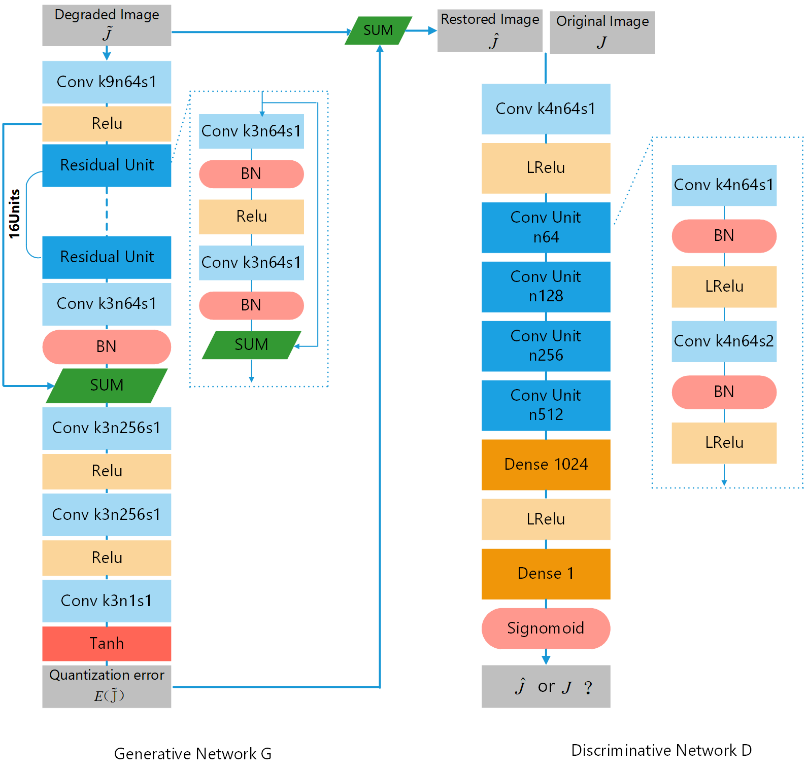
Fig. 1: The architecture of the proposed generative and adversarial networks.

4.2 GAN Construction

The next critical design decision is what are suitable quality criteria for the reconstructed image $\hat{J}$, which is to guide the construction of network $G$. For most users, the goals of enhancing poorly exposed images are overall legibility and aesthetics; signal level precision is secondary. This image quality preference is exactly the strength of the adversarial neural networks (GAN). In GAN, two neural networks, one called the generative network $G$ and the other the discriminative network $D$, contest against each other. In our case, network $G$ is the one stated in Eq. (9). It strives to generate an image $G(\tilde{J})$ to past the test of being a properly exposed image $J$ that is conducted by network $D$. On the other hand, network $D$ is trained to discriminate and reject the output images of network $G$.

The two competing networks $G$ and $D$ are constructed as shown in Fig. 1. The image $\tilde{J}$ of poor exposure and compressed dynamic range is fed into the generative network $G$ to be repaired. Network $G$ is trained to predict the quantization residual. Adding this residual to input image $\tilde{J}$ yields a restored image $\hat{J}$. Then, the restored image $\hat{J}$ and the latent image $J$ are used to train the discriminative network $D$. Reciprocally, network $D$ outputs its discriminator result of $\tilde{J}$ to help train network $G$.

As illustrated in Fig. 1, network $G$ is constructed as a deep convolution neural network, to exploit its ability to learn a mapping of high complexity. Our network $G$ contains 16 residual units [3], each consisting of two convolutional layers, two batch normalization layers [21] and one ReLU activation layers. For the architecture of network $D$, we borrowed the design of DCGAN [22]. It has four convolution units, each of which has two convolution layers, one with stride 1 and the other with stride 2. They are respectively followed by one batch normalization layer and one leakyRelu activation layer ($\alpha=0.2$) [23].

The output of the discriminative network, $D(\hat{J})$ or $D(J)$, can be interpreted as the probability that the underlying image is acquired in proper illumination conditions.

Following the idea of Goodfellow et al., we set a discriminative network $D$, which is optimized in conjunction with $G$, to solve the following min-max problem:

$$\min_{G}\max_{D}\left\{\mathbb{E}_{J}\big{[}\log D(J)\big{]}+\mathbb{E}_{\hat{J}}\big{[}\log(1-D(G(\hat{J})))\big{]}\right\}$$ (11)

In practice, for better gradient behavior, we minimize $-\log D(G(\hat{J}))$ instead of $\log(1-D(G(\hat{J})))$, as proposed in [24]. This introduces an adversarial term in the loss function of the generator CNN $G$:

$$L_{\oslash}=-\log D(G(\hat{J})).$$ (12)

In competition against generator network $G$, the loss function for training discriminative network $D$ is the binary cross entropy:

$$L_{D}=-\big{[}\log(D(J))+\log(1-D(G(\hat{J})))\big{]}$$ (13)

Minimizing $L_{\oslash}$ drives network $G$ to produce restored images that network $D$ cannot distinguish from properly exposed images. Accompanying the evolution of $G$, minimizing $L_{D}$ increases the discrimination power of network $D$.

4.3 Quasi-$\ell_{\infty}$ Loss

As observed in  [25] [26], adversarial training will drive the reconstruction towards the natural image manifold, producing perceptually agreeable results. However, the generated images are prone to fabricated structures that deviate too much from the ground truth. Particularly in our case, the learnt quantization residuals are to be added onto a base layer image. If these added structures are unrestricted at all, they could cause undesired artifacts, such as halos. To overcome these weaknesses of adversarial training, we introduce a structure-preserving quasi-$\ell_{\infty}$ loss term $L_{\infty}$ to tighten up the signal-level slack of probability divergence loss terms $L_{D}$ and $L_{\oslash}$.

To construct the loss term $L_{\infty}$, we first show that the restored image should be bounded by the degraded image $\tilde{J}$. By the definitions of $\tilde{J}$ in Eq. (7) and the low-light image $J_{a}$ in Eq. (6), we have,

$$Q(a^{\gamma_{2}}[J(i)]^{\gamma_{2}/\gamma_{1}})+n(i) =a^{\gamma_{2}}[\tilde{J}(i)]^{\gamma_{2}/\gamma_{1}}.$$ (14)

Then, by the definition of the quantization operator $Q(x)$ in Eq. (3),

$$\left|a^{\gamma_{2}}[\tilde{J}(i)]^{\gamma_{2}/\gamma_{1}}-n(i)-a^{\gamma_{2}}[J(i)]^{\gamma_{2}/\gamma_{1}}\right| \leq\frac{q}{2}.$$ (15)

To enforce these inequalities in the proposed neural network, we employ a barrier function in the quasi-$l^{\infty}$ loss function $L_{\infty}$ as follows,

$$L_{\infty}=\sum_{i\in B}-\log\left(1-\max\left\{|C(i)|-\frac{q}{2},0\right\}\right),$$ (16)

where $B$ is the pixel patch used in the training and,

$$C(i)=a^{\gamma_{2}}[\tilde{J}(i)]^{\gamma_{2}/\gamma_{1}}-a^{\gamma_{2}}[\hat{J}(i)]^{\gamma_{2}/\gamma_{1}}-n(i).$$ (17)

Plotted in Fig. 2 is the quasi-$l^{\infty}$ loss function. As shown in the figure, the quasi-$\ell_{\infty}$ loss is 0 within the quantization interval, and it increases rapidly once the pixel value falls outside of the interval.

Finally, we combine the adversarial loss and quasi-$\ell_{\infty}$ loss when optimizing the generative network $G$, namely,

$$L_{G}=L_{\infty}+\lambda L_{\oslash}.$$ (18)

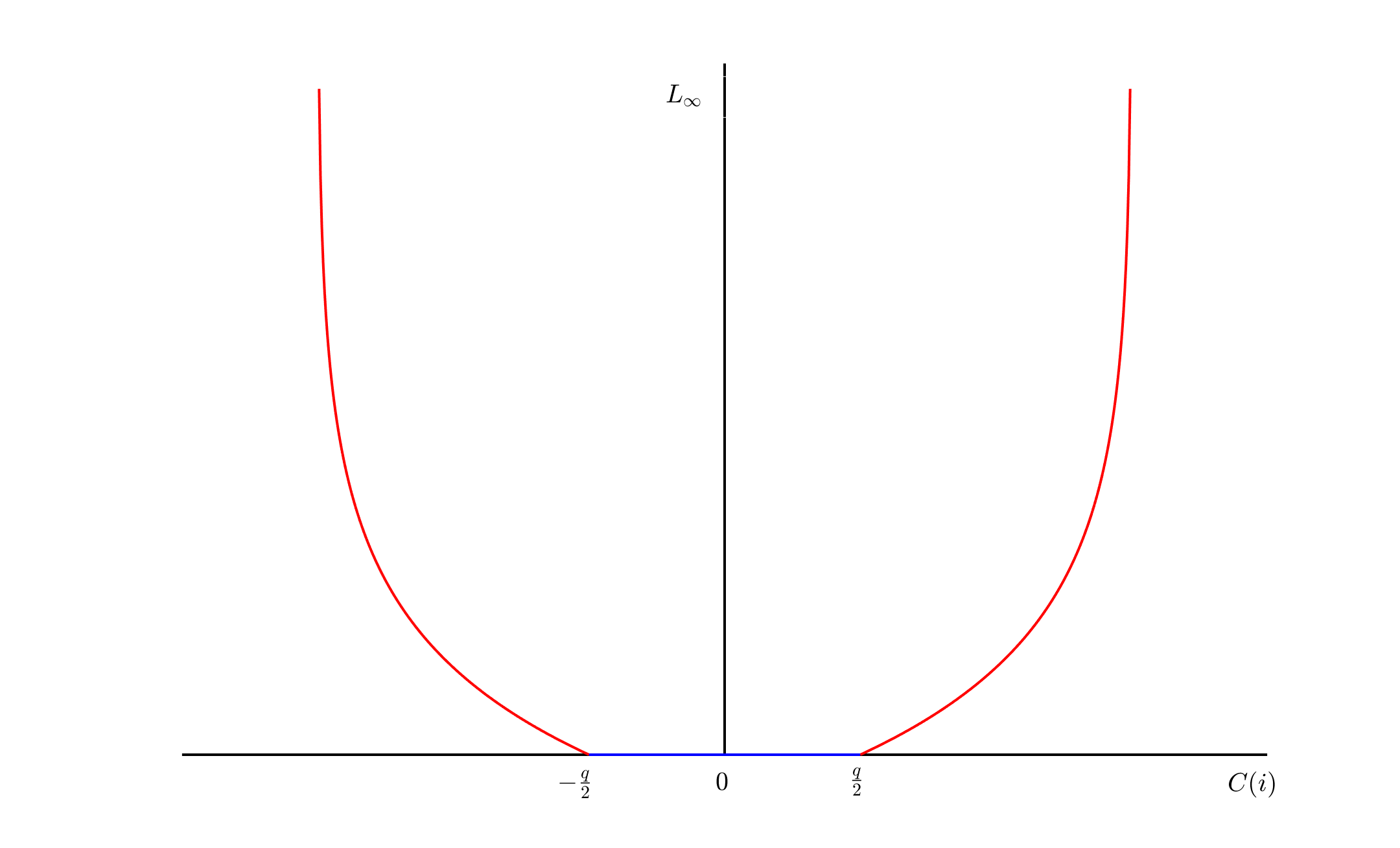
Fig. 2: The illustration of $L_{\infty}$ loss for one pixel

5 Locally Adaptive Illumination Compensation

As discussed in Section 3, the proposed DCNN technique learn the pattern of quantization artifacts from dynamic range stretched image patches generated using Eq. (7). Ideally, the proposed technique should work the best if the input image is also stretched by such a simple linear tone mapping. However, linear tone mapping, which adjusts the illumination of an image uniformly, is too restrictive in practice. For any image with a wide dynamic range, such as a photo containing both underexposed and normally exposed regions, linear tone mapping cannot enhance the dark regions sufficiently without saturating the details in the bright regions. Thus, it is necessary to adopt a locally adaptive approach for compensating the illumination of the input image.

There are plenty of tone mapping operators that can adjust image brightness locally [27, 28, 29, 30, 31], but none of these existing techniques fit all the requirements of the proposed approach. For an image with severely underexposed regions, the proposed dequantization neural network needs each of these regions to be stretched as uniformly as possible, just like a uniform increase of illumination as modelled in Eq. (1). Additionally, the tone mapped image should also exhibit good contrast, making local detail more visible to human viewers. Combining these two requirements together results a new formulation for low-light or uneven-light image tone mapping, namely locally adaptive illumination compensation (LAIC) as follows,

$$\begin{array}[]{rl}\mbox{minimize}&\displaystyle\sum_{i=1}\left[D\left(\tilde{J}(i)/J_{a}(i)\right)-\lambda_{2}\left|\tilde{J}(i)-\bar{J}(i)\right|\right]\\ \mbox{subject to}&0\leq\tilde{J}(i)\leq 1,\\ &\operatorname{sgn}\left(\tilde{J}(i)-\bar{J}(i)\right)=\operatorname{sgn}\left(J_{a}(i)-\bar{J}_{a}(i)\right),\end{array}$$ (19)

where the enhanced image $\tilde{J}$ is the variable, and the original low-light image $J_{a}$ is constant to the problem. Operator $\operatorname{sgn}(\cdot)$ is the sign function. Variable $\bar{J}(i)$ represents the average pixel intensity of image $\tilde{J}$ in the neighbourhood $\mathcal{D}_{i}$ of pixel $i$, i.e.,

$$\bar{J}(i)=\frac{1}{|\mathcal{D}_{i}|}\sum_{k\in\mathcal{D}_{i}}\tilde{J}(k).$$ (20)

Similarly, $\bar{J}_{a}(i)$ is the local average of $J_{a}(i)$. For a pixel of image $I$ with coordinate $(u,v)$, derivative operator $D\left(I(u,v)\right)$ is defined as follows,

$$D\left(I(u,v)\right) =|I(u+1,v)-I(u,v)|$$

$$\quad+|I(u,v+1)-I(u,v)|.$$ (21)

The problem in Eq. (19) optimizes two objectives: the total variation of illumination gain and the local contrast of the enhanced image. Minimizing the total variation of illumination gain $\tilde{J}(i)/J_{a}(i)$ is to find a solution with piece-wise constant illumination gain. Maximizing the local contrast is to boost the detail of the output image. The importance of the two often conflicting objectives are balanced with a user given Lagrange multiplier $\lambda_{2}$.

The first constraint of the optimization problem in Eq. (19) is to bound the dynamic range of the enhanced image $\tilde{J}$ to $[0,1]$. The second constraint is to preserve the rank of each pixel to its local average. For instance, if a pixel of the input image is brighter than the average pixel value in the neighbourhood of the pixel, then the same must also be true in the enhanced output image by this constraint. By preserving the rank in local regions, a method can be perceptually free of many tone mapping artifacts such as Halo and double edge.

This optimization problem is non-convex and difficult to solve directly, however, since the enhanced image $\tilde{J}$ preserves the rank between each pixel and its local average, $\tilde{J}(i)-\bar{J}(i)$ always shares the same sign with $J_{a}(i)-\bar{J}_{a}(i)$. Thus,

$$\left|\tilde{J}(i)\!-\!\bar{J}(i)\right| =\left(\tilde{J}(i)\!-\!\bar{J}(i)\right)\cdot\operatorname{sgn}\left(\tilde{J}(i)\!-\!\bar{J}(i)\right)$$

$$=\left(\tilde{J}(i)\!-\!\bar{J}(i)\right)\cdot\operatorname{sgn}\left(J_{a}(i)\!-\!\bar{J}_{a})\right)$$ (22)

Since $J_{a}(i)$ and $\bar{J}_{a}(i)$ are constant to the optimization problem in Eq. (19), the local contrast term of the objective function is linear. On the other hand, the total variation of illumination gain term can also be reformulate as a linear function. Thus, the objective function of the problem is linear. The local rank preserving constraints in Eq. 19 can also be written as equivalent linear inequalities as follows,

$$\left\{\begin{array}[]{rr}\tilde{J}(i)-\bar{J}(i)\leq 0&\text{if $J_{a}(i)\leq\bar{J}_{a}(i)$},\\ \tilde{J}(i)-\bar{J}(i)\geq 0&\text{if $J_{a}(i)\geq\bar{J}_{a}(i)$}.\\ \end{array}\right.$$ (23)

Therefore, this reformulated LAIC problem is a tractable linear program.

6 Experimental Results

In this section, We compare our method with four of the state-of-the-art low-light image enhancement methods: CLAHE [6], OCTM [10], LIME [15] and SRIE [16]. The operation of CLAHE is executed on the V channel of images by first converting it from RGB colorspace to the HSV colorspace and then converting the proposed HSV back to the RGB colorspace. LLNeT [20] is not examined here, as the authors did not make the implementation available for evaluation. We evaluate the tested methods on variety of data, including synthetic images, high dynamic range images and real photographs. Except for the first experiment on the synthetic global low-light images, we firstly enhance the images by LAIC, then restore the quantization residual using our trained network.

6.1 Experiments on Synthetic Images

(a) Input

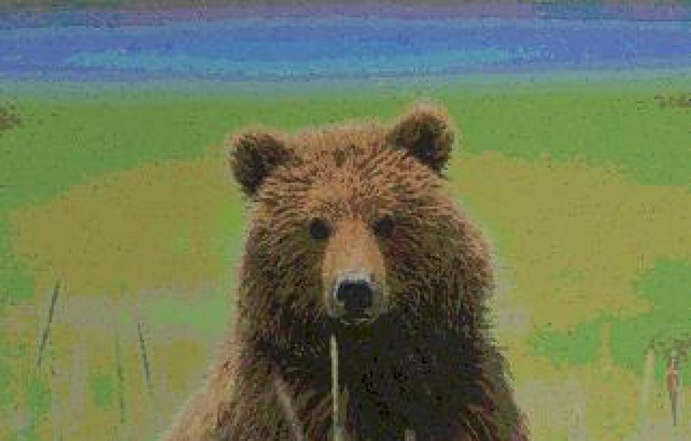
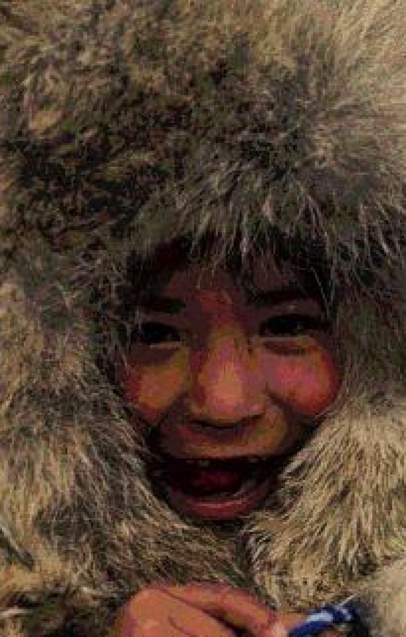
(b) CLAHE

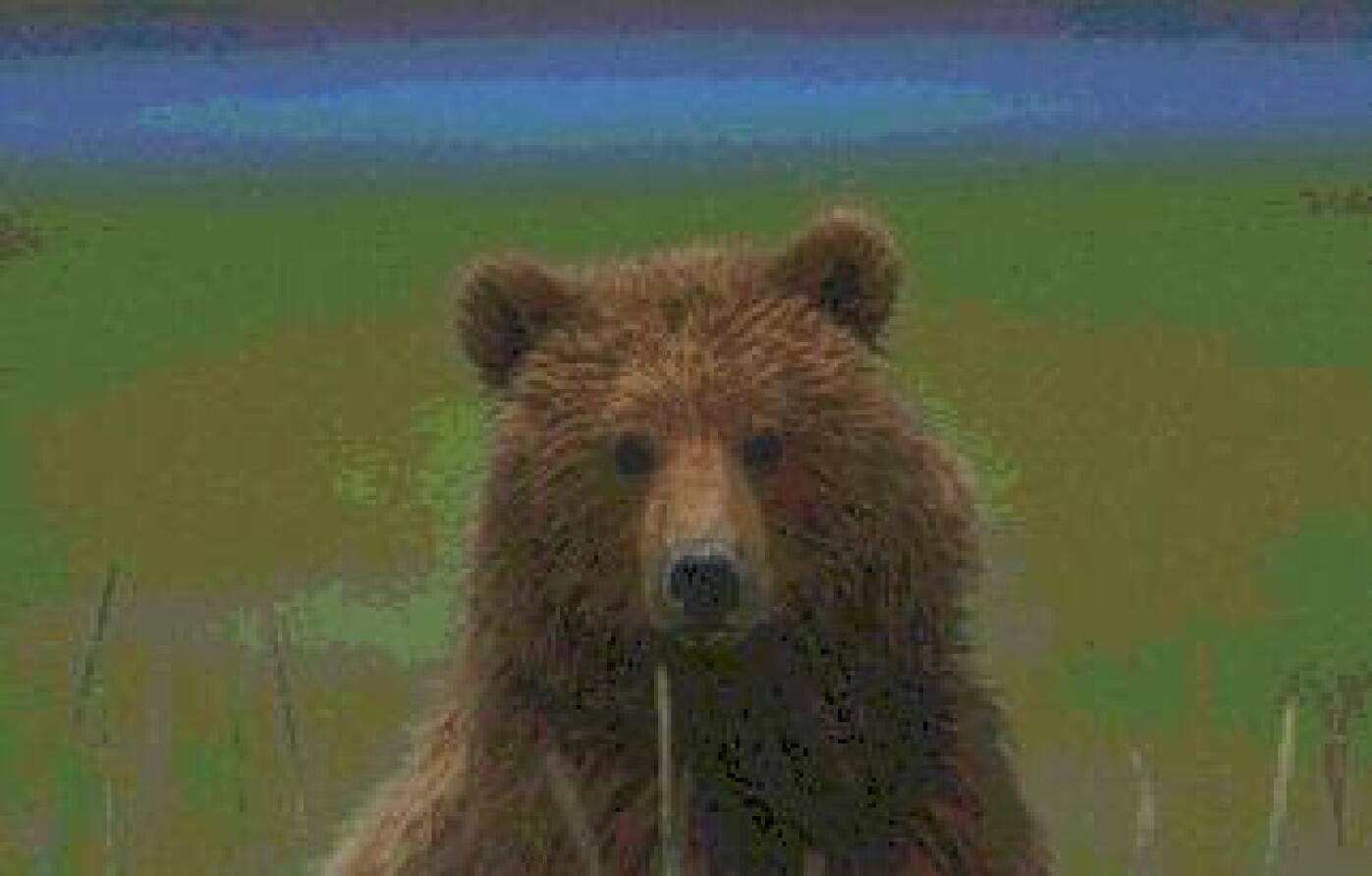
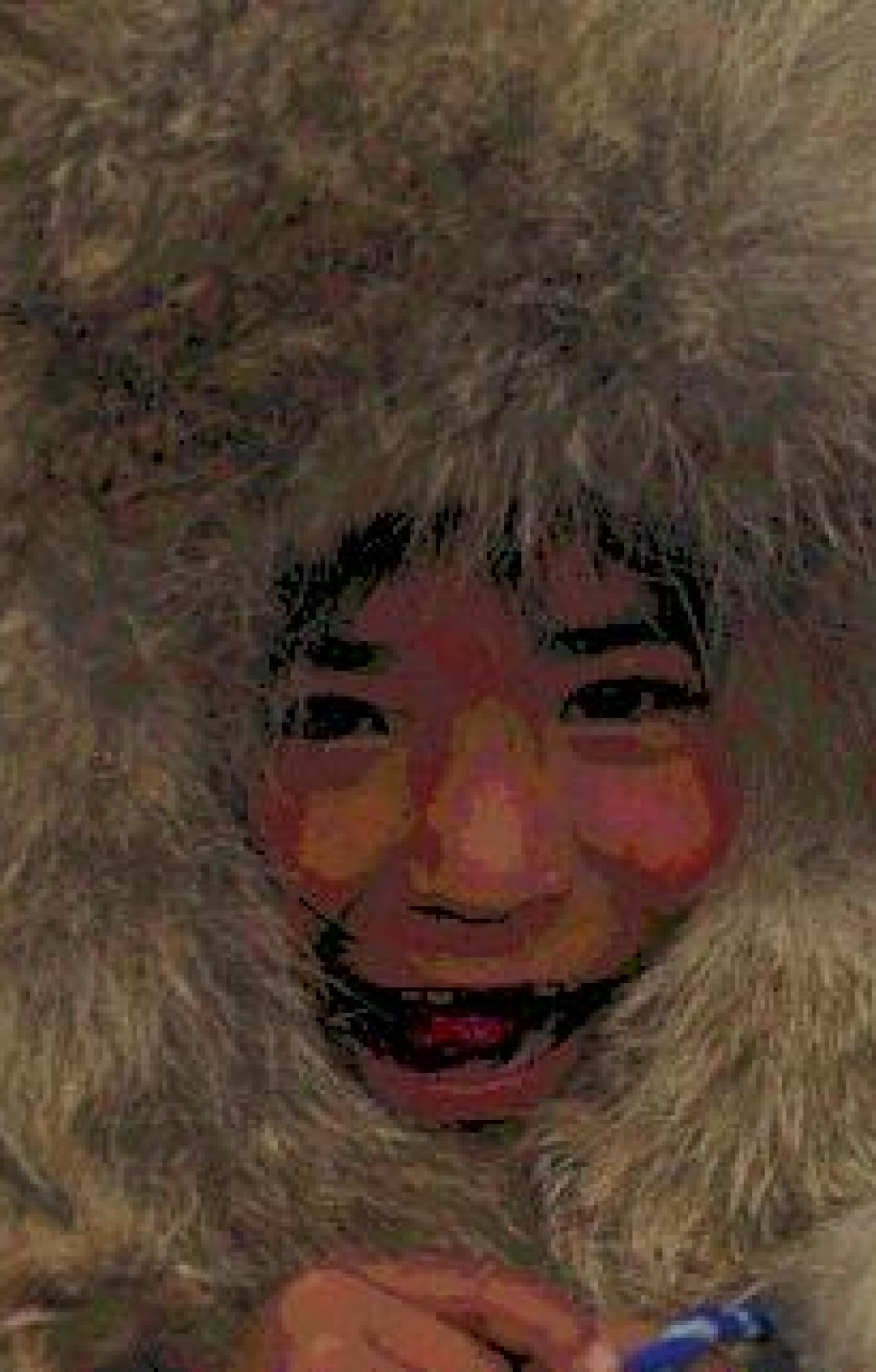
(c) OCTM

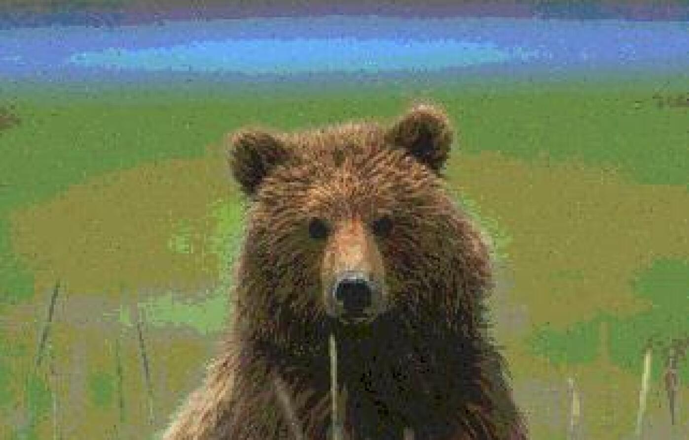
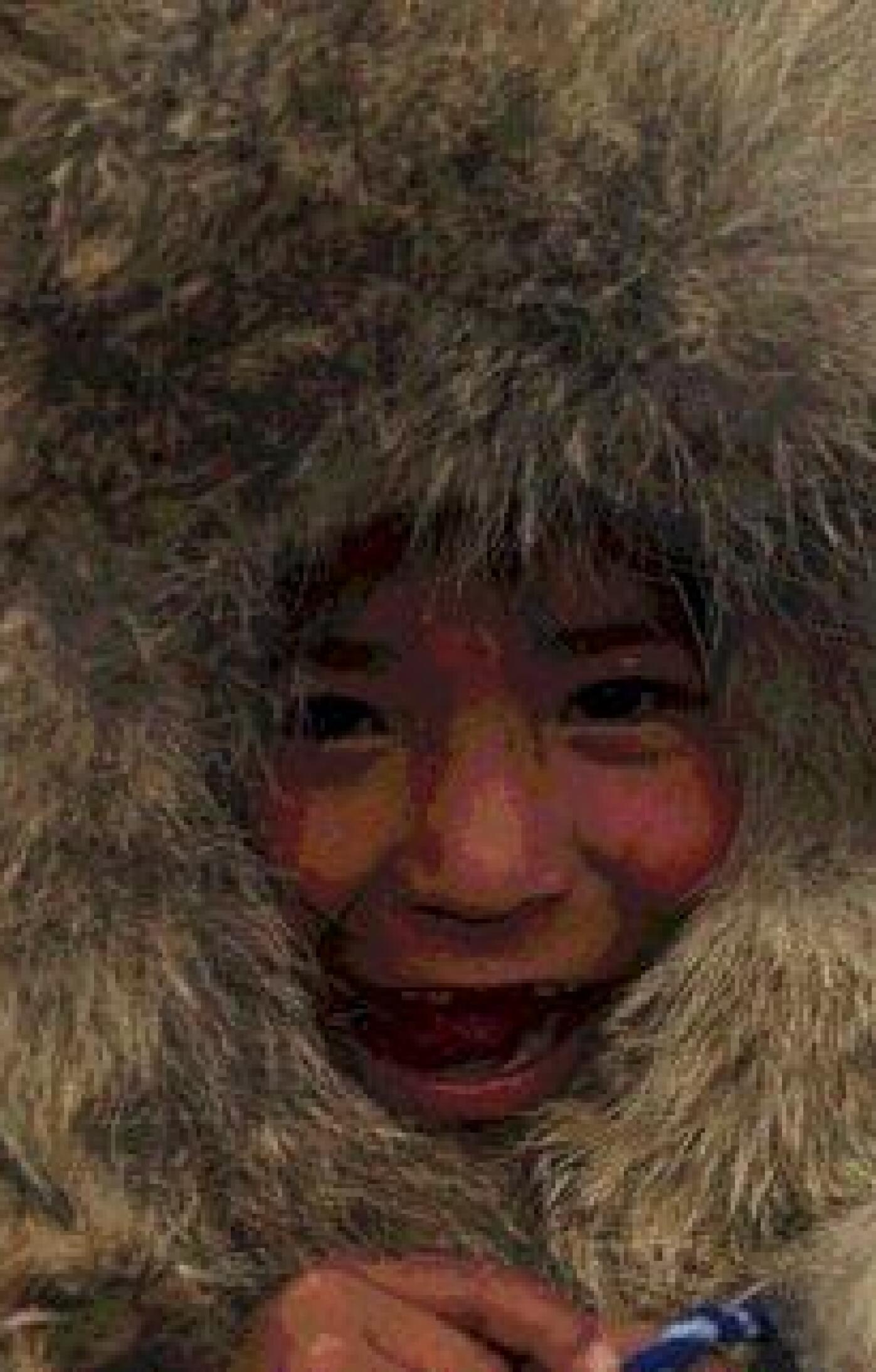
(d) LIME

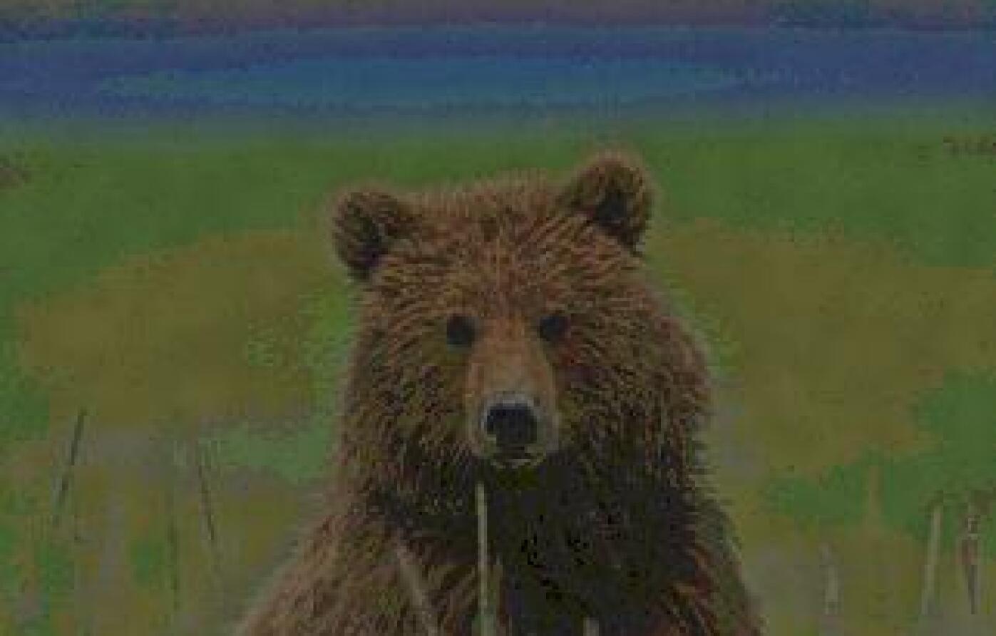
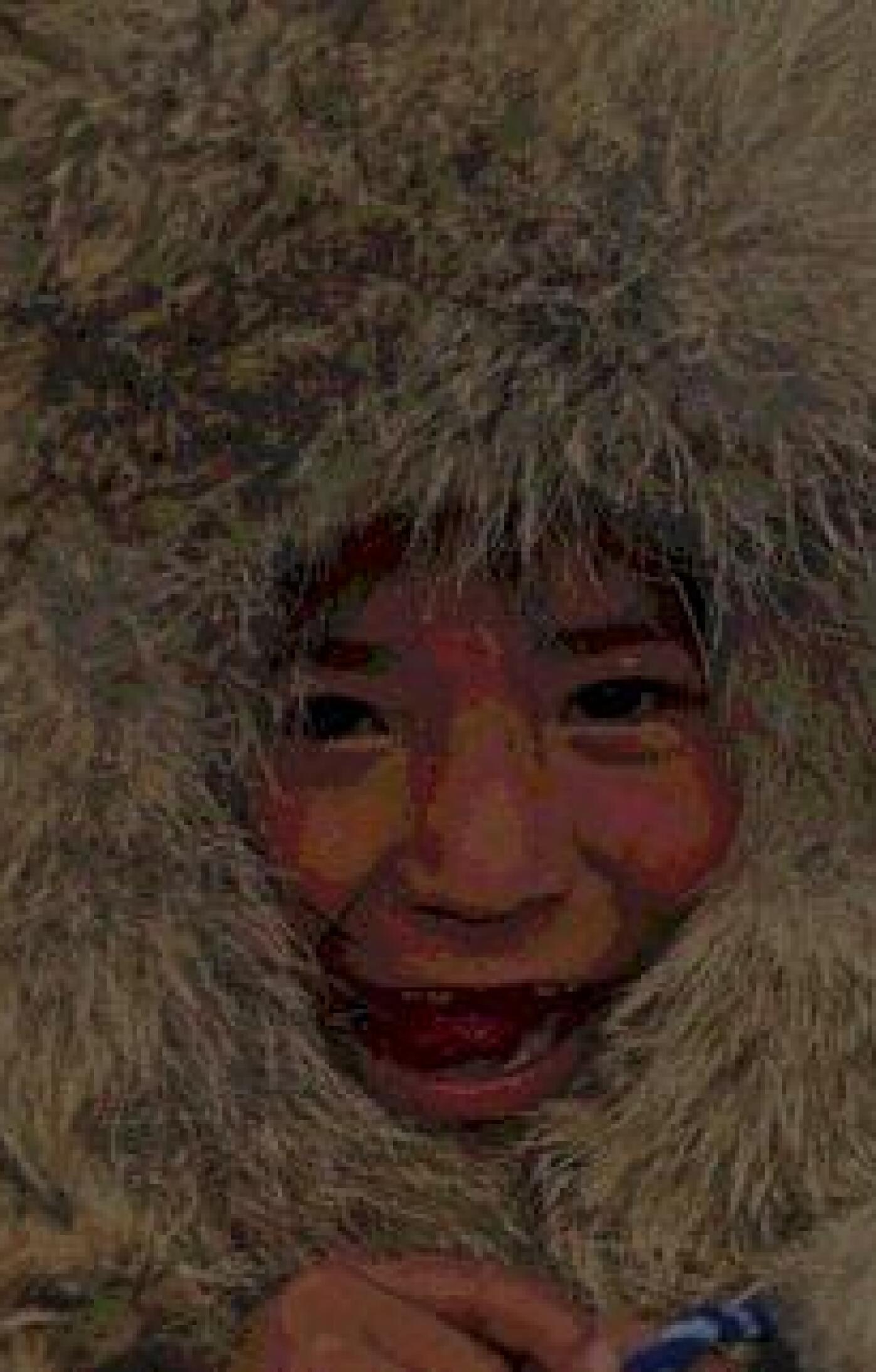
(e) SRIE

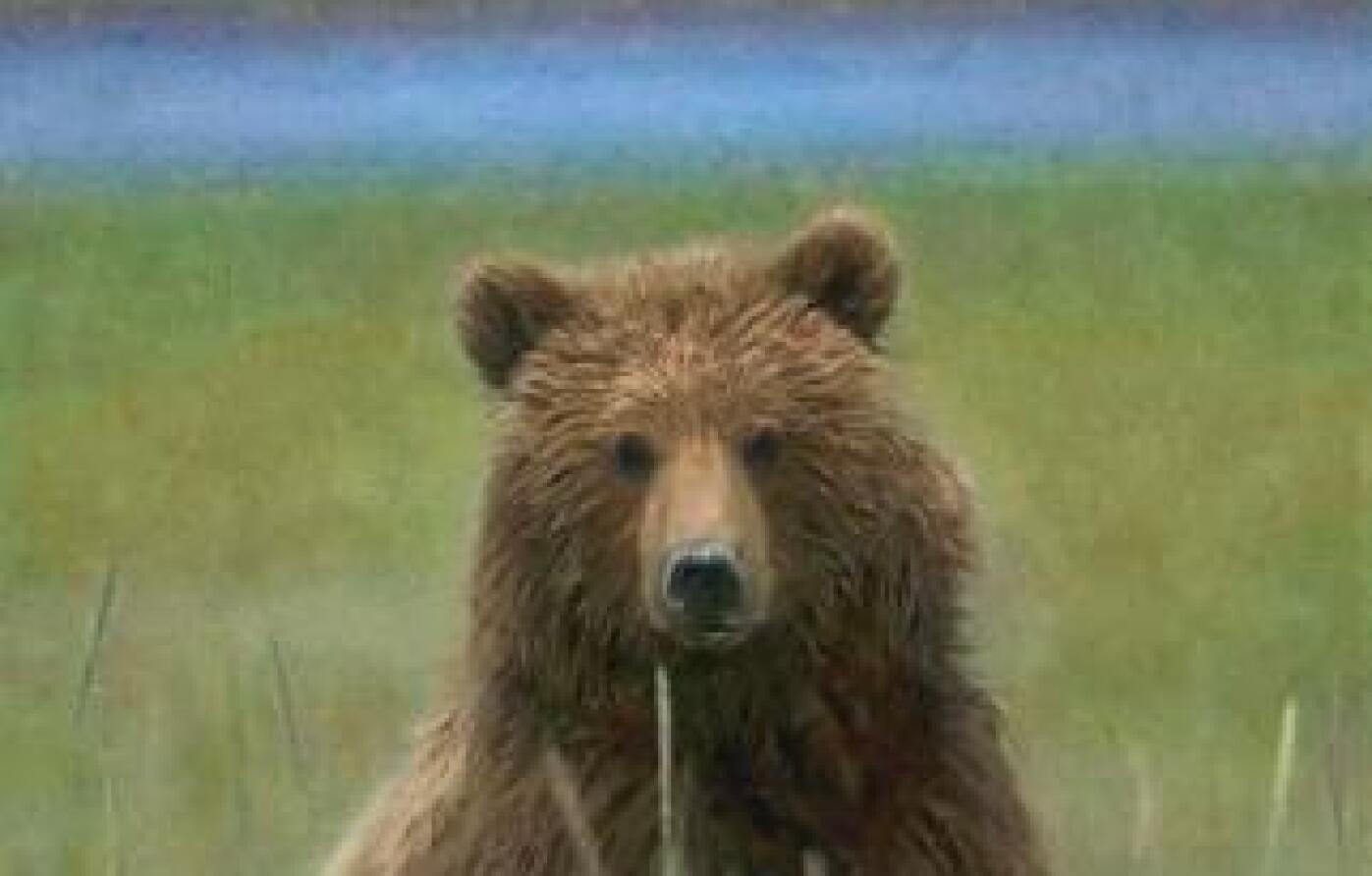
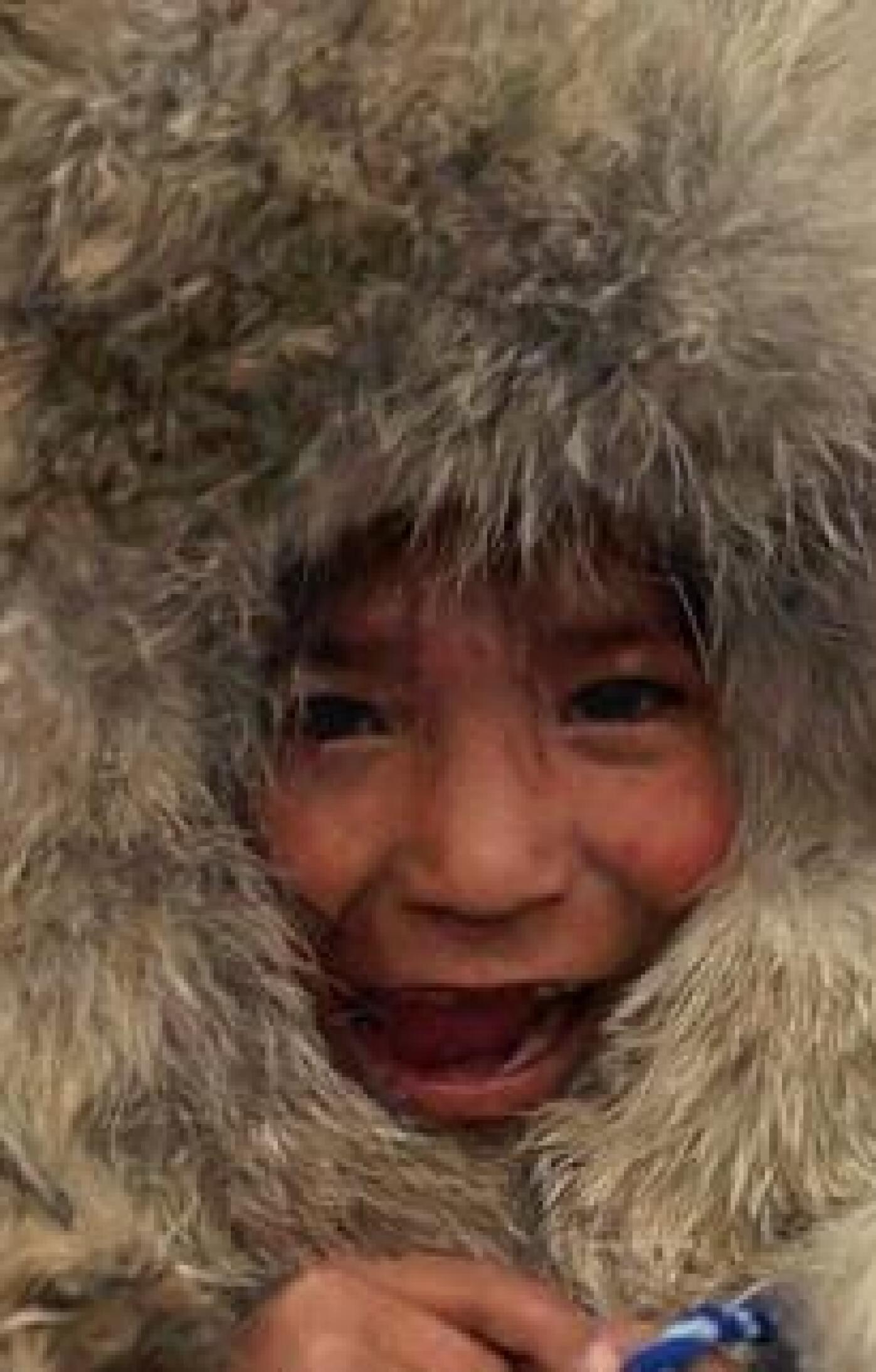
(f) Proposed

Fig. 3: Results of tested techniques for synthetic low-light images. In this experiment, the low-light images are linearly tone mapped before applying the proposed dequantization technique.

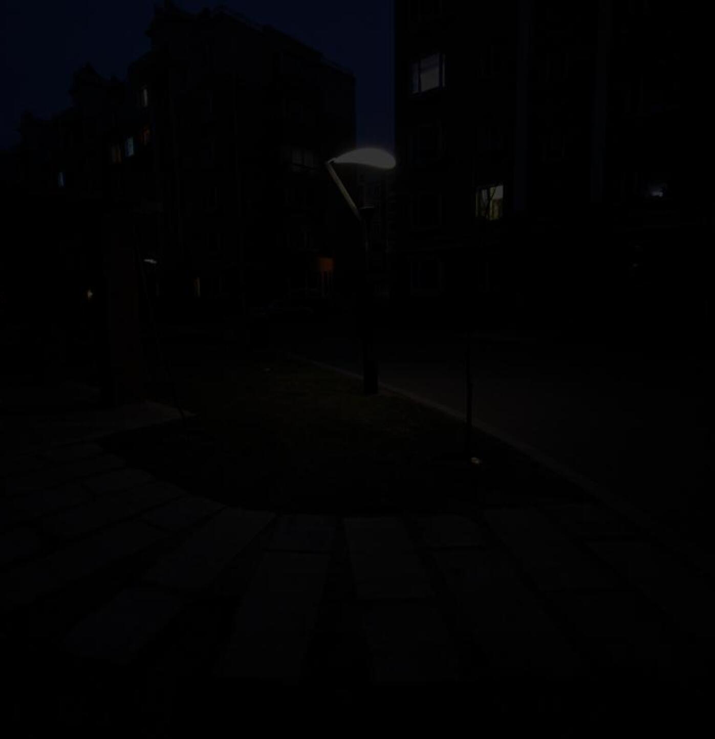
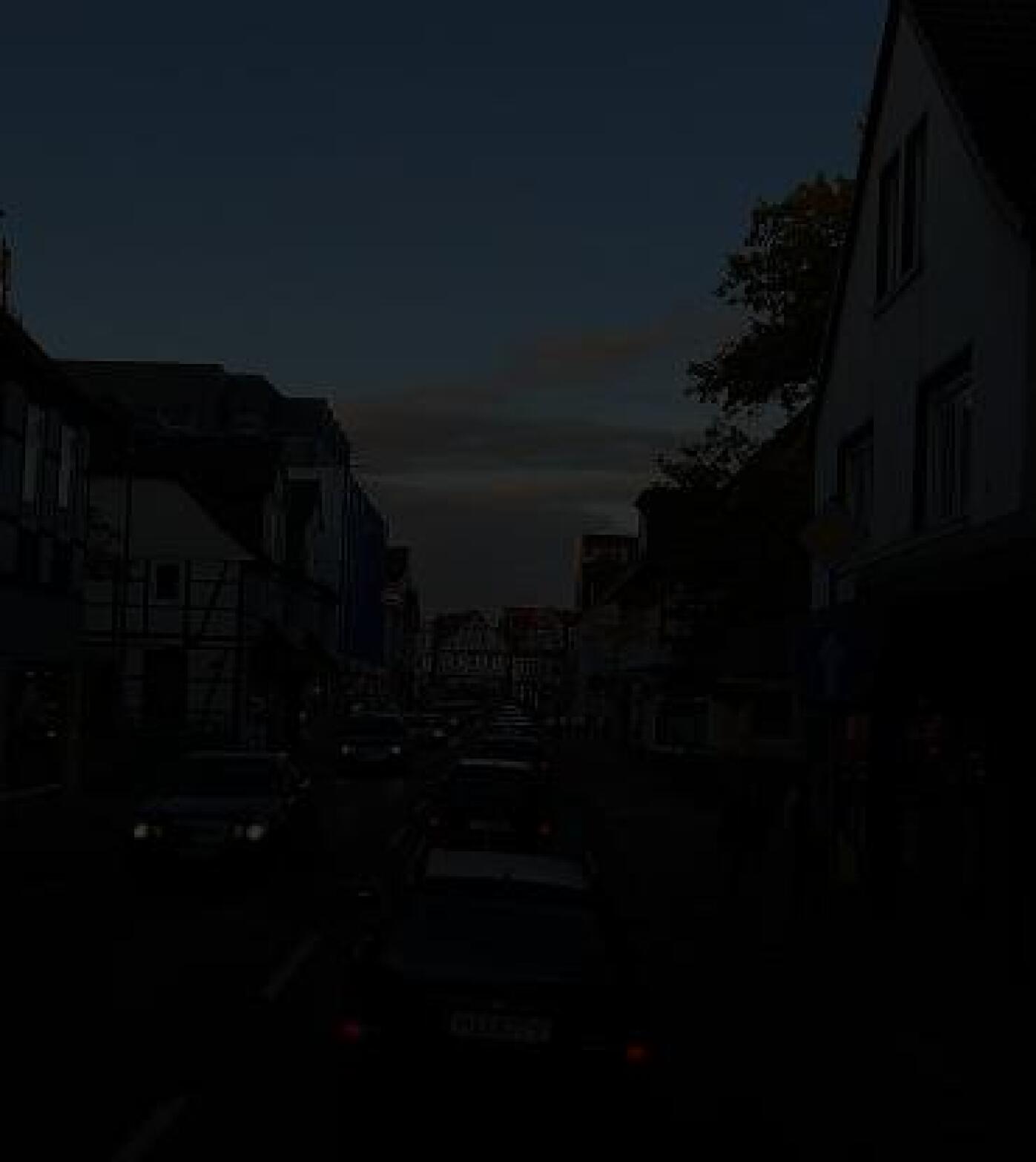
(a) Input

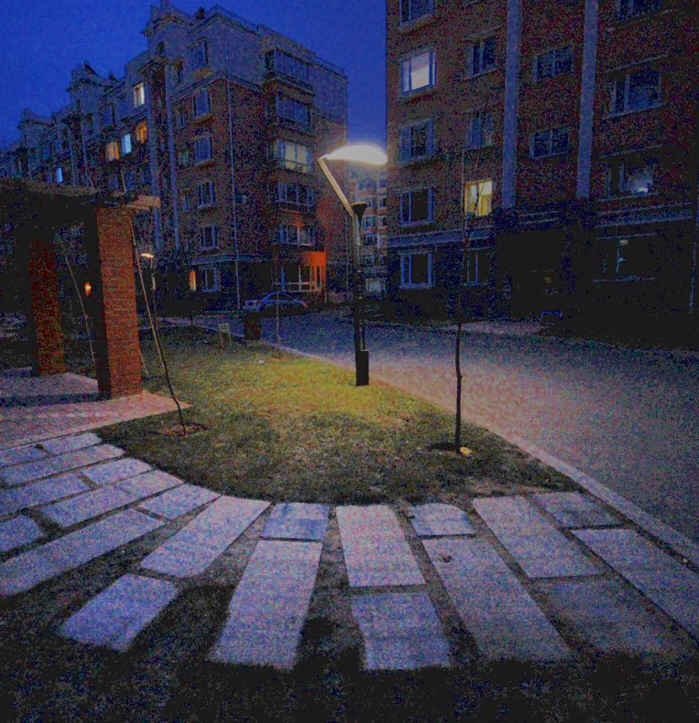
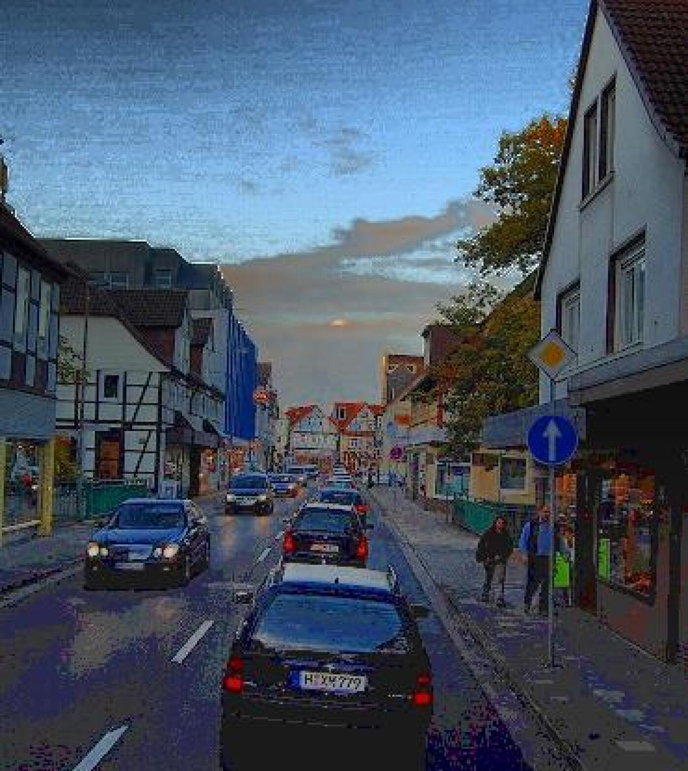
(b) CLAHE

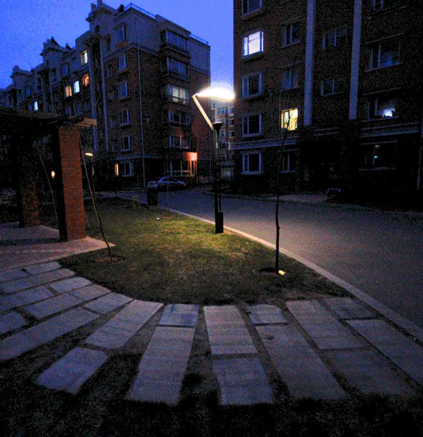
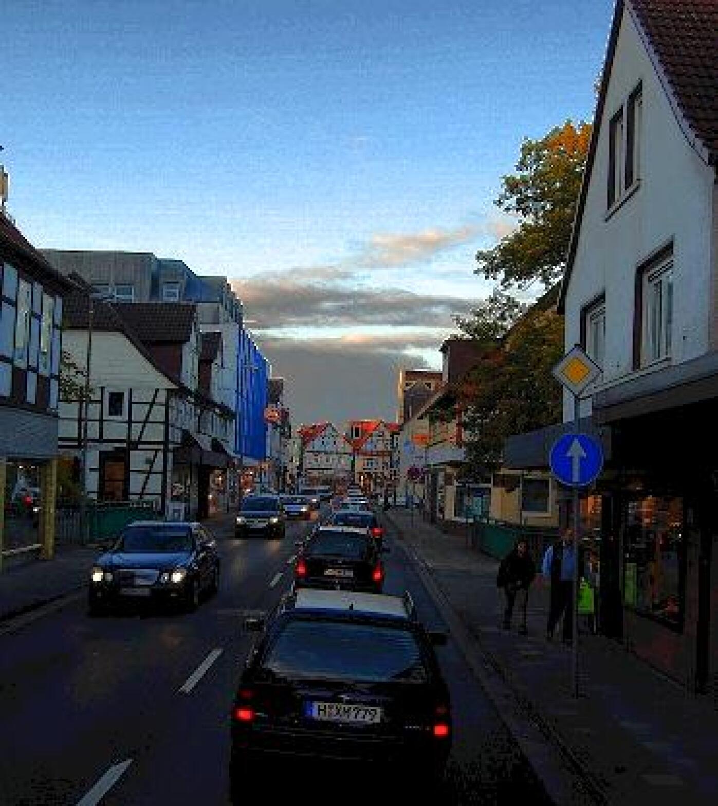
(c) OCTM

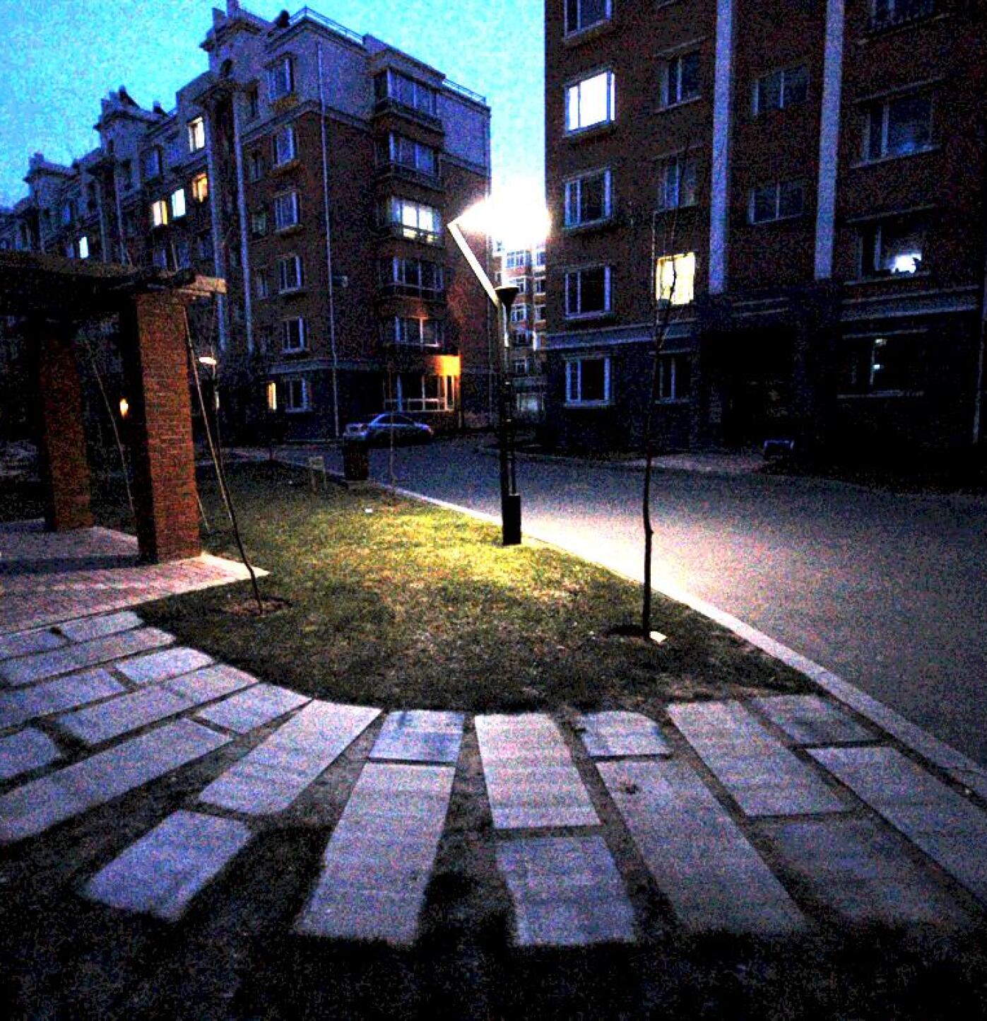
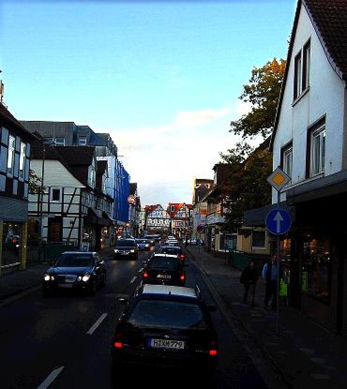
(d) LIME

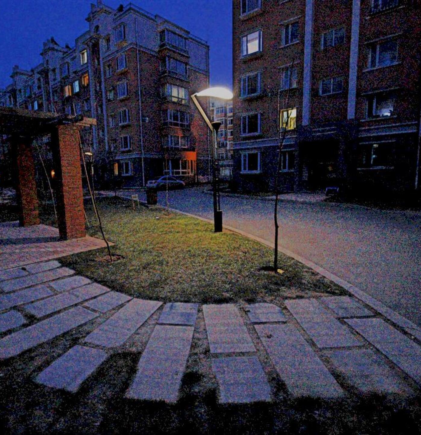
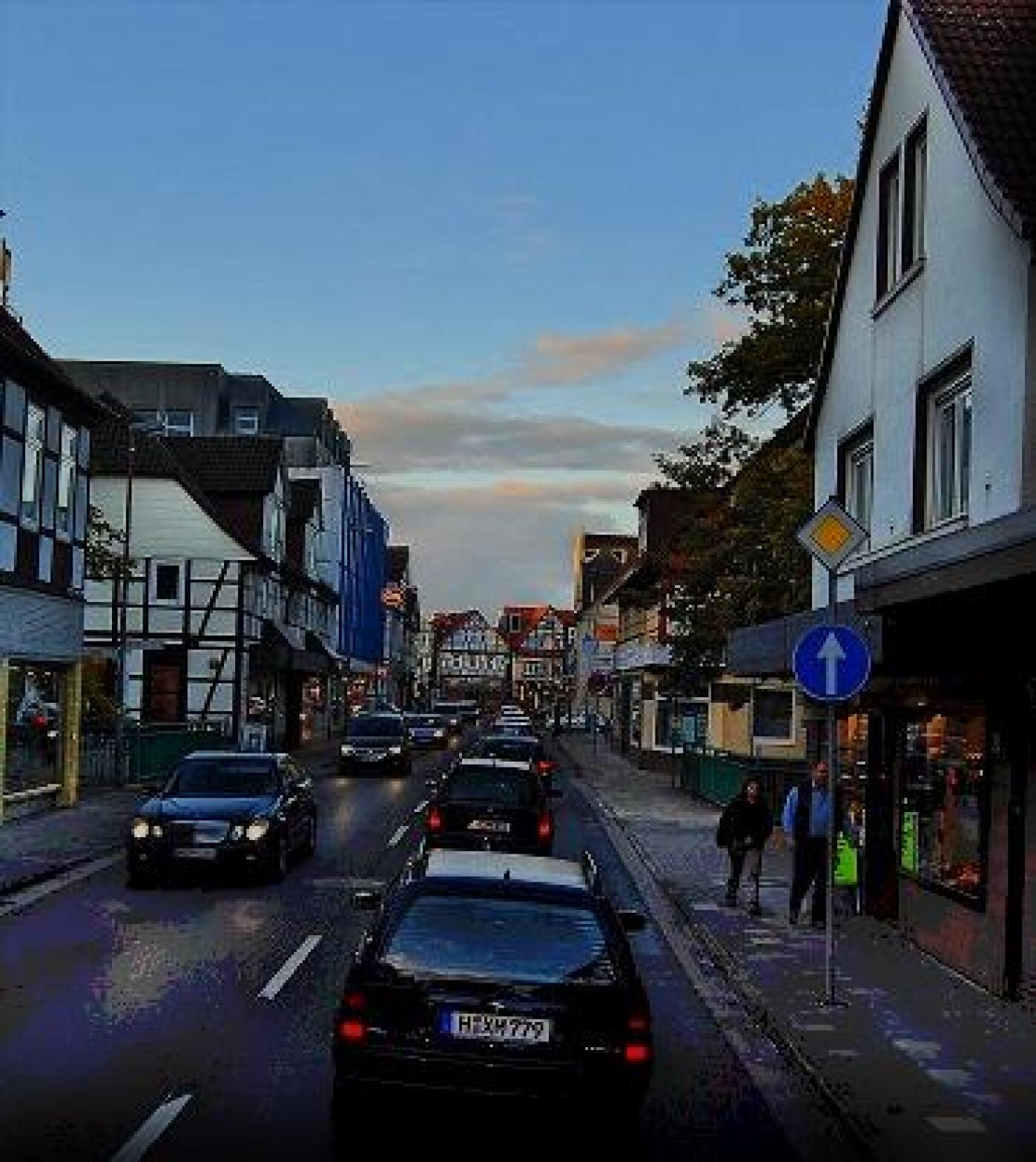
(e) SRIE

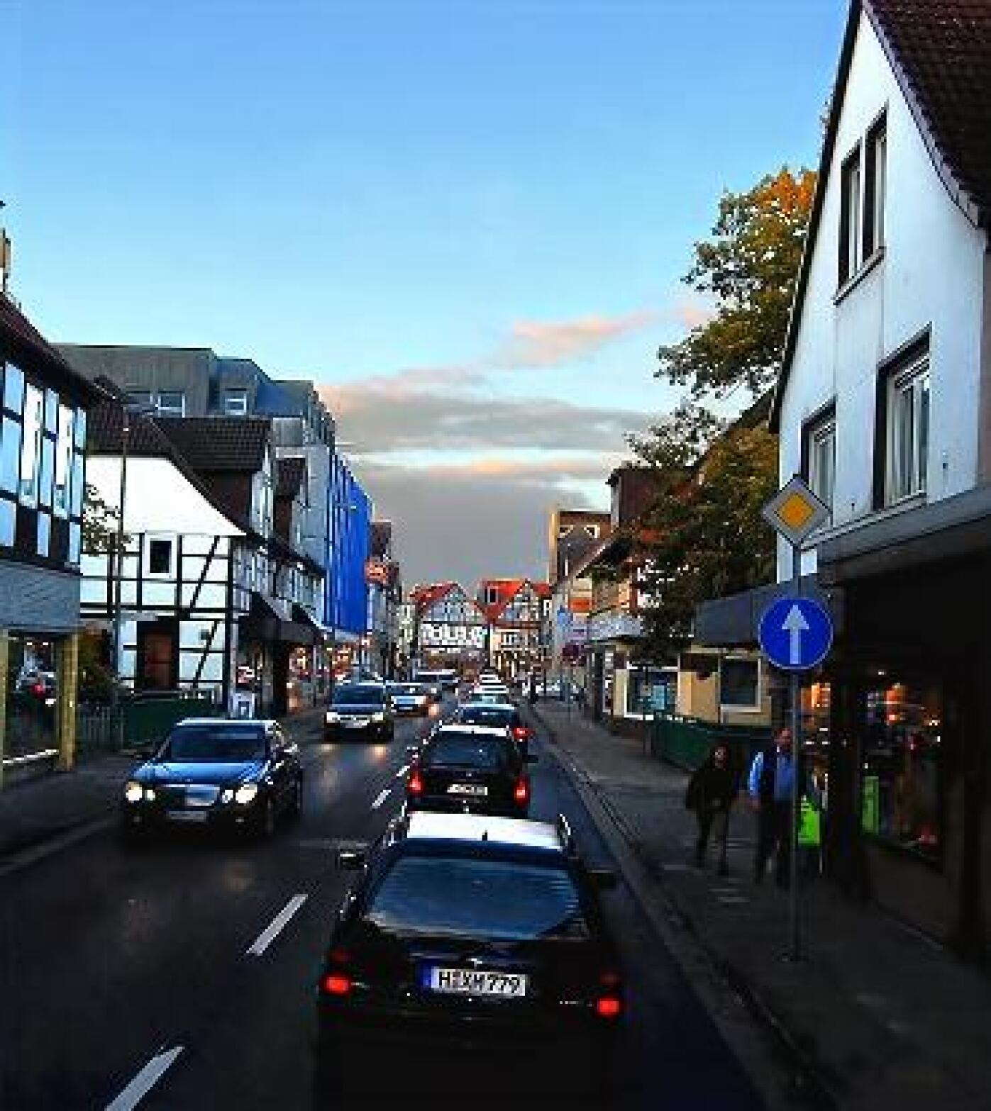
(f) Proposed

Fig. 4: Results of the tested techniques for synthetic low-light images. In this experiment, the low-light images are tone mapped by LAIC before applying the proposed dequantization technique.

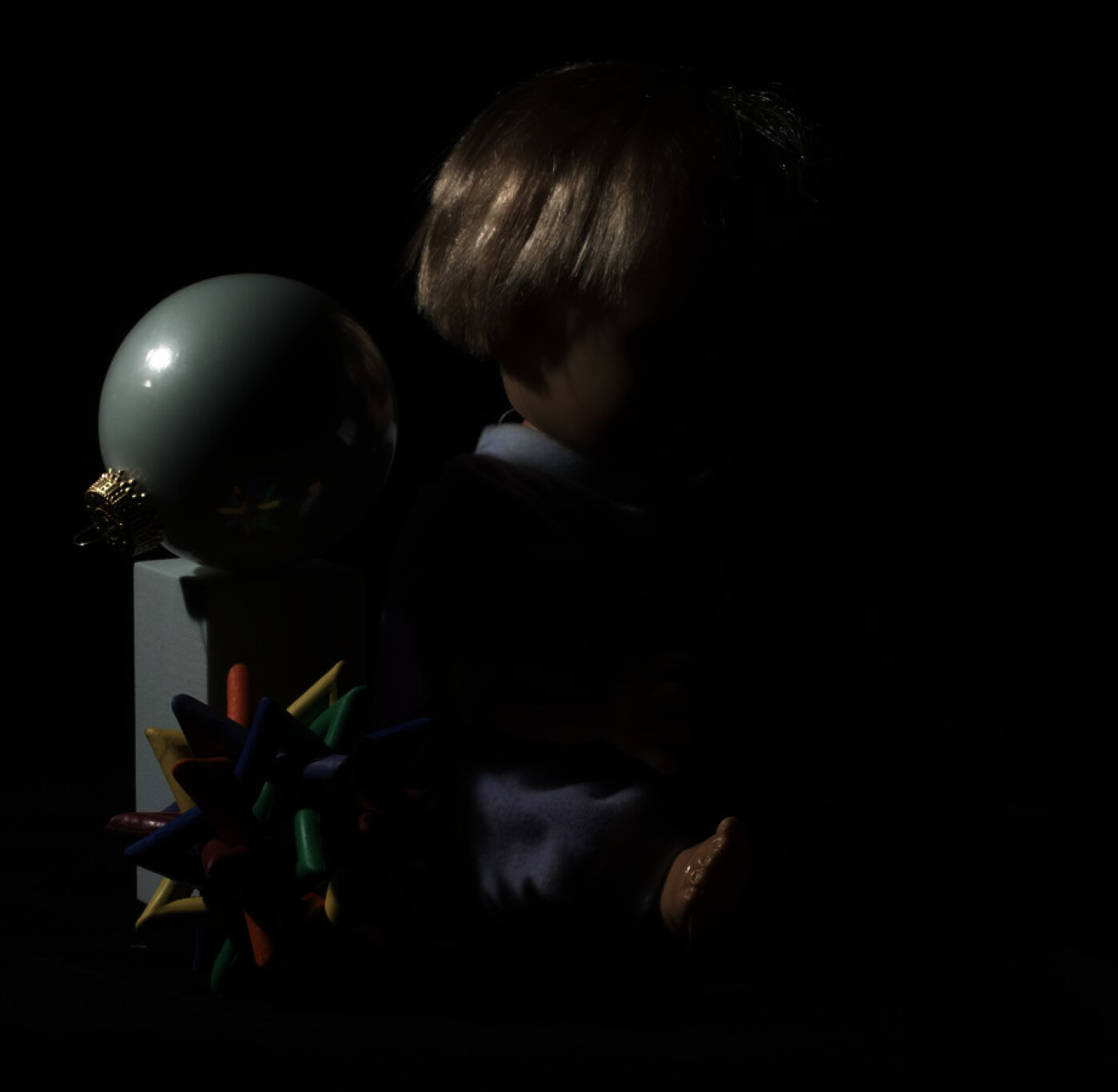
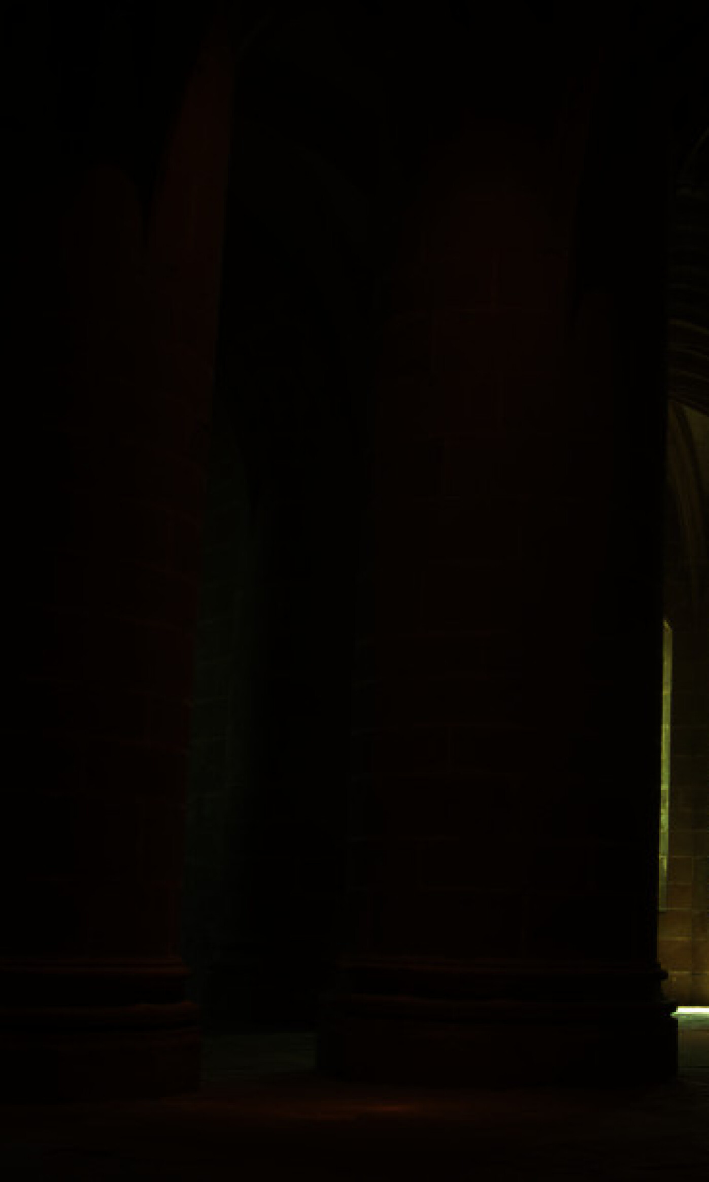
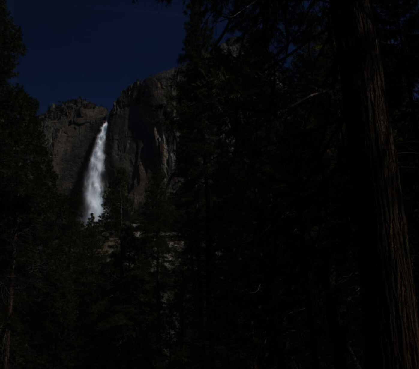
(a) Input

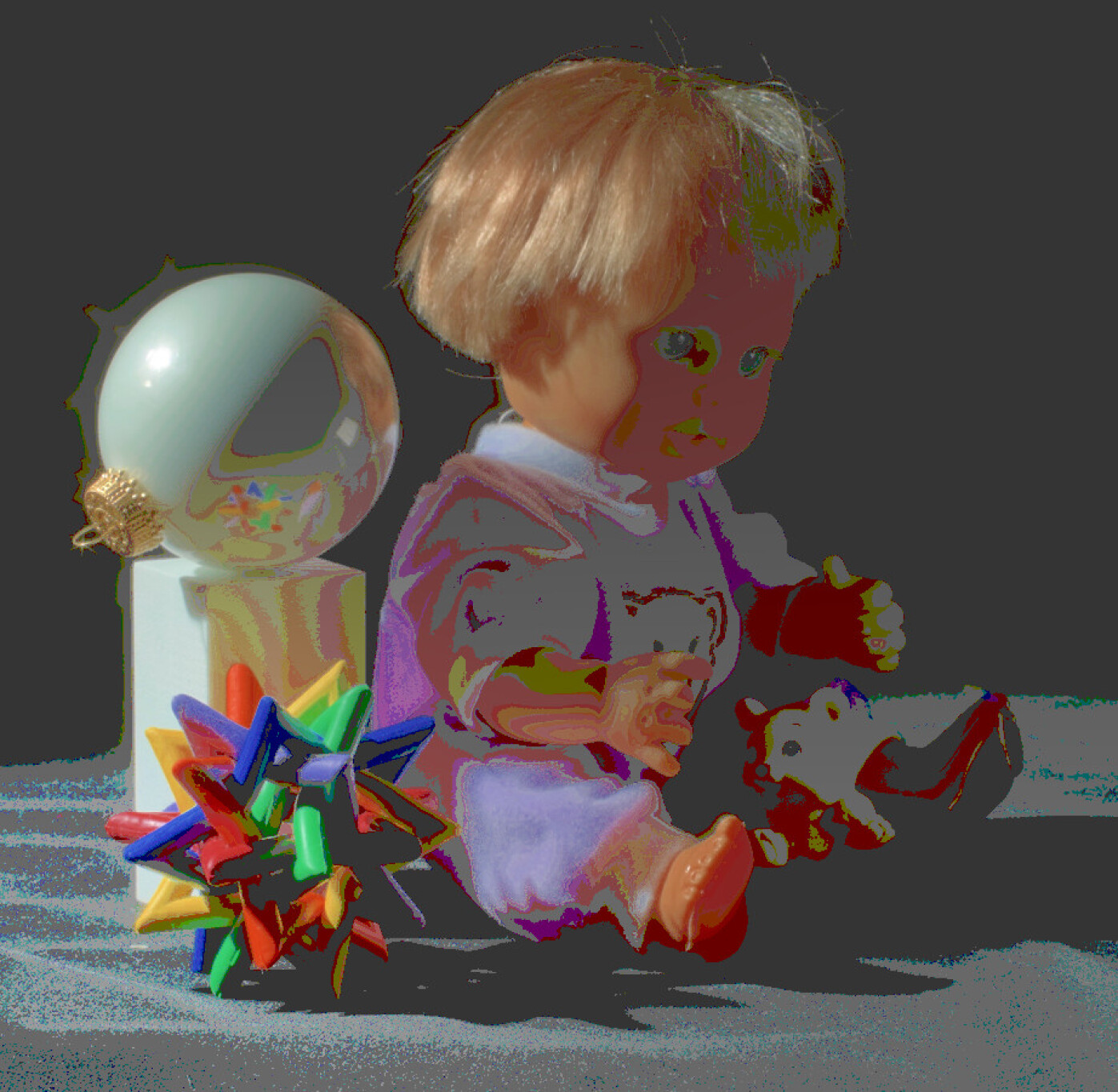
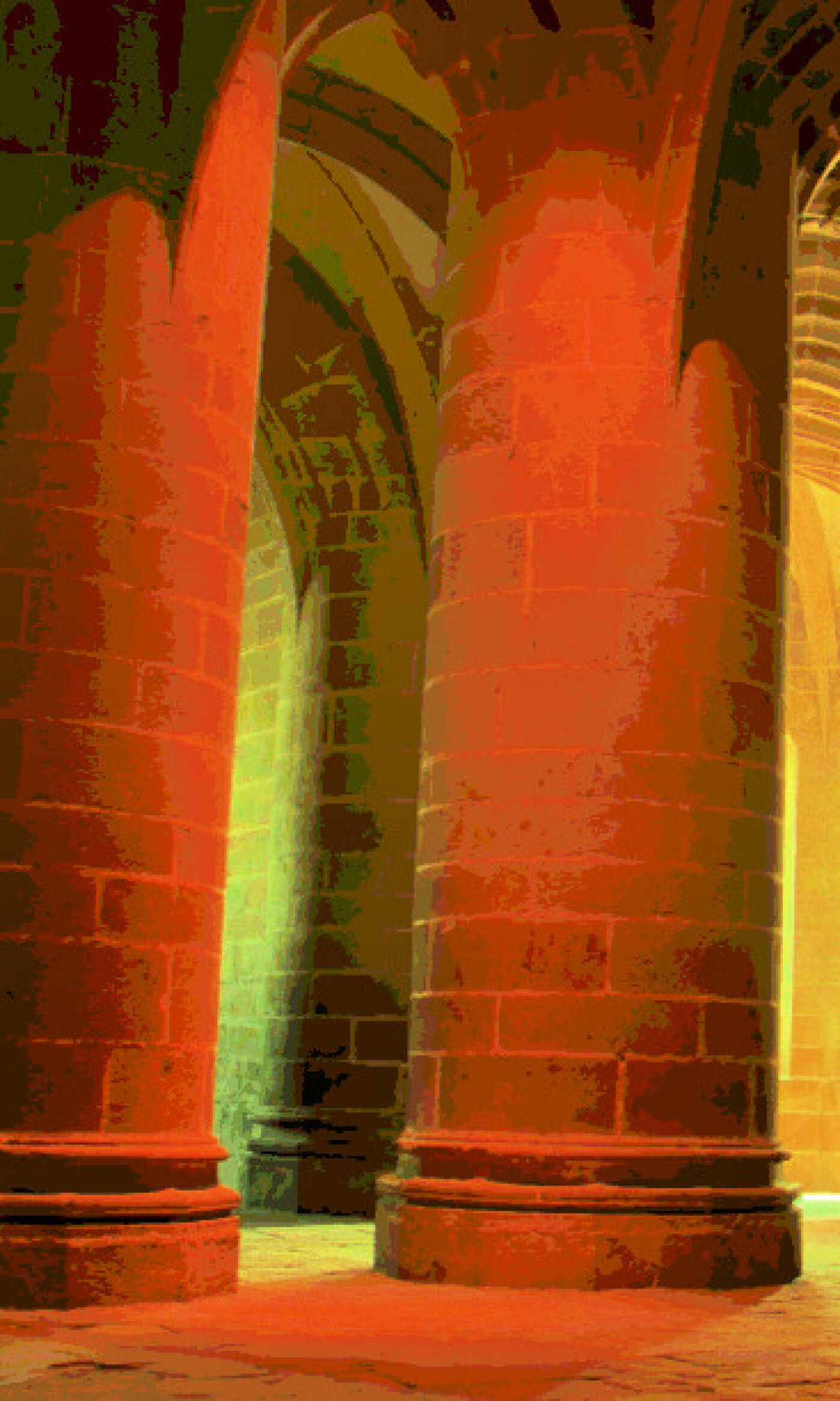
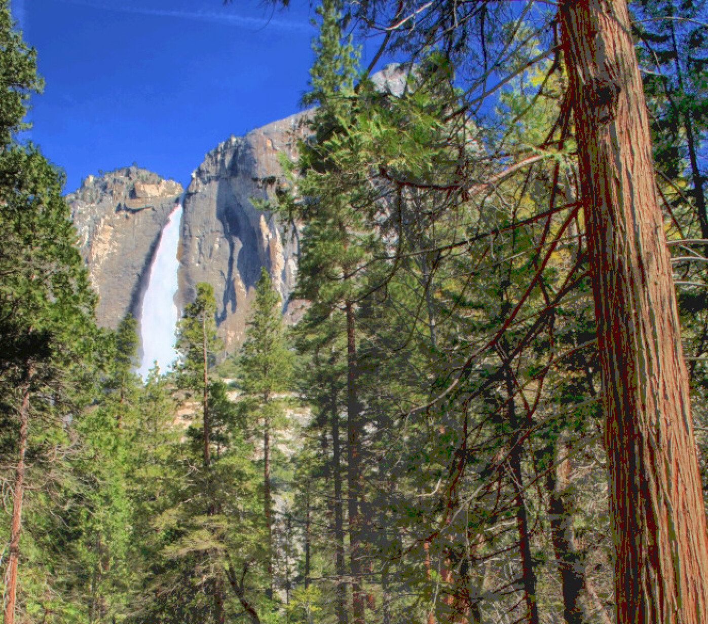
(b) CLAHE

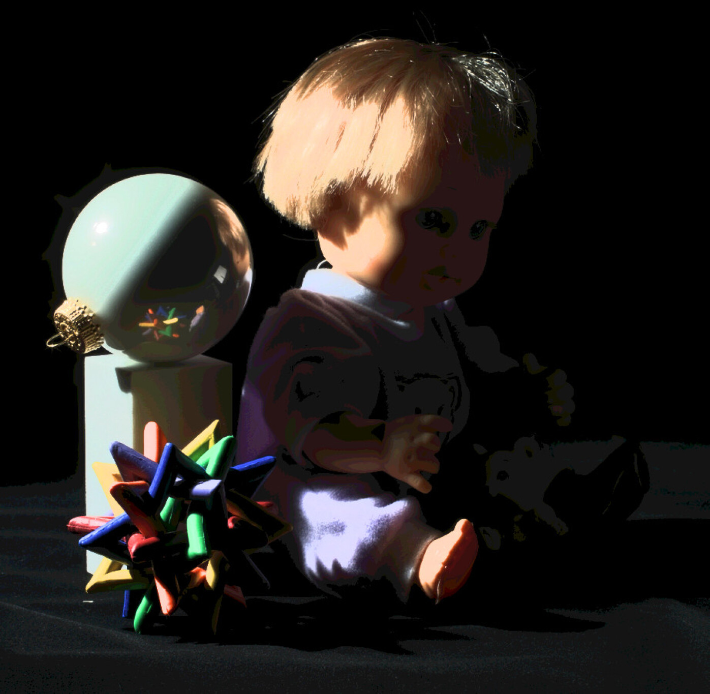
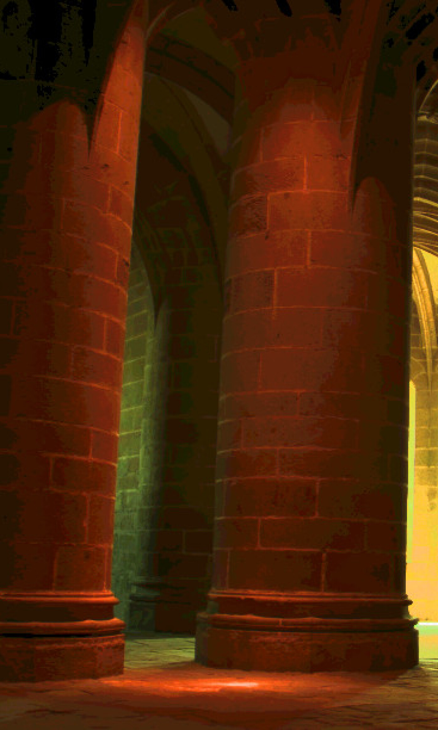
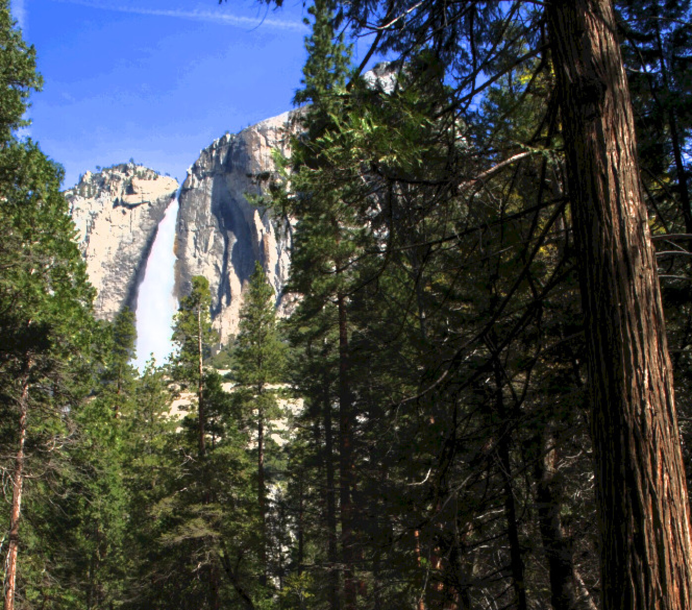
(c) OCTM

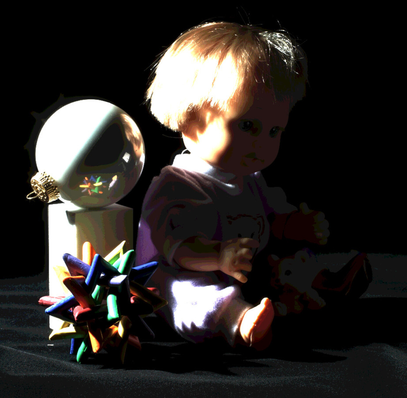
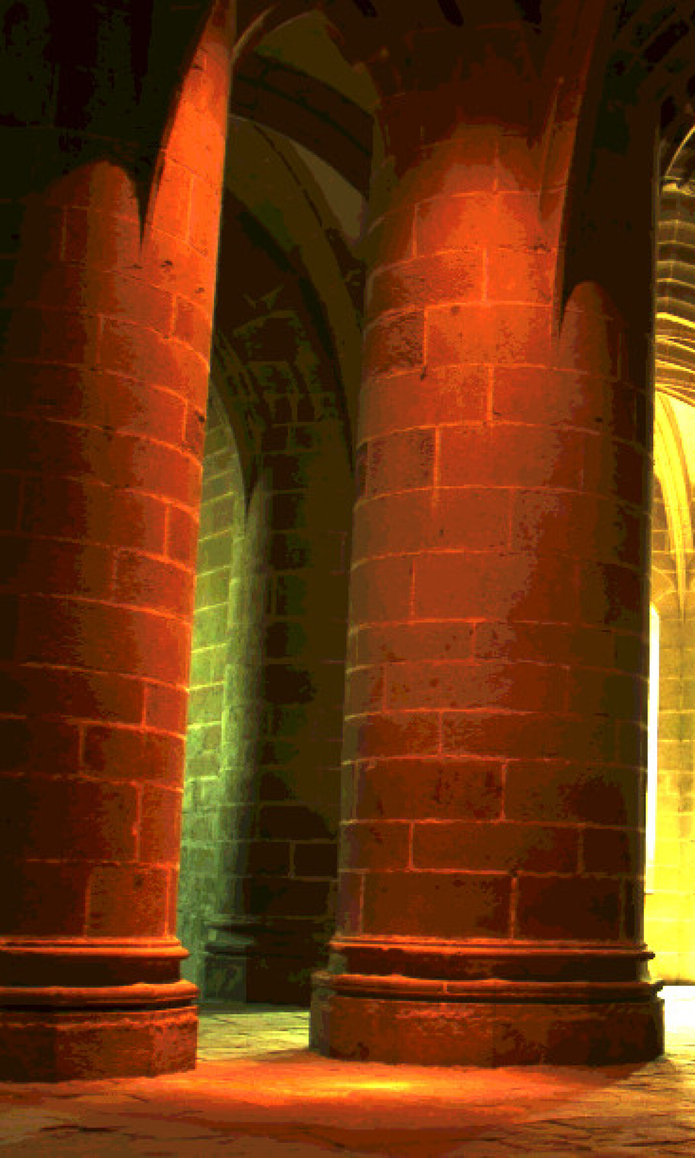
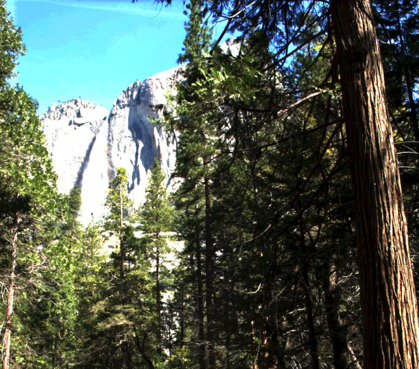
(d) LIME

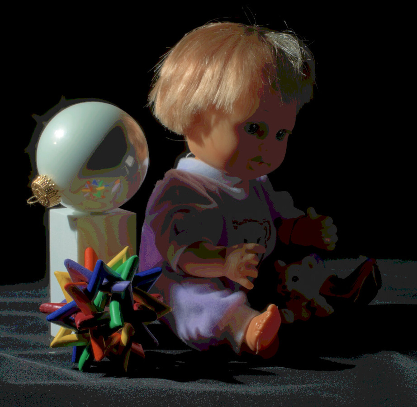
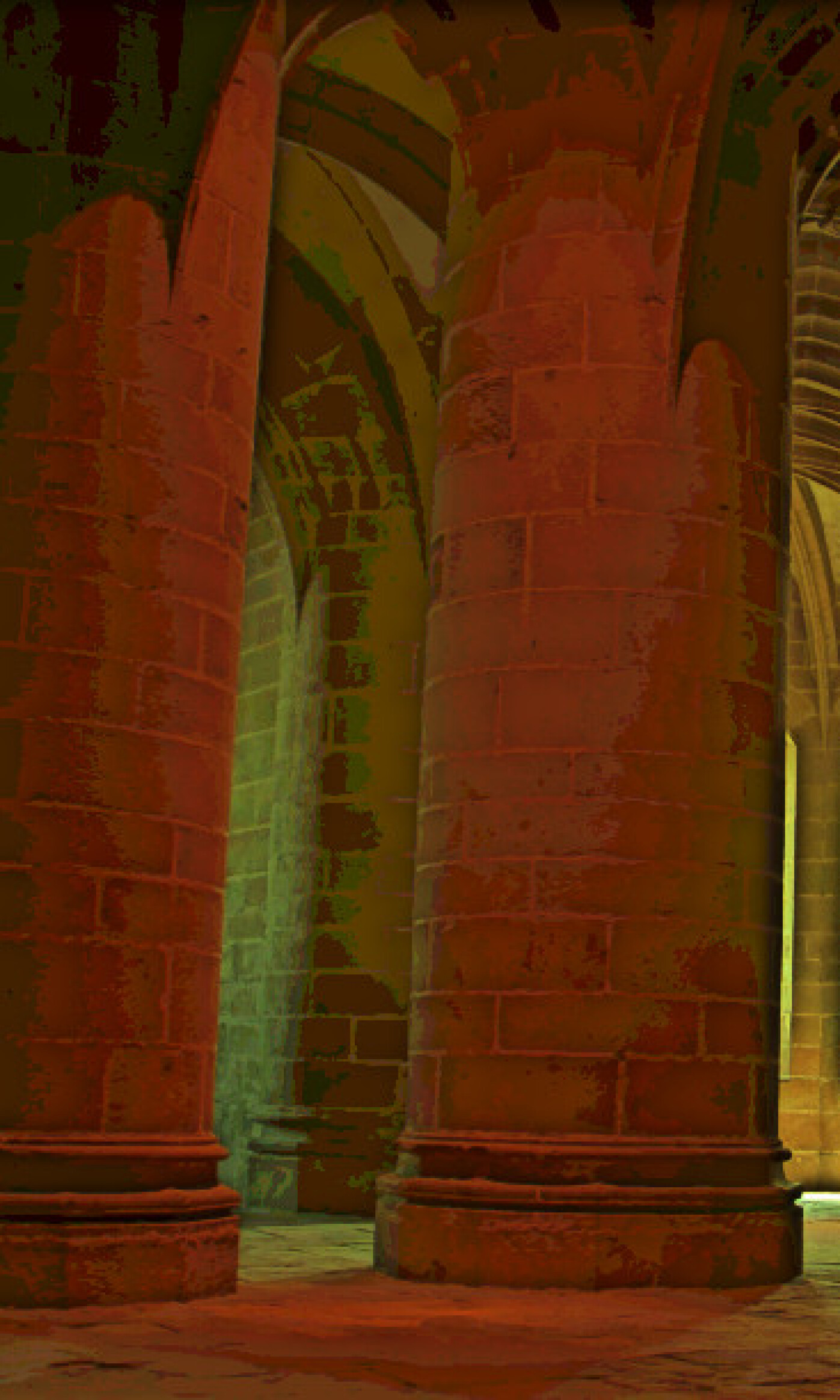
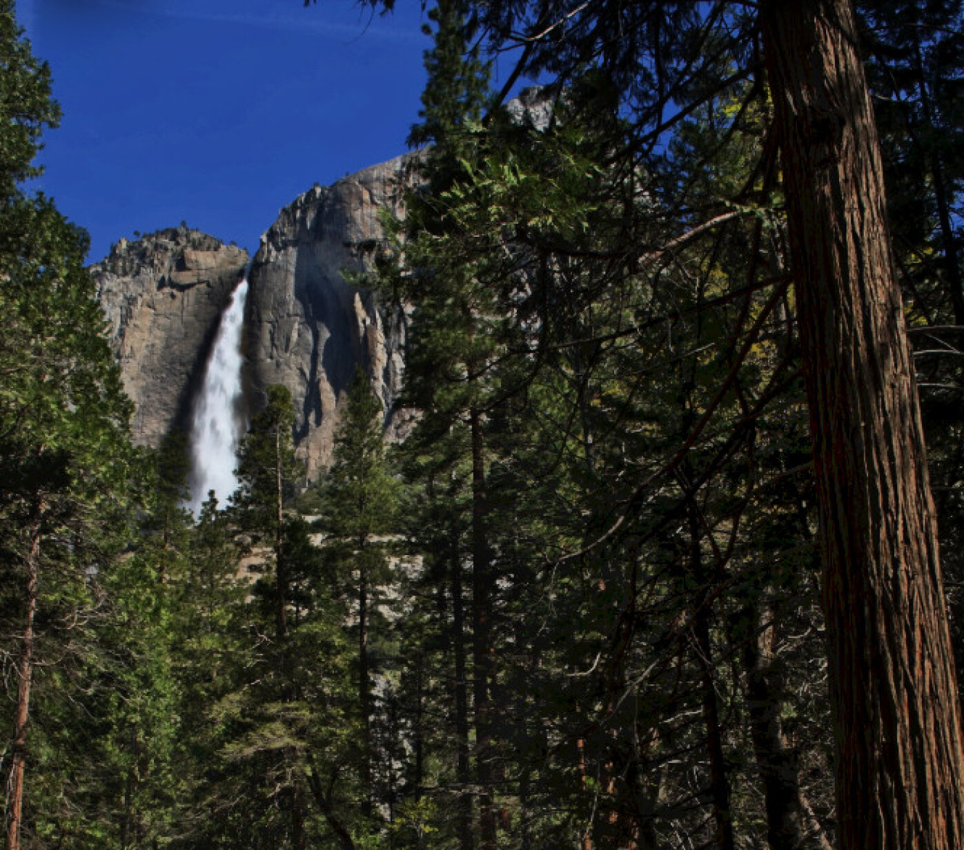
(e) SRIE

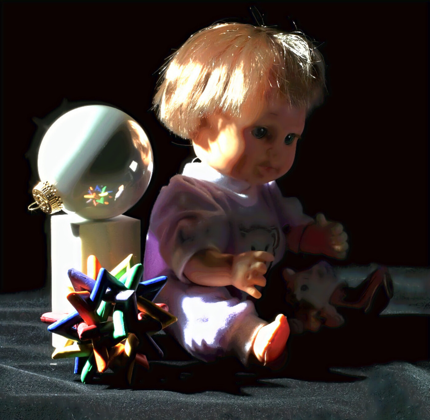
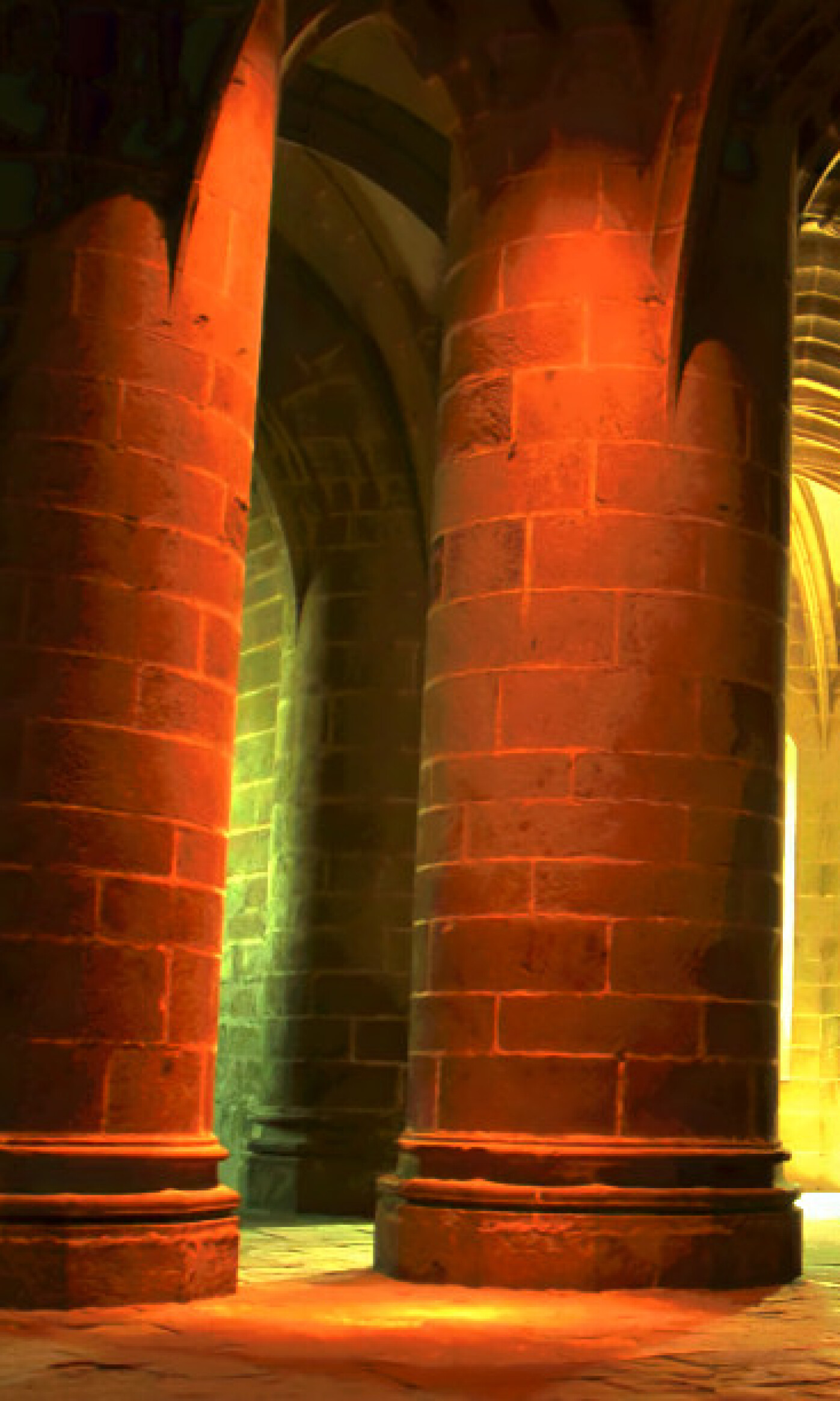
(f) Proposed

Fig. 5: Results of the tested techniques for low-light images synthesized from HDR images.

Fig. 3 shows the visual comparison on two synthetic global low light images. The synthetic images are generated from some normally exposed images from standard benchmark dataset BSD500 [32] by compressing their dynamic ranges by the factor $a^{\gamma_{2}}=1/30,\gamma_{2}/\gamma_{1}=1.3$. Then random gaussian noise $n$($\mu=0,\sigma=0.25$) is added to the images. As shown by the figure, most tested techniques adjust the lightness and contrast successfully, but only the proposed technique can reduce the quantization artifact and restore some missing details.

Fig. 4 shows another experiment on synthetic local low-light images. Dynamic range of the test images is scaled down by the factor $a^{\gamma 2}=1/5,\gamma_{2}/\gamma_{1}=1.5$ [15]. In these test results, there are obviously contours in the results from the methods other than the proposed technique, especially in the relative smooth area such as sky and road. Our method, in comparison, works well for the illumination compensation and quantization residual restoration. The test images in Fig. 5 are synthesized from high dynamic range (HDR) images. In this test case, the proposed algorithm still outperforms the compared algorithms, although it has never been trained using this type of synthetic low-light images.

6.2 Experiments on Real Photographs

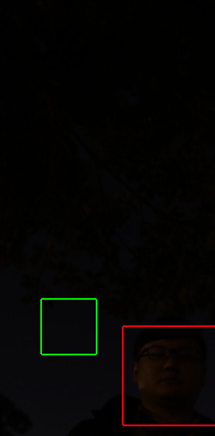
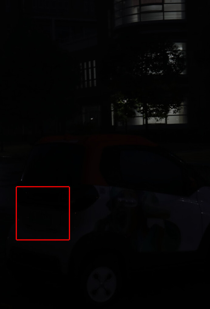
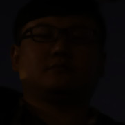
(a) Input

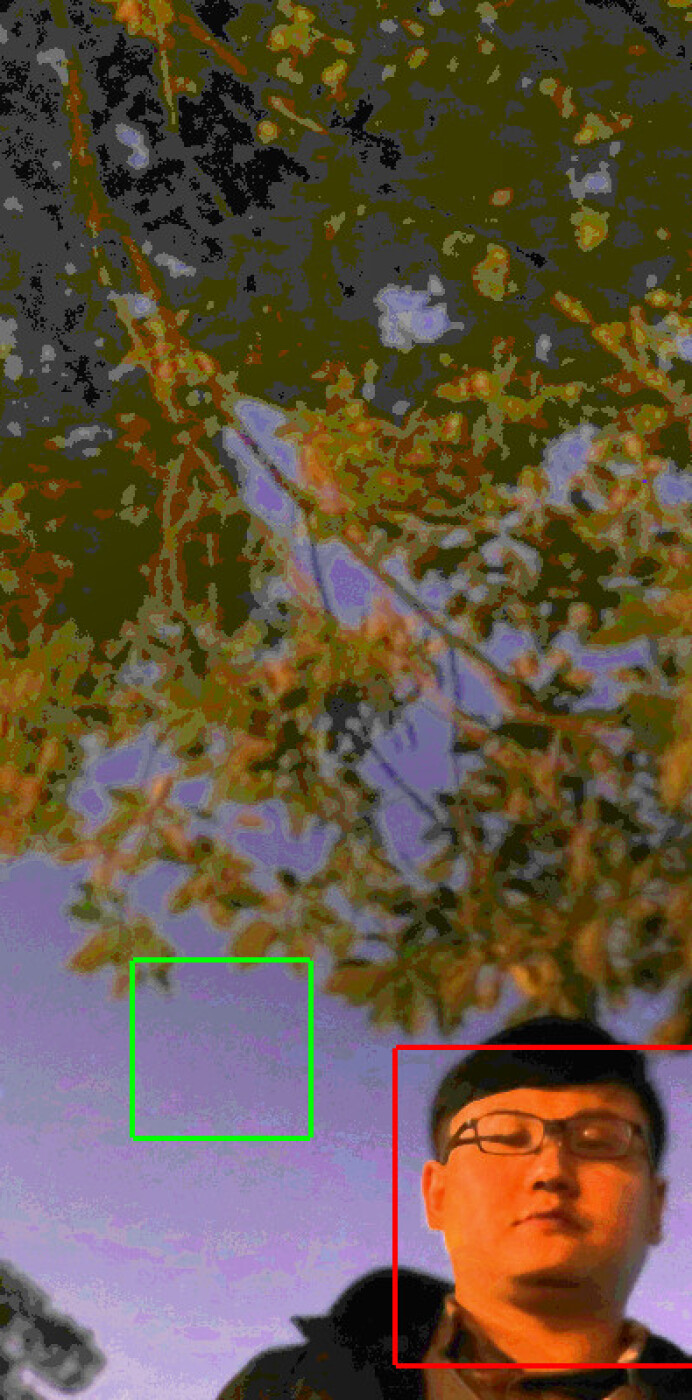
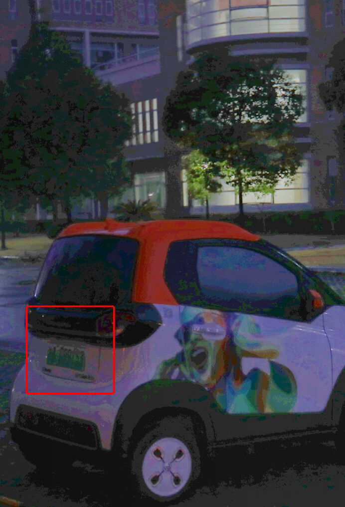
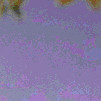
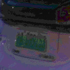
(b) CLAHE

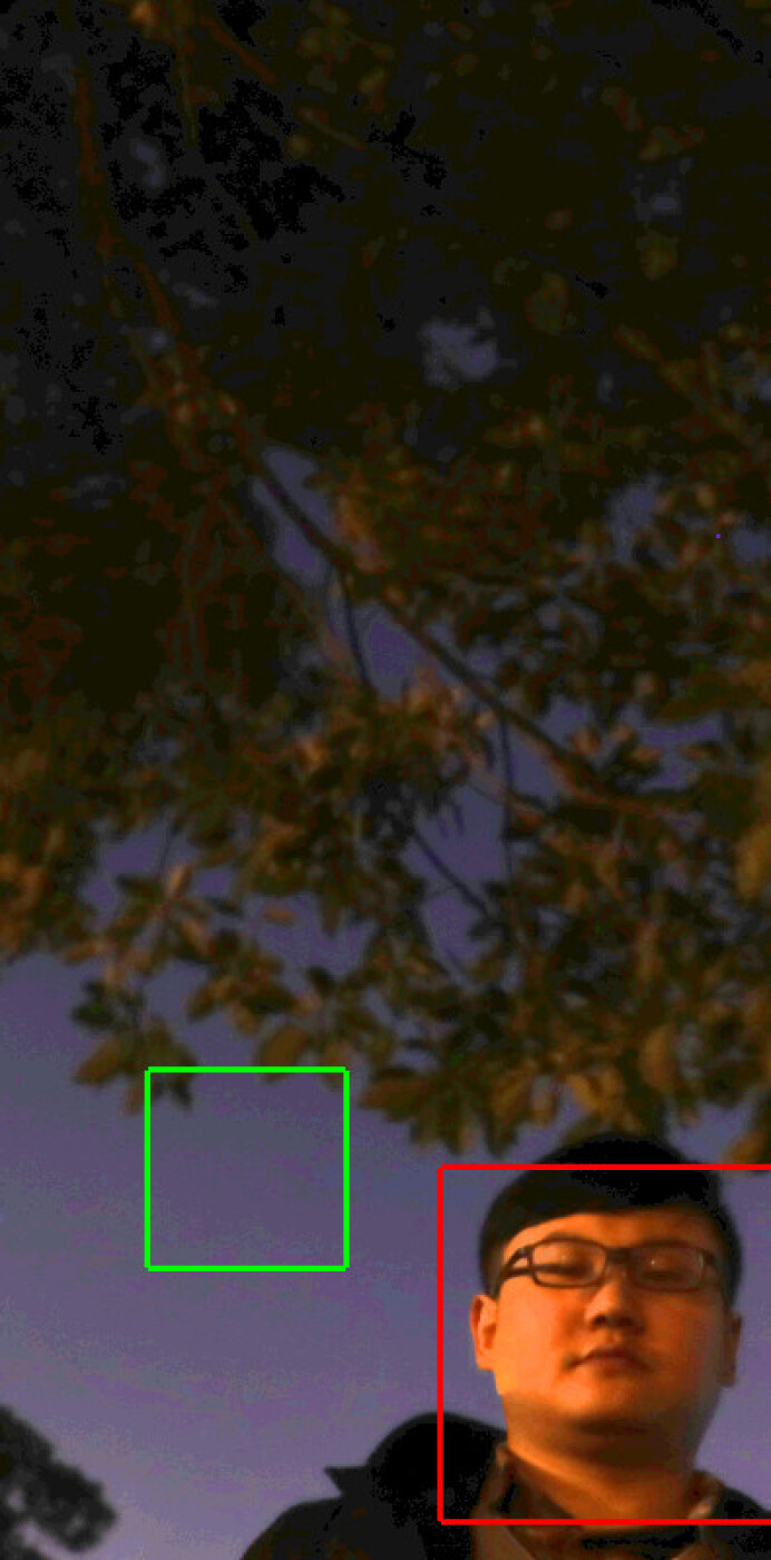
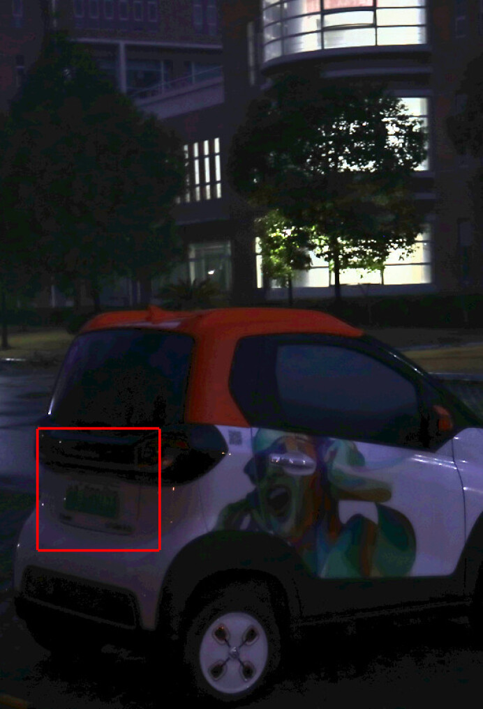
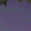
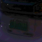
(c) OCTM

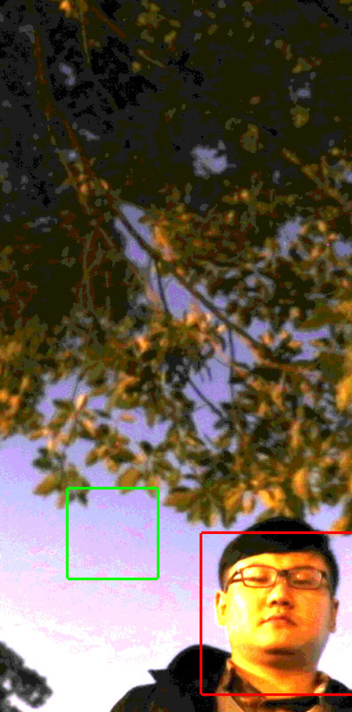
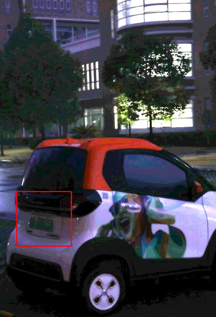
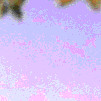
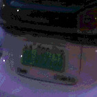
(d) LIME

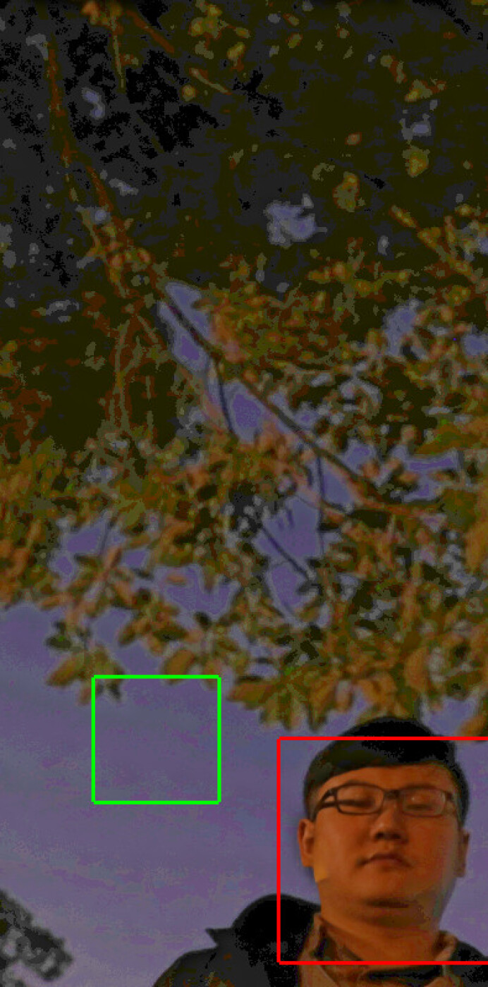
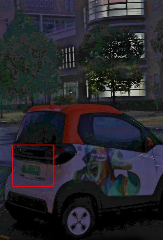
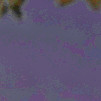
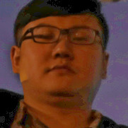
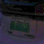
(e) SRIE

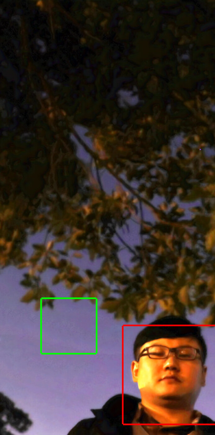
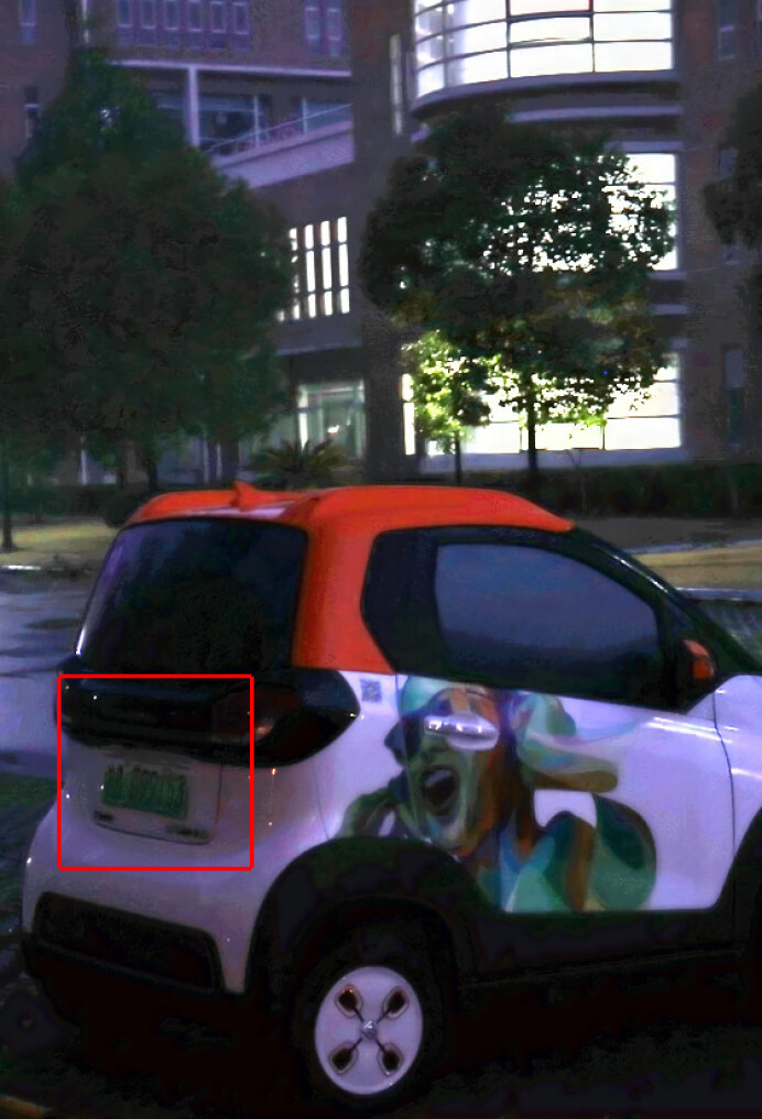
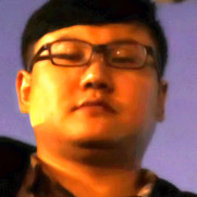
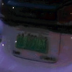
(f) Proposed

Fig. 6: Results of the tested techniques for real photographs.

Experiments on synthetic images demonstrates the superiority of the propose method. For real photographs, the proposed algorithm also works well. Fig. 6 shows some examples of real photographs. Comparing the performance of the five methods, CLAHE can effectively increase the illuminance, but often resulting in low contrast. LIME over-enhances the image. OCTM and SRIE performs better, but their results are not so impressive. For better evaluation, we can see the details in the green and red square. Blocking artifacts appears in all the images enhanced by the four other methods, except for our method. Our method also enhance the human face better than the other techniques and restore the license plate to some extent.

References

- [1] Dan Ciregan, Ueli Meier, and Jürgen Schmidhuber, “Multi-column deep neural networks for image classification,” in Computer Vision and Pattern Recognition (CVPR), 2012 IEEE Conference on. IEEE, 2012, pp. 3642–3649.
- [2] Jianchao Yang, Kai Yu, Yihong Gong, and Thomas Huang, “Linear spatial pyramid matching using sparse coding for image classification,” in Computer Vision and Pattern Recognition, 2009. CVPR 2009. IEEE Conference on. IEEE, 2009, pp. 1794–1801.
- [3] Kaiming He, Xiangyu Zhang, Shaoqing Ren, and Jian Sun, “Deep residual learning for image recognition,” in Proceedings of the IEEE conference on computer vision and pattern recognition, 2016, pp. 770–778.
- [4] Karen Simonyan and Andrew Zisserman, “Very deep convolutional networks for large-scale image recognition,” arXiv preprint arXiv:1409.1556, 2014.
- [5] Alper Yilmaz, Omar Javed, and Mubarak Shah, “Object tracking: A survey,” Acm computing surveys (CSUR), vol. 38, no. 4, pp. 13, 2006.
- [6] Etta D Pisano, Shuquan Zong, Bradley M Hemminger, Marla DeLuca, R Eugene Johnston, Keith Muller, M Patricia Braeuning, and Stephen M Pizer, “Contrast limited adaptive histogram equalization image processing to improve the detection of simulated spiculations in dense mammograms,” Journal of Digital imaging, vol. 11, no. 4, pp. 193–200, 1998.
- [7] Mohammad Abdullah-Al-Wadud, Md Hasanul Kabir, M Ali Akber Dewan, and Oksam Chae, “A dynamic histogram equalization for image contrast enhancement,” IEEE Transactions on Consumer Electronics, vol. 53, no. 2, 2007.
- [8] Turgay Celik and Tardi Tjahjadi, “Contextual and variational contrast enhancement,” IEEE Transactions on Image Processing, vol. 20, no. 12, pp. 3431–3441, 2011.
- [9] Chulwoo Lee, Chul Lee, and Chang-Su Kim, “Contrast enhancement based on layered difference representation of 2d histograms,” IEEE Transactions on Image Processing, vol. 22, no. 12, pp. 5372–5384, 2013.
- [10] Xiaolin Wu, “A linear programming approach for optimal contrast-tone mapping,” IEEE transactions on image processing, vol. 20, no. 5, pp. 1262–1272, 2011.
- [11] Zhenhao Li and Xiaolin Wu, “Contrast enhancement with chromaticity error bound,” in Image Processing (ICIP), 2014 IEEE International Conference on. IEEE, 2014, pp. 4507–4511.
- [12] Edwin H Land, “The retinex theory of color vision,” Scientific American, vol. 237, no. 6, pp. 108–129, 1977.
- [13] Daniel J Jobson, Zia-ur Rahman, and Glenn A Woodell, “Properties and performance of a center/surround retinex,” IEEE transactions on image processing, vol. 6, no. 3, pp. 451–462, 1997.
- [14] Daniel J Jobson, Zia-ur Rahman, and Glenn A Woodell, “A multiscale retinex for bridging the gap between color images and the human observation of scenes,” IEEE Transactions on Image processing, vol. 6, no. 7, pp. 965–976, 1997.
- [15] Xiaojie Guo, Yu Li, and Haibin Ling, “Lime: Low-light image enhancement via illumination map estimation,” IEEE Transactions on Image Processing, vol. 26, no. 2, pp. 982–993, 2017.
- [16] Xueyang Fu, Delu Zeng, Yue Huang, Xiao-Ping Zhang, and Xinghao Ding, “A weighted variational model for simultaneous reflectance and illumination estimation,” in Proceedings of the IEEE Conference on Computer Vision and Pattern Recognition, 2016, pp. 2782–2790.
- [17] Xuan Dong, Guan Wang, Yi Pang, Weixin Li, Jiangtao Wen, Wei Meng, and Yao Lu, “Fast efficient algorithm for enhancement of low lighting video,” in Multimedia and Expo (ICME), 2011 IEEE International Conference on. IEEE, 2011, pp. 1–6.
- [18] Lin Li, Ronggang Wang, Wenmin Wang, and Wen Gao, “A low-light image enhancement method for both denoising and contrast enlarging,” in Image Processing (ICIP), 2015 IEEE International Conference on. IEEE, 2015, pp. 3730–3734.
- [19] Artur Łoza, David R Bull, Paul R Hill, and Alin M Achim, “Automatic contrast enhancement of low-light images based on local statistics of wavelet coefficients,” Digital Signal Processing, vol. 23, no. 6, pp. 1856–1866, 2013.
- [20] Kin Gwn Lore, Adedotun Akintayo, and Soumik Sarkar, “Llnet: A deep autoencoder approach to natural low-light image enhancement,” Pattern Recognition, vol. 61, pp. 650–662, 2017.
- [21] Sergey Ioffe and Christian Szegedy, “Batch normalization: Accelerating deep network training by reducing internal covariate shift,” in International Conference on Machine Learning, 2015, pp. 448–456.
- [22] Alec Radford, Luke Metz, and Soumith Chintala, “Unsupervised representation learning with deep convolutional generative adversarial networks,” arXiv preprint arXiv:1511.06434, 2015.
- [23] Vinod Nair and Geoffrey E Hinton, “Rectified linear units improve restricted boltzmann machines,” in Proceedings of the 27th international conference on machine learning (ICML-10), 2010, pp. 807–814.
- [24] Ian Goodfellow, Jean Pouget-Abadie, Mehdi Mirza, Bing Xu, David Warde-Farley, Sherjil Ozair, Aaron Courville, and Yoshua Bengio, “Generative adversarial nets,” in Advances in neural information processing systems, 2014, pp. 2672–2680.
- [25] Christian Ledig, Lucas Theis, Ferenc Huszár, Jose Caballero, Andrew Cunningham, Alejandro Acosta, Andrew Aitken, Alykhan Tejani, Johannes Totz, Zehan Wang, et al., “Photo-realistic single image super-resolution using a generative adversarial network,” arXiv preprint arXiv:1609.04802, 2016.
- [26] Jun Guo and Hongyang Chao, “One-to-many network for visually pleasing compression artifacts reduction,” arXiv preprint arXiv:1611.04994, 2016.
- [27] Zeev Farbman, Raanan Fattal, Dani Lischinski, and Richard Szeliski, “Edge-preserving decompositions for multi-scale tone and detail manipulation,” ACM Transactions on Graphics, vol. 27, no. 3, pp. 67:1–67:10, 2008.
- [28] Raanan Fattal, Dani Lischinski, and Michael Werman, “Gradient domain high dynamic range compression,” ACM Transactions on Graphics, vol. 21, no. 3, pp. 249–256, 2002.
- [29] Sylvain Paris, Samuel W. Hasinoff, and Jan Kautz, “Local laplacian filters: Edge-aware image processing with a laplacian pyramid,” ACM Transactions on Graphics, vol. 30, no. 4, pp. 68:1–68:12, 2011.
- [30] Ziaur Rahman and Glenn A. Woodell, “Retinex processing for automatic image enhancement,” Journal of Electronic Imaging, vol. 13, pp. 100–110, 2004.
- [31] Erik Reinhard, Michael Stark, Peter Shirley, and James Ferwerda, “Photographic tone reproduction for digital images,” ACM Transactions on Graphics, vol. 21, no. 3, pp. 267–276, 2002.
- [32] David Martin, Charless Fowlkes, Doron Tal, and Jitendra Malik, “A database of human segmented natural images and its application to evaluating segmentation algorithms and measuring ecological statistics,” in Computer Vision, 2001. ICCV 2001. Proceedings. Eighth IEEE International Conference on. IEEE, 2001, vol. 2, pp. 416–423.