SED constraints on the highest-$z$ blazar jet: QSO J0906$+$6930

Abstract

We report on Gemini, NuSTAR and 8-year Fermi observations of the most distant blazar QSO J0906$+$6930 ($z=5.48$). We construct a broadband spectral energy distribution (SED) and model the SED using a synchro-Compton model. The measurements find a $\sim 4\times 10^{9}M_{\odot}$ mass for the black hole and a spectral break at $\sim$4 keV in the combined fit of the new NuSTAR and archival Chandra data. The SED fitting constrains the bulk Doppler factor $\delta$ of the jet to $9^{+2.5}_{-3}$ for QSO J0906$+$6930. Similar, but weaker $\delta$ constraints are derived from SED modeling of the three other claimed $z>5$ blazars. Together, these extrapolate to $\sim 620$ similar sources, fully 20% of the optically bright, high mass AGN expected at $5<z<5.5$. This has interesting implications for the early growth of massive black holes.

1. Introduction

The existence of massive black holes (BH) at $z>5$ is well known, via optical/IR surveys for bright quasars (e.g. Fan et al., 2001; Mortlock et al., 2011). The most massive high-redshift sources present a puzzle; it is challenging to grow a stellar mass seed black hole to $>10^{9}M_{\odot}$ levels in the limited age of the universe. By inferring the cosmic density of quasars we can probe viable growth scenarios (Berti & Volonteri, 2008).

Super-massive BHs can grow by merging or accretion. Merging BHs may have random spin orientation and thus modest final BH angular momentum. Disk accretion growth increases the angular momentum along with the mass, but the accretion energy yield also increases with the spin, so that Eddington-limited mass growth rates would decrease. Thus large accretion-fed masses may be particularly difficult to reach at early times. The so-called blazars are active galaxies dominated by the two-humped (synchrotron + Compton) spectral energy distribution (SED) of relativistic jet emission. As such they are bright microwave-IR (synchrotron) and gamma-ray (Compton) sources. Moreover it is believed that this large jet power can be traced to efficient extraction of rotational energy of a black hole with spin $a$ (Blandford & Znajek, 1977). Thus searches for blazar sources at high $z$ (see also Ackermann et al., 2017) may be a particularly interesting probe of the accretion-dominated growth channel.

Inspired by early EGRET detections, radio/optical surveys have indeed found many blazars (Sowards-Emmerd et al., 2005; Healey et al., 2007); most have now been detected by Fermi and have led to better understanding of the evolution of this massive, jet-dominated BH population (Ajello et al., 2014). But these objects are largely at relatively modest $z<3$ redshifts. To date only four blazars at $z>5$ have been reported in the literature (i.e., QSO J0906$+$6930, B2 1023+25, SDSS J114657.79+403708.6, SDSS J0131$-$0321; Romani et al., 2004; Sbarrato et al., 2013; Ghisellini et al., 2014, 2015). Although we do not have formal evaluation of the completeness of this sample, the sources are identified from wide area radio surveys (§3), and therefore, the study of these objects can help us understand the high redshift blazar population.

This small sample size may be natural since the emission is dominated by the relativistic jet, which is highly beamed. For bulk Lorentz factor $\Gamma_{\rm D}$, each blazar detection represents $\sim 2\Gamma_{\rm D}^{2}$ similar sources beamed away from Earth (for a more detailed estimate see §4). Thus population inferences require careful extrapolation of these few detected sources with good estimates of the viewing angle ($\theta_{\rm V}$) and bulk Doppler factor $\delta=1/[\Gamma_{\rm D}(1-\beta\mathrm{cos}\theta_{\rm V})]$, where $\beta=\sqrt{1-1/\Gamma_{\rm D}^{2}}$. These can be extracted by measuring the SED using the different dependencies of the synchrotron ($\nu_{sy,pk}^{obs}\propto\delta$), self-Compton ($\nu_{ssc,pk}^{obs}\propto\delta$, SSC) and external Compton ($\nu_{pk}^{obs}\propto\delta^{2}$, EC) components. Adequately defining these emission components is, however, particularly challenging, since the known $z>5$ blazars lack Fermi detections, and their synchrotron emission peak seems to fall in the millimeter wavelength range. We therefore rely on hard X-ray measurements and GeV upper limits to constrain $\delta$.

The most distant ($z=5.48$) blazar is the radio bright $S_{8.4GHz}\sim 140$ mJy GB6 0906+6930 (hereafter Q0906). It was actually found coincident with a low-significance ($1.5\sigma$ at one epoch) excess of EGRET gamma rays. Romani et al. (2004) and Romani (2006) measured the SED of Q0906 in the radio to X-ray band and generated models that could allow the EGRET detection. These implied $\Gamma_{\rm D}\sim 13$, but the SED peaks were not well constrained. New Fermi upper limits presented here imply substantially lower average gamma-ray flux. Given that large $\Gamma_{\rm D}$, and similar values inferred for other $z>5$ blazars would suggest large accretion-fed populations, improved constraints on the blazar properties are needed.

Here, we report on Gemini, NuSTAR and 8-yr Fermi-LAT observations and jet properties inferred by SED modeling. We describe the broadband data we collect in Section 2 and report the data analysis results and SED modeling in Section 3. We then discuss implications of our studies and conclude in Section 4. We use $H_{0}=70\rm\ km\ s^{-1},\Omega_{m}=0.3$ and $\Omega_{\Lambda}=0.7$ throughout (Komatsu et al., 2011).

2. Observation Data and Basic Processing

In the IR band, Q0906 was observed with the Gemini-N GNIRS on December 3, 2015 (program GN-2015B-FT-22), using the short $0.15^{\prime\prime}$/pixel camera, the 32l/mm grating and the $0.3^{\prime\prime}$ slit at the average parallactic angle. This provides coverage from 0.88–2.5$\mu m$ in orders 3 through 8 with resolving power $R\sim 1400$. Relative calibration was provided by $4\times 2$ s spectroscopic integrations (ABBA pattern) of the flux standard HIP43266. Although the standard was acquired with a direct $H$ image, this was saturated, so we could not measure the slit losses to establish an absolute flux scale. Next Q0906 was observed, starting with three direct images through the $H$ filter, each comprised of $12\times 3$ s co-added. The stacked image FWHM was $0.41^{\prime\prime}$. We then obtained 12 spectroscopic exposures of 300 s, dithering along the slit in an ABBA pattern. The first two exposures suffered contamination from a bright persistence signal, while the last two had a severely increased background from morning twilight. This left 8 useful exposures, totaling 2400 s.

We also observed Q0906 with the NuSTAR observatory (Harrison et al., 2013) between MJD 57732 (2016-12-10 UTC) and 57734 (2016-12-11 UTC) with 75 ks total exposure (LIVETIME) to collect a hard X-ray spectrum in the 3–79 keV band. For this observation, the NuSTAR Science Operation Center (SOC) reported slightly elevated background rates around South Atlantic Anomaly (SAA) passage and recommended that we use more strict filters. The data are downloaded from the NuSTAR archive and are processed with the nupipeline tool integrated in HEASOFT 6.19 along with the NuSTAR CALDB (release 20160706) with the strict filters suggested by the SOC.

In the gamma-ray band, we use the Pass-8 reprocessed Fermi-LAT data (Atwood et al., 2009, 2013) collected between 2008 August 04 and 2016 November 28 UTC. We processed the data with the Fermi-LAT Science Tools v10r0p5 along with P8R2_V6 instrument response functions, and selected source class events with Front/Back event type in an $R=10^{\circ}$ aperture in the 100 MeV–300 GeV band. We further employed standard $<90^{\circ}$ zenith angle and $52^{\circ}$ rocking angle cuts.

Broadband coverage helps us pin down the SED peaks and so we use archival radio, IR, optical and soft X-ray data. For the IR data, we take the measurements from the WISE and the Spitzer catalogs. For the radio and the optical data, we use the measurements reported by Romani (2006). In the soft X-ray band ($<$10 keV), we reanalyze the archival 30-ks Chandra data (Romani, 2006) and the Swift/XRT data (11 exposures). The Chandra data are reprocessed with chandra_repro of CIAO 4.8 using CALDB 4.7.2, and the Swift data are processed with xrtpipeline in HEASOFT 6.19 with the HEASARC remote CALDB. Note that the latest Swift exposure is contemporaneous with the NuSTAR observation; comparison with other Swift epochs confirm that the blazar was in an average state, suitable for comparison with non-simultaneous multiwavelength observations.

3. Data Analysis and Modeling

3.1. Gemini Data Analysis

The GNIRS spectra were reduced with scripts from the Gemini 1.13 package, including removal of pattern noise, flat fielding, rectification, wavelength calibration and fluxing with the standard spectrum. The orders were combined into a single spectrum, which is smoothed and plotted in Figure 1. The unsmoothed S/N/pixel peaks at $\sim 6$ in the middle of the orders. The J/H (1.35–1.45$\mu m$) and H/K (1.82–1.91$\mu m$) gaps, with low atmospheric transmission, are particularly noisy and are plotted in red. We also show the HET G1 spectrum of Romani et al. (2004). With unknown differential slit losses between the standard and target exposures, we elect to normalize to the direct imaging fluxes measured by PanSTARRS. We integrate the HET G1 spectrum over $0.818-0.922\mu m$ and scale to the magnitude $z=19.83\pm 0.05$, while an integration of the GNIRS spectrum over $0.918-1.001\mu m$ is scaled to the $y=19.54\pm 0.09$ image flux.

We examined our direct $H$ image where the quasar is well detected. The GNIRS H-band spectrum has a flux of $5.9\times 10^{-18}{\rm erg/cm^{2}/s/\AA}$. No other source is detected in the GNIRS ‘keyhole’ field, placing an upper limit of $3.5\times 10^{-19}{\rm erg/cm^{2}/s/\AA}$ on any source within $\sim 3^{\prime\prime}$ of the quasar (limited by the nearby edge of the keyhole field of view). This provides a modest limit of $L<2.3L_{\ast}$ on the luminosity of any intervening galaxy associated with the strong Mg II absorption system at $z=1.849$ (Romani, 2006). No nearby sources are seen in the PanSTARRS images.

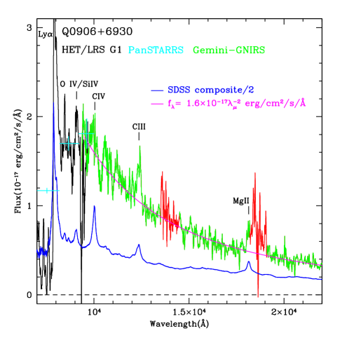
Figure 1.— The near-IR spectrum of Q0906, with the HET G1 (black) and GNIRS (green) spectra. These are matched to imaging PanSTARRS fluxes ($i$, $z$ and $y$ shown as red error flags). In the GNIRS spectrum, regions between the near-IR windows have very low S/N and are plotted in red. A redshifted composite SDSS QSO spectrum is shown in blue, scaled down by $2\times$ for visibility. A simple power-law approximation to the GNIRS continuum is plotted in magenta. Strong UV resonance lines are marked. C IV is weak and appears affected by poor continuum fluxing. Mg II is partly lost to atmospheric absorption.

The IR spectrum has a continuum approximated by $f_{\lambda}=1.6\times 10^{-17}\lambda_{\mu}^{-2}{\rm erg/cm^{2}/s/\AA}$. In Figure 1 we also plot the SDSS composite QSO spectrum of Vanden Berk et al. (2001), redshifted to $z=5.48$ and scaled down by $\sim 2\times$. We are particularly interested in the UV emission lines shifted to the IR. C IV (1550) is rather poorly detected, being absorbed by a strong (rest frame EW=0.8Å) associated doublet at $z=5.469$ and being flanked by large continuum oscillations, possibly due to poor fluxing. Its overall weakness is likely a consequence of the large QSO luminosity (Baldwin effect). C III (1909) is well detected, while Mg II (2800) is at the edge of the H-band with the red half of the line lost to atmospheric absorption. This is unfortunate, since we can use neither of the standard calibrated species (C IV, Mg II) for a virial mass estimate. For the C III line we measure a Gaussian FWHM=$6200\pm 400$ km/s. The left half of the Mg II line provides a line width estimate FWHM$\approx 6000$ km/s. For C IV the poorly defined continuum prevents any meaningful line width estimate. In Romani et al. (2004) the O IV/S IV line was estimated to have FWHM=$5000\pm 500$ km/s. If we assume a line width of 6000 km/s then, measuring the standard continuum luminosity for C IV ($\lambda L_{\lambda}{1350}=5.4\times 10^{46}{\rm erg/s}$) gives log$M_{\bullet}=9.66$ (McLure & Dunlop, 2004) while Mg II ($\lambda L_{\lambda}{3000}=2.7\times 10^{46}{\rm erg/s}$) gives log$M_{\bullet}=9.57$. These give an average inferred BH mass $M_{\bullet}=4.2\times 10^{9}M_{\odot}$, subject to the usual systematic uncertainties as well as the errors from the poor spectral line measurements. Still, these IR spectra provide a useful mass estimate and show the flattening of the IR SED bump toward a peak at $\sim 0.9\mu m$.

3.2. X-ray Data Analysis

Because blazars are often variable in all wavebands, combining data taken in different epochs needs to be done with care. We therefore first checked for time variability of the X-ray flux using Swift archive data, which have observations spanning 11 years (2006 Jan. 20–2016 Dec. 10). We constructed a long-term light curve using circles with $R=20^{\prime\prime}$ and $R=40^{\prime\prime}$ for source and background extraction, respectively. A total of $76\pm 11$ background-subtracted events were detected over the integrated 43 ks exposure (summed over the 11-yr observations). All epochs have count rates within 60% of the average and there is no evidence for spectral variability; within the statistic-limited sensitivity, the light curve is consistent with being constant. In particular, the Swift observation contemporaneous with the NuSTAR observation, has a count rate consistent with the light curve average and with the count rate expected from the measured Chandra spectrum (see below). Therefore, we conclude that the Q0906 variability is small, that it was in a typical state during the NuSTAR exposure, and that we can reasonably combine non-contemporaneous observations in forming the SED.

For X-ray spectral properties, we first reanalyzed the Chandra data. Source events were extracted from a $R=2^{\prime\prime}$ circular aperture and background from an annular region with $R_{\rm in}=5^{\prime\prime}$ and $R_{\rm out}=10^{\prime\prime}$ centered at the source position. Response files are calculated using the specextract tool of CIAO. For the absorption model, we use $\tt wilm$ abundance (Wilms et al., 2000) and $\tt verner$ cross section (Verner et al., 1996). We group the spectrum to have at least 20 counts per bin and fit the spectrum with an absorbed power-law model (PL) in XSPEC. The spectral parameters are consistent with previous measurements (Romani, 2006).

The 11 Swift observations were separately analyzed. We used a $R=20^{\prime\prime}$ circular region for source spectra. A source-free nearby $R=40^{\prime\prime}$ region was used for background extraction. The ancillary response files (ARFs) were produced with the xrtmkarf tool correcting for the exposure, and we used pre-generated redistribution matrix files (RMFs). After this, we find that individual Swift spectra do not have enough events for a meaningful spectral analysis. We therefore combine all the spectra with the addspec tool of HEASOFT. We grouped the combined spectrum to have at least 20 counts per spectral bin, and fit the spectrum with an absorbed power-law model holding $N_{\rm H}$ fixed at the Chandra-measured value. Employing different statistics (e.g., lstat in XSPEC) or different binning does not change the parameters significantly. The results are also consistent with the Chandra values above (Table 1).

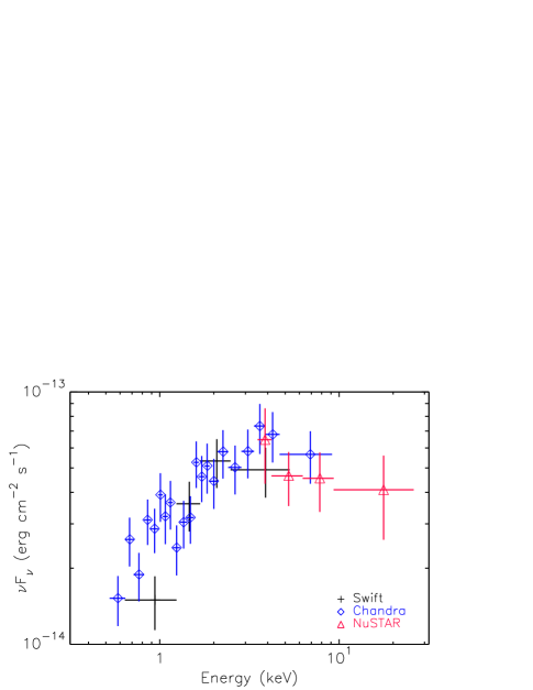
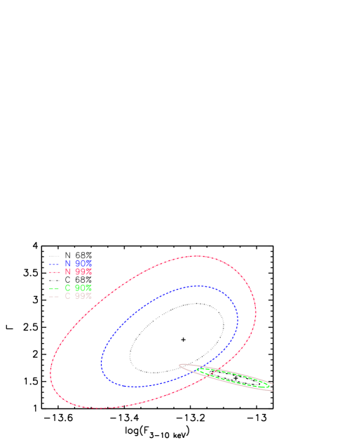
Figure 2.— Left: X-ray SED of Q0906 measured with Swift, Chandra and NuSTAR. Right: confidence contours in the $\mathrm{l}ogF$-$\Gamma$ space for the NuSTAR and Chandra fits. 68%, 90%, and 99% contours corresponding to $\Delta\chi^{2}=$2.3, 4.61 and 9.21, respectively, are shown in lines.

For the NuSTAR data analysis, we used $R=30^{\prime\prime}$ and $R=60^{\prime\prime}$ regions for the source and the background extraction, respectively. The corresponding response files were calculated with the nuproduct tool. Q0906 was surprisingly faint, yielding only 120$\pm$20 source events in the 3–20 keV band while we expected 260 counts if the Chandra-measured power-law spectrum extends to higher energies. Keeping this in mind, we grouped the spectra to have at least 20 events per spectral bin and fit the NuSTAR spectra with a simple power-law model. We find that the measured 3–20 keV spectrum is softer than the soft band determination (Table 1), having an index $\Gamma=2.3\pm 0.4$ (Figure 2 left). For such a faint source, the fit parameters might be sensitive to the fit statistic or background selection. We therefore varied both; we used three different $R=60^{\prime\prime}$ background regions, and fit the data using $l$ statistic or $\chi^{2}$ statistic. None of these tests gave significant changes to the measured parameters.

The low NuSTAR count rate may imply a softer spectrum at higher energies. So we checked to see if the best-fit NuSTAR parameters are consistent with the Chandra-measured values using the steppar command of XSPEC. This provides confidence contours for the NuSTAR parameters and shows that the Chandra values lie outside the 99% contour (Figure 2 right), although including the Chandra parameter uncertainty, there is some overlap.

Table 1X-ray spectral fit results for Q0906

Individual fits
Instrument	Model	$\Gamma_{\rm s}$	$E_{\rm b}$	$\Gamma_{\rm h}$	$F$	$\chi^{2}$/dof
			(keV)
S	PL	$1.32\pm 0.21$	$\cdots$	$\cdots$	$1.5\pm 0.3$	4/4
C	PL	$1.56\pm 0.14$	$\cdots$	$\cdots$	$1.5\pm 0.1$	14/18
N	PL	$2.27\pm 0.41$	$\cdots$	$\cdots$	$0.6\pm 0.1$	8/11
Joint fits
S+C+N	PL	$1.55\pm 0.07$	$\cdots$	$\cdots$	$0.46\pm 0.10$	30/34
S+C+N	BPL	$1.44\pm 0.10$	$3.8\pm 1.0$	$2.33\pm 0.42$	$0.60\pm 0.13$	25/32

Notes. $N_{\rm H}$ is measured to be $8\times 10^{20}\rm\ cm^{-2}$ with the Chandra fit and held fixed at this value for the other fits. Instruments are Swift (S), Chandra (C), and NuSTAR (N).
^aPower law index $\Gamma_{\rm s}$. If broken at $E_{\rm b}$ hard index is $\Gamma_{\rm h}$.
^bAbsorption-corrected 0.5 keV–10 keV flux in units of $10^{-13}\rm\ erg\ cm^{-2}\ s^{-1}$ for Swift and Chandra fits and 3 keV–10 keV flux for NuSTAR and joint fits.

A joint XSPEC fit of the Chandra, Swift and NuSTAR data to a simple power law with free cross-normalization yields $\Gamma=1.55\pm 0.07$ consistent with that measured with Chandra alone. This is evidently due to the Chandra count dominance. The fit tension is revealed in the anomalously large cross-normalization factor $1.9\pm 0.6$ with Chandra. If we fit the data sets with an absorbed broken power law (BPL), the cross-normalization factor for Chandra becomes $1.2\pm 0.3$, consistent with the nominal calibration offset of $\sim$10% (Madsen et al., 2015). The best-fit parameters for this broken power-law model are $\Gamma_{\rm s}=1.44\pm 0.10$, $E_{\rm break}=3.8\pm 1.0$ keV, and $\Gamma_{\rm h}=2.3\pm 0.4$ (see Table 1). The improvement of these broken power-law fits is modest, but the improved relative normalization lends confidence that this is a better model. Note that similar spectral breaks have been seen in other blazars (Hayashida et al., 2015; Tagliaferri et al., 2015; Sbarrato et al., 2016; Paliya et al., 2016) and were variable in some cases.

Although we do not significantly detect the source above $\sim$30 keV, NuSTAR can still be used to derive an upper limit that gives a useful constraint on the SED Compton peak. Fixing the index at the $\Gamma_{\rm h}=2.33$ of the broken power-law fit, we use the steppar tool of XSPEC to scan the normalization while comparing with the 20–79 keV NuSTAR data. Finding the value at which $\Delta\chi^{2}$ increases by 2.71, we establish a 95% flux upper limit of $2.4\times 10^{-13}\rm\ erg\ cm^{-2}\ s^{-1}$. The SED is shown in Figure 3 (top left).

3.3. Fermi-LAT Data Analysis

We next derived a spectrum from 8-yr years of 100 MeV–300 GeV Fermi-LAT ‘Pass8’ data using binned likelihood analysis. We fit the spectrum to a power-law model using the pyLikelihood package provided along with the Science Tools. Because Q0906 is not in the 3FGL catalog (Acero et al., 2015), we added it to the 3FGL XML model assuming a power-law spectrum. We then fit the data, varying parameters for Q0906, nearby bright sources, the diffuse emission (gll_iem_v06.fits; Acero et al., 2016) and the isotropic emission (iso_P8R2_SOURCE_V6_v06.txt; Ackermann et al., 2015) in the 100 MeV–300 GeV band. Q0906 is not detected, having a mission-averaged test statistic (TS) value of $<1$. We also varied the number of nearby sources to fit and the aperture size (Region of interest, RoI $R=5^{\circ}$ and $R=15^{\circ}$), and found that the result does not change. We therefore report the 95% flux upper limit for Q0906 of $6\times 10^{-10}\rm\ ph\ cm^{-2}\ s^{-1}$ in the 100 MeV–300 GeV band assuming a typical $\Gamma=2$ photon index derived using the UpperLimits.py script, which scans the power-law amplitude to find the value for which the loglikelihood ($-\mathrm{l}og\mathcal{L}$) increases by 1.35 from the minimum value.

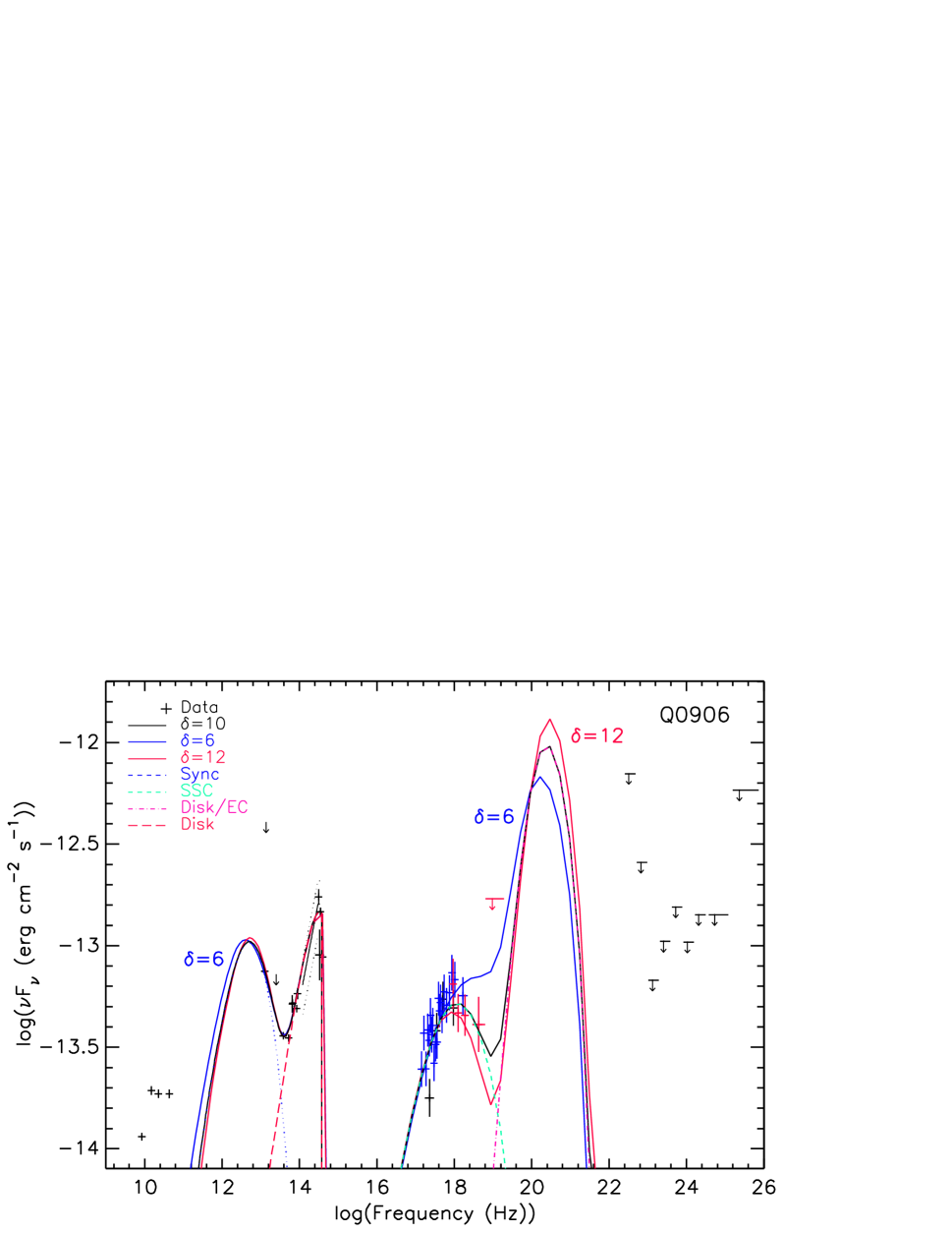
Figure 3.— The broadband SED of Q0906 and the synchro-Compton models. The model parameters are adjusted to match the SEDs and shown in Table 2. We also show two models with a lower (blue) and the maximum (red) $\delta$: 6 and 12 for Q0906. We show the X-ray data in color for clarity: black for Swift, blue for Chandra and red for NuSTAR.

Next, since the strongest SED constraints may be energy dependent, we derive the LAT SED of Q0906 in nine energy bands. For this, we assumed a power-law spectrum across each band with $\Gamma=2$ and fit the amplitude of the power-law model in individual energy bands. As expected, the source was not detected (TS$<$9) in any of the energy bands, and we provide the 95% flux upper limits. These gamma-ray flux limits shown in Figure 3 (top left). We note that the upper limits are not very sensitive to the assumed power-law index.

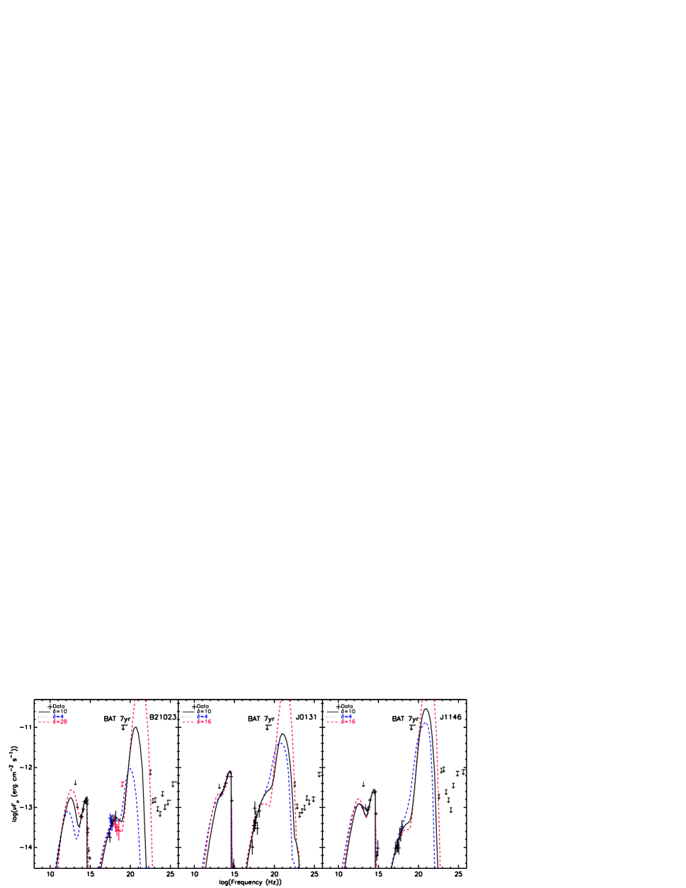
Figure 4.— Broadband SEDs and the synchro-Compton models for B2 1023+25 (left), SDSS J013127.34$-$032100.1 (middle), and SDSS J114657.79+403708.6 (right). Models with a lower (blue dotted) and the maximum (red dashed) $\delta$, 4 and 28 for B2 1023, 4 and 16 for J0131, and 4 and 16 for J1146 are also shown. For B2 1023+25, the same models for Q0906 work well but here we show a different set of models with lower-$B$ and larger EC emission; this is possible for B2 1023 because the synchrotron SED is not constrained with the data.

Finally, we check to see if the source is variable in gamma rays. In particular, if there had been a large flare, the source might have had higher significance during a restricted period. For this, we generated a light curve using 1-Ms time bins and performed likelihood analysis to derive 100 MeV–300 GeV flux in each time bin. In the likelihood analysis, we vary the amplitudes of Q0906 and nearby bright and variable sources (with the variability index greater than 100 in the 3FGL catalog). The test statistics for Q0906 is less than 9 in most of the time intervals. There is one time interval in which the detection significance is higher (TS$\approx$12, MJD 56396–56407). Although this is the highest value we get in our analysis, the probability of having such a value or greater in 263 trials (time bins) is 14%, implying that this is not sufficient to claim a detection.

3.4. Broadband SED Modeling

Combining the new and archival data (Sections 3.2 and 3.3) we construct the broadband SED for Q0906 in Figure 3. From the SED peak frequencies, we can derive rough constraints on the bulk Doppler factor. In synchro-Compton models, the low energy hump in the SED is produced by synchrotron radiation. Thermal emission from the disk provides an intermediate peak at $\nu_{BB,pk}$ in the IR-optical band (Shakura & Sunyaev, 1973) for Q0906. X-ray emission is produced by self-Compton scattering of the synchrotron emission, and an external Compton component from up-scattered disk photons will produce a hump in the MeV band (see Figure 3). The SED peak frequencies are related by $\nu_{sy,pk}^{obs}\approx\frac{\nu_{sy,pk}\delta}{1+z}$ (Synchrotron, with $\nu_{sy,pk}\approx 3.7\times 10^{6}\gamma_{e}^{2}B$), $\nu_{ssc,pk}^{obs}\approx\frac{\nu_{sy,pk}\delta\gamma_{e}^{2}}{1+z}=\gamma_{e}^{2}\nu_{sy,pk}^{obs}$ (self-Compton) and $\nu_{EC,pk}^{obs}\approx\frac{\nu_{BB,pk}\delta^{2}\gamma_{e}^{2}}{1+z}=\delta^{2}\gamma_{e}^{2}\nu_{BB,pk}^{obs}$ (external inverse Compton). With incomplete coverage, the peak frequencies are uncertain, but from the SED shape we estimate $\nu_{sy,pk}^{obs}\approx 4\times 10^{12}$ Hz, $\nu_{BB,pk}^{obs}\approx 3\times 10^{14}$ Hz, $\nu_{ssc,pk}^{obs}\approx 10^{18}$ Hz, and $2\times 10^{19}\rm\ Hz<\nu_{EC,pk}^{obs}<10^{22}\rm\ Hz$. From visual estimates of the SED peak positions and the frequency scaling above we see that $\gamma_{e}\approx(\nu_{ssc,pk}^{obs}/\nu_{sy,pk}^{obs})^{1/2}\approx 500$ and $\delta\approx(\nu_{EC,pk}^{obs}/\nu_{BB,pk}^{obs})^{1/2}/\gamma_{e}\approx 0.6-13$.

We can make better estimates by comparing the data with detailed SED models. We use the synchro-self-Compton model developed by Boettcher et al. (1997) to describe the broadband blazar SED. This model assumes a continuous injection into a $e^{+}/e^{-}$ blob at the jet base (at a height $h$=0.03 pc from the BH) and evolves the blob over an interval of $10^{7}$ s following radiative losses. The properties of the blob (injection spectrum, bulk Doppler factor, magnetic field strength, and so forth) are prescribed, and the code delivers the integrated emission spectrum. As above, we assume that the low-energy $\stackrel{{\scriptstyle<}}{{{}_{\sim}}}10^{13}$ Hz emission is produced by synchrotron radiation. The radio points are, as usual, well above the expectation of the core synchrotron component as these represent the late time emission of the blobs after they flow to large (VLBI-scale) radii (e.g., Collmar et al., 2010). The $\sim 10^{14}$ Hz SED is the disk blackbody emission, absorbed to the blue by the intragalactic Lyman-$\alpha$ forest. Two processes contribute to the X-ray emission: synchro-self-Compton radiation and external Compton up-scattering of the disk photons. As one moves to higher X-ray energies, the external Compton from the higher-frequency disk photons should become increasingly important. Since larger $\delta$ shifts the EC peak to higher frequency, its contribution to the X-ray band is very sensitive to this factor. For small $\delta$ we expect the sharp rise to the EC peak to enter the NuSTAR band; for larger $\delta$ we will see the falling spectrum above the isolated $\nu_{ssc,pk}^{obs}$ peak.

We compute the disk blackbody emission with a Shakura-Sunyaev (Shakura & Sunyaev, 1973) model. In Figure 1, we appear to detect a continuum flattening above $\sim 3\times 10^{14}$ Hz. However, the onset of Lyman-$\alpha$ forest absorption at $3.8\times 10^{14}$ Hz precludes detailed measurement of the thermal peak. We therefore used the viral BH mass estimate $M_{\bullet}=4.2\times 10^{9}M_{\odot}$ (Section 3.2) and adjust $L_{\rm disk}$ to match the disk IR flux (e.g., Calderone et al., 2013). The optical-IR SED matches that of a Shakura-Sunyaev disk for disk luminosity $L_{\rm disk}=2.4\times 10^{47}\rm\ erg\ s^{-1}$. This is $\sim 0.4L_{Edd}$, suggesting that the thin disk approximation is adequate. The virial estimates are uncertain and smaller BH masses adjust the disk luminosity: e.g., $M_{\bullet}=3\times 10^{9}M_{\odot}$ implies $L_{\rm disk}=2.6\times 10^{47}\rm\ erg\ s^{-1}$. However, this uncertainty induces rather small ranges in the other model parameters, so we neglect it below.

For blazars, the synchrotron-producing electron spectrum typically has an index $p_{1}\approx 2$; here we use $p_{1}=1.8$ for the best SED match. This spectrum ranges from minimum $\gamma_{\rm e,min}$ to maximum $\gamma_{\rm e,max}$. These values and the magnetic field strength $B$ are adjusted to match the shapes and the amplitudes of the synchrotron and the X-ray SEDs. Given the large number of parameters, SED data alone are insufficient to force unique values for each quantity. By assuming magnetic field equipartition, we find $\gamma_{\rm e}\sim 5\times 10^{2}$ from $\nu_{\rm sy,obs}=3.7\times 10^{6}\gamma_{e}^{2}B\delta/(1+z)\sim 4\times 10^{12}\rm\ Hz$. Note that electron power injected into the jet represents $\sim 10$% of the thermal (disk) flux; beaming is what makes the jet dominate along the Earth line-of-sight. As described above this Doppler beaming also shifts the SED peaks. The EC peak in particular is sensitive to $\delta$, with the 20–79 keV X-ray and LAT upper limits setting the allowed range. In Table 2 we give the model parameters for $\delta=10$ in the middle of this range, and Figure 3 shows example models with values at the high and low extremes.

In summary, large values of $\delta$ tend to push the external Compton peak to higher frequency. If too large this would violate the Fermi-LAT upper limits. For small $\delta$, the low frequency side of the external Compton peak can over-predict the NuSTAR measurement. In practice the more detailed SED modeling gives stronger constraints from the relative positions and fluxes of the peaks, including the SSC peak in the X-rays. For example our upper bound on $\delta$ arises from comparison of the synchrotron and SSC component amplitudes. An increased $\delta$ boosts the SSC peak frequency and amplitude; to maintain a data match for the SSC component we reduce both $B$ and $n_{\rm e}$ (maintaining equipartition). But then the synchrotron flux $\propto n_{\rm e}$ drops slower than the SSC flux $\propto n_{\rm e}^{2}$, and so is over-produced. Reducing $\delta$ gives the opposite trend. With our new X-ray measurements fixing the SSC peak, this constraint is particularly useful for Q0906.

We search for the range of acceptable $\delta$ in the following way. We first adjust the model parameters to match the SED for $\delta=10$. We further optimize the model parameters using the Monte Carlo technique. We then change $\delta$ to a different value (between 6 and 13), hold it fixed at the value, and adjust the other parameters ($\gamma_{\rm e,min}$, $\gamma_{\rm e,max}$, $p_{1}$, $n_{\rm e}$, and $R^{\prime}_{b}$) to minimize $\chi^{2}$ for the synchrotron (the two lowest-frequency IR points) and the SSC emission (X-ray points). The disk component is not considered in this minimization. The fits match the IR points better by sacrificing the X-ray fits because of the small uncertainties in the IR band. So the fits for different $\delta$’s differ mostly in the hard X-ray band. We find that the X-ray $\chi^{2}$ has a minimum around $\delta=9$ ($\chi^{2}$/dof=36.8/25). If we formally use the $\Delta\chi^{2}$ statistic for 6 parameters, we find $\delta=6-11.5$. The extreme $\delta$ values are shown by the $\delta=6$ and $\delta=12$ lines (Figure 3, upper left panel).

We note that the $\sim 1.5\sigma$ EGRET ‘detection’ described by Romani et al. (2004) was for a single 2 week viewing period in 1992. The nominal flux would be substantially higher than the Fermi upper limit in Figure 3. With EGRET’s very soft response function, it is possible that this represents a brief low energy flare, but it is more likely that this was just a statistical fluctuation and Q0906 remains undetected in the gamma-ray band.

Table 2Parameters for the SED model

Parameter	Symbol	Value
Target		Q0906	B2 1023	J0131	J1146
Redshifta	$z$	5.48	5.28	5.18	5.00
Black Hole mass ($M_{\odot}^{a}$)	$M_{\bullet}$	$4.2\times 10^{9}$	$4\times 10^{9}$	$1.5\times 10^{10}$	$8\times 10^{9}$
Disk Luminosity (erg/s)	$L_{disk}$	$2.4\times 10^{47}$	$2.7\times 10^{47}$	$1.1\times 10^{48}$	$3.5\times 10^{47}$
Doppler factor	$\delta^{b}$	6–11.5	4–28	4–16	4–16
Magnetic field (G)	$B$	6.9	2.9	11	2.1
Comoving radius of blob (cm)	$R^{\prime}_{b}$	$8.8\times 10^{14}$	$2.6\times 10^{15}$	$1\times 10^{15}$	$4.1\times 10^{15}$
Effective radius of blob (cm)	$R^{\prime}_{E}$	$5.5\times 10^{15}$	$1.1\times 10^{16}$	$6\times 10^{15}$	$1.6\times 10^{16}$
Electron density (cm-3)	$n_{e}$	$6.1\times 10^{3}$	$7\times 10^{2}$	$7\times 10^{3}$	$3\times 10^{2}$
Initial electron spectral index	$p_{1}$	1.8	2.1	1.7	1.6
Initial min. electron Lorentz factor	$\gamma_{\rm min}$	$2.2\times 10^{2}$	$4\times 10^{2}$	$4.5\times 10^{2}$	$4.5\times 10^{2}$
Initial max. electron Lorentz factor	$\gamma_{\rm max}$	$7.2\times 10^{2}$	$10^{3}$	$1.4\times 10^{3}$	$1.2\times 10^{3}$
Injected particle luminosity ($\rm erg\ s^{-1}$)	$L_{\rm inj}$	$5.4\times 10^{45}$	$2\times 10^{46}$	$2\times 10^{46}$	$5\times 10^{46}$

Notes. Parameters for the SED model for Q0906 in Figure 3.
^a Redshifts from NED. $M_{\odot}$ and $L_{disk}$ tuned from Ghisellini et al. (2015) to match SED.
^b $\delta$ range allowed by the SED ($\delta=10$ is assumed in deriving the other parameters).
^c Effective radius of the elongated jet computed with $R^{\prime}_{E}=(3{R^{\prime}}_{b}^{2}t_{evol}c/4)^{1/3}$.
^d Energy injected into the jet in the jet rest frame.

3.5. Comparison with other $z>5$ Blazars

Since their SEDs are quite similar, we next make a comparative analysis for the other three claimed $z>5$ blazars B2 1023+25, SDSS J0131$-$0321, and SDSS J114657.79+403708.6 (hereafter B2 1023, J0131, and J1146; Sbarrato et al., 2013; Ghisellini et al., 2014, 2015). These sources are all radio loud (to varying degrees) and thus represent a population of high-mass, spin-dominated BHs in the early universe. We can update earlier characterization of the SEDs around the critical EC peak, by re-measuring the X-ray archival data and by deriving improved Fermi-LAT upper limits by using 8 years of Pass-8 data. Our model also differs from, e.g. Ghisellini et al. (2015) in that we integrate over the cooling population in the emission zone and that we assign the mm-IR fluxes to the synchrotron peak (rather than a dust torus component, see Section 4).

For these blazars, we used WISE, Spitzer, and 2MASS catalogs for the IR band, and SDSS catalog and the GROND data (only for B2 1023) reported in Sbarrato et al. (2013) for the optical band. Note that these data are not contemporaneous. We reanalyzed the Chandra, Swift and NuSTAR X-ray data used in the previous studies whenever available, and further included new 8-year Fermi-LAT data for the higher energies. The X-ray and Fermi-LAT data are processed and analyzed as for Q0906. We show the broadband SEDs of B2 1023, J0131, and J1146 in Figure 3. We model these SEDs using our synchro-Compton model below. Note that we do not have IR spectroscopic data for these blazars for estimating their masses, so we start from the $M_{\bullet}$ estimates of Ghisellini et al. (2015), adjusting as needed to match the optical/IR SEDs.

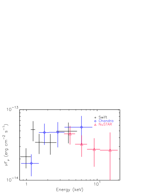
Figure 5.— X-ray SED of B21023 measured with the archival Swift, Chandra and NuSTAR data.

For B2 1023, the overall IR-to-X-ray SED we construct is very similar to that reported previously (Sbarrato et al., 2013; Ghisellini et al., 2014, 2015). However our LAT upper limits improve by over $10\times$ and this rules out the highest-$\Gamma_{\rm D}$ or the smallest-$\theta_{\rm V}$ models in Figures 2 and 3 of Sbarrato et al. (2013). Moreover our re-analysis of the NuSTAR spectrum (using $R=30^{\prime\prime}$ and $R=45^{\prime\prime}$ apertures for source and background extraction, respectively) does not agree with their finding of a steeply rising flux (Figure 5). Instead we see a break similar to that of Q0906 (Figure 2). This seems a true discrepancy in the analysis: using their reported spectral parameters WebPIMMS gives combined expected 4–20 keV count for HPD extraction from the two NuSTAR modules of 200 for their $\Gamma=1.29^{+0.14}_{-0.15}$ ($F_{\rm 5-10\,keV}=5.8\times 10^{-14}\rm\ erg\ s^{-1}\ cm^{-2}$) model and 190 counts if $\Gamma=1.60^{+0.27}_{-0.26}$ ($F_{\rm 5-10\,keV}=5.5\times 10^{-14}\rm\ erg\ s^{-1}\ cm^{-2}$). However Sbarrato et al. (2013, and we here) find only 90 detected counts. Comparing with the results for our simple power-law fit ($\Gamma=1.5\pm 0.2$ and $F_{\rm 5-10\rm\ keV}=2.5\pm 0.5\times 10^{-14}\rm\ erg\ s^{-1}\ cm^{-2}$ with cross-normalization factors of $\sim$2) we predict 90 events in good agreement with the observations. Hence a 4–20 keV extension of their rather hard inferred spectrum is difficult to accommodate. We tested additional changes to the source aperture center ($d=10^{\prime\prime}$) and size ($R=20^{\prime\prime}$), and the location of background extraction region to see if this result is sensitive to the data selection; all fits values remain consistent with those reported above and inconsistent with those of Sbarrato et al. (2013). Part of this discrepancy might be the 15% correction to the NuSTAR effective area inferred since CALDB 20131007, but this does not explain the full $2\times$ discrepancy. Possibly they renormalized the NuSTAR flux in a joint fit. If we follow the Sbarrato et al. (2013) binning to one count/bin and analyze with the cstat statistic, we find a joint fit requires a very large cross-normalization factors of $\sim$1.8–2. This might be accommodated with a large source variability, but this is not supported by the CXO and Swift data so we consider this improbable.

Over all, B2 1023 can be fit with parameters rather similar to Q0906, although we require small modifications to the disk temperature and luminosity and the synchrotron/SSC normalization (Table 2). The relatively poor X-ray S/N at the SCC peak and the lack of mid-IR detection allow a larger $\delta$ range. The Fermi bounds still limit $\delta<28$, but on the low side we can accommodate $\delta$ as small as 4. Measured $\sim 10^{12}-10^{14}$ Hz fluxes would help, lowering $\delta_{max}$, while a deeper NuSTAR exposure can pin down the typical $>10$ keV flux level to tighten up $\delta_{min}$. For example, if the soft X-ray spectrum of Sbarrato et al. (2013) really does continue, we require higher electron energies (e.g., $\gamma_{\rm e}\sim 1.5\times 10^{3}$) and can accommodate $\delta\stackrel{{\scriptstyle<}}{{{}_{\sim}}}3$ with some NuSTAR flux contributed by EC emission (see Figure 3). Note that with more limited SED coverage we did not attempt X-ray $\chi^{2}$ optimization of the model parameters as for Q0906 (Section 3.4).

The SEDs of J0131 and J1146 are even less well measured, but do show some differences from the other two. J0131 has very strong thermal disk emission and J1146 has relatively small SSC flux compared to its synchrotron emission. For the these blazars low frequency IR points are useful for estimating the synchrotron component flux, but the lack of hard X-ray measurements leaves the SCC peak frequency almost unconstrained. Thus $\gamma_{\rm e}\approx(\nu_{ssc,pk}^{obs}/\nu_{sy,pk}^{obs})^{1/2}$ is similarly unconstrained. The improved LAT upper limits from our analysis do place a bound $\delta\stackrel{{\scriptstyle<}}{{{}_{\sim}}}16$ in both cases, but $\delta$ as small as 4 seems acceptable (Figure 3 bottom). The model parameters for the $\delta=10$ case are presented in Table 2. Note that for J0131, we need a large magnetic field to prevent the EC emission from intruding on the Fermi upper limits for the given synchrotron amplitude. The model parameters we infer (Table 2) are similar to those reported in Paliya et al. (2016) for other high-$z$ blazars ($z$=2.4–4.7).

4. Discussion and Conclusions

We have analyzed new data for Q0906 taken with Gemini, NuSTAR and Fermi-LAT measurements. Our check of archival Swift exposures implies that the blazar’s X-ray emission at our new epoch is quite consistent with historical values. Indeed Q0906 has been quite constant for over 10 years and so the gamma-ray data can be averaged over the 8-yr LAT data set and combined with archival radio, IR and optical data to assemble a broad-band SED of Q0906. The Gemini spectra also provide a $\sim$4$\times 10^{9}M_{\odot}$ virial mass estimate for the BH.

In our Fermi-LAT data analysis, we do not detect Q0906, with a 95% flux upper limit in the $\sim$GeV band $\sim 10^{-13}\rm\ erg\ s^{-1}$. This is approximately two orders of magnitude lower than that implied by the EGRET excess counts. We thus infer that the excess was most likely a statistical fluctuation. Alternatively it could represent decadal-scale variability with a very bright (and soft) flare at the EGRET epoch. The NuSTAR X-ray data indicate a hard X-ray break, so that the peak of the X-ray emission, identified with the SSC component, is below 10 keV. This places a lower limit on $\delta$ so that the SSC peak matches the NuSTAR data and the EC up-scattered disk emission does not intrude on the 0.5–79 keV NuSTAR band, while the synchrotron component still explains the Spitzer flux. Thus our new measurements bound $6<\delta<11.5$ using our synchro-Compton model.

Similar and variable hard X-ray breaks have been seen in other blazars (Hayashida et al., 2015; Tagliaferri et al., 2015; Sbarrato et al., 2016; Paliya et al., 2016) and have been interpreted as an intrinsic curvature of the high-energy emission (EC or SSC; Tagliaferri et al., 2015; Hayashida et al., 2015). Our interpretation of the break is similar to that of Hayashida et al. (2015); the break is seen because the SSC peak is in the X-ray band (e.g., see Fig. 9 of Hayashida et al., 2015). Variability, although not seen in Q0906, can be explained by the variation of EC emission or $\delta$; if EC emission becomes stronger or $\delta$ lowers, the hard X-ray spectrum may become harder, extrapolating well from the low energy index.

On the observational side the $\delta$ range can be tightened if deeper NuSTAR or XMM-Newton observations refine measurement of our estimated 4 keV spectral break and $\nu_{ssc,pk}^{obs}$. Additional far-IR and sub-mm observations constrain better $\nu_{sy,pk}^{obs}$. In particular these can distinguish synchrotron emission (assumed dominant here) from thermal emission from a dust torus, as assumed for this band by e.g. Ghisellini et al. (2015). Other observations can also help. For example, Zhang et al. (2017) estimated $\delta\approx 4$ for Q0906 from radio brightness temperatures. This applies to larger radius where Compton drag should reduce $\delta$, but such measurements can at least provide an independent lower limit to $\delta$ at the jet base. On the modeling side, we note that we have assumed a jet base $h=0.03$ pc from the black hole. If this is larger the EC flux from up-scattered disk photons can be reduced since the seed photon density scales as $h^{-2}$ once $h$ exceeds the characteristic disk scale. For Q0906 this makes little difference for the allowed $\delta$ range, but it can allow larger $\delta_{max}$ for other sources where the LAT upper limits provide the effective bound.

With our new range on $\delta$ we can make inferences about the source population. The substantial $\delta_{min}=6$ means that the viewing angle $\theta_{\rm V}$ should be less than $\theta_{max}=\mathrm{cos}^{-1}(\sqrt{1-\delta_{min}^{-2}})=9.6^{\circ}$, and the chance probability to get a source seen at $\stackrel{{\scriptstyle<}}{{{}_{\sim}}}$9.6^∘ is only $\stackrel{{\scriptstyle<}}{{{}_{\sim}}}$1.4%; $\stackrel{{\scriptstyle>}}{{{}_{\sim}}}$70 similar high-mass high-$a$ BHs at a similar redshift are expected. If the true $\delta$ is larger this number increases. If we assume a distribution $\delta^{-s}$ we can compute that the fraction of all blazars seen is ($s\neq 1$)

$$f_{B}=\left[\frac{1}{2}-\frac{(1-s)}{2(\delta_{M}^{1-s}-\delta_{m}^{1-s})}\int_{\alpha_{m}}^{\alpha_{M}}{\rm sin}^{2}x{\rm cos}^{s-2}xdx\right]\times 2,$$

where $\alpha_{M}={\rm cos}^{-1}1/\delta_{M}$, $\alpha_{m}={\rm cos}^{-1}1/\delta_{m}$, and the factor 2 at the end assumes a similar jet and counter-jet. For a uniform prior ($s=0$) this is

$$f_{B}=1-\frac{1}{(\delta_{M}-\delta_{m})}\left(\alpha_{m}-\alpha_{M}+{\rm tan}\alpha_{M}-{\rm tan}\alpha_{m}\right)$$

which gives 140 unobserved blazars like Q0906 for $\delta=6-11.5$. With our weaker constraints for the other sources we obtain 230 blazars like B2 1023 and 130 each like J0131 and J1146. Of course we do not know if these four objects represent a complete sample of the $z>5$ blazar population beamed toward Earth. The targets are drawn from radio surveys so in principle areal densities of similar objects could be computed. However the completeness of the follow-up SED and spectral observations that qualify them as blazars is less certain. Also luminosity bias associated with Doppler boosting might weight the detection probability over the allowed $\delta$ range. For example Ajello et al. (2012) infer a power-law distribution with $s=2$. In this case we find

$$f_{B}=1-\frac{\delta_{M}\delta_{m}}{2(\delta_{M}-\delta_{m})}\left(\alpha_{M}-\alpha_{m}-\frac{{\rm sin}2\alpha_{M}-{\rm sin}2\alpha_{m}}{2}\right).$$

In this case we get 120 (Q0906-like), 80 (B2 1023-like) and 70 (each J0131 and J1146-like). A detailed treatment of the selection effects goes beyond the present paper, but conservatively interpreting our sample as complete, we see that the four $z>5$ objects represent a population of 620 (for uniform prior) or 350 (for $s=2$ prior) high-mass (hence luminous), high-spin (hence jet-dominated) black holes at this large redshift.

Such large numbers are interesting since from the optical SDSS survey-derived black hole mass functions in Vestergaard & Osmer (2009) we can estimate a volume density of $\sim 15{\rm Gpc^{-3}}$ $M_{\bullet}>10^{9}M_{\odot}$ active black holes in the redshift range $z=4.3\pm 0.7$. The emission detected by SDSS (optical SED and emission line detections) is nearly isotropic and the density evolution in Vestergaard & Osmer (2009)’s highest $z$ bins appears slow, so from this we estimate 3150 massive AGN in the 210 Gpc³ between $z=5$ and $z=5.5$. Thus our radio-loud blazars represent an estimated 10–20% of this population. Incompleteness of the radio blazar IDs would increase the fraction; decreased $\delta$ would lower it. But the main conclusion, that a very substantial fraction of bright high-$z$ AGN are jet dominated, seems firm.

Berti & Volonteri (2008) have studied spin distributions of BHs using numerical simulations. They focused on three cases for growth of BHs and found that depending on the growth process the final spin distribution differs. In particular, only when BHs grow with prolonged accretion there can be a significant number of high-spin black holes at $z>5$; in the cases that BHs grow via mergers or chaotic accretion only, not many BHs are expected to have large spin. Thus our SED-mediated population estimate suggests that many massive black holes had significant early disk accretion, and have been driven to high angular momentum $a$. As emphasized by Ghisellini et al. (2015), such high $a$ means high total accretion luminosity $\eta$ and, for a given Eddington flux, a lower value for the total mass accretion rate. In turn that means high BH masses at $z>5$, such as the $M_{\bullet}\approx 1.5\times 10^{10}M_{\odot}$ inferred for J0131, are very hard to achieve at such early times. Perhaps, as suggested by these authors, the very jet (which is drawing down the black hole spin energy) serves to entrain and redirect part of the accretion luminosity, allowing a larger accretion rate and faster black hole growth. Improved SED observations and modeling of these rare, but demographically important high-$z$ blazars remains the key to probing this early back hole evolution.

The Fermi LAT Collaboration acknowledges generous ongoing support from a number of agencies and institutes that have supported both the development and the operation of the LAT as well as scientific data analysis. These include the National Aeronautics and Space Administration and the Department of Energy in the United States, the Commissariat à l’Energie Atomique and the Centre National de la Recherche Scientifique / Institut National de Physique Nucléaire et de Physique des Particules in France, the Agenzia Spaziale Italiana and the Istituto Nazionale di Fisica Nucleare in Italy, the Ministry of Education, Culture, Sports, Science and Technology (MEXT), High Energy Accelerator Research Organization (KEK) and Japan Aerospace Exploration Agency (JAXA) in Japan, and the K. A. Wallenberg Foundation, the Swedish Research Council and the Swedish National Space Board in Sweden.

Additional support for science analysis during the operations phase is gratefully acknowledged from the Istituto Nazionale di Astrofisica in Italy and the Centre National d’Études Spatiales in France. This work performed in part under DOE Contract DE-AC02-76SF00515.

This work was supported in part by NASA grant NNX17AC27G under the NuSTAR guest observer program. This research was supported by Basic Science Research Program through the National Research Foundation of Korea (NRF) funded by the Ministry of Science, ICT & Future Planning (NRF-2017R1C1B2004566).

References

- Acero et al. (2015) Acero, F., Ackermann, M., Ajello, M., et al. 2015, ApJS, 218, 23
- Acero et al. (2016) —. 2016, ApJS, 223, 26
- Ackermann et al. (2015) Ackermann, M., Ajello, M., Albert, A., et al. 2015, ApJ, 799, 86
- Ackermann et al. (2017) Ackermann, M., Ajello, M., Baldini, L., et al. 2017, ApJ, 837, L5
- Ajello et al. (2012) Ajello, M., Shaw, M. S., Romani, R. W., et al. 2012, ApJ, 751, 108
- Ajello et al. (2014) Ajello, M., Romani, R. W., Gasparrini, D., et al. 2014, ApJ, 780, 73
- Atwood et al. (2013) Atwood, W., Albert, A., Baldini, L., et al. 2013, ArXiv e-prints, arXiv:1303.3514
- Atwood et al. (2009) Atwood, W. B., Abdo, A. A., Ackermann, M., et al. 2009, ApJ, 697, 1071
- Berti & Volonteri (2008) Berti, E., & Volonteri, M. 2008, ApJ, 684, 822
- Blandford & Znajek (1977) Blandford, R. D., & Znajek, R. L. 1977, MNRAS, 179, 433
- Boettcher et al. (1997) Boettcher, M., Mause, H., & Schlickeiser, R. 1997, A&A, 324, 395
- Calderone et al. (2013) Calderone, G., Ghisellini, G., Colpi, M., & Dotti, M. 2013, MNRAS, 431, 210
- Collmar et al. (2010) Collmar, W., Böttcher, M., Krichbaum, T. P., et al. 2010, A&A, 522, A66
- Fan et al. (2001) Fan, X., Narayanan, V. K., Lupton, R. H., et al. 2001, AJ, 122, 2833
- Ghisellini et al. (2014) Ghisellini, G., Sbarrato, T., Tagliaferri, G., et al. 2014, MNRAS, 440, L111
- Ghisellini et al. (2015) Ghisellini, G., Tagliaferri, G., Sbarrato, T., & Gehrels, N. 2015, MNRAS, 450, L34
- Harrison et al. (2013) Harrison, F. A., Craig, W. W., Christensen, F. E., et al. 2013, ApJ, 770, 103
- Hayashida et al. (2015) Hayashida, M., Nalewajko, K., Madejski, G. M., et al. 2015, ApJ, 807, 79
- Healey et al. (2007) Healey, S. E., Romani, R. W., Taylor, G. B., et al. 2007, ApJS, 171, 61
- Komatsu et al. (2011) Komatsu, E., Smith, K. M., Dunkley, J., et al. 2011, ApJS, 192, 18
- Madsen et al. (2015) Madsen, K. K., Harrison, F. A., Markwardt, C. B., et al. 2015, ApJS, 220, 8
- McLure & Dunlop (2004) McLure, R. J., & Dunlop, J. S. 2004, MNRAS, 352, 1390
- Mortlock et al. (2011) Mortlock, D. J., Warren, S. J., Venemans, B. P., et al. 2011, Nature, 474, 616
- Paliya et al. (2016) Paliya, V. S., Parker, M. L., Fabian, A. C., & Stalin, C. S. 2016, ApJ, 825, 74
- Romani (2006) Romani, R. W. 2006, AJ, 132, 1959
- Romani et al. (2004) Romani, R. W., Sowards-Emmerd, D., Greenhill, L., & Michelson, P. 2004, ApJ, 610, L9
- Sbarrato et al. (2013) Sbarrato, T., Tagliaferri, G., Ghisellini, G., et al. 2013, ApJ, 777, 147
- Sbarrato et al. (2016) Sbarrato, T., Ghisellini, G., Tagliaferri, G., et al. 2016, MNRAS, 462, 1542
- Shakura & Sunyaev (1973) Shakura, N. I., & Sunyaev, R. A. 1973, A&A, 24, 337
- Sowards-Emmerd et al. (2005) Sowards-Emmerd, D., Romani, R. W., Michelson, P. F., Healey, S. E., & Nolan, P. L. 2005, ApJ, 626, 95
- Tagliaferri et al. (2015) Tagliaferri, G., Ghisellini, G., Perri, M., et al. 2015, ApJ, 807, 167
- Vanden Berk et al. (2001) Vanden Berk, D. E., Richards, G. T., Bauer, A., et al. 2001, AJ, 122, 549
- Verner et al. (1996) Verner, D. A., Ferland, G. J., Korista, K. T., & Yakovlev, D. G. 1996, ApJ, 465, 487
- Vestergaard & Osmer (2009) Vestergaard, M., & Osmer, P. S. 2009, ApJ, 699, 800
- Wilms et al. (2000) Wilms, J., Allen, A., & McCray, R. 2000, ApJ, 542, 914
- Zhang et al. (2017) Zhang, Y., An, T., Frey, S., et al. 2017, MNRAS, 468, 69