Cross-Paced Representation Learning with Partial Curricula for Sketch-based Image Retrieval

Abstract

In this paper we address the problem of learning robust cross-domain representations for sketch-based image retrieval (SBIR). While most SBIR approaches focus on extracting low- and mid-level descriptors for direct feature matching, recent works have shown the benefit of learning coupled feature representations to describe data from two related sources. However, cross-domain representation learning methods are typically cast into non-convex minimization problems that are difficult to optimize, leading to unsatisfactory performance. Inspired by self-paced learning, a learning methodology designed to overcome convergence issues related to local optima by exploiting the samples in a meaningful order (i.e.  easy to hard), we introduce the cross-paced partial curriculum learning (CPPCL) framework. Compared with existing self-paced learning methods which only consider a single modality and cannot deal with prior knowledge, CPPCL is specifically designed to assess the learning pace by jointly handling data from dual sources and modality-specific prior information provided in the form of partial curricula. Additionally, thanks to the learned dictionaries, we demonstrate that the proposed CPPCL embeds robust coupled representations for SBIR. Our approach is extensively evaluated on four publicly available datasets (i.e.  CUFS, Flickr15K, QueenMary SBIR and TU-Berlin Extension datasets), showing superior performance over competing SBIR methods.

1 Introduction

In the last few years, the developments in mobile device applications have increased the demand for powerful and efficient tools to query large-scale image databases. In particular, favored by the widespread diffusion of consumer touchscreen devices, sketch-based image retrieval (SBIR) has gained popularity. Most prior works on SBIR [1, 2, 3, 4, 5] focused on designing low- and mid-level features, and used the same type of descriptors for representing both sketches and image edge maps, allowing a direct matching between the two modalities. However, these methods implicitly assume that the statistical distributions of image edges and sketches are similar. Unfortunately, this assumption does not hold in many applications. Therefore, more recent studies proposed to use different feature descriptors to better represent the different modalities and learned a shared feature space using cross-domain representation learning methods. In particular, recent approaches based on dictionary learning (DL) [6, 7, 8, 9] or deep networks [10, 11, 12, 13] have been proven especially successful for learning coupled representations from cross-modal data. However, these methods are usually based on non-convex optimization problems and can get easily stuck into local optima, with an adverse impact on the representational power and generalization capabilities of the learned descriptors.

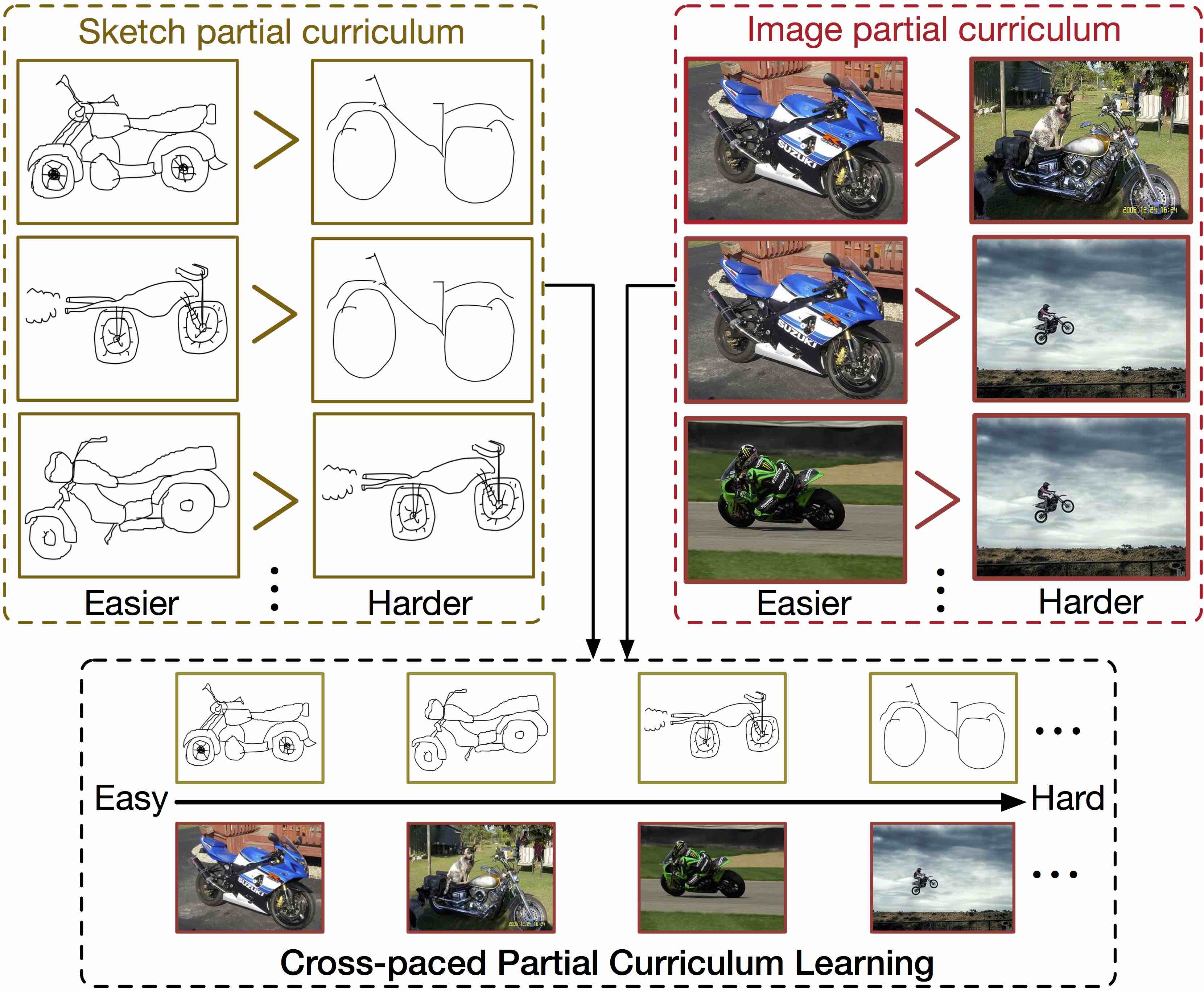
Figure 1: In real SBIR scenarios, both sketches and images show a wide range of visual complexity. Defining a-priori a full learning order (i.e. for all samples) based on the difficulty of the sketches/images is extremely challenging. Cross-paced partial curriculum learning combines the flexibility of partial modality-specific curricula with the power of self-paced learning strategies to automatically construct a full sample learning order that evolves over time until all training samples are used for learning.

Recent research efforts to overcome the problems associated to local optima resulted in two orthogonal trends: self-paced learning (SPL) [14] and curriculum learning (CL) [15]. The common denominator of both SPL and CL is to build a learning model with the help of a sample order reflecting the inherent data complexity. The rationale is that, when this order is appropriately chosen, we increase the chances of avoiding local minima. SPL and CL have been successfully applied to several computer vision tasks, such as object tracking [16] and visual category discovery [17]. Even if both strategies share a common denominator, they are quite different in spirit. Indeed, while in CL the learning order is pre-determined by an expert or according to other prior knowledge (e.g. extracted from the data), in SPL the algorithm automatically assesses the learning order usually based on the feedback of the learned model. Recently, Jiang et al.  [18] demonstrated that further advantages in terms of performance can be obtained by combining CL and SPL.

The particular case of SBIR is of special interest regarding CL, SPL and possible combinations. Indeed, as shown in Fig. 1, the visual complexity of sketches and images greatly varies, and methods attempting to exploit these variations would a priori have more chances to successfully learn efficient and robust cross-domain representations. Specifically, natural images are characterized by cluttered background and objects-of-interest captured at different scales or various poses. Similarly, sketches drawn by expert/non-expert show remarkable variations. Therefore, our aim is to turn what could be seen as an adversity, into an exploitable feature inherent to the data. However, there are two major problems which hinder the direct application of existing SPL and CL methods into cross-domain representation learning models for SBIR. Firstly, the SBIR task involves data from two different modalities, while most of the previous SPL and CL approaches are fundamentally designed to model data from a single modality. Secondly, CL methods assume the existence of a full curriculum (i.e. a complete order of all samples). This limits the applicability of CL methods to small/medium-scale problems, since the curriculum is usually designed by humans and assessing the easiness order of all samples (images and sketches) would be a chimerically resource-consuming task.

To address these problems, we design a novel cross-modality representation learning paradigm and apply it to the SBIR task. In details, we propose a novel self-paced learning strategy able to handle cross-modal data and to incorporate incomplete prior knowledge (i.e.  partial modality-specific curricula), and we name it Cross-Paced Partial Curriculum Learning (CPPCL). Furthermore, we embed this strategy into a coupled dictionary learning framework for computing robust cross-domain representations. Specifically, our method learns a pair of image- and sketch-specific dictionaries, together with the associated sparse codes, enforcing the similarity between the codes of corresponding sketches and images. The reconstruction loss with the learned dictionaries, the code correspondence and the partial modality-specific curricula jointly determine which samples to learn from. We extensively evaluate our cross-domain representation learning on four publicly available datasets (i.e.  CUFS, Flickr15K, QueenMary SBIR, TU-Berlin Extension), demonstrating the effectiveness of the proposed learning strategy and achieves superior performance over competing SBIR approaches. The main contributions of this paper are:

• We introduce the cross-paced partial curriculum learning paradigm to effectively integrate the self-pacing philosophy with modality-specific partial curricula and investigate different self-paced regularizers.

• We propose an instantiation of CPPCL within the framework of coupled dictionary learning to obtain robust cross-domain representations for SBIR and we develop an efficient algorithm to learn the modality-specific dictionaries and codes, while assessing the optimal learning order jointly from the partial curricula and the representation power of the model at the current iteration.

• We carry out an extensive experimental evaluation and analysis of the whole cross-domain representation learning framework, exhibiting its effectiveness for SBIR on four different publicly available datasets.

The paper extends our conference submission [19] by reformulating the proposed CPPCL considering different self-paced regularization terms (e.g. adding Self-paced regularizer A in Section 3.2) and developing the associated optimization algorithms (Section 4). From the experiments perspective, we discuss the influence, similarities and differences when using the different regularizing schemes within the proposed cross-paced learning framework on two publicly available datasets. A more in-depth analysis is conducted to further show the effectiveness of the proposed approach, including some parameter sensitivity study and a convergence analysis of different models (Section 5). Moreover, the introduction and related works parts are reorganized and significantly extended.

The rest of the paper is organized as follows: we first review the related work in Section 2, and then elaborate the details of the proposed approach and associated optimization algorithms in Sections 3 and 4 respectively. The experimental results are presented in Section 5 and we conclude the paper in Section 6.

2 Related Work

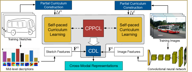
Figure 2: Overview of the proposed cross-modal representation learning method. Features extracted from sketches (e.g. LKS descriptors) and images (e.g. CNN-derived representations) are employed within a coupled dictionary learning (CDL) framework for computing cross-modal representations for SBIR. Our CDL integrates a novel cross-paced partial curriculum learning paradigm which allows the learning algorithm to start with easy samples and gradually involve hard samples according to predetermined heuristics (i.e.  modality-specific partial curricula).

This section reviews related works in the areas of: (i) sketch-based image retrieval, (ii) self-paced and curriculum learning and (iii) cross-domain dictionary learning.

2.1 Sketch-based Image Retrieval

SBIR approaches are mostly based on matching feature descriptors of the query sketch with those of the edge maps associated to the images in the database. Early works on SBIR attempted to use existing low-level feature representations (e.g.  describing color, texture, contour and shape) for both the sketch and the image modalities. Both global low-level descriptors (e.g.  color histograms [20], distribution of edge pixels [21], elastic contours [22]) and local ones (e.g.  spark descriptors [23], SYM-FISH [24], SIFT [25], HOG [26]) were investigated in the literature. Other works focused on developing specific descriptors for SBIR. For instance, Hu et al.  [1] introduced the Gradient Field HOG (GF-HOG) descriptor, extending HOG to better represent sketches, and constructed a large dataset for evaluation: the Flickr15K. Saavendra et al.  [5] also proposed a modified version of HOG, the histogram of edge local orientations (HELO), to tackle the problem of sparsity arising when HOG descriptors are applied to sketches.

To represent sketches or image edges more robustly, most recent SBIR methods focused on constructing mid- or high-level feature descriptors. Several works considered the bag-of-words (BoW) technique to aggregate low-level features and generate mid-level representations [23, 27, 28]. In addition to BoW-based methods, other approaches also focused on mid-level representations. For instance, in [4] an effective method to generate mid-level patterns, named learned keyshapes (LKS), was proposed for representing sketches. Yi et al. [29] built mid-level representations for both sketches and images by optimizing a deformable part-based model. Xiao et al. [30] designed a shape feature descriptor especially useful for preserving the shape information of sketches. A perceptual grouping framework was introduced in [31] to organize image edges into a meaningful structure and was adopted for generating human-like sketches useful for SBIR. Yu et al. [32, 33] proposed to adopt deep CNNs to learn high-level sketch representations. Similarly, Liu et al. [34] explored deep representations within a binary coding framework for fast sketch based image retrieval.

In all these works the same low- and mid/high-level representations are used to describe both the sketch and image modalities, such as to facilitate direct feature matching. However, due to the difference in appearance between sketches and images, different features are more suitable to represent the two modalities. Following this idea, some works proposed learning a shared feature space for the two modalities [35, 36]. However, none of these works considered exploiting the visual complexity of samples to learn more effective cross-modal feature representations.

2.2 Self-paced and Curriculum Learning

Inspired by the way the human brain explores the world, i.e. starting from easy concepts first and gradually involving more complex notions, self-paced learning [14] and curriculum learning [15] have been recently developed. The idea of SPL and CL is to learn models in an incremental fashion from samples with variate difficulty presented in a meaningful order. Due to their generality, these techniques have been considered in a broad spectrum of learning tasks and models, including matrix factorization [37, 18], clustering [38], multi-task learning [39] and dictionary learning [40, 36]. They have also shown to be successful in many computer vision applications such as object tracking [16], media retrieval [41], visual category discovery [17] and event detection [42].

Although self-paced learning and curriculum learning develop from the same rationale, they differ in the specific implementation schemes. In CL, the learning order (i.e.  the curriculum) is pre-defined according to prior knowledge and fixed during the learning phase, while in SPL the curriculum is dynamically determined based on the feedback from the learner. Since the sample order in SPL is dynamically inferred, one challenging task is to design a meaningful strategy of assessing the difficulty of the training samples. Previous works have addressed this issue in different ways. The most common strategy is to measure the easiness of a sample by computing the associated loss [14]. Alternatively, Jiang et al. [41] proposed to take into account the dissimilarity with respect to what has already been learned. To incorporate the benefits of both SPL and CL, a recent work [18] proposed a self-paced curriculum learning framework in which the learning order is jointly determined by a predefined full-order curriculum and the learning feedback. However, none of these previous works focused on handling multi-modal data. Our approach not only extends the self-paced learning paradigm to cope with cross-domain data, but, more importantly, is naturally able to utilize domain specific partial ordering information. In fact, opposite to the method in [18] which needs a full-order curriculum, our approach integrates prior knowledge in a form of partial curriculum. Thus, it can be applied to large scale (SBIR) tasks.

2.3 Cross-domain Dictionary Learning

Dictionary learning [6] is a popular method for finding effective sparse representations of input data. DL has been successfully applied in various image processing and computer vision tasks, such as image denoising [43] and video event detection [44]. With the fast emergence of large scale cross-domain datasets, traditional DL approaches have been extended to cross-modal tasks. For instance, Yang et al. [7] proposed to learn a set of source-specific dictionaries from samples corresponding to different domains in a coupled fashion in the context of image super-resolution. In [8] Wang et al. introduced semi-coupled DL for photo-sketch synthesis, where source-specific dictionaries are learned together with a mapping function which describes the intrinsic relationship between domains. Similarly, Huang and Wang [9] proposed a framework to simultaneously learn a pair of domain-specific dictionaries and the associated representations. Coupled DL approaches have also been applied to SBIR both in [8] and [9] and to other related tasks, such as sketch-based 3D object retrieval [45] and sketch recognition [46]. However, none of these cross-domain DL methods explore self-paced learning or curriculum learning to construct more robust features.

3 The Proposed Approach

As discussed in Section 1, in this paper we introduce a novel cross-domain representation learning framework for sketch-based image retrieval. Figure 2 shows an overview of our approach. The overall objective of the proposed model is to learn robust cross-modal feature representations. As previously mentioned, commonly used cross-modal representation leaning methods, such as coupled dictionary learning [7] and multi-modal deep learning [47], usually rely on non-convex optimization problems and are likely to get stuck at a bad local optimal. We investigate how to incorporate the ideas of SPL and partial curriculum learning within a principled unified dictionary-based learning framework.

In the following, we describe the proposed approach in details, presenting the general formulation of the overall learning problem (Section 3.1), the details of CPPCL (Section 3.2), the instantiation of CPPCL into CDL (Section 3.3) and the construction of modality-specific curricula (Section 3.4).

3.1 Problem Formulation

Let us assume the existence of $K$ sketches and denote the features extracted from the $k$-th sketch as $\mathbf{f}_{k}^{\textsc{s}}\in\mathbb{R}^{m_{\textsc{s}}}$. Similarly, we assume the existence of $L$ images and denote the features extracted from the $l$-th image as $\mathbf{f}_{l}^{\textsc{i}}\in\mathbb{R}^{m_{\textsc{i}}}$. Each sketch (resp. image) corresponds to a new cross-modal representation to be learned, denoted as $\mathbf{c}^{\textsc{s}}_{k}\in\mathbb{R}^{N}$ (resp. $\mathbf{c}^{\textsc{i}}_{l}\in\mathbb{R}^{N}$) with $N$ being the dimension of the new representation. We also define $\mathbf{F}^{\textsc{s}}=[\mathbf{f}_{1}^{\textsc{s}},\ldots,\mathbf{f}_{K}^{\textsc{s}}]\in\mathbb{R}^{m_{\textsc{s}}\times K}$ as the matrix of all sketch features, and $\mathbf{F}^{\textsc{i}}$, $\mathbf{C}^{\textsc{s}}$ and $\mathbf{C}^{\textsc{i}}$ analogously. We denote $\mathcal{U}^{\textsc{s}}$ and $\mathcal{U}^{\textsc{i}}$ as the modality-specific partial curricula constructed from the sketch and the image domains respectively. The overall learning objective of the proposed cross-paced representation learning with partial curricula model can be written as:

$$\min_{\mathbf{C}^{\textsc{s}},\mathbf{C}^{\textsc{i}},\mathbf{V}^{\textsc{j}},\bm{\xi}^{\textsc{j}}} \,\,\mathcal{L}_{\textrm{RL}}(\mathbf{C}^{\textsc{s}},\mathbf{C}^{\textsc{i}},\mathbf{V}^{\textsc{j}};\mathbf{F}^{\textsc{s}},\mathbf{F}^{\textsc{i}})$$ (1)

$$\!+\!f_{\textrm{PC}}(\bm{\xi}^{\textsc{j}};\mathcal{U}^{\textsc{s}},\mathcal{U}^{\textsc{i}})\!+\!f_{\textrm{SP}}(\mathbf{V}^{\textsc{j}};\gamma)$$

s.t. $$\,\,v_{k}^{\textsc{s}},v_{l}^{\textsc{i}}\in\{0,1\}\quad\forall k,l$$

where $\mathbf{V}^{\textsc{j}}=\textrm{diag}(\mathbf{V}^{\textsc{s}},\mathbf{V}^{\textsc{i}})$ with $\mathbf{V}^{\textsc{s}}=\textrm{diag}(v_{1}^{\textsc{s}},...,v_{K}^{\textsc{s}})$ and $\mathbf{V}^{\textsc{i}}=\textrm{diag}(v_{1}^{\textsc{i}},...,v_{L}^{\textsc{i}})$, are binary pacing variables which indicate whether a training instance (sketch or image) has to be used for learning or not. $\mathcal{L}_{\textrm{RL}}(\mathbf{C}^{\textsc{s}},\mathbf{C}^{\textsc{i}},\mathbf{V}^{\textsc{j}};\mathbf{F}^{\textsc{s}},\mathbf{F}^{\textsc{i}})$ is a cross-modal representation learning term given $\mathbf{F}^{\textsc{s}}$ and $\mathbf{F}^{\textsc{i}}$. For the proposed learning framework, this term is flexible to employ various representation learning methods such as coupled dictionary learning [9], cross-domain subspace learning [35] and deep learning [10]. $f_{\textrm{SP}}(\mathbf{V}^{\textsc{j}};\gamma)$ is a cross-modal self-paced regularizer determining the learning order of samples in two modalities, and $\gamma\geq 0$ is a self-paced parameter which controls the learning pace. $f_{\textrm{PC}}(\bm{\xi}^{\textsc{j}};\mathcal{U}^{\textsc{s}},\mathcal{U}^{\textsc{i}})$ is a partial curriculum (PC) regularizer which makes the learning order match with the pre-determined modality-specific curricula $\mathcal{U}^{\textsc{s}}$ and $\mathcal{U}^{\textsc{i}}$ as much as possible, and $\bm{\xi}^{\textsc{j}}$ represent partial curriculum learning variables. In the following, we present the details of the proposed learning framework.

3.2 Cross-paced Partial Curriculum Learning

CPPCL is a joint learning paradigm which combines a self-paced and a partial curriculum learning scheme, corresponding to the two components $f_{\textrm{PC}}(\bm{\xi}^{\textsc{j}};\mathcal{U}^{\textsc{s}},\mathcal{U}^{\textsc{i}})$ and $f_{\textrm{SP}}(\mathbf{V}^{\textsc{j}};\gamma)$ as described in Eqn. 1. By doing so, the learning order is simultaneously determined by the pre-defined prior knowledge (i.e.  partial-order modality-specific curriculum) and the feedback from the learner during training.

As mentioned in Section 3.1, in the self-paced learning philosophy, there is a pacing binary variable $v^{\textsc{s}}_{k}\in\{0,1\}$ (respectively $v^{\textsc{i}}_{l}\in\{0,1\}$) associated to sketch $k$ (respectively to image $l$), determining the learning order of the training samples. Importantly, $v^{\textsc{s}}_{k}$ and $v^{\textsc{i}}_{l}$ are not fixed and evolve during the training phase. To analyze the influence of the self-paced learning scheme, we investigate two different self-paced regularizers in our learning framework.

3.2.1 Self-paced regularizer A

is proposed to take into account the diversity of training data. We assume that the training data of the sketch modality are split into $G^{\textsc{s}}$ groups or classes (either learned from the data or provided in advance). We define a group-specific indicator vector $\mathbf{p}_{i}^{\textsc{s}}\in\mathbb{R}^{K}$, where $p_{i,k}^{\textsc{s}}=1$ if and only if sample $k$ belongs to group $i$ ($i\in\{1,...,G^{\textsc{s}}\}$), and $p_{i,k}=0$ otherwise. We devise a penalty over $\mathbf{V}^{\textsc{s}}$ that is normalized over the groups’ size, denoted by $E_{i}^{\textsc{s}}$. The definitions in the image domain, i.e. for $G^{\textsc{i}}$, $\mathbf{p}_{j}^{\textsc{i}}$ and $E_{j}^{\textsc{i}}$ are analogous. The regularizer writes:

$$f_{\textrm{SP}_{A}}(\mathbf{V}^{\textsc{j}};\gamma)=-\gamma\left(\sum_{i=1}^{G^{\textsc{s}}}\frac{1}{E_{i}^{\textsc{s}}}\|\mathbf{V}^{\textsc{s}}\mathbf{p}_{i}^{\textsc{s}}\|_{1}+\sum_{j=1}^{G^{\textsc{i}}}\frac{1}{E_{j}^{\textsc{i}}}\|\mathbf{V}^{\textsc{i}}\mathbf{p}_{j}^{\textsc{i}}\|_{1}\right).$$ (2)

This term enforces learning from different groups/classes and therefore it is closely related to SPL with diversity [42]. Similarly to [42], the idea is to learn not only from easy samples as in the standard SPL [14] but also from samples that are dissimilar from what has already been learned. However, with respect to [42], the proposed regularizer has two prominent advantages: (i) we avoid using group norms that significantly increase the complexity of the optimization solvers and (ii) we introduce the normalization factors $E_{i}^{\textsc{s}}$ and $E_{j}^{\textsc{i}}$ that soften the bias induced by dissimilar group cardinalities.

3.2.2 Self-paced regularizer B

introduces a slight modeling change. Indeed, following Zhao et al.  [37] we consider the self-pacing variables $v_{k}^{\textsc{s}}$ and $v_{l}^{\textsc{i}}$ to be continuous in the range $[0,1]$. With this choice, we allow the model to take a soft decision and assess the importance of the training sample, rather than force the method to choose between using/ignoring the sample at the current iteration. Notice that the previous self-paced regularizer ($f_{\textrm{SP}_{A}}$) can also be used with continuous self-pacing variables. In addition, considering $v_{k}^{\textsc{s}}$ and $v_{l}^{\textsc{i}}$ to be continuous opens the door to the definition of more sophisticated self-pacing regularizers such as:

$$f_{\textrm{SP}_{B}}(\mathbf{V}^{\textsc{j}};\gamma)=-\frac{\gamma}{2}\left(\sum_{k=1}^{K}Q(v_{k}^{\textsc{s}})+\sum_{l=1}^{L}Q(v_{l}^{\textsc{i}})\right),$$ (3)

where $Q(v)=v^{2}-2v$ as in [37].

Importantly, the penalty induced by the regularizer evolves over time so as to incorporate more and more samples to be part of the training set. Specifically, the self-paced parameter $\gamma$ is multiplied by a step size $\eta$ ($\eta>1$) in order to increase $\gamma$ at each iteration, as in traditional SPL methods [14]. This is done for both $f_{\textrm{SP}_{A}}$ and $f_{\textrm{SP}_{B}}$ regularizers.

An important methodological contribution of our work is to include modality-specific partial curricula into a representation learning framework and to study its behavior within the SPL strategy already discussed. Subsequently, we assume the existence of two modality-specific sets of constraints ${\cal U}^{\textsc{s}}$ and ${\cal U}^{\textsc{i}}$. Each element of the sets consists of an index pair representing that if $(k,k^{\prime})\in{\cal U}^{\textsc{s}}$, then $v^{\textsc{s}}_{k}<v^{\textsc{s}}_{k^{\prime}}$ and learning should be performed considering a priori $\mathbf{f}^{\textsc{s}}_{k^{\prime}}$ before $\mathbf{f}^{\textsc{s}}_{k}$, as it corresponds to an easier sample. Depending on the way the curricula are constructed ${\cal U}^{\textsc{s}}$ could contain incompatibilities, for instance, $\{(k,k^{\prime}),(k^{\prime},k^{\prime\prime}),(k^{\prime\prime},k)\}\subset{\cal U}^{\textsc{s}}$. In addition, the cross-modal terms could also induce incompatibilities between the two modalities. Therefore, it is desirable to relax the constraints using a set of slack variables $\xi_{kk^{\prime}}^{\textsc{s}}$, $\xi_{ll^{\prime}}^{\textsc{i}}$, and the partial curriculum regularizer is written as:

$$f_{\textrm{PC}}(\bm{\xi}^{\textsc{j}};\mathcal{U}^{\textsc{s}},\mathcal{U}^{\textsc{i}})=\mu\left(\sum_{(k,k^{\prime})\in{\cal U}^{\textsc{s}}}\xi_{kk^{\prime}}^{\textsc{s}}+\sum_{(l,l^{\prime})\in{\cal U}^{\textsc{i}}}\xi_{ll^{\prime}}^{\textsc{i}}\right),$$ (4)

where $\bm{\xi}^{\textsc{j}}=[[\xi_{kk^{\prime}}^{\textsc{s}}]_{(k,k^{\prime})\in{\cal U}^{\textsc{s}}}[\xi_{ll^{\prime}}^{\textsc{i}}]_{(l,l^{\prime})\in{\cal U}^{\textsc{i}}}]$ is the vector of all slack variables and $f_{\textrm{PC}}$ is the partial curricula regularizer regulated by the parameter $\mu\geq 0$. In all, the optimization problem of CPPCL writes:

$$\min_{\mathbf{V}^{\textsc{j}},\bm{\xi}^{\textsc{j}}} \,\,f_{\textrm{PC}}(\bm{\xi}^{\textsc{j}};\mathcal{U}^{\textsc{s}},\mathcal{U}^{\textsc{i}})+f_{\textrm{SP}}(\mathbf{V}^{\textsc{j}};\gamma)$$

$$\,\,v_{k}^{\textsc{s}},v_{l}^{\textsc{i}}\in\{0,1\}\quad\forall k,l,$$

$$\,\,v_{k}^{\textsc{s}}-v_{k^{\prime}}^{\textsc{s}}<\xi_{kk^{\prime}}^{\textsc{s}},\,\xi_{kk^{\prime}}^{\textsc{s}}\geq 0,\,\forall(k,k^{\prime})\in{\cal U}^{\textsc{s}}$$

$$\,\,v_{l}^{\textsc{i}}-v_{l^{\prime}}^{\textsc{i}}<\xi_{ll^{\prime}}^{\textsc{i}},\,\xi_{ll^{\prime}}^{\textsc{i}}\geq 0,\,\forall(l,l^{\prime})\in{\cal U}^{\textsc{i}}.$$

3.3 Instantiation of CPPCL into CDL

To learn cross-modal representations for SBIR, we embed the CPPCL into a coupled dictionary learning framework. Given the feature matrices $\mathbf{F}^{\textsc{s}}$ and $\mathbf{F}^{\textsc{i}}$ of the sketch and image domain, and two $N$-word dictionaries, one per modality: $\mathbf{D}^{\textsc{s}}=[\mathbf{d}_{n}^{\textsc{s}}]_{n=1}^{N}\in\mathbb{R}^{m_{\textsc{s}}\times N}$ and $\mathbf{D}^{\textsc{i}}=[\mathbf{d}_{n}^{\textsc{i}}]_{n=1}^{N}\in\mathbb{R}^{m_{\textsc{i}}\times N}$, we learn the associated dictionaries $\mathbf{D}^{\textsc{s}}$, $\mathbf{D}^{\textsc{i}}$ and sparse representations $\mathbf{C}^{\textsc{s}},\mathbf{C}^{\textsc{i}}$ by minimizing the following objective function:

$$\mathcal{L}_{\textrm{RL}}=\|(\mathbf{F}^{\textsc{s}}-\mathbf{D}^{\textsc{s}}\mathbf{C}^{\textsc{s}})\mathbf{V}^{\textsc{s}}\|^{2}_{\mathcal{F}}+\|(\mathbf{F}^{\textsc{i}}-\mathbf{D}^{\textsc{i}}\mathbf{C}^{\textsc{i}})\mathbf{V}^{\textsc{i}}\|^{2}_{\mathcal{F}}$$

$$+\alpha\left(\|\mathbf{C}^{\textsc{s}}\|_{1}+\|\mathbf{C}^{\textsc{i}}\|_{1}\right)+\beta\,\textrm{Tr}\left(\mathbf{C}^{\textsc{j}}\mathbf{V}^{\textsc{j}}\mathbf{L}\mathbf{V}^{\textsc{j}\top}\mathbf{C}^{\textsc{j}\top}\right),$$

subject to:

$$\|\mathbf{d}_{n}^{\textsc{s}}\|,\|\mathbf{d}_{n}^{\textsc{i}}\|\leq 1\quad\forall n,\qquad v_{k}^{\textsc{s}},v_{l}^{\textsc{i}}\in\{0,1\}\quad\forall k,l,$$

where $\alpha\geq 0$ is a regularization parameter and $\|\cdot\|_{\mathcal{F}}$ denotes the Frobenius norm. The constraints remove any scale ambiguities due to the matrix products $\mathbf{D}^{\textsc{s}}\mathbf{C}^{\textsc{s}}$ and $\mathbf{D}^{\textsc{i}}\mathbf{C}^{\textsc{i}}$, while the regularization terms induce sparsity in the learned codes.

We also introduce a graph Laplacian regularizer to maintain the relational link between the learned representations of sketches and images in the training set. Ideally, each sketch corresponds to at least an image (e.g. for sketch to photo face recognition [48] in the context of security and biometrics applications). Alternatively, the association among sketches and images is derived from image class information [1]. Generally speaking, in this paper we consider both intra-modality and cross-modality relationships, modeled by a non-negative weight matrix $\mathbf{W}\in\mathbb{R}^{+\,(K+L)\times(K+L)}$. Intuitively, the larger $w_{pq}$ is, the stronger the relationship between the $p$-th and $q$-th codes is. Importantly, when $1\leq p,q\leq K$ (respectively, $K<p,q\leq K+L$), $w_{pq}$ relates two sketches (respectively, two images) creating an intra-modality link, otherwise $w_{pq}$ relates a sketch and an image (cross-modality link). Interpreting $\mathbf{W}$ as the weight matrix of a graph and denoting the associated Laplacian matrix by $\mathbf{L}$, a graph laplacian regularizer for the codes is defined as $\textrm{Tr}\left(\mathbf{C}^{\textsc{j}}\mathbf{L}\mathbf{C}^{\textsc{j}\top}\right)=\frac{1}{2}\sum_{p,q=1}^{K+L}w_{pq}\|\mathbf{c}^{\textsc{j}}_{p}-\mathbf{c}^{\textsc{j}}_{q}\|^{2}$, where $\mathbf{C}^{\textsc{j}}=[\mathbf{c}^{\textsc{j}}_{p}]_{p=1}^{K+L}=[\mathbf{C}^{\textsc{s}}\,\mathbf{C}^{\textsc{i}}]\in\mathbb{R}^{N\times(K+L)}$ is a joint code matrix, and $\beta\geq 0$ is a regularization parameter controlling the importance of the relational knowledge. By embedding pacing variables $\mathbf{V}^{\textsc{j}}$ into $\textrm{Tr}\left(\mathbf{C}^{\textsc{j}}\mathbf{L}\mathbf{C}^{\textsc{j}\top}\right)$, we obtain the self-paced graph laplacian regularizer $\textrm{Tr}\left(\mathbf{C}^{\textsc{j}}\mathbf{V}^{\textsc{j}}\mathbf{L}\mathbf{V}^{\textsc{j}\top}\mathbf{C}^{\textsc{j}\top}\right)$. Finally, the optimization problem to solve for writes:

$$\min_{\mathbf{D}^{\textsc{s}},\mathbf{D}^{\textsc{i}},\mathbf{C}^{\textsc{j}},\mathbf{V}^{\textsc{j}},\mathbf{\xi}^{\textsc{j}}} \,\,\mathcal{L}_{\textrm{RL}}\!+\!f_{\textrm{PC}}(\bm{\xi}^{\textsc{j}};\mathcal{U}^{\textsc{s}},\mathcal{U}^{\textsc{i}})\!+\!f_{\textrm{SP}}(\mathbf{V}^{\textsc{j}},\gamma)$$ (5)

s.t. $$\,\,\|\mathbf{d}_{n}^{\textsc{s}}\|,\|\mathbf{d}_{n}^{\textsc{i}}\|\leq 1\quad\forall n,$$

$$\,\,v_{k}^{\textsc{s}},v_{l}^{\textsc{i}}\in\{0,1\}\quad\forall k,l,$$

$$\,\,v_{k}^{\textsc{s}}-v_{k^{\prime}}^{\textsc{s}}<\xi_{kk^{\prime}}^{\textsc{s}},\,\xi_{kk^{\prime}}^{\textsc{s}}\geq 0,\,\forall(k,k^{\prime})\in{\cal U}^{\textsc{s}}$$

$$\,\,v_{l}^{\textsc{i}}-v_{l^{\prime}}^{\textsc{i}}<\xi_{ll^{\prime}}^{\textsc{i}},\,\xi_{ll^{\prime}}^{\textsc{i}}\geq 0,\,\forall(l,l^{\prime})\in{\cal U}^{\textsc{i}}.$$

3.4 Laplacian and Curricula Construction

In this section we describe how we construct the modality-specific partial curricula and the Laplacian matrix representing the relational knowledge. However, it is worth noting that our approach is general and other design choices are possible. We build both the curricula and the Laplacian in the training set from the sketch and image features and a group association, that could arise from the class membership or from unsupervised clustering. In our experiments, we also devised a protocol to construct a curriculum for sketches from human manual annotations.

3.4.1 Construction of graph Laplacian matrix

To build the Laplacian matrix (computed from the weights $w_{pq}$), the intra-modality relationships are defined using the Gaussian kernel and the inter-modality with group association, as in [49]:

$${w_{pq}}=\left\{\begin{array}[]{l}\textrm{e}^{-\left\|\mathbf{f}_{p}^{\textsc{s}}-\mathbf{f}_{q}^{\textsc{s}}\right\|_{2}^{2}/2{\sigma^{2}}},\quad p,q\leq K\\ \textrm{e}^{-\left\|\mathbf{f}_{p-K}^{\textsc{i}}-\mathbf{f}_{q-K}^{\textsc{i}}\right\|_{2}^{2}/2{\sigma^{2}}},\quad K<p,q\\ 1,\quad\begin{array}[]{l}p\leq K<q\text{ and $p\sim q$}\\ q\leq K<p\text{ and $q\sim p$}\end{array}\\ 0,\quad\text{otherwise,}\end{array}\right.$$ (6)

where $\sigma$ is the Gaussian kernel parameter fixed to $1$ with no significant performance variation around this value. The symbol $\sim$ indicates samples belonging to the same cluster/class.

3.4.2 Construction of modality-specific curricula

Regarding the curricula construction, as stated above, a fundamental aspect of the the proposed framework is the possibility to handle partial curricula. Previous CL or hybrid CL-SPL methods [15, 18] instead assume that a full curriculum, i.e. a complete order of samples, is provided. This is a strong assumption that may be unrealistic in real-world large-scale tasks. On the one hand, even if automatic measures of the easiness of an image [17] have been developed, these metrics are accurate up to some extent and therefore deriving a full ranking from these measures may be inappropriate. On the other hand, manually annotating the entire set of images represents a huge human workload, highly demanding for medium and large-scale datasets. In addition, if the multi-modal dataset is gathered incrementally, the cost of updating the curriculum grows with the size of the dataset.

Image partial curricula

The partial curricula for the image domain is obtained by means of an automated procedure based on previous studies [17, 50]. Intuitively, easy images are those containing non-occluded high-resolution objects in low-cluttered background. Previous works [17] proposed to define the easiness of an image from the “objectness” measures [50]. In the same line of though, we compute the easiness measure as the median of the 30 highest “objectness” scores among a set of 1,000 window proposals. An example is shown in Figure 3. This procedure approximates the easiness of a training image. Notice that, two images with largely different scores are likely to correspond to samples with different easiness. On the contrary, if the scores are similar, imposing that the image with the lowest score is the easiest in the pair may induce some errors. The constraint associated to an image pair is included in ${\cal U}^{\textsc{i}}$ only if the difference of their associated scores exceeds a certain threshold $\delta^{\textsc{i}}$ (i.e.  if one of the images in the pair is significantly easier than the other).

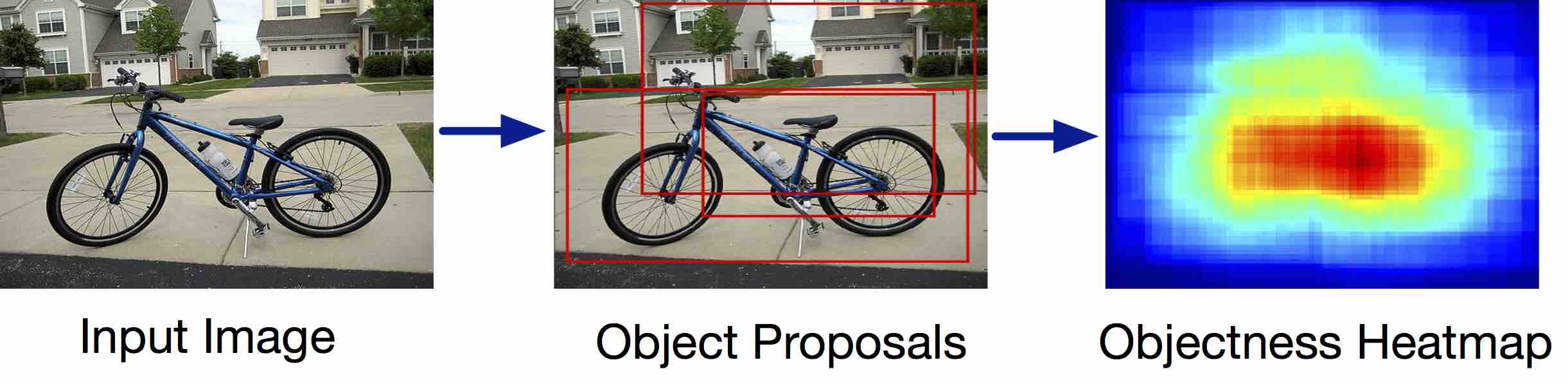
Figure 3: An illustration of objectness generation process for assessing the easiness of an image sample.

Figure 4: The graphical interface used for annotation. Easy sketches are those with more details and easy images are those with non-occluded high-resolution objects in low-cluttered background.

Sketch partial curricula

Contrary to the image domain, there is no widely-accepted procedure to define the easiness of a sketch. Therefore, we consider two methods for constructing the partial curriculum in the sketch domain. The first one is an automatic method that follows again the philosophy of [50]. Given a sketch, we randomly sample 100 windows at different scales and positions. For each window we compute the “edgeness” score, representing the edge density within the window as proposed in [50]. Intuitively, the edgeness should follow the rationale that easy sketches are those with more details. As previously done for images, the constraint associated to a pair of sketches is included into ${\cal U}^{\textsc{s}}$ only if their measure of edgeness differs by at least $\delta^{\textsc{s}}$. The second one is a semi-automatic strategy for building the partial curricula of the sketches by including human annotators in the loop. A naive retrieval method based on SHOG features [23] generates potential constraints (pairs of sketches). In details, we pair each sketch with the closest among the cluster/class. The human annotator is then queried which sketch is easier to learn from. Ten PhD students (6 male, 4 female) of age $24.3\pm 1.4$ (mean, standard deviation) performed the annotation after being instructed that “easy” sketches meant sketches with more details. Importantly, since CPPCL is specifically designed to handle partial curricula, annotators had the possibility to “skip” sketch pairs if they were unable to decide. A simple GUI, shown in Figure 4, was developed for annotation.

4 Model Optimization

The optimization problem in Eqn. 5 is not jointly convex in all variables. However, efficient alternate optimization techniques can solve it since it is convex on $\{\mathbf{D}^{\textsc{s}},\mathbf{D}^{\textsc{i}}\}$, $\{\mathbf{C}^{\textsc{j}}\}$ and $\{\mathbf{V}^{\textsc{j}},\bm{\xi}^{\textsc{j}}\}$ when the other two sets of variables are fixed. We proposed two different self-paced regularizers $f_{\textrm{SP}_{A}}$ and $f_{\textrm{SP}_{B}}$ in our model. However, they have no impact when solving for $\mathbf{D}^{\textsc{s}}$ and $\mathbf{D}^{\textsc{i}}$, while we provide two different solutions for solving $\mathbf{V}^{\textsc{j}}$ and $\bm{\xi}^{\textsc{j}}$.

4.0.1 Solve for $\mathbf{D}^{\textsc{s}}$ and $\mathbf{D}^{\textsc{i}}$

Fixing $\mathbf{C}^{\textsc{j}}$, $\mathbf{V}^{\textsc{j}}$ and $\bm{\xi}^{\textsc{j}}$, the optimization problem for $\mathbf{D}^{\textsc{s}}$ (analogously for $\mathbf{D}^{\textsc{i}}$) writes:

$$\mathop{\min}\limits_{{\mathbf{D}^{\textsc{s}}}}{\left\|{({\mathbf{F}^{\textsc{s}}}-{\mathbf{D}^{\textsc{s}}}{\mathbf{C}^{\textsc{s}}})\mathbf{V}^{\textsc{s}}}\right\|_{2}^{2}}\quad\textrm{s.t. }\left\|{{\mathbf{d}^{\textsc{s}}_{k}}}\right\|\leq 1.$$ (7)

This problem is a Quadratically Constrained Quadratic Program (QCQP) that can be solved using gradient descent with e.g. Lagrangian duality [6].

4.0.2 Solve for $\mathbf{C}^{\textsc{j}}$

By fixing $\mathbf{D}^{\textsc{s}}$, $\mathbf{D}^{\textsc{i}}$, $\mathbf{V}^{\textsc{j}}$ and $\bm{\xi}^{\textsc{j}}$ the optimization function for the codes can be rewritten as:

$$f(\mathbf{C}^{\textsc{j}}) =\left\|\left(\mathbf{F}^{\textsc{s}}-\mathbf{D}^{\textsc{s}}\mathbf{C}^{\textsc{s}}\right)\mathbf{V}^{\textsc{s}}\right\|_{\cal F}^{2}+\left\|\left(\mathbf{F}^{\textsc{i}}-\mathbf{D}^{\textsc{i}}\mathbf{C}^{\textsc{i}}\right)\mathbf{V}^{\textsc{i}}\right\|_{\cal F}^{2}$$

$$+\alpha\left\|\mathbf{C}^{\textsc{j}}\right\|_{1}+\beta\,\textrm{Tr}\left(\mathbf{C}^{\textsc{j}}\mathbf{V}^{\textsc{j}}\mathbf{L}\mathbf{V}^{\textsc{j}\top}\mathbf{C}^{\textsc{j}\top}\right).$$ (8)

According to FISTA [51], $f$ can be viewed as a proximal regularization problem, solved using the following recursion (over $r$):

$$\mathbf{C}^{\textsc{j}}_{r}\!=\!\mathop{\arg\!\min}\limits_{{\mathbf{C}^{\textsc{j}}}}\!\left\{\frac{\left\|{{\mathbf{C}^{\textsc{j}}}\!-\!\mathbf{C}^{\textsc{j}}_{r-1}\!+\!{t_{r}}\nabla\!f\!(\mathbf{C}^{\textsc{j}}_{r-1})}\right\|_{\cal F}^{2}}{2t_{r}}+{\alpha}{\left\|{{\mathbf{C}^{\textsc{j}}}}\right\|_{1}}\right\},$$ (9)

where $t_{r}>0$ is the step size and $\nabla\!f(\mathbf{C}^{\textsc{j}})=[\nabla\!f(\mathbf{C}^{\textsc{s}})\;\nabla\!f(\mathbf{C}^{\textsc{i}})]$ is the concatenation of the two gradients defined as:

$$\nabla\!f(\mathbf{C}^{\textsc{s}}) =2\mathbf{D}^{\textsc{s}\top}(\mathbf{D}^{\textsc{s}}\mathbf{C}^{\textsc{s}}-\mathbf{F}^{\textsc{s}})(\mathbf{V}^{\textsc{s}})^{2}$$

$$+2\beta\left(\mathbf{C}^{\textsc{s}}\mathbf{V}^{\textsc{s}}\mathbf{L}^{\textsc{s}}+\mathbf{C}^{\textsc{i}}\mathbf{V}^{\textsc{i}}\mathbf{L}^{\textsc{i}\textsc{s}}\right)\mathbf{V}^{\textsc{s}},$$ (10)

where the sublaplacian matrices are taken from the Laplacian matrix as $\mathbf{L}=[\mathbf{L}^{\textsc{s}}\,\mathbf{L}^{\textsc{s}\textsc{i}};\mathbf{L}^{\textsc{i}\textsc{s}}\,\mathbf{L}^{\textsc{i}}]$. The second gradient, $\nabla\!f(\mathbf{C}^{\textsc{i}})$ is defined analogously to $\nabla\!f(\mathbf{C}^{\textsc{s}})$. Moreover, (9) is a standard LASSO problem whose optimal solution can be found using the feature-sign search algorithm in [6].

4.0.3 Solve for $\mathbf{V}^{\textsc{j}}$ and $\bm{\xi}^{\textsc{j}}$ with the regularizer $f_{\textrm{SP}_{A}}$

We fix $\mathbf{D}^{\textsc{s}}$, $\mathbf{D}^{\textsc{i}}$, $\mathbf{C}^{\textsc{j}}$ to solve for $\bm{\xi}^{\textsc{j}}$ and $\mathbf{V}^{\textsc{j}}$, and the problem writes:

$$\min_{\mathbf{V}^{\textsc{j}}} \mathcal{L}_{\textrm{RL}}-\gamma\left(\sum_{k=1}^{K}\frac{1}{E_{g,k}^{\textsc{s}}}v_{k}^{\textsc{s}}+\sum_{l=1}^{L}\frac{1}{E_{g^{\prime},l}^{\textsc{i}}}v_{l}^{\textsc{i}}\right),$$ (11)

$$+\mu\left(\sum_{(k,k^{\prime})\in{\cal U}^{\textsc{s}}}\xi_{kk^{\prime}}^{\textsc{s}}+\sum_{(l,l^{\prime})\in{\cal U}^{\textsc{i}}}\xi_{ll^{\prime}}^{\textsc{i}}\right)$$

s.t. $$0\leq v_{k}^{\textsc{s}},v_{l}^{\textsc{i}}\leq 1\quad\forall k,l,$$

$$v_{k}^{\textsc{s}}-v_{k^{\prime}}^{\textsc{s}}<\xi_{kk^{\prime}}^{\textsc{s}},\,\xi_{kk^{\prime}}^{\textsc{s}}\geq 0,\,\forall(k,k^{\prime})\in{\cal U}^{\textsc{s}},$$

$$v_{l}^{\textsc{i}}-v_{l^{\prime}}^{\textsc{i}}<\xi_{ll^{\prime}}^{\textsc{i}},\,\xi_{ll^{\prime}}^{\textsc{i}}\geq 0,\,\forall(l,l^{\prime})\in{\cal U}^{\textsc{i}}.$$

Here we replace the self-paced regularizer $\sum_{g=1}^{G^{\textsc{s}}}\frac{1}{E_{g}^{\textsc{s}}}\|\mathbf{V}^{\textsc{s}}\mathbf{p}_{g}^{\textsc{s}}\|_{1}$ with $\sum_{k=1}^{K}\sum_{g=1}^{G^{\textsc{s}}}\frac{1}{E_{g}^{\textsc{s}}}p_{g,k}^{\textsc{s}}v_{k}^{\textsc{s}}=\sum_{k=1}^{K}\frac{1}{E_{g,k}^{\textsc{s}}}v_{k}^{\textsc{s}}$ since $v_{i}\geq 0$, $E_{g,k}^{\textsc{s}}$ being the size of group/class $g$ of sample $k$. As discussed in Section 3.2 and following [37, 38], the self-paced regularizer can be used with continuous self-pacing variables for facilitating the optimization. This property is particularly advantageous in our case, because the joint $(\mathbf{V}^{\textsc{j}},\bm{\xi}^{\textsc{j}})$ optimization problem can now be treated as a quadratic programming (QP) problem with a set of linear inequality constraints. Recent studies have shown that this strategy, as opposed to solving the original mixed integer quadratic programming problem, is successful in several applications [37, 18].

Let $\mathbf{y}=[[v_{k}^{\textsc{s}}]_{k}[v_{l}^{\textsc{i}}]_{l}[\xi^{\textsc{s}}_{kk^{\prime}}]_{kk^{\prime}}[\xi^{\textsc{i}}_{ll^{\prime}}]_{ll^{\prime}}]\in\mathbb{R}^{K+L+C^{\textsc{s}}+C^{\textsc{i}}}$ denote the joint optimization variable for which the problem writes:

$$\min_{\mathbf{y}} \,\,\mathbf{y}^{\top}\mathbf{R}\mathbf{y}+\mathbf{b}^{\top}\mathbf{y}$$ (12)

s.t. $$\,\,\mathbf{G}\mathbf{y}\leq\mathbf{h},$$

where the values of $\mathbf{R}$, $\mathbf{b}$, $\mathbf{G}$ and $\mathbf{h}$ are defined in the following. $\mathbf{R}$ is a $(K+L+C^{\textsc{s}}+C^{\textsc{i}})\times(K+L+C^{\textsc{s}}+C^{\textsc{i}})$ matrix with all zeros except for the first $(K+L)\times(K+L)$ block, where $C^{\textsc{s}}$ and $C^{\textsc{i}}$ denote the number of constraints of the sketch and the image modality respectively. More precisely:

$$R_{pq}=\left\{\begin{array}[]{ll}\|\mathbf{f}_{p}^{\textsc{s}}-\mathbf{D}^{\textsc{s}}\mathbf{c}_{p}^{\textsc{s}}\|^{2}&q=p\leq K\\ \|\mathbf{f}_{p-K}^{\textsc{i}}-\mathbf{D}^{\textsc{i}}\mathbf{c}_{p-K}^{\textsc{i}}\|^{2}&K<q=p\leq L+K\\ \beta w_{pq}\|\mathbf{c}_{p}^{\textsc{j}}-\mathbf{c}_{q}^{\textsc{j}}\|^{2}&1\leq p\neq q\leq K+L\\ 0&\text{otherwise}\end{array}\right.$$

and $\mathbf{b}=[-\frac{\gamma}{E_{g,1}^{\textsc{s}}},...,-\frac{\gamma}{E_{g,K}^{\textsc{s}}},-\frac{\gamma}{E_{g^{\prime},1}^{\textsc{i}}},...,-\frac{\gamma}{E_{g^{\prime},L}^{\textsc{i}}},\,\,\mu\mathbf{1}_{C^{\textsc{s}}+C^{\textsc{i}}}^{\top}]^{\top}$, where $\mathbf{1}_{C}$ is a $C\times 1$ vector filled with ones. $\mathbf{G}$ and $\mathbf{h}$ represent the inequality and bound constraints in (5) and their derivation is straightforward. Since there are $2(K+L+C^{\textsc{s}}+C^{\textsc{i}})$ constraints, $\mathbf{G}\in\mathbb{R}^{2(K+L+C^{\textsc{s}}+C^{\textsc{i}})\times(K+L+C^{\textsc{s}}+C^{\textsc{i}})}$ and $\mathbf{h}\in\mathbb{R}^{2(K+L)+C^{\textsc{s}}+C^{\textsc{i}}}$.

4.0.4 Solve for $\mathbf{V}^{\textsc{j}}$ and $\bm{\xi}^{\textsc{j}}$ with the regularizer $f_{\textrm{SP}_{B}}$

Similar to the previous case with the regularizer $f_{\textrm{SP}_{A}}$, by fixing the dictionaries $\mathbf{D}^{\textsc{s}}$, $\mathbf{D}^{\textsc{i}}$ and the codes $\mathbf{C}^{\textsc{j}}$, the optimization problem is also a QP problem, and the only difference is that $R_{pq}$ and $\mathbf{b}$ change. In this case, $\mathbf{b}=[\gamma\mathbf{1}_{K+L}^{\top}\,\,\mu\mathbf{1}_{C^{\textsc{s}}+C^{\textsc{i}}}^{\top}]^{\top}$ and $R_{pq}$ becomes:

$$R_{pq}=\left\{\begin{array}[]{ll}\|\mathbf{f}_{p}^{\textsc{s}}-\mathbf{D}^{\textsc{s}}\mathbf{c}_{p}^{\textsc{s}}\|^{2}-\gamma/2&q=p\leq K\\ \|\mathbf{f}_{p-K}^{\textsc{i}}-\mathbf{D}^{\textsc{i}}\mathbf{c}_{p-K}^{\textsc{i}}\|^{2}-\gamma/2&K<q=p\leq L+K\\ \beta w_{pq}\|\mathbf{c}_{p}^{\textsc{j}}-\mathbf{c}_{q}^{\textsc{j}}\|^{2}&1\leq p\neq q\leq K+L\\ 0&\text{otherwise}\end{array}\right.$$

Then the QP problem can be effectively solved with the interior-point algorithms [52]. The full optimization procedure is shown in Algorithm 1.

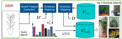
Figure 5: An illustration of the test phase of the proposed model for SBIR.

Input: the features $\mathbf{F}^{\textsc{s}}$, $\mathbf{F}^{\textsc{i}}$ and the parameters $\alpha$, $\beta$, $\gamma$, $\mu$

Output: $\mathbf{D}^{\textsc{s}}$, $\mathbf{C}^{\textsc{s}}$, $\mathbf{D}^{\textsc{i}}$, $\mathbf{C}^{\textsc{i}}$

1 Initialize $\mathbf{D}^{\textsc{s}}$, $\mathbf{C}^{\textsc{s}}$, $\mathbf{D}^{\textsc{i}}$, $\mathbf{C}^{\textsc{i}}$ as described in Section 5 and initialize a step size $\eta$ ($\eta>1$);

2 while not converged do

3       Update $\mathbf{V}^{\textsc{j}}$ and $\bm{\xi}^{\textsc{j}}$ following (12);

4       Update $\mathbf{C}^{\textsc{s}}$, $\mathbf{C}^{\textsc{i}}$ with (9);

5       Update $\mathbf{D}^{\textsc{s}}$, $\mathbf{D}^{\textsc{i}}$ by solving (7);

6       $\gamma\leftarrow\eta\gamma$;

7 end while

return $\mathbf{D}^{\textsc{s}^{\star}}$, $\mathbf{C}^{\textsc{s}^{\star}}$, $\mathbf{D}^{\textsc{i}^{\star}}$, $\mathbf{C}^{\textsc{i}^{\star}}$

Algorithm 1 Optimization Procedure

4.0.5 Test Phase for Sketch-to-Image Retrieval

Fig. 5 depicts the test phase of the proposed approach. Given the learned dictionaries $\mathbf{D}^{\textsc{i}}$ and features of the retrieval images $\mathbf{F}^{\textsc{i}}_{\textsc{TEST}}$, we perform a dictionary mapping to calculate all the sparse representations $\mathbf{C}^{\textsc{i}}_{\textsc{TEST}}$ of the retrieval sketches via solving:

$$\mathop{\min}\limits_{{\mathbf{C}^{\textsc{i}}_{\textsc{TEST}}}}{\left\|{({\mathbf{F}^{\textsc{i}}_{\textsc{TEST}}}-{\mathbf{D}^{\textsc{i}}}{\mathbf{C}^{\textsc{i}}_{\textsc{TEST}}})}\right\|_{\cal{F}}^{2}}+\alpha\left\|{{\mathbf{C}^{\textsc{i}}_{\textsc{TEST}}}}\right\|_{1}.$$ (13)

For a query sketch $k$, a corresponding sparse representation $\mathbf{c}_{k}^{\textsc{s}}$ can be calculated by a similar dictionary mapping with $\mathbf{D}^{\textsc{s}}$ as in Eqn. (13). Then we retrieve top $K$ results from $\mathbf{C}^{\textsc{i}}_{\textsc{TEST}}$ using $K$ Nearest Neighbor ($K$-NN), while for tests on sketch-to-face recognition, a Nearest Neighbor classifier is used.

5 Experiments

To evaluate the effectiveness of our approach for Cross-Paced Representation Learning (CPRL), we conduct extensive experiments on four publicly available datasets: the CUHK Face Sketch (CUFS) [48], the Flickr15k [1], the Queen Mary SBIR [29] and the TU-Berlin Extension [53] datasets.

5.1 Implementation Details

The experiments were run on a PC with a quad core (2.1 GHz) CPU, 64GB RAM and an Nvidia Tesla K40 GPU. The proposed SBIR approach is implemented in Matlab and partially in C++ (the most computationally expensive components). For representing sketches, we adopted the mid-level representation method named Learned KeyShapes (LKS) [4]. We used a C++ implementation for efficient extraction of LKS features and wrap it in a Matlab interface. For representing images, CNN features were used. Specifically, the Caffe reference network ‘AlexNet’ pre-trained on ImageNet was used to extract features from the sixth (the first fully connected) layer. In all our experiments and for all datasets, the value of the self-paced parameter was initialized to $\gamma=1$ and increased by a factor $\eta=1.3$ at each iteration (until all the training samples are selected). The dictionaries $\mathbf{D}^{\textsc{s}}$ and $\mathbf{D}^{\textsc{i}}$ were initialized with joint DL [7] when both features have the same dimension and with modality-independent DL otherwise.

5.2 Sketch-to-Face Recognition

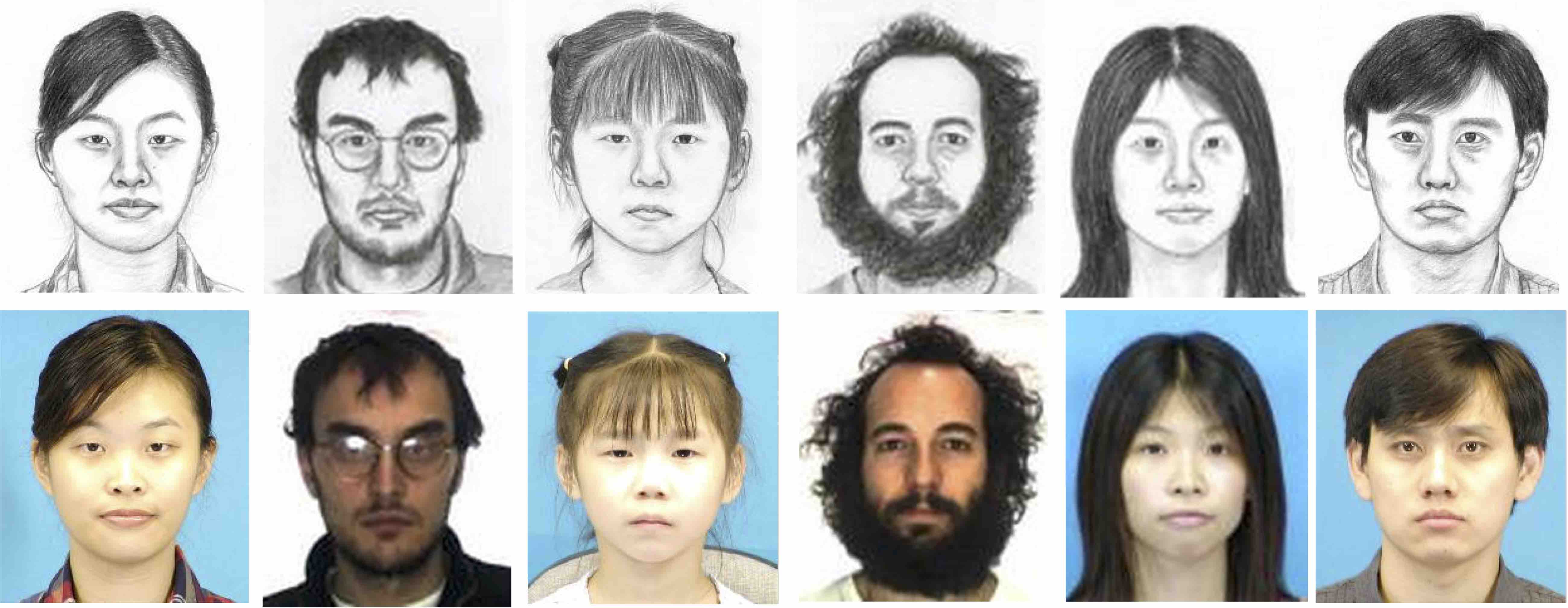
Figure 6: Examples of sketch and face photo pairs of CUFS dataset.

Dataset. We first carried out experiments on sketch to face recognition using the CUFS dataset, a very popular benchmark which contains sketch-face photo pairs collected from 188 CUHK students. Figure 6 shows some examples of sketch-photo pairs. The recognition task is to extract the face photo corresponding to a given sketch as described in Section 4.0.5. We evaluated the performance of our approach on CUFS and compared it to other cross-domain retrieval methods and previous DL approaches.

Settings. Following [54], in our experiments 88 sketch-photo image pairs were randomly selected for training the model, and the remaining 100 pairs were used for testing. To fairly compare with previous works [7, 9], in this preliminary experiment we did not consider the powerful LKS sketch features and CNN image features, but we only used raw pixels as feature representations for the two modalities. We compared the proposed approach with several baseline methods including: canonical correlation analysis (CCA), partial least squares (PLS) [55], bilinear model [56], semi-coupled dictionary learning (SCDL) [8], joint dictionary learning (JDL) [7] and coupled dictionary learning (CDL) [9]. For the bilinear model, we used 70 PLS bases and 50 eigenvectors (see [55]). For all DL-based approaches we set the dictionary size to 50. In all cases, the recognition was performed using the nearest neighbor on the newly learned sparse representation as in [55, 9]. We implemented and evaluated two variants of our method considering two different self-paced regularizers $f_{\textrm{SP}_{A}}$ and $f_{\textrm{SP}_{B}}$ as introduced in Section 3.2. Furthermore, we explicitly evaluated the importance of the relational knowledge ($\beta$) and of self-pacing ($\gamma$). Since for CUFS both sketches and face images are quite homogeneous (i.e. , sketches were drawn by experts, faces in images are centered and equally illuminated), we did not use any curriculum by setting $\mu=0$. The parameters $\alpha$, $\beta$ were set by cross-validation to $1$ and $5$, respectively.

TABLE I: Average recognition rate for all benchmarked methods on CUFS for sketch-to-photo face recognition.

Method	Recognition Rate
Tang & Wang [54]	81.0%
Partial Least Squares (PLS) [55]	93.6%
Biliner model [56]	94.2%
Canonical Correlation Analysis (CCA)	94.6%
Semi-coupled Dictionary Learning (SCDL) [8]	95.2%
Joint Dictionary Learning (JDL) [7]	95.4%
Coupled Dictionary Learning (CDL) [9]	97.4%
CPRL with $f_{\textrm{SP}_{B}}$ ($\beta=\gamma=\mu=0$)	96.8%
CPRL with $f_{\textrm{SP}_{B}}$ ($\gamma=\mu=0$)	97.2%
CPRL with $f_{\textrm{SP}_{A}}$ ($\mu=0$)	98.2%
CPRL with $f_{\textrm{SP}_{B}}$ ($\mu=0$)	98.6%

Results. Table I shows the results of average recognition rate over five trials. CPRL with self-paced regularizer $f_{\textrm{SP}_{B}}$ ($\mu=0$) achieves the best average recognition rate: $98.6\%$ (the influence of different self-paced regularizers is further analyzed in Section 5.4). Remarkably, CPRL with $f_{\textrm{SP}_{B}}$($\mu=0$) outperforms CDL, which is the best of the DL-based approaches, showing the advantage of using our self-paced scheme for learning robust cross-domain representations. Importantly, by setting the parameter $\beta$ to 0, we notice that the effect of the relational knowledge is crucial in the performance of the overall method (CDL also uses relational knowledge). Among the compared methods, SCDL, JDL and CDL are the strongest competitors, achieving $95.2\%$, $95.4\%$ and $97.4\%$ recognition rate respectively. This means that DL is an effective strategy for learning cross-domain representations for the retrieval task. We also remark that CPRL with $f_{\textrm{SP}_{B}}$($\gamma=0$) outperforms the other two versions of CPRL, suggesting that the relational knowledge within the SP learning framework is beneficial for accurate retrieval.

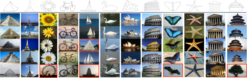
Figure 7: Top 5 retrieval results with sample query sketches in Flickr15K dataset. Red boxes show false positive retrievals.

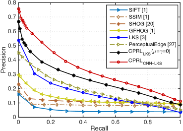
(a) Flickr15K

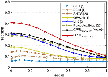
(b) QueenMary SBIR

Figure 8: Precision-Recall (PR) curves for the retrieval performance comparison of the different methods on Flirckr15K and QueenMary SBIR datasets.

5.3 Sketch-to-Image Retrieval

Datasets. We further performed the evaluation of CPRL on the Flickr15k and QueenMary SBIR datasets. The Flickr15k dataset is a widely used dataset for SBIR, containing around 14, 660 images collected from Flickr and 330 free-hand sketches drawn by 10 non-expert sketchers. The dataset consists of 33 object categories and each sample is labeled with an object-class annotation. Since this dataset does not provide a training set, to evaluate our approach, we partitioned the dataset into a training set with randomly chosen 40% samples and a test set with the remaining samples. All the baseline methods were tested using the same setting for a fair comparison.

The Queen Mary SBIR dataset [29] is constructed by intersecting 14 common categories from the Eitz 20,000 sketch dataset [57] and the PASCAL VOC 2010 dataset [58], which consists of 1,120 sketches and 7,267 images. This dataset presents more complex conditions than the Flickr15k due to cluttered background and significant scale variations in the images. We use the official training and testing sets for evaluation. Since this dataset was originally used for fine-grained SBIR, while our task focuses on category-level SBIR, we only used image-level category annotations.

The TU-Berlin Extension dataset [53] consists of 250 object categories and each category has 80 free-hand sketches. Similar to [34], 204,489 extended natural images provided by [59] are added to TU-Berlin image gallery for the retrieval task.

Settings. To demonstrate the retrieval performance of CPRL, we compared with several state of the art SBIR methods, including SHOG [23], SIFT, SSIM, GFHOG evaluated in [1], Structure Tensor [3], Learned Key Shapes as in [4], PerceptualEdge [31], Sketch-a-Net (SaN) [32], Siamese CNN [60], GN Triplet [61], 3D shape [45] and DSH [34]. The first five methods first extract low-level feature representations (SHOG, SIFT, SSIM, GFHOG and StructureTensor) from the Canny edge maps of the images and the sketches respectively, and then generate the corresponding mid-level representations using a bag-of-words approach. Since the Queen Mary SBIR is a more difficult dataset than Flickr15, we considered SP-SHOG and SP-GFHOG instead of SHOG and GFHOG. Indeed, SP-HOG and SP-GFHOG employ a spatial pyramid model over SHOG and GFHOG features which has been demonstrated to provide more robust image representations than BoW [62]. LKS [4] learns mid-level sketch patterns named keyshapes. The learned keyshapes are used to construct image and sketch descriptors. PerceptualEdge [31] uses an edge grouping framework to create synthesized sketches from images. The retrieval is performed by querying the synthesized sketches instead of the images directly. Sketch-a-Net (SaN) [32] is an approach based on recent CNN architectures. Siamese CNN [60] uses a Siamese-based network structure for learning the similarity between the image and the sketch samples. DSH [34] jointly learns a hash function with the front-end CNN. For LKS and PerceptualEdge, we use the original codes provided by the authors with the same parameter setting described in the associated papers and we reimplemented other baselines whose codes are not publicly available. All the methods are evaluated on the same training/testing set for a fair comparison. If the original paper uses the same train/test split, the results are those reported in the paper.

To evaluate the proposed CPRL, we considered several settings using the self-paced regularizer $f_{\textrm{SP}_{B}}$: (i) CPRL${}_{\textsc{LKS}}$ ($\gamma=\mu=0$): CPRL without the curricula and self-pacing, using LKS features for both image and sketch domains; (ii) CPRL${}_{\textsc{LKS}}$: CPRL using LKS features for both the image and the sketch modalities; (iii) CPRL${}_{\textsc{CNN+LKS}}$: CPRL using CNN features for the image domain (i.e. features extracted from the sixth layer of the Caffe reference network trained on ImageNet) and LKS features for the sketch domain. We further considered the last baseline method with self-paced regularizer $f_{\textrm{SP}_{A}}$. The sketch curriculum, when used, is constructed using $60\%$ of human annotations, since we did not observe any significant differences between the automatic and the manual procedures (see Section 5.4). For all CPRL methods, we set $\alpha,\beta,\gamma$ and $N$ with cross-validation, and obtained $\alpha=2$, $\beta=25$, $\gamma=0.5$ and $N=1000$ for Flickr15k, and $\alpha=6$, $\beta=8$, $\gamma=1$ and $N=1500$ for Queen Mary SBIR.

Figure 9: Top 5 retrieved images (right) using the query sketch samples (left) in the QueenMary SBIR dataset. Red boxes show false positive retrievals.

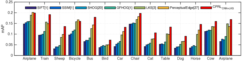
Figure 10: Retrieval performance comparison for each category of the Queen Mary SBIR dataset.

TABLE II: Comparison of different methods on Flickr15k and Queen Mary SBIR datasets

Method	mAP
	Flick15k	QueenMary SBIR
StructureTensor [3]	0.0801	0.0601
SIFT [1]	0.0967	0.0685
SSIM [1]	0.1068	0.0745
SHOG [23]	0.1152	0.0804
GFHOG [1]	0.1245	0.0858
LKS [4]	0.1640	0.1182
PerceptualEdge [31]	0.1741	0.1246
SaN [32]	0.1730	0.1211
Siamese CNN [60]	0.1954	-
CPRL${}_{\textsc{GFHOG}}$ with $f_{\textrm{SP}_{B}}$	0.1693	0.1103
CPRL${}_{\textsc{LKS}}$ with $f_{\textrm{SP}_{B}}$ ($\gamma=\mu=0$)	0.2278	0.1265
CPRL${}_{\textsc{LKS}}$ with $f_{\textrm{SP}_{B}}$	0.2495	0.1467
CPRL${}_{\textsc{CNN+LKS}}$ with $f_{\textrm{SP}_{A}}$	0.2659	0.1521
CPRL${}_{\textsc{CNN+LKS}}$ with $f_{\textrm{SP}_{B}}$	0.2734	0.1603

TABLE III: Comparison of different methods on the TU-Berlin Extension dataset.

Method	Feature Dimension	mAP
SHOG [23]	1296	0.091
GFHOG [1]	3500	0.119
SHELO [2]	1296	0.123
LKS [4]	1350	0.157
SaN [32]	512	0.154
Siamese CNN [60]	64	0.322
GN Triplet [61]	1024	0.187
3D shape [45]	64	0.054
DSH [34]	32 (bits)	0.358
DSH [34]	128 (bits)	0.570
CPRL${}_{\textsc{LKS}}$ with $f_{\textrm{SP}_{B}}$ ($\gamma=\mu=0$)	1000	0.269
CPRL${}_{\textsc{LKS}}$ with $f_{\textrm{SP}_{B}}$	1000	0.301
CPRL${}_{\textsc{CNN+LKS}}$ with $f_{\textrm{SP}_{A}}$	1000	0.324
CPRL${}_{\textsc{CNN+LKS}}$ with $f_{\textrm{SP}_{B}}$	1000	0.332

Results. A performance comparison of different methods on the Flickr15k and the QueenMary SBIR datasets is shown in Table II, reporting the mean average precision (mAP), and in Figure 8, depicting the precision-recall (PR) curve. Analyzing results on the Flickr15K dataset, three observations can be made: (i) CPRL${}_{\textsc{CNN+LKS}}$ achieves the best mAP, showing a significant performance improvement (9.93 points) compared to the best state of the art method ($0.1741$ of PerceptualEdge [31]); (ii) CPRL${}_{\textsc{GFHOG}}$ and CPRL${}_{\textsc{LKS}}$ compares favorably to GFHOG [1] and LKS [4] with $4.48$ and $8.55$ points improvement respectively, meaning that the advantage of the academic learning paradigm and its instantiation under the framework of dictionary learning is clear and independent of the features used; (iii) The clear performance gap when CPRL${}_{\textsc{LKS}}$ is compared to CPRL${}_{\textsc{LKS}}$ ($\gamma=\mu=0$) demonstrates the effectiveness of the proposed CPPCL strategy.

The fact that the best performance is obtained with CPRL${}_{\textsc{CNN+LKS}}$ confirms our original intuition that different features can represent better the two different modalities. Interestingly the results in the table also show that our approach outperforms the SaN method [32] and Siamese CNN method [60], demonstrating the effectiveness of our framework in comparison with deep learning architectures. Finally, Figure 7 shows some qualitative results (top-five retrieved images) associated with the proposed method.

On the Queen Mary SBIR dataset, Table II, CPRL${}_{\textsc{CNN+LKS}}$ achieves an mAP of 0.1603 which is 3.57 points better than the best of all the comparison methods. It should be noted that this is not a trivial improvement on this very challenging dataset. CPRL${}_{\textsc{CNN+LKS}}$ also outperforms CPRL${}_{\textsc{LKS}}$, demonstrating the effectiveness of using different descriptors for sketches and images in SBIR. We also believe that LKS features are not robust enough to represent objects with various poses and cluttered background, as in Queen Mary SBIR dataset. CPRL${}_{\textsc{LKS}}$ obtains a clear improvement over CPRL${}_{\textsc{LKS}}$ ($\gamma=\mu=0$), further verifying the usefulness of the proposed CPPCL scheme. Additionally, we show the retrieval performance for the category-level retrieval task in Figure 10. It is clear that for most of the classes (except for Airplane and Bicycle), CPRL${}_{\textsc{CNN+LKS}}$ significantly outperforms all the comparison methods. Finally, Figure 9 reports the top 5 retrieval results of CPRL${}_{\textsc{CNN+LKS}}$ for 10 query samples of sketches.

We further verify our performance on a larger SBIR dataset TU-Berlin Extension. The results are shown in Table III. It is clear that CPRL${}_{\textsc{LKS}}$ with $f_{\textrm{SP}_{B}}$ is significantly better than the LKS method and CPRL${}_{\textsc{KS}}$ with $f_{\textrm{SP}_{B}}(\gamma=\mu=0)$, demonstrating the effectiveness of the proposed learning strategy. When using powerful CNNs features as input, our method obtains better performance than previous end-to-end trainable deep learning models [32, 60, 61, 45]. The DSH method in [34] achieves the best performance by successfully combining deep networks with hashing. We believe that our learning strategy is complementary to their method and the idea of exploiting curriculum and self-paced learning in the context of deep hashing is an interesting direction for future works.

5.4 In-depth Analysis of CPRL

In this section, we show the results of a further analysis of the proposed CPRL model on both the Flickr15k and the Queen Mary SBIR datasets. The analysis was conducted considering several aspects including sensitivity study, convergence analysis, effect of self-paced regularizers, impact of the curriculum construction and computational cost analysis.

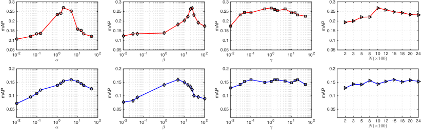
Figure 11: Empirical analysis of the model parameters: $\alpha$, $\beta$, $\gamma$ and the dictionary size $N$ on Flickr15k (first row) and Queen Mary SBIR (second row) datasets.

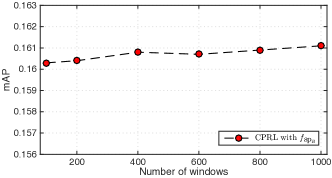
Figure 12: mAP at varying number of windows for edgeness calculation on the Queen Mary SBIR dataset.

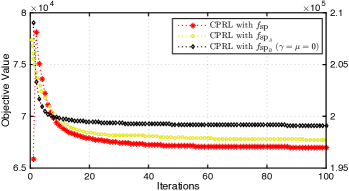
Figure 13: Convergence in terms of objective value for: CPRL with $f_{\textsc{SP}_{A}}$ and with $f_{\textsc{SP}_{B}}$ and CPRL with $f_{\textsc{SP}_{B}}$ ($\gamma=\mu=0$).

Sensitivity analysis. First, we assess the influence in performance of the different model parameters in CPRL. Figure 11 shows the mAP as a function of the parameters $\alpha,\beta,\gamma,N$ on both the Flickr15k and the Queen Mary SBIR datasets. The analysis on $\alpha,\beta$ and $\gamma$ is in the range $[10^{-2},10^{2}]$, on $N$ in the range $[200,2400]$. It is clear from the plots that, while the method is sensitive to $\alpha$ and $\beta$, its retrieval performance does not change drastically within a wide range of $\gamma$ and $N$. The sensitivity on $\beta$ was already observed in previous research works [9]. The performance trend varying the different parameters shows some similarity on both datasets. We also conduct an analysis to evaluate the impact on the performance of the number of windows used for the edgeness calculation in the sketch domain (Fig. 12). Fig. 12 shows that the retrieval performance only slightly improves when increasing the number of windows. However, a large number of windows leads to a significant increase in terms of computational overhead. Therefore, we set the number of windows equal to 100 in our experiments as it represents a good trade-off between accuracy and computational cost.

Convergence analysis. Figure 13 plots the objective function value as a function of the iteration number for the proposed CPRL on Flickr15K with three different settings: (i) CPRL with $f_{\textrm{SP}_{A}}$; (ii) CPRL with $f_{\textrm{SP}_{B}}$ and (iii) CPRL with $f_{\textrm{SP}_{B}}$ ($\gamma=\mu=0$). The results clearly show the convergence of the proposed iterative optimization procedure. All the three settings of CPRL attain a stable solution within less than 40 iterations, proving the efficiency of the algorithm proposed to solve the CPRL optimization problem. It is worth noting that both CPRL with $f_{\textrm{SP}_{A}}$ and with $f_{\textrm{SP}_{B}}$ obtain a much lower local minima than CPRL ($\gamma=\mu=0$) (e.g.  with $f_{\textrm{SP}_{B}}$ giving $6.8\times 10^{4}$ vs. $1.98\times 10^{5}$), verifying the beneficial effect of the proposed CPPCL strategy for better optimization.

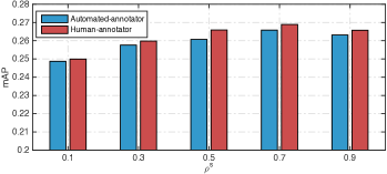
Figure 14: Performance considering automatically obtained and human-annotated sketch partial curricula.

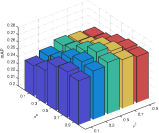
Figure 15: Performance at varying the constraints ratio of the sketch and the image modalities.

Analysis of self-paced regularizers. We carried out the retrieval experiments for CPRL with two different self-paced regularizers $f_{\textrm{SP}_{A}}$ and $f_{\textrm{SP}_{B}}$ on the four datasets. Table I and Table II show the quantitative results of the two CPRL variants. We can observe that CPRL with $f_{\textrm{SP}_{B}}$ slightly outperforms CPRL with $f_{\textrm{SP}_{A}}$ on all the four datasets. We believe that this is probably due to the fact that when we optimize CPRL with $f_{\textrm{SP}_{B}}$, the self-pacing variables $\mathbf{V}$ are relaxed considering a real valued range [0, 1] (i.e.  using a soft-weighting scheme) instead of discrete values. The soft weighting scheme is more effective than the hard weighting one in reflecting the true importance of samples in the training phase. This effect was previously observed in [37, 38].

Analysis of curriculum construction. To investigate the influence the modalitiy-specific curricula to the final retrieval performance, we plot the mAP as a function of $\rho^{\textsc{i}}$ and $\rho^{\textsc{s}}$, the proportion of constraints used for the image and sketch curriculum relative to the number of possible constraints. Figure 15 shows the plot with $\rho^{\textsc{i}}$ and $\rho^{\textsc{s}}$ taking five values ranging from 0.1 to 0.9. We can observe that for both modalities, the use of the curricula indeed helps boosting the performance, while using the excess of constraints leads to a slight decrease in performance. This experimental finding supports our motivation of designing partial curricula learning in CPRL for SBIR. Our CPCL approach allows the human and the automated annotator to construct the partial curricula. To evaluate the difference of these two, Figure 14 plots the mAP as a function of $\rho^{\textsc{s}}$ with $\rho^{\textsc{i}}$ fixed to be 0.3. It is clear that the human annotations correspond to more effective partial curricula, but yet the difference when compared with the automated curricula constructions is small.

Computational cost analysis. In the following, we analyze the computational time overhead on Flickr15K experiments both in the off-line training phase and during the online retrieval phase. The training phase of our method mainly contains three steps: (i) feature extraction, (ii) curriculum construction and (iii) CPRL optimization. The input for CPRL are CNN features (for images) with size $4883\times 2400$ and LKS features (for sketches) with size $132\times 2400$, where $4833$ and $132$ are the number of training image and sketch samples respectively, and $2400$ is the feature dimension. Table IV reports computational times of different steps of the method. For the feature extraction, we consider CNN features from the image domain, which cost around $0.04$ seconds per image sample. The CNN image features were extracted with the GPU. LKS is used to extract features from the sketch domain. The automated curriculum construction takes around $8$ minutes and training CPRL and CPRL ($\gamma=\mu=0$) with $50$ iterations costs $27$ and $21$ minutes, respectively.

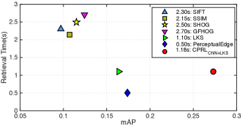
Figure 16: Comparison of the average retrieval time of different methods with respect to the mAP.

TABLE IV: Computational cost of the different training steps.

Phase	Component	Time overhead
Feature Extraction	CNN (for images)	0.04 $\pm$ 0.01 sec/sample
	LKS (for sketches)	1.1 $\pm$ 0.02 sec/sample
Training	Curriculum Construction	8 $\pm$ 1 min
	CPRL	27 $\pm$ 2 min
	CPRL($\gamma=\mu=0$)	21$\pm$ 2 min
Retrieval	CPRL	1.1 $\pm$ 0.1 sec/sample

Online retrieval efficiency is a very important performance index for SBIR, especially for large-scale retrieval scenarios. Figure 16 plots the online retrieval time with respect to the mAP and compares CPRL with the state-of-the-art SBIR methods. Our CPRL${}_{\textsc{CNN+LKS}}$ is based on three steps for the retrieval: (i) feature extraction from a query sketch sample using LKS, (ii) dictionary mapping to obtain a new feature representation and (iii) query the image features database with $k\textsc{-NN}$. The last two steps are very fast, and the feature extraction using LKS takes around 1 second. The average retrieval time for each query sample is around 1.18 seconds. PerceptualEdge method achieves the best retrieval speed, as it uses only two steps namely the HOG feature extraction and direct matching. The retrieval speed of ours is comparable to the LKS method, and is almost 2 times faster than GFHOG, SHOG, SIFT and SSIM, which first extract features, and then construct bag-of-words descriptors and finally perform the retrieval. The reason is that the step of constructing the bag-of-words features is more time consuming than the dictionary mapping step. More importantly, our approach obtains a very good balance between the retrieval performance (mAP) and the computational efficiency.

To conclude, our approach achieves better or comparable speed than previous works based on direct feature matching. We believe that other strategies can be used to further speed up the retrieval process, such as adopting hash-based algorithms. While this is not the focus of the current paper, our framework can be also extended in this direction.

6 Conclusions

We presented a novel cross-domain representation learning framework for computing robust cross-modal features for sketch-based image retrieval. In particular, this work explores self-paced and curriculum learning schemes for dictionary learning. A novel cross-paced partial curriculum learning strategy is designed to learn from samples with an easy-to-hard order, such as to avoid bad local optimal into dictionary learning optimization. The proposed framework naturally handles different descriptors for the sketch and the image domains. Therefore, domain-specific discriminative feature representations (e.g. , CNN features for images) are considered, overcoming the limitations of previous works. Extensive evaluation on four publicly available datasets shows that our approach achieves very competitive performance over state-of-the art methods for SBIR.

In this paper CPPCL is instantiated within a coupled dictionary learning model for addressing the SBIR task. However, CPPCL is a general strategy which can be also combined with other representation learning methods. Future works will explore the adoption of CPPCL into deep cross-domain [63] and deep structured learning models [64].

Dan Xu is a Ph.D. candidate in the Department of Information Engineering and Computer Science, and a member of Multimedia and Human Understanding Group (MHUG) led by Prof. Nicu Sebe at the University of Trento. He was a research assistant in the Multimedia Laboratory in the Department of Electronic Engineering at the Chinese University of Hong Kong. His research focuses on computer vision, multimedia and machine learning. Specifically, he is interested in deep learning, structured prediction and cross-modal representation learning and the applications to scene understanding tasks. He received the Intel best scientific paper award at ICPR 2016.

Xavier Alameda-Pineda received the M.Sc. degree in mathematics and telecommunications engineering from the Universitat Politecnica de Catalunya BarcelonaTech in 2008 and 2009 respectively, the M.Sc. degree in computer science from the Universite Joseph Fourier and Grenoble INP in 2010, and the Ph.D. degree in mathematics/computer science from the Universite Joseph Fourier in 2013. He worked towards his Ph.D. degree in the Perception Team, at INRIA Grenoble Rhone-Alpes. He currently holds a postdoctoral position at the Multimodal Human Understanding Group at University of Trento. His research interests are machine learning and signal processing for scene understanding, speaker diaritzation and tracking, sound source separation and behavior analysis.

Jingkuan Song received the B.S. degree in computer science from the University of Electronic Science and Technology of China and the Ph.D. degree in information technology from The University of Queensland, Australia, in 2014. He is currently a Post-Doctoral Research Scientist with Columbia University. He joined the University of Trento as a Research Fellow sponsored by Prof. Nicu Sebe from 2014-2016. His research interest includes large-scale multimedia retrieval, image/video segmentation, and image/video annotation using hashing, graph learning, and deep learning techniques.

Elisa Ricci received the PhD degree from the University of Perugia in 2008. She is an assistant professor at the University of Perugia and a researcher at Fondazione Bruno Kessler. She has since been a post-doctoral researcher at Idiap, Martigny, and Fondazione Bruno Kessler, Trento. She was also a visiting researcher at the University of Bristol. Her research interests are mainly in the areas of computer vision and machine learning. She is a member of the IEEE.

Nicu Sebe is Professor with the University of Trento, Italy, leading the research in the areas of multimedia information retrieval and human behavior understanding. He was the General Co- Chair of the IEEE FG Conference 2008 and ACM Multimedia 2013, and the Program Chair of the International Conference on Image and Video Retrieval in 2007 and 2010, ACM Multimedia 2007 and 2011. He is the Program Chair of ICCV 2017 and ECCV 2016, and a General Chair of ACM ICMR 2017 and ICPR 2020. He is a fellow of the International Association for Pattern Recognition.

References

- [1] R. Hu and J. Collomosse, “A performance evaluation of gradient field hog descriptor for sketch based image retrieval,” CVIU, vol. 117, no. 7, pp. 790–806, 2013.
- [2] J. M. Saavedra, “Sketch based image retrieval using a soft computation of the histogram of edge local orientations (s-helo),” in ICIP, 2014.
- [3] M. Eitz, K. Hildebrand, T. Boubekeur, and M. Alexa, “An evaluation of descriptors for large-scale image retrieval from sketched feature lines,” Computers & Graphics, vol. 34, no. 5, pp. 482–498, 2010.
- [4] J. M. Saavedra, J. M. Barrios, and S. Orand, “Sketch based image retrieval using learned keyshapes (LKS),” in BMVC, 2015.
- [5] J. M. Saavedra and B. Bustos, “An improved histogram of edge local orientations for sketch-based image retrieval,” in Pattern Recognition. Springer, 2010, pp. 432–441.
- [6] H. Lee, A. Battle, R. Raina, and A. Y. Ng, “Efficient sparse coding algorithms,” in NIPS, 2006.
- [7] J. Yang, J. Wright, T. S. Huang, and Y. Ma, “Image super-resolution via sparse representation,” TIP, vol. 19, no. 11, pp. 2861–2873, 2010.
- [8] S. Wang, L. Zhang, Y. Liang, and Q. Pan, “Semi-coupled dictionary learning with applications to image super-resolution and photo-sketch synthesis,” in CVPR, 2012.
- [9] D.-A. Huang and Y.-C. F. Wang, “Coupled dictionary and feature space learning with applications to cross-domain image synthesis and recognition,” in ICCV, 2013.
- [10] F. Feng, X. Wang, and R. Li, “Cross-modal retrieval with correspondence autoencoder,” in ACM MM, 2014.
- [11] B. Wang, Y. Yang, X. Xu, A. Hanjalic, and H. T. Shen, “Adversarial cross-modal retrieval,” in ACM MM, 2017, pp. 154–162.
- [12] D. Xu, W. Ouyang, E. Ricci, X. Wang, and N. Sebe, “Learning cross-modal deep representations for robust pedestrian detection,” in CVPR, 2017.
- [13] D. Xu, E. Ricci, W. Ouyang, X. Wang, and N. Sebe, “Multi-scale continuous crfs as sequential deep networks for monocular depth estimation,” in CVPR, 2017.
- [14] M. P. Kumar, B. Packer, and D. Koller, “Self-paced learning for latent variable models,” in NIPS, 2010.
- [15] Y. Bengio, J. Louradour, R. Collobert, and J. Weston, “Curriculum learning,” in ICML, 2009.
- [16] J. S. Supancic and D. Ramanan, “Self-paced learning for long-term tracking,” in CVPR, 2013.
- [17] Y. J. Lee and K. Grauman, “Learning the easy things first: Self-paced visual category discovery,” in CVPR, 2011.
- [18] L. Jiang, D. Meng, Q. Zhao, S. Shan, and A. G. Hauptmann, “Self-paced curriculum learning,” in AAAI, 2015.
- [19] D. Xu, X. Alameda-Pineda, J. Song, E. Ricci, and N. Sebe, “Academic coupled dictionary learning for sketch-based image retrieval,” in ACM MM, 2016.
- [20] T. Kato, T. Kurita, N. Otsu, and K. Hirata, “A sketch retrieval method for full color image database-query by visual example,” in ICPR, 1992.
- [21] A. Chalechale, G. Naghdy, and A. Mertins, “Sketch-based image matching using angular partitioning,” TSMC, vol. 35, no. 1, pp. 28–41, 2005.
- [22] A. D. Bimbo and P. Pala, “Visual image retrieval by elastic matching of user sketches,” TPAMI, vol. 19, no. 2, pp. 121–132, 1997.
- [23] M. Eitz, K. Hildebrand, T. Boubekeur, and M. Alexa, “Sketch-based image retrieval: Benchmark and bag-of-features descriptors,” TVCG, vol. 17, no. 11, pp. 1624–1636, 2011.
- [24] X. Cao, H. Zhang, S. Liu, X. Guo, and L. Lin, “Sym-fish: A symmetry-aware flip invariant sketch histogram shape descriptor,” in ICCV, 2013.
- [25] D. G. Lowe, “Object recognition from local scale-invariant features,” in ICCV, 1999.
- [26] N. Dalal and B. Triggs, “Histograms of oriented gradients for human detection,” in CVPR, 2005.
- [27] X. Sun, C. Wang, C. Xu, and L. Zhang, “Indexing billions of images for sketch-based retrieval,” in ACM MM, 2013.
- [28] Y.-L. Lin, C.-Y. Huang, H.-J. Wang, and W.-C. Hsu, “3d sub-query expansion for improving sketch-based multi-view image retrieval,” in ICCV, 2013.
- [29] Y. Li, T. M. Hospedales, Y.-Z. Song, and S. Gong, “Fine-grained sketch-based image retrieval by matching deformable part models,” in BMVC, 2014.
- [30] C. Xiao, C. Wang, L. Zhang, and L. Zhang, “Sketch-based image retrieval via shape words,” in ICMR, 2015.
- [31] Y. Qi, Y.-Z. Song, T. Xiang, H. Zhang, T. Hospedales, Y. Li, and J. Guo, “Making better use of edges via perceptual grouping,” in CVPR, 2015.
- [32] Q. Yu, Y. Yang, Y.-Z. Song, T. Xiang, and T. Hospedales, “Sketch-a-net that beats humans,” in BMVC, 2015.
- [33] Q. Yu, F. Liu, Y.-Z. Song, T. Xiang, T. M. Hospedales, and C.-C. Loy, “Sketch me that shoe,” in CVPR, 2016.
- [34] L. Liu, F. Shen, Y. Shen, X. Liu, and L. Shao, “Deep sketch hashing: Fast free-hand sketch-based image retrieval,” in CVPR, 2017.
- [35] K. Wang, R. He, W. Wang, L. Wang, and T. Tan, “Learning coupled feature spaces for cross-modal matching,” in ICCV, 2013.
- [36] P. Xu, Q. Yin, Y. Qi, Y.-Z. Song, Z. Ma, L. Wang, and J. Guo, “Instance-level coupled subspace learning for fine-grained sketch-based image retrieval,” in ECCV, 2016.
- [37] Q. Zhao, D. Meng, L. Jiang, Q. Xie, Z. Xu, and A. G. Hauptmann, “Self-paced learning for matrix factorization,” in AAAI, 2015.
- [38] C. Xu, D. Tao, and C. Xu, “Multi-view self-paced learning for clustering,” in IJCAI, 2015.
- [39] A. Pentina, V. Sharmanska, and C. H. Lampert, “Curriculum learning of multiple tasks,” in CVPR, 2015.
- [40] Y. Tang, Y.-B. Yang, and Y. Gao, “Self-paced dictionary learning for image classification,” in ACM MM, 2012.
- [41] L. Jiang, D. Meng, T. Mitamura, and A. G. Hauptmann, “Easy samples first: Self-paced reranking for zero-example multimedia search,” in ACM MM, 2014.
- [42] L. Jiang, D. Meng, S.-I. Yu, Z. Lan, S. Shan, and A. Hauptmann, “Self-paced learning with diversity,” in NIPS, 2014.
- [43] J. Mairal, F. Bach, J. Ponce, G. Sapiro, and A. Zisserman, “Non-local sparse models for image restoration,” in ICCV, 2009.
- [44] Y. Yan, Y. Yang, H. Shen, D. Meng, G. Liu, A. Hauptmann, and N. Sebe, “Complex event detection via event oriented dictionary learning,” in AAAI, 2015.
- [45] F. Wang, L. Kang, and Y. Li, “Sketch-based 3d shape retrieval using convolutional neural networks,” in CVPR, 2015.
- [46] J. Guo, C. Wang, and H. Chao, “Building effective representations for sketch recognition,” in AAAI, 2015.
- [47] J. Ngiam, A. Khosla, M. Kim, J. Nam, H. Lee, and A. Y. Ng, “Multimodal deep learning,” in ICML, pp. 689–696.
- [48] X. Wang and X. Tang, “Face photo-sketch synthesis and recognition,” TPAMI, vol. 31, no. 11, pp. 1955–1967, 2009.
- [49] X. Zhai, Y. Peng, and J. Xiao, “Heterogeneous metric learning with joint graph regularization for cross-media retrieval,” in AAAI, 2013.
- [50] B. Alexe, T. Deselaers, and V. Ferrari, “Measuring the objectness of image windows,” TPAMI, vol. 34, no. 11, pp. 2189–2202, 2012.
- [51] A. Beck and M. Teboulle, “A fast iterative shrinkage-thresholding algorithm for linear inverse problems,” SIAM J. Imag. Sciences, vol. 2, no. 1, pp. 183–202, 2009.
- [52] R. J. Vanderbei, “Loqo: An interior point code for quadratic programming,” Optimization methods and software, vol. 11, no. 1-4, pp. 451–484, 1999.
- [53] M. Eitz, J. Hays, and M. Alexa, “How do humans sketch objects?” TOG, vol. 31, no. 4, pp. 44–1, 2012.
- [54] X. Tang and X. Wang, “Face sketch recognition,” TCSVT, vol. 14, no. 1, pp. 50–57, 2004.
- [55] A. Sharma and D. W. Jacobs, “Bypassing synthesis: Pls for face recognition with pose, low-resolution and sketch,” in CVPR, 2011.
- [56] J. B. Tenenbaum and W. T. Freeman, “Separating style and content with bilinear models,” Neural Computation, vol. 12, no. 6, pp. 1247–1283, 2000.
- [57] M. Eitz, J. Hays, and M. Alexa, “How do humans sketch objects?” TOG, vol. 31, no. 4, p. 44, 2012.
- [58] M. Everingham, L. Van Gool, C. K. Williams, J. Winn, and A. Zisserman, “The pascal visual object classes (VOC) challenge,” IJCV, vol. 88, no. 2, pp. 303–338, 2010.
- [59] H. Zhang, S. Liu, C. Zhang, W. Ren, R. Wang, and X. Cao, “Sketchnet: Sketch classification with web images,” in CVPR, 2016.
- [60] Y. Qi, Y.-Z. Song, H. Zhang, and J. Liu, “Sketch-based image retrieval via siamese convolutional neural network,” in ICIP, 2016.
- [61] P. Sangkloy, N. Burnell, C. Ham, and J. Hays, “The sketchy database: learning to retrieve badly drawn bunnies,” TOG, vol. 35, no. 4, p. 119, 2016.
- [62] S. Lazebnik, C. Schmid, and J. Ponce, “Beyond bags of features: Spatial pyramid matching for recognizing natural scene categories,” in CVPR, 2006.
- [63] D. Xu, E. Ricci, Y. Yan, J. Song, and N. Sebe, “Learning deep representations of appearance and motion for anomalous event detection,” in BMVC, 2015.
- [64] D. Xu, W. Ouyang, X. Alameda-Pineda, E. Ricci, X. Wang, and N. Sebe, “Learning deep structured multi-scale features using attention-gated crfs for contour prediction,” in NIPS, 2017.