Nested Quantum Annealing Correction at Finite Temperature: $p$-spin models

Abstract

Quantum annealing in a real device is necessarily susceptible to errors due to diabatic transitions and thermal noise. Nested quantum annealing correction is a method to suppress errors by using an all-to-all penalty coupling among a set of physical qubits representing a logical qubit. We show analytically that nested quantum annealing correction can suppress errors effectively in ferromagnetic and antiferromagnetic Ising models with infinite-range interactions. Our analysis reveals that the nesting structure can significantly weaken or even remove first-order phase transitions, in which the energy gap closes exponentially. The nesting structure also suppresses thermal fluctuations by reducing the effective temperature.

I Introduction

There has been much interest in developing methods based on quantum mechanics to solve classically hard problems. Among such methods, quantum annealing (QA) emerged as a quantum metaheuristic to solve hard optimization problems Finnila et al. (1994); Kadowaki and Nishimori (1998); Farhi et al. (2001); Brooke et al. (1999, 2001); Santoro et al. (2002); Das and Chakrabarti (2008); Farhi et al. (2001). The algorithm attempts to find a configuration of variables that minimize a cost function, or a problem Hamiltonian, by carefully exploiting the effects of quantum fluctuations. As such, a physical implementation of the algorithm in quantum hardware is of particular interest, since it might lead to quantum speedups over algorithms running on classical hardware. Following pioneering QA experiments in naturally occurring disordered magnets Brooke et al. (1999, 2001), theoretical proposals Kaminsky and Lloyd (2004); Kaminsky et al. (2004) inspired the construction of commercial, programmable quantum annealing processors using superconducting flux qubits by D-Wave Systems Inc. Harris et al. (2010a, b); Berkley et al. (2010); Johnson et al. (2011); Berkley et al. (2013); Bunyk et al. (Aug. 2014); Lanting et al. (2014); Dickson et al. (2013). These processors implement the transverse field Ising model and have been the subject of intense independent scrutiny Boixo et al. (2013, 2014); Albash et al. (2015a, b); Smolin and Smith (2014); Wang et al. (2013); Shin et al. (2014a, b), as the search for examples of quantum speedup using them continues Rønnow et al. (2014); Boixo et al. (2016); Venturelli et al. (2015); King et al. (2017); McGeoch and Wang (2013); King et al. (2015); Hen et al. (2015); Katzgraber et al. (2015); McGeoch and Wang (2013); Denchev et al. (2016); Mandrà et al. (2016); King et al. (2015); Vinci and Lidar (2016); Albash and Lidar (2017); Mandrà and Katzgraber (2017). They have also inspired alternative approaches to QA with more coherent but far less numerous flux qubits Yan et al. (2016); Weber et al. (2017). Alternative approaches that implement the transverse field Ising model using atomic systems such as ion traps Islam et al. (2013); Smith et al. (2016), quantum gas microscopes Simon et al. (2011); Boll et al. (2016), and Rydberg atoms Weimer et al. (2010); Nguyen et al. (2017) are also being actively pursued, primarily for the purpose of quantum simulation of interacting quantum spin systems, but such systems are likely to be flexible enough to also be used eventually for solving combinatorial optimization problems, and have already broken the $50$ qubit barrier Bernien et al. (2017); Zhang et al. (2017).

The idea of using quantum hardware to realize algorithmic speedups of course has deep roots in quantum computation Feynman (1985); R.P. Feynman (1982), which provided the first theoretical examples of quantum speedups D. Deutsch and R. Jozsa (1992); E. Bernstein and U. Vazirani (1993); Shor (20-22 Nov 1994); Grover (1996). Adiabatic quantum computing (AQC), or the quantum adiabatic algorithm Farhi et al. (2000, 2001), is a QA-inspired idea that formalizes the requirements for a quantum speedup using the quantum adiabatic theorem Born and Fock (1928); Kato (1950). This theorem (or set of theorems Garrido and Sancho (1962); Nenciu (1980); Avron et al. (1987); Hagedorn and Joye (2002); Jansen et al. (2007); Lidar et al. (2009); Ge et al. (2016); Bachmann et al. (2017)) guarantees that the minimum of a problem Hamiltonian can be found by an adiabatic process in a closed system, provided the computational time grows inversely with a small power (typically $2$ or $3$) of the minimum gap encountered during the adiabatic evolution. If this gap closes more slowly with the problem size than the best classical algorithm for the same problem, then the adiabatic algorithm provides a quantum speedup; otherwise it may result in a slowdown (the adiabatic theorem only provides a sufficient condition). Examples of both types of scenarios are known and have been reviewed in Ref. Albash and Lidar (2016).

Just like any other quantum information processing method, the performance of real quantum annealers is hindered by decoherence and control errors. The former are due to the presence of the omnipresent (thermal) bath interacting with the physical device, and the latter are due to the analog nature of the computation. Therefore, the development of error correction techniques is crucial for the scalability and ultimate usefulness of QA hardware. Various error suppresion methods for AQC have been proposed and studied theoretically Jordan et al. (2006); Quiroz and Lidar (2012); Young et al. (2013a); Sarovar and Young (2013); Young et al. (2013b); Bookatz et al. (2015); Marvian and Lidar (2014); Jiang and Rieffel (2017); Marvian (2016); Marvian and Lidar (2017); Lidar (2008); Ganti et al. (2014). An error correction approach that can be directly implemented on the current generations of quantum annealers, called quantum annealing correction (QAC), has been developed and tested experimentally Pudenz et al. (2014, 2015); Mishra et al. (2015); Vinci et al. (2015, 2016); Vinci and Lidar (2017).

In QAC, logical qubits are redundantly encoded into a larger number of physical qubits. Energy penalties which commute with the problem Hamiltonian but anticommute with undesired spin-flips occurring late in the computation (errors) are then introduced in order to induce the physical qubits representing each logical variable to represent it consistently throughout the anneal. At the end of the anneal a decoding procedure is performed, which enables the recovery of logical ground-state candidates even if errors did accumulate during the anneal and the final state is not in the code space. Three types of QAC have been introduced and studied. The first uses designated penalty qubits to impose the energy penalty Pudenz et al. (2014, 2015); Mishra et al. (2015) [which we refer to as “penalty QAC” (PQAC)], while the other two use no designated penalty qubits but connect physical qubits to impose penalties against excitations Vinci et al. (2015, 2016); Vinci and Lidar (2017). Of these, one uses a two-level grid structure to connect physical qubits Vinci et al. (2015), while the other uses a nesting of complete graphs for this purpose. Here we are primarily interested in the latter, known as “nested QAC” (NQAC). Experiments using four different generations of the D-Wave quantum annealing devices show that all three methods increase the success probability of QA significantly Pudenz et al. (2014, 2015); Vinci et al. (2015); Mishra et al. (2015); Vinci et al. (2016); Vinci and Lidar (2017). In one case the scaling of the time-to-solution in the case of random Ising problems was shown to improve using PQAC Pudenz et al. (2015), which to date is the only demonstration of error correction improving the algorithmic performance of a quantum information processing device.

Previously, we used a mean field analysis to study the performance of PQAC for the transverse field Ising model in both the ferromagnetic and Hopfield model cases, the latter involving randomness and frustration Matsuura et al. (2016, 2017). We showed analytically that PQAC can prevent or ‘soften’ a quantum phase transition, depending on its order. In PQAC, the designated penalty qubits behave as a source of external fields. At zero temperature, this makes the paramagnetic phase unstable and induces symmetry breaking from the paramagnetic phase to the ferromagnetic or Hopfield phase. At finite temperature, the paramagnetic phase is not destabilized by the penalty term. Nevertheless, the effective free energy barrier between the two phases becomes significantly smaller as the penalty coupling increases, thus enhancing tunneling.

Here, we use the same approach to analytically study NQAC at zero and finite temperatures. Because of the high connectivity in NQAC, the mean field approach is particularly suitable.

The remainder of this paper is organized as follows. We first review NQAC in Sec. II. In Sec. III, we study the phase diagrams of ferromagnetic systems after NQAC by analyzing the free energy and saddle point equations. We show how NQAC changes the properties of phase transitions depending on the type of interactions. In Sec. V, we study the antiferromagnetic case. Section VI discusses the effect of introducing designated penalty qubits in NQAC. We conclude with a discussion in Sec. VII. Details of various calculations and additional results are given in the Appendix.

II Hamiltonian for nested quantum annealing correction

Many combinatorial optimization problems can be formulated in terms of a classical Ising Hamiltonian Lucas (2014),

$$H^{Z}=-\sum_{i}h_{i}\sigma^{z}_{i}-\sum_{(i,j)}J_{ij}\sigma^{z}_{i}\sigma^{z}_{j}\ ,$$ (1)

where $i=1,2,\dots,N$ are site as well as qubit indices, $\{h_{i}\}$ the local fields, $\{J_{ij}\}$ the Ising couplings, and $\sigma^{\alpha}_{i}$ is the $\alpha\in\{x,y,z\}$-component of the Pauli matrix acting on the $i$-th qubit. The couplings $\{h_{i}\}$ and $\{J_{ij}\}$ are chosen so that the ground state of $H^{Z}$ represents the solution to the optimization problem we wish to solve. Quantum fluctuations are induced by a driver Hamiltonian. We consider the standard form,

$$H^{X}=-\sum_{i=1}^{N}\sigma^{x}_{i}\ ,$$ (2)

whose ground state is easy to prepare, and which has a small but non-vanishing overlap with any eigenstate of $H^{Z}$. The time-dependent Hamiltonian is given by

$$H=A(t)H^{X}+B(t)H^{Z}\equiv B(t)\left(\Gamma(t)H^{X}+H^{Z}\right)\ .$$ (3)

The initial state at $t=0$ is the ground state of the driver Hamiltonian [$A(0)=1,B(0)=0$]. We adiabatically reduce quantum fluctuations to reach the problem Hamiltonian at the final time $t=t_{f}$ [$A(t_{f})=0,B(t_{f})=1$].

Fluctuations induced by the driver term are desirable but are deliberately made less likely towards the end of the anneal by decreasing the magnitude of the driver term. However, undesirable bath-induced fluctuations can cause bit-flip errors at all times, including when $A(t)\ll B(t)$, which generally result in transitions out of the ground state. To reduce the likelihood of such undesirable fluctuations we use NQAC to encode the Hamiltonian Vinci et al. (2016). The basic idea is to (1) increase the energy cost of an undesirable bit-flip by creating ferromagnetically coupled logical qubits, (2) decode any bit-flip errors that might have nevertheless taken place.

We label a physical qubit within the $i$-th logical qubit by $(i,c)$, with the logical qubit index $i=1,\cdots,N$ and the nesting index $c=1,\cdots,C$. The physical problem Hamiltonian (1) is first promoted to a logical problem Hamiltonian, whose Pauli matrices $\sigma^{z}_{i}$ represent the logical binary ($\pm 1$) variables of the given optimization problem. All indices in the logical problem Hamiltonian are then mapped to physical qubit indices as $\sigma^{z}_{i}\mapsto\sigma^{z}_{ic}$, $J_{ij}\mapsto J_{(i,c)(j,c^{\prime})}$, and $h_{i}\mapsto h_{(i,c)}$. Logical qubits $i$ and $j$ interact with strength $J_{ij}$. An obvious way to realize this is to connect all physical qubits $(i,c)$ and $(j,c^{\prime})$ with the same strength, and correspondingly rescale the local fields:

$$J_{(i,c),(j,c^{\prime})} =J_{ij},\leavevmode\nobreak\ \leavevmode\nobreak\ \leavevmode\nobreak\ \forall c,c^{\prime}\leavevmode\nobreak\ \leavevmode\nobreak\ \leavevmode\nobreak\ \forall i\neq j$$ (4a)

$$h_{(i,c)} =Ch_{i},\leavevmode\nobreak\ \leavevmode\nobreak\ \leavevmode\nobreak\ \forall c,i\ .$$ (4b)

The need to rescale the local fields by $C$ can be viewed to some extent as a deficiency of NQAC since it requires growing the energy scale; it can of course be avoided by restricting ourselves to problem instances without local fields. Reducing the energy scale by rescaling $J$ to $J/C$ is not necessarily preferable, since in practice, with finite precision couplers as is the case with the current generation of commercial quantum annealers, this means a loss of precision.

Next is the penalty term. In NQAC we couple all $C$ physical qubits of logical qubit $i$ ferromagnetically with strength $\gamma$,

$$J_{(i,c),(i,c^{\prime})}=\gamma,\leavevmode\nobreak\ \leavevmode\nobreak\ \leavevmode\nobreak\ \forall c\neq c^{\prime}\leavevmode\nobreak\ \leavevmode\nobreak\ \leavevmode\nobreak\ \forall i\ ,$$ (5)

so that bit-flip errors are suppressed by an energy gap. As long as no more than $\lfloor(C-1)/2\rfloor$ of the qubits have flipped, we can faithfully decode the logical qubit. In other words, we can equivalently view this procedure as encoding a logical qubit into a distance-$C$ repetition code. The $N$ penalty terms (one for each logical qubit)

$$H_{\mathrm{pen},i}=-\gamma\left(\sum_{c_{i}=1}^{C}\sigma_{ic_{i}}^{z}\right)^{2}=-\gamma\left[CI+2\sum_{c<c^{\prime}}^{C}\sigma_{ic}^{z}\sigma_{ic^{\prime}}^{z}\right]$$ (6)

are added to the total Hamiltonian. Note that this sum includes $C$ identity terms which merely shift the total energy, and that we are double-counting the interactions; the latter means that the physical penalty strength is actually $2\gamma$. Note further that each $\sigma_{ic}^{z}\sigma_{ic^{\prime}}^{z}$ term can be understood as an element of the stabilizer of the distance-$C$ repetition code; because of the complete graph ($K_{C}$) connectivity of the physical qubits, each single-qubit bit-flips error $\sigma^{x}_{ic}$ anticommutes with (is detected by) $C-1$ such terms, which is another way to understand the energy penalty using the ideas of error suppression for AQC Jordan et al. (2006); Quiroz and Lidar (2012); Young et al. (2013a); Sarovar and Young (2013); Young et al. (2013b); Bookatz et al. (2015); Marvian and Lidar (2014); Jiang and Rieffel (2017); Marvian (2016); Marvian and Lidar (2017).

Since current QA devices do not extend control to the driver Hamiltonian, which is fixed as a simple sum over single-qubit $\sigma^{x}$ terms, the new driver Hamiltonian replacing Eq. (2) is simply

$$H^{X}=-\sum_{i=1}^{N}\sum_{c_{i}=1}^{C}\sigma^{x}_{ic_{i}}\ .$$ (7)

Note that this means that the driver Hamiltonian appears as an ‘error’ detected by the penalty Hamiltonian. This is clearly an undesirable aspect of NQAC, but as we shall see it will fortunately not completely spoil the method’s error suppression ability. Intuitively, this can be understood as being due to the fact that the suppression effect is small when fluctuations are deliberate [i.e., when $B(t)\ll A(t)$]. Conversely, the suppression effect peaks when the deliberate fluctuations are small [i.e., when $B(t)\gg A(t)$], and this is exactly when undesirable fluctuations would be potent if left unsuppressed. The potentially problematic regime is when $B(t)\approx A(t)$; our analysis below reveals that the problem is in fact not severe. Finally, note that to also encode the driver Hamiltonian using the logical operators of the repetition code (as in the AQC schemes Jordan et al. (2006); Quiroz and Lidar (2012); Young et al. (2013a); Sarovar and Young (2013); Young et al. (2013b); Bookatz et al. (2015); Marvian and Lidar (2014); Jiang and Rieffel (2017); Marvian (2016); Marvian and Lidar (2017)) would require mapping $\sigma^{x}_{i}\mapsto\otimes_{c=1}^{C}\sigma^{x}_{ic}$, which is unfeasible.

III Second-order transition in the ferromagnetic model

We first consider a mean-field analysis of an NQAC implementation of a fully ferromagnetic system with two-body interactions. As we shall see, this system undergoes a second order phase transition during the anneal. Our analysis in this section reproduces in more detail some of the results first reported in Ref. Vinci et al. (2016).

III.1 Problem formulation and the free energy

We choose the logical problem Hamiltonian to be the infinite-range ferromagnetic Ising model with two-body interactions,

$$H^{Z}=-\frac{J}{N}\left(\sum_{i}\sigma^{z}_{i}\right)^{2}.$$ (8)

The encoded Hamiltonian takes the following form according to Eq. (4),

$$H= -\Gamma H^{X}-{J\over N}\sum_{i\neq j}^{N}\sum_{c_{i},c_{j}=1}^{C}\sigma_{ic_{i}}^{z}\sigma_{jc_{j}}^{z}-\sum_{i=1}^{N}H_{\mathrm{pen},i}$$ (9a)

$$= -\Gamma H^{X}-{NJ}\left({1\over N}\sum_{i=1}^{N}\sum_{c_{i}=1}^{C}\sigma_{ic_{i}}^{z}\right)^{2}$$

$$-\lambda\sum_{i=1}^{N}\left(\sum_{c_{i}=1}^{C}\sigma_{ic_{i}}^{z}\right)^{2}$$ (9b)

where

$$\lambda\equiv\gamma-{J/N}$$ (10)

and from now on $H^{X}$ is as given in Eq. (7). We are interested in the large $N$ limit in this work while keeping $J$ fixed, so that $\gamma\to\lambda$. We shall thus refer to $\lambda$ as the effective penalty strength. Note that in Eq. (9a) we have rescaled the logical couplings, as is customary in mean-field analyses, to ensure that the total Hamiltonian is extensive in $N$. Our goal is to understand the free-energy landscape and the effects of the nesting level $C$ from the point of view of mean field theory.

For a given temperature $T=1/\beta$ and a Hamiltonian $H$, the partition function is given by $Z=\text{tr}\,e^{-\beta H}$ (we use units where $k_{\text{B}}=\hbar=1$). The free energy per single logical qubit is defined by $F=-(T/N)\log Z$. We take the following standard steps. First, we apply the Suzuki-Trotter decomposition Suzuki (1976) to rewrite the partition function in path integral form. Then we introduce Hubbard-Stratonovich fields $m_{i}$ for each logical qubit and $m$ for the total magnetization,

$$S_{i}^{z(x)} =\frac{1}{C}\sum_{c=1}^{C}\sigma_{ic}^{z(x)},\leavevmode\nobreak\ \leavevmode\nobreak\ \leavevmode\nobreak\ S^{z}=\frac{1}{N}\sum_{i=1}^{N}S_{i}^{z}$$ (11a)

$$m_{i} =\left\langle S_{i}^{z}\right\rangle,\leavevmode\nobreak\ \leavevmode\nobreak\ \leavevmode\nobreak\ m=\left\langle S^{z}\right\rangle={1\over N}\sum_{i=1}^{N}m_{i},$$ (11b)

where brackets denote the standard thermal average. We make the static approximation, i.e., we take the fields $m_{i}$ and $m$ to be constant along the Euclidean time direction. This is known to give the exact solution in the case of without nesting ($C=1$) Seoane and Nishimori (2012). The path integral is dominated by its saddle point for $m$ and $m_{i}$ when $N$ and $C$ are large. A practically interesting case is $N\gg C>1$, which corresponds to exploring the effects of NQAC on a computational problem with a large number of logical variables. We expect the mean field approximation within each logical qubit to be reasonably good already for moderately large $C$. By following the steps outlined above (see Appendix A for a detailed derivation) we find that the free energy is given by

$$F =JC^{2}m^{2}+{\lambda C^{2}\over N}\sum_{i=1}^{N}m_{i}^{2}+$$ (12)

$$-{C\over\beta N}\sum_{i=1}^{N}\log\left[2\cosh\left(\beta\sqrt{4C^{2}(Jm+\lambda m_{i})^{2}+\Gamma^{2}}\right)\right]\ .$$

We are interested in extracting the effect of nesting on the physical parameters of the problem. In particular, we would like to determine how $C$ rescales the temperature and the transverse field strength. Note that the quantum effects are captured by the last term in this free energy expression, since it explicitly contains the transverse field through its dependence on $\Gamma$.

III.1.1 The low temperature limit

In the low temperature limit $\beta\to\infty$,

$$F \to JC^{2}m^{2}+{\lambda C^{2}\over N}\sum_{i=1}^{N}m_{i}^{2}+$$ (13)

$$- {1\over N}\sum_{i=1}^{N}\sqrt{4(JC^{2}m+\lambda C^{2}m_{i})^{2}+(\Gamma C)^{2}}.$$ (14)

One can see that, in this low temperature limit, the effect of $C$ levels of nesting is equivalent to rescaling all the parameters appearing in the free energy $F$ as follows:

$$\beta\to\beta,\leavevmode\nobreak\ \leavevmode\nobreak\ J\to JC^{2},\leavevmode\nobreak\ \leavevmode\nobreak\ \lambda\to\lambda C^{2},\leavevmode\nobreak\ \leavevmode\nobreak\ \Gamma\to\Gamma C\,,$$ (16)

which can be interpreted as a boost of the problem couplings by a factor of $C^{2}$ while the driver term is boosted by a factor of $C$ only. The fact that the driver term scales differently than the problem Hamiltonian is due to the aforementioned fact that, in QAC, the driver term is not encoded.

Alternatively, since the partition function is $Z=e^{-N\beta F}$, we can interpret the effect of nesting as being equivalent to the following rescaling

$$\beta\to\beta C^{2}\leavevmode\nobreak\ \leavevmode\nobreak\ J\to J,\leavevmode\nobreak\ \leavevmode\nobreak\ \lambda\to\lambda,\leavevmode\nobreak\ \leavevmode\nobreak\ \Gamma\to\Gamma/C\ .$$ (17)

This can be understood as an effective temperature reduction by a factor of $C^{2}$, although at the same time the driver term is reduced by a factor of $C$, which corresponds to a suppression of quantum fluctuations; this once again reflects the price we have to pay for not encoding the driver Hamiltonian. The problem can be alleviated by rescaling $\Gamma$ to $C\Gamma$ by either increasing $A(t)$ or decreasing $B(t)$ [recall from Eq. (3) that $\Gamma(t)=A(t)/B(t)$], but this presents a problem similar to the one discussed in relation to the rescaling of the local field $h_{i}$ following Eq. (4).

The effective temperature reduction was one of the main conclusions first reported in Ref. Vinci et al. (2016), and we shall expand on it here: it is possible to ‘trade’ physical qubits in exchange for a lower effective temperature. This provides an important mechanism for reducing thermal excitations occurring in physical implementations of quantum annealing. The nested structure of NQAC takes advantage of a more complex encoding to achieve better error correction than PQAC, in which the free energy is only linearly proportional to the number of physical qubits per logical qubit (the parameter $C$ in NQAC) Matsuura et al. (2017).

III.1.2 Arbitrary temperature

We can derive the saddle-point equation for $m_{i}$ directly from Eq. (12) without taking the low temperature limit. The result is:

$$m_{i} = {2(Jm+\lambda m_{i})\over\sqrt{4(Jm+\lambda m_{i})^{2}+(\Gamma/C)^{2}}}$$ (18)

$$\times \tanh\left[(\beta C)\sqrt{4(Jm+\lambda m_{i})^{2}+(\Gamma/C)^{2}}\right].$$ (19)

This shows that the effect of nesting is equivalent to rescaling the temperature and the transverse field as follows:

$$\beta\to\beta C,\leavevmode\nobreak\ \leavevmode\nobreak\ \Gamma\to\Gamma/C.$$ (20)

This rescaling is general and dictates the scaling of the critical points on the phase diagram as a function of the nesting level $C$. We can interpret it as showing that NQAC suppresses both thermal and quantum fluctuations.

Interestingly, Eq. (20) gives a result that is different from what we found in the low temperature limit, where we had $\beta\to\beta C^{2}$. This shows that NQAC is more effective at low temperatures.

How do we reconcile these different results? First, note that there is in fact no inconsistency, since in the low temperature limit the $\beta$ dependence in Eq. (19) disappears, so the saddle point equation makes no statement about the scaling of the temperature in this limit. Moreover, the scaling of $J$, $\gamma$, and $\Lambda$ implied by Eqs. (16) and (17) agree with their respective scaling from the saddle point equation (19).

More generally, in a physical system, it is the free energy (or equivalently the partition function) that determines the probability of finding certain states. Thus, Eq. (12) is to be understood as the principal relation. However, it does not appear to be possible to directly extract the scaling relations from it, which is why we must resort to either the low temperature limit or the saddle point approximation.

It is useful to clarify the validity of the two corresponding scaling relations. The scaling in Eqs. (16) and (17) is the scaling of the free energy or the partition function at low temperature. This means that any physical transition rates, or the probability of finding certain states, should follow this scaling at low temperature. On the other hand, Eq. (20) is the scaling of the saddle point solution. While this is valid for any temperature, it is not valid away from the saddle point and therefore it is not the scaling of the transition rates. Neither of the scalings are the exact scaling of the free energy in Eq. (12).

III.2 Second-order phase transition

As we assume $J>0$ and $\lambda>0$, all interactions are ferromagnetic, and the configuration that minimizes the free energy has all $m_{i}$ equal: $m_{i}=m$ $\forall i$. The saddle point equation then becomes simply that of the standard mean-field Ising model in a transverse field. The solutions of the saddle point equation (19) with $m_{i}=m$ depend on the scaled temperature $\beta C$ and the scaled transverse field $\Gamma/C$. At a large temperature or a large transverse field, thermal or quantum fluctuations becomes large, and the order parameter vanishes: $m_{i}=m=0$. As the temperature and the transverse field decrease, there is a second order phase transition to the ordered phase with $m_{i}=m$, which is doubly degenerate.

Figure 1 shows both sides of Eq. (19) with $m_{i}=m$ for various values of $\Gamma/C$ at $J=1$, $\lambda=1.5$, $T/C=0.02$. If $\Gamma/C$ is below the critical value $\Gamma\simeq 5$, there are three intersections. At and above the critical point, the intersection is only at $m=0$, representing the paramagnetic phase. Making $C$ larger at fixed $\Gamma$ moves the $m\neq 0$ intersections closer and closer to $m=\pm 1$, i.e., favors correct solution to the (in this case trivial) optimization problem.

The critical values of $\beta C$ and $\Gamma/C$ satisfy

$${\Gamma\over C}=2(J+\lambda)\tanh\left[\beta C\left({\Gamma\over C}\right)\right].$$ (21)

At zero temperature, the critical $\Gamma$ is $\Gamma_{\rm c}=2C(J+\lambda)$, with the ferromagnetic (ordered) phase arising when $\Gamma<\Gamma_{\rm c}$. This implies that both a larger penalty $\gamma$ and a larger nesting level $C$ favor the ordered phase. However, it is also clear that the role of the effective penalty is simply to shift the coupling $J$ to $J+\lambda$, which is a consequence of having set $m=m_{i}$. We will discuss this in more detail in Sec. IV.

Clearly, the parameters in Eq. (21) obey a scaling relation. If $\{\Gamma,\beta,(J+\lambda)\}$ is a solution, then $\{\Gamma a,\beta/a,a(J+\lambda)\}$ is also a solution for arbitrary $a>0$. Thus it suffices to solve Eq. (21) numerically for one set of values $\{\Gamma,\beta,(J+\lambda)\}$, and then rescale to get the rest. The solution is shown in Fig. 2 for various values of $\lambda$. The ordered phase $m_{i}=m\neq 0$ is realized below each critical line, while the paramagnetic phase $m_{i}=m=0$ is realized above each line. Increasing the penalty favors the ordered phase (pushes the lines out).

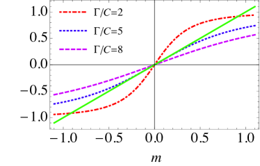
Figure 1: Saddle point equation (19) with $m=m_{i}$ at $J=1$, $\lambda=1.5$, $T/C=0.02$ with various values of $\Gamma$. For $\Gamma/C<5$ there are three intersections (ferromagnetic phase), and above $\Gamma/C=5$ there is only one, $m=0$ (paramagnetic phase).

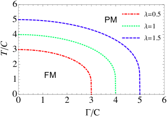
Figure 2: The critical line in the $(\Gamma/C,T/C)$ plane for $J=1$ and $\lambda=0.5$, $1.0$ and $1.5$. The ordered (disordered) phase is below (above) the lines.

IV Ferromagnetic $p$-body interactions with $q$-body penalty

Having studied the two-body case, we now move on to the generalization of NQAC to ferromagnetic systems with $p$-body interactions and $q$-body penalties. An NQAC Hamiltonian for the $p$-spin model with $q$-body penalty interactions within each logical qubit reads:

$$H= -\Gamma\sum_{i}\sum_{c_{i}}\sigma^{x}_{ic_{i}}-JN\left({1\over N}\sum_{i}\sum_{c_{i}}\sigma^{z}_{ic_{i}}\right)^{p}$$

$$-\lambda\sum_{i}\left(\sum_{c_{i}}\sigma^{z}_{ic_{i}}\right)^{q}\ .$$ (22)

The first step is to determine the free energy and scaling relations, which we do next. The $p=q=2$ case we discussed in the previous section exhibits a second-order phase transition; as we shall see the generalized models undergo a first-order phase transitions for $p\geq 3$.

IV.1 Free energy and scaling relations

By using the Suzuki-Trotter decomposition and the static ansatz, one can compute the free energy per logical qubit, to find:

$$F=(p-1)JC^{p}m^{p}+(q-1)\lambda C^{q}{1\over N}\sum_{i}m^{q}_{i}-{C\over\beta N}\sum_{i}\times$$

$$\log\left[2\cosh\beta\left((pJC^{p-1}m^{p-1}+q\lambda C^{q-1}m^{q-1}_{i})^{2}+\Gamma^{2}\right)^{1/2}\right]$$ (23)

with the same definitions of $m$ and $m_{i}$ as in Eq. (11b). The saddle-point equations are:

$$m={1\over N}\sum_{i}{Jpm^{p-1}+\lambda C^{q-p}qm^{q-1}_{i}\over\sqrt{({Jpm^{p-1}+\lambda C^{q-p}qm^{q-1}_{i})^{2}+(\Gamma/C^{p-1})^{2}}}}$$ (24)

$$\times\tanh\beta C^{p-1}\sqrt{({Jpm^{p-1}+\lambda C^{q-p}qm^{q-1}_{i})^{2}+(\Gamma/C^{p-1})^{2}}}$$ (25)

$$m_{i}={Jpm^{p-1}+\lambda C^{q-p}qm^{q-1}_{i}\over\sqrt{({Jpm^{p-1}+\lambda C^{q-p}qm^{q-1}_{i})^{2}+(\Gamma/C^{p-1})^{2}}}}$$ (26)

$$\times\tanh\beta C^{p-1}\sqrt{({Jpm^{p-1}+\lambda C^{q-p}qm^{q-1}_{i})^{2}+(\Gamma/C^{p-1})^{2}}}.$$ (27)

(28)

Each parameter scales with $C$ as

$$\lambda\to\lambda C^{q-p},\beta\to\beta C^{p-1},\Gamma\to\Gamma/C^{p-1}.$$ (29)

In the zero temperature limit, the free energy (23) reduces to the simple form

$$F = (p-1)JC^{p}m^{p}+(q-1)\lambda C^{q}{1\over N}\sum_{i}m^{q}_{i}$$

$$- {C^{p}\over N}\sum_{i}\sqrt{(pJm^{p-1}+q\lambda C^{q-p}m^{q-1}_{i})^{2}+(\Gamma/C^{p-1})^{2}}.$$

From this expression we see that the parameters appearing in the low-temperature free energy scale as:

$$\beta\to\beta,J\to JC^{p},\lambda\to\lambda C^{q},\Gamma\to\Gamma C\ ,$$ (31)

or, equivalently, using the partition function $Z=e^{-N\beta F}$:

$$\beta\to\beta C^{p},J\to J,\lambda\to\lambda C^{q-p},\Gamma\to\Gamma C^{1-p}\ .$$ (32)

The same comments as in the previous section apply regarding the difference between the saddle point and low temperature results. An interesting new aspect of the present analysis is that the effective penalty strength $\lambda$ can be affected by the nesting level if $p\neq q$. Specifically, choosing $q<p$ causes $\lambda$ to decrease with increasing nesting after rescaling, as one might expect given that this choice lowers the degree of penalty interactions relative to the logical coupling between spins.

IV.2 First-order phase transition

IV.2.1 $p=q=4$

Let us begin the analysis of phase transitions with the case $p=q=4$. The free energy simplifies to

$$F = 3C^{4}\left(Jm^{4}+\lambda{1\over N}\sum_{i}m^{4}_{i}\right)$$

$$- 2{C^{4}\over N}\sum_{i}\sqrt{(Jm^{3}+\lambda m^{3}_{i})^{2}+(\Gamma/C^{3})^{2}}.$$

Near the end of anneal, $\Gamma\sim 0$, the free energy (IV.2.1) is proportional to $C^{4}$, and thus the effective temperature decreases as $T/C^{4}$. If the temperature is very low one can expect a uniformly ordered state to be realized since the system is ferromagnetic. I.e., in this limit we expect $m=m_{i}$. The free energy at the transition point, exhibiting typical low temperature behavior ($T/C^{4}=0.01$), is plotted in Fig. 3, as a function of the magnetization $m$. The system clearly undergoes a first-order phase transition. Our numerical results show that the potential barrier at the first-order phase transition persists at any value of $\lambda$. This means that the potential barrier is not reduced by increasing $\lambda$, so that the penalty term is not helpful in this case. We can understand this as a consequence of the fact that when $p=q$, as can be seen from Eq. (IV.2.1), the effective penalty $\lambda$ simply acts to shift $J$ (i.e., $J\to J+\lambda$) if $m_{i}=m$, as we also saw in the $p=q=2$ case discussed in Sec. III.2.

We thus consider $p\neq q$, for which the role of the effective penalty $\lambda$ is different from the $p=q$ case, since then $\lambda$ cannot be absorbed into the ferromagnetic coupling $J$.

IV.2.2 $p=4$, $q=2$

The free energy at the transition point (where the free energy become degenerate) is plotted in Fig. 4 for $p=4$ and $q=2$, for various values of $\lambda$. One sees that the potential barrier becomes smaller as $\lambda$ increases, and it disappears for large values of $\lambda$.

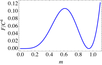
Figure 3: Free energy at the transition point normalized by $C^{4}$ as a function of $m$ for $p=q=4$. Parameters are chosen to be $J=1,\lambda=1,\Gamma/C^{3}=2.37,T/C^{4}=0.01.$

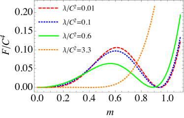
Figure 4: Free energy at the transition point, normalized by $C^{4}$, as a function of $m$, for $p=4$, $q=2$, and $J=1,T/C^{4}=0.01.$ The red dotted line is for $\lambda/C^{2}=0.01$ and $\Gamma/C^{3}=1.2$, the blue dashed line for $\lambda/C^{2}=0.1$ and $\Gamma/C^{3}=1.3$, the green solid line for $\lambda/C^{2}=0.6$ and $\Gamma/C^{3}=2.0$, and the orange dotted line for $\lambda/C^{2}=3.3$ and $\Gamma/C^{3}=6.7$.

The height ($\Delta F$) and the width ($\Delta m$) of the potential barrier at the transition point as functions of the effective penalty strength are shown in Fig. 5.

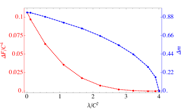
Figure 5: The height of the barrier $\Delta F$ and the width $\Delta m$ at the transition point, for the same parameters as in Fig. 4. The dotted line (red) represents $\Delta F/C^{4}$ and the dashed line (blue) represents $\Delta m$.

The system is in the paramagnetic phase for large $\Gamma\gg 1$ while it is in the ordered phase at $\Gamma=0$. Therefore, the phase transition exists for all values of $\lambda$. However, as $\lambda$ increases, the first-order phase transition in the ground state softens, in the sense of smaller values of the potential barrier height $\Delta F$ and width $\Delta m$, as seen in Fig. 5. The order of the phase transition eventually changes from first to second when the free energy barrier vanishes at $\lambda/C^{2}=4$.

In order to study the phase transition in more detail, we expand the free energy around $m=0$ to quartic order:

$$F/C^{4}\simeq\left({\lambda\over C^{2}}-{2\lambda^{2}\tanh(\beta\Gamma)\over C\Gamma}\right)m^{2}$$ (34)

$$+\left(3-{2C\beta\lambda^{4}\over\Gamma^{2}}-{8C\lambda\tanh(\beta\Gamma)\over\Gamma}+{2C\lambda^{4}\Gamma\tanh(\beta\Gamma)\over\Gamma^{4}}\right.$$ (35)

$$\left.+{2C\beta\lambda\tanh^{2}(\beta\Gamma)\over\Gamma^{2}}\right)m^{4}\ ,$$ (36)

where we omitted the constant term $F(0)/C^{4}$ and higher order terms in $m$. Let us assume that the phase transition is dominated by the quadratic and quartic terms in the expansion. The point $m=0$ becomes perturbatively unstable when the coefficient of $m^{2}$ is negative, and the critical point is at $\Gamma_{c_{2}}$ where the coefficient of the $m^{2}$ term vanishes. In the following we use the subindices $c_{1}$ and $c_{2}$ to represent critical points potentially associated with first and second order phase transitions. If the coefficient of $m^{4}$ is positive at $\Gamma=\Gamma_{c_{2}}$, $m=0$ is a global minimum for $\Gamma\geq\Gamma_{c_{2}}$. Therefore, the phase transition will be of second order. If the coefficient of $m^{4}$ is negative, then the global minimum must be at $m=m_{c}\neq 0$; $F(m=0)>F(m_{c})$ at $\Gamma=\Gamma_{c_{2}}$. This means that there must be a first order phase transition at $\Gamma_{c_{1}}>\Gamma_{c_{2}}$ where $F(m=0)=F(m_{c}\neq 0)$. In Fig. 6, we show the critical value $\lambda_{c}$, as a function of temperature, at which the order of the phase transition changes from first to second: a second order phase transition for $\lambda>\lambda_{c}$ and a first order phase transition for $\lambda<\lambda_{c}$.

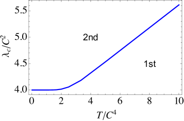
Figure 6: The critical value $\lambda_{c}$ at which the phase transition changes from first order to second order for $p=4$ and $q=2$. The region with $\lambda>\lambda_{c}$ exhibits a second order phase transition, while the region with $\lambda<\lambda_{c}$ exhibits a first order phase transition. Above $T/C^{4}\simeq 12.5$ the ferromagnetic phase disappears due to the strong thermal fluctuations.

To understand the impact of an increasing effective penalty strength $\lambda$, consider Fig. 6 at a fixed temperature $T$. Starting from small effective penalty in the first order region, increasing $\lambda$ has the effect of eventually crossing the critical line into the second order phase transition region. From the point of view of successful QA, a second order phase transition is preferred as — unlike the first order case — it does not require tunneling through the free energy barrier, an event that is exponentially suppressed in the barrier width and height. At $T=0$ a first (second) order quantum phase transition is commonly associated with gap that closes exponentially (polynomially) in system size; we corroborate this in Sec. IV.3.2 below.

Fig. 6 also shows that the higher the temperature, the larger $\lambda$ needs to be in order to affect the transition from the first order to the second order regime. Since the temperature is rescaled by $C^{4}$, increasing the nesting level makes the effective temperature smaller, which has the same beneficial effect for QA as increasing the effective penalty.

IV.3 Penalty strength and first-order phase transitions at zero temperature for $q=2$

In this subsection we consider the $T=0$ case, when all the phase transitions are quantum. We study in more detail when first order phase transitions disappear for a sufficiently strong effective penalty. We only consider the $q=2$ case.

The leading order terms of the Taylor expansions of the free energy (IV.1) with $m=m_{i}$ around the origin $m=0$ are then:

$$p=3:$$ (37a)

$${F\over C^{3}}\simeq{\lambda\over C}\left(1-{2C\lambda\over\Gamma}\right)m^{2}+2J\left(1-{3C\lambda\over\Gamma}\right)m^{3}$$

$$p=4:$$ (37b)

$${F\over C^{4}}\simeq{\lambda\over C^{2}}\left(1-{2C\lambda\over\Gamma}\right)m^{2}+\left(3J-{8JC\lambda\over\Gamma}+{2C\lambda^{4}\over\Gamma^{3}}\right)m^{4}$$

$$p\geq 5:$$ (37c)

$${F\over C^{p}}\simeq{\lambda\over C^{p-2}}\left(1-{2C\lambda\over\Gamma}\right)m^{2}+\left({2\lambda^{4}\over\Gamma^{3}}\right)m^{4}$$

We omitted the $m$-independent term $F(0)/C^{p}$ as well as higher order terms in $m$. As in Sec. IV.2, $m=0$ becomes perturbatively unstable when the coefficient of the quadratic term ($m^{2}$) becomes negative. The critical point is $\Gamma_{c2}=2C\lambda$. For $\Gamma>\Gamma_{c_{2}}$, the coefficient is positive and $m=0$ is perturbatively stable. For $\Gamma<\Gamma_{c_{2}}$, $m=0$ is perturbatively unstable.

It is important to note that this quadratic term does not exist if the effective penalty vanishes ($\lambda=0$); in this case the phase transition is always of first order. It is the quadratic penalty terms that enable the second order phase transitions. Whether the first order phase transitions persist or not depends on the higher order terms. If the coefficient of the next lowest order term beyond $m^{2}$ is positive at $\Gamma=\Gamma_{c_{2}}$, then the phase transition will be of second order, and if it is negative then the phase transition will be of first order. Of course, this estimation of the first order phase transition is based on the assumption that the lowest and the second lowest terms in the Taylor expansion determine the phase transition. As we will show in this section, this assumption is in fact not valid for higher $p$.

IV.3.1 $p=3$

Let us first consider $p=3$. From Eq. (37a), both of the coefficients of $m^{2}$ and $m^{3}$ are positive for $\Gamma\geq 3C\lambda$, so that $m=0$ is the global minimum. For $\Gamma_{c_{2}}=2C\lambda<\Gamma<3C\lambda$, the coefficient of $m^{3}$ becomes negative while that of $m^{2}$ is still positive. This suggests that there exists a critical value $\Gamma_{c_{2}}<\Gamma_{c_{1}}$ and for $\Gamma\leq\Gamma_{c_{1}}<3C\lambda$, the global minimum shifts from $m=0$ to $m=m_{c}\neq 0$. The critical value $\Gamma_{c_{1}}$ is determined by $F(0)=F(m_{c})$. This is a first order phase transition since $m=0$ and $m=m_{c}$ are separated by a potential barrier. Since $\Gamma_{c_{2}}<\Gamma_{c_{1}}$ independent of the value of $\lambda$, the first order phase transition is inevitable. We show the difference between $\Gamma_{c_{1}}$ and $\Gamma_{c_{2}}$ in Fig. 7.

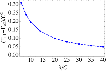
Figure 7: The $p=3$ case. The difference of the critical values of the transverse field $(\Gamma_{c_{1}}-\Gamma_{c_{2}})/C^{2}$ as a function of $\lambda/C$. Since $\Gamma_{c_{1}}>\Gamma_{c_{2}}$, there is only a first order phase transition.

IV.3.2 $p=4$

For $p=4$, the coefficient of the subleading term, namely the coefficient of $m^{4}$ in Eq. (37b) at the critical point $\Gamma_{c_{2}}=2C\lambda$ is $\lambda/C^{2}-4$. The coefficient is negative for ${\lambda/C^{2}}<4$ which means that there is only a first order phase transition at $\Gamma_{c_{2}}<\Gamma_{c_{1}}$. It is positive for ${\lambda/C^{2}}>4$ and a second order phase transition takes place to destabilize $m=0$.

While this conclusion is based on a Taylor expansion analysis, a full numerical analysis shows that there is no first order phase transition for $p=4$ above ${\lambda/C^{2}}=4$. Indeed, this is already clear from Fig. 5, which is for $T/C^{4}=0.01$; the only change at $T=0$ is that the vertical axis scale is somewhat compressed.

Figure 8 shows the free energy as a function of $m$ near the critical point $\Gamma/C^{3}=8$ for $p=4$ and $\lambda/C^{2}=4$ where the first-order phase transition disappears. One can see that the phase transition is of second order even though the interaction has a higher order power ($p>2$). The point at which $\lambda/C^{2}=4$ and $\Gamma/C^{3}=8$ is where the coefficients of the first two leading terms $m^{2}$ and $m^{4}$ vanish simultaneously, and the next order leading term ($m^{6}$) has a positive coefficient. Above this value of $\lambda$ the phase transition is always of second order, and below it is of first order.

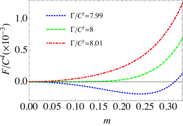
Figure 8: Free energy around the critical point for $\lambda/C^{2}=4$, $\Gamma/C^{3}=8$ for $p=4$.

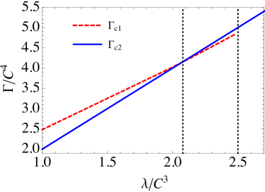
Figure 9: The critical values $\Gamma_{c_{1}}/C^{4}$ and $\Gamma_{c_{2}}/C^{4}$ as a function of $\lambda/C^{3}$ for $p=5$. For $\lambda/C^{4}<2.078$, $\Gamma_{c_{1}}>\Gamma_{c_{2}}$. Therefore, there is a first order phase transition. For $2.078<\lambda/C^{4}<2.5$ the first order phase transition and the second order phase transition coexist. For $2.5<\lambda/C^{4}$, there is only a second order phase transition.

IV.3.3 $p\geq 5$

The Taylor expansion for $p=5$, Eq. (37c), suggests that the subleading $m^{4}$ term is always positive. This does not mean that the phase transition is always of second order. In fact, since there is a single first order phase transition for $p\geq 3$ in the absence of the effective penalty, by continuity there must be a first order phase transition when $\lambda$ is very small. This suggests that higher order terms in $m$ become relevant for these first order phase transitions. In Fig. 9, we plot $\Gamma_{c_{1}}$ and $\Gamma_{c_{2}}$ as a function of the effective penalty coupling $\lambda/C^{3}$. They cross at $\lambda/C^{3}\approx 2.078$. When $\lambda/C^{3}<2.078$, there is a single first order phase transition between $m=0$ and $m=m_{c}>0$. For $2.078<\lambda/C^{3}$, $m=0$ becomes perturbatively unstable and there is a second order phase transition from $m=0$ to $m=m_{c}>0$. There are two different cases after the second order phase transition. For $2.078<\lambda/C^{3}<2.5$, there is a first order phase transition at $\Gamma_{c_{1}}<\Gamma_{c_{2}}$ and the order parameter changes discontinuously from $m_{c}$ to $m>m_{c}$. On the other hand, for $2.5<\lambda/C^{3}$ there is no phase transition other than the second order phase transition from $m=0$ to $m=m_{c}$.

This behavior is general for $p\geq 5$. In Fig. 10, we show the order of the phase transitions for various values of $p$ and $\lambda$. As we saw earlier, only the first order phase transition exists for $p=3$. For $p=4$, the first order phase transition changes into a second order phase transition at $\lambda/C^{p-2}=4$. For $p\geq 5$ there is a parameter region where the first order and the second order phase transitions coexist. The first order phase transition disappears above a certain $p$-dependent value of $\lambda/C^{p-2}$.

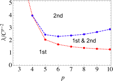
Figure 10: The order of the phase transitions for various values of $p$ and $q=2$. For $p=3$ there is a unique first order phase transition. For $p=4$, there is a critical value of $\lambda$ above which the phase transition becomes of second order. For $p\geq 5$, there is an intermediate region where the first and second phase transitions coexist. For $p\geq 4$, all the phase transitions turn into second order phase transitions for sufficiently large $\lambda$.

IV.4 Energy gap from instanton analysis

While the width and height of the free energy barrier are useful measures for a qualitative inference of the change of the energy gap Matsuura et al. (2017), one can estimate the energy gap more accurately in terms of the eigenstates of the effective Hamiltonian. The energy gap is given by the instanton solution in the Euclidean path integral which connects two different minima of the free energy. When a transition between two minima happens instantaneously, the energy gap can be approximated by the overlap of two eigenstates of the effective Hamiltonian at each local minimum Jörg et al. (2010); Matsuura et al. (2016, 2017).

Let us discuss this viewpoint in some detail. At the critical point, there are two minima characterized by the order parameters $m=m_{0}=0$ and $m=m_{c}>0$. A first-order phase transition happens between $m_{0}$ and $m_{c}$. The last term of the free energy  (23) , which represents quantum effects as it involves $\Gamma$, takes the form of $\cosh(\beta\epsilon)$ with $\epsilon=\sqrt{(pJC^{p-1}m^{p-1}+q\lambda C^{q-1}m^{q-1})^{2}+\Gamma^{2}}$ after using $m=m_{i}$. This contribution to the energy can be reproduced by the linearized Hamiltonian which is obtained by replacing every power $>1$ of the Pauli matrices $\sigma^{z}_{ic}$ by the expectation value $m$:

$$H_{\rm eff}(m)=-(pJC^{p-1}m^{p-1}+q\lambda C^{q-1}m^{q-1})\sigma^{z}-\Gamma\sigma^{x}\ .$$ (38)

Let $|m_{0}\rangle$ and $|m_{c}\rangle$ be the ground states of $H_{\rm eff}(m_{0})$ and $H_{\rm eff}(m_{c})$, respectively. Then the energy gap $\Delta$ is (for a detailed justification see Appendix B of Ref. Matsuura et al. (2017)):

$$\Delta\sim|\langle m_{0}|m_{c}\rangle|^{NC}$$ (39)

Figure 11 shows the wavefunction overlap as a function of the effective penalty $\lambda$. It reaches $1$ at the critical penalty strength $\lambda/C^{2}=4$, which implies that the gap ceases to decrease exponentially as a function of the system size. This agrees with the conclusions we drew above about the phase transition changing from first order (corresponding to an exponentially decreasing gap) for $\lambda/C^{2}<4$ to second order for $\lambda/C^{2}\geq 4$.

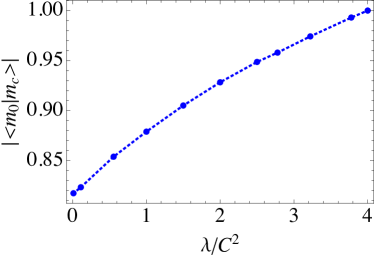
Figure 11: The overlap of the $m=m_{0}=0$ and $m=m_{\rm c}$ eigenstates of the effective $T=0$ Hamiltonian (38), as a function of the effective penalty $\lambda$ for $p=4,q=2$. This overlap determines the closing of the gap, as per Eq. (39).

IV.5 $C$ dependence and $\lambda$ dependence

As can be seen from Eq. (23), the free energy scales as $C^{\text{max}(p,q)}$ for large $C$. Since the occupancy rate of the excited states is suppressed by the factor $e^{-\beta NF(m)}$, thermal fluctuations are efficiently suppressed in terms of the nesting level $C$. This is an essential feature required for scalable error correction, and NQAC satisfies this condition. Note that the free energy in PQAC Pudenz et al. (2014, 2015); Mishra et al. (2015) scales linearly in $C$ Matsuura et al. (2016, 2017). Therefore, NQAC removes thermal noise more efficiently than PQAC.

While increasing $C$ is beneficial for suppressing thermal fluctuations, it may enhance Landau-Zener transitions at the critical point in a first order phase transition: the energy gap is suppressed by a power of $C$ [Eq. (39)]. On the other hand, the wavefunction overlap $|\langle m_{0}|m_{c}\rangle|$ in Eq. (39) can be increased by increasing the penalty coupling $\lambda$, as shown Fig. 11. Therefore, one can adjust the parameters $\{C,\lambda\}$ so that both thermal fluctuations and Landau-Zener transitions are efficiently suppressed.

V Antiferromagnetic case

In this section we study fully antiferromagnetic systems, where the coupling satisfies $J<0$. Unlike the ferromagnetic case, the long-range antiferromagnetic system is frustrated and thus exhibits different behavior.

The free energy and the saddle point equations are the same as those in the ferromagnetic case, i.e., Eq. (23), the only difference being that $J$ is replaced by $-J(<0)$. The penalty $\gamma$ coupling (and hence also the effective penalty $\lambda$) between physical qubits within a logical qubit remains ferromagnetic as it is designed to introduce resilience against bit flips in a logical qubit. It tends to induce a ferromagnetically ordered state for each logical qubit, i.e., $m_{i}\neq 0$.

Let us assume that the total number of logical qubits is even and that the effective penalty strength is large, i.e., $\gamma\gg J$, so that the logical qubits are ordered In this case, there are two possible phases in the model with antiferromagnetic interactions. The first is the paramagnetic phase, where each logical qubit has a vanishing expectation value $m_{i}=0$ and consequently the total magnetization also vanishes: $m=0$. This phase is realized when the temperature and/or the transverse field are large. The second phase is where each logical qubit is ordered, i.e., $m_{i}=\pm n$, while the total magnetization again vanishes: $m=0$. We call this a “locally ordered phase”; it appears when the effect of $\lambda$ is stronger than that of the temperature or the transverse field. In the following we analyze these phases at or near the ground state, analytically as well as numerically. In addition, there can be metastable states as in the ferromagnetic example, which we analyze in the appendix.

Since both of the phases take $m=0$, the value of $p$ does not determine the order of the phase transition, which is different from the ferromagnetic case. Instead, the order of the phase transition is controlled by $q$. All the $J$ dependence disappears from the mean field free energy [Eq. (23)] and the $p$-dependence appears only in the scaling of parameters in $C$ discussed in Sec. IV.1.

Figure 12: Free energy barrier in the antiferromagnetic case between two phases at a first-order phase transition, at $T/C=0.03$ and $3.3$, for $p=q=4$. Contrast with Fig. 5 for the ferromagnetic case.

Assuming that the total number of spins $N$ is even, the free energy (23) reduces to:

$$F = {(q-1)\over 2}\lambda C^{q}(n^{q}+(-n)^{q})+$$

$$- {C\over\beta}\log\left.\bigg{(}2\cosh\beta\sqrt{(q\lambda C^{q-1}n^{q-1})^{2}+\Gamma^{2}}\right)$$

Let us first consider the $q=2$ case. The expression for the free energy is the same as for the ferromagnetic case with two-body interactions $p=2$ [Eq. (12)], with the local (logical qubit) order parameter $n={1\over C}\langle\sum_{c}\sigma^{z}_{ic}\rangle$ replacing the global order parameter $m={1\over NC}\langle\sum_{i,c}\sigma^{z}_{ic}\rangle$ appearing in the ferromagnetic case. I.e., the free energy of the ferromagnetic system with the order parameter $m$ is the same as that of the antiferromagnetic system with the different order parameter $n$. Therefore, the latter has a second-order phase transition. It should be noted that the conventional $p$-body antiferromagnetic Ising model $(C=1)$ does not have a phase transition for $p$ even.

The phase transition point is determined in the same way as in the ferromagnetic case, where we derived Eq. (21). The critical parameter values satisfy $2\lambda C\tanh(\beta\Gamma)/\Gamma=1$, which is $p$-independent. The paramagnetic and locally ordered phases exist in the respective regions

$$2\lambda C\tanh(\beta\Gamma)/\Gamma<1\leavevmode\nobreak\ \leavevmode\nobreak\ \leavevmode\nobreak\ \ :\quad m_{i}=0$$ (41a)

$$2\lambda C\tanh(\beta\Gamma)/\Gamma>1\leavevmode\nobreak\ \leavevmode\nobreak\ \leavevmode\nobreak\ \ :\quad m_{i}\equiv\pm n\neq 0$$ (41b)

It is clear from these equations that high temperature and large transverse field favor the paramagnetic phase (all $m_{i}=0$), while large local ferromagnetic coupling $\lambda$ favors the locally ordered phase (all $m_{i}\neq 0$). In addition, we see that a larger value of $C$ also favors the locally ordered phase. This is because $C$ aligned spins behave as a single spin-$C$ vector, thus increasing the effective ferromagnetic coupling by $C^{2}$.

It is straightforward to extend the analysis to a general $q$. For even $q(\geq 4)$, the phase transition is of first order, and for odd $q(\geq 3)$ there is no phase transition since the state with the lowest value of the free energy always has $m_{i}\neq 0$.

Figure 12 shows the height of the free energy barrier at the transition point for $q=4$. Clearly, a larger value of the penalty coefficient $\lambda$ has a higher barrier height, in sharp contrast to the ferromagnetic case (Fig. 5). The $T/C$-dependence is very weak. The jump in the order parameter $\Delta m$ at the transition does not depend on $\lambda$ and $T/C$ within the numerical precision of our simulations.

VI Hybrid NQAC-PQAC strategy

The penalty term in NQAC prevents transitions from the code space by imposing ferromagnetic couplings between physical qubits within a logical qubit. This is not the only way to impose a penalty. For instance, one can introduce an independent and designated penalty qubit for each logical qubit, and connect this penalty qubit and the physical qubits in the logical qubit ferromagnetically. We refer to this method as penalty quantum annealing correction; it was proposed in Ref. Pudenz et al. (2014) and further studied in Refs. Pudenz et al. (2015); Mishra et al. (2015). As shown in Refs. Matsuura et al. (2016, 2017), phase transitions can disappear or be significantly weakened when the penalty coupling is sufficiently large.

In this section we consider a hybrid penalty-nested QAC model, and introduce designated penalty qubits into NQAC.

VI.1 Ferromagnetic case

Let us explicitly write the Hamiltonian for the case of the $p$-spin ferromagnetic model,

$$H = -{NJ}\left({1\over N}\sum_{i=1}^{N}\sum_{c_{i}=1}^{C}\sigma_{ic_{i}}^{z}\right)^{p}-\lambda\sum_{i=1}^{N}\left(\sum_{c_{i}=1}^{C}\sigma_{ic_{i}}^{z}\right)^{q}$$ (43)

$$-\Gamma\sum_{i=1}^{N}\sum_{c_{i}=1}^{C}\sigma_{ic_{i}}^{x}-\eta\sum_{i=1}^{N}\left(\sum_{c_{i}=1}^{C}\sigma_{ic_{i}}^{z}\right)\sigma^{z}_{i0}\ ,$$

where each designated penalty qubit (labeled $i0$) couples ferromagnetically via $\sigma^{z}_{i0}$ to the physical qubits within a logical qubit labeled by $i$ with a coupling strength $\eta$. The corresponding free energy is

$$F = (p-1)JC^{p}m^{p}+(q-1)\lambda{C^{q}\over N}\sum_{i}m^{q}_{i}$$ (45)

$$-{1\over\beta N}\log\left(\sum_{a_{i}=\pm}\left[\prod_{i}2\cosh\beta v^{a_{i}}_{i}\right]^{C}\right)$$

where

$$v^{\pm}_{i}=C^{p-1}\times$$ (46)

$$\sqrt{[pJm^{p-1}+q\lambda C^{q-p}m^{q-1}_{i}\pm(\eta/C^{p-1})]^{2}+(\Gamma/C^{p-1})^{2}}\ .$$

The penalty coupling is rescaled as $\eta\mapsto{\eta/C^{p-1}}$, and the effective temperature decreases as $T/C^{p}$ (from the partition function $Z=e^{-N\beta F}$), which serves to suppress thermal excitations.

Let us now focus our attention on the ground state at zero temperature. Since the system is ordered in the ground state, the local magnetization of each logical qubit assumes the same value as that of the total system, i.e., $m=m_{i}$. Then Eq. (45) yields:

$$F=(p-1)JC^{p}m^{p}+(q-1)\lambda C^{q}m^{q}-C^{p}\times$$ (47)

$$\sqrt{(pJm^{p-1}+q\lambda C^{q-p}m^{q-1}+(\eta/C^{p-1}))^{2}+(\Gamma/C^{p-1})^{2}}\ .$$

To study the stability of the paramagnetic state $m=0$, we perform a Taylor expansion of $F$ around $m=0$ [compare to Eq. (37) for the NQAC case]. For $p>q$:

$$F/C^{p}\simeq-{q(\eta\lambda)C^{q-p}\over\sqrt{\eta^{2}+\Gamma^{2}}}m^{q-1}+\mathcal{O}(m^{q})$$ (48)

where we neglected a constant term $F(0)$. For $p=q$:

$$F/C^{p}\simeq-{q(\eta(J+\lambda))\over\sqrt{\eta^{2}+\Gamma^{2}}}m^{q-1}+\mathcal{O}(m^{q})$$ (49)

If there is no nesting penalty coupling (i.e., $\lambda=0$) then:

$$F/C^{p}\simeq-{p(J\eta)\over\sqrt{\eta^{2}+\Gamma^{2}}}m^{p-1}+\mathcal{O}(m^{p})$$ (50)

In all cases, we see that the stable state is ferromagnetic, $m\neq 0$.

Figure 13 shows the critical line for $T=0,p=4$ and $q=2$. In the parameter region ($\eta,\lambda$) below the line the system undergoes a first order phase transition, while above the line it undergoes a second order phase transition. The critical value of $\lambda$ decreases rapidly when $\eta$ is turned on and then decreases almost linearly above $\eta/C^{3}\sim 0.1$. As expected, the critical value of $\eta/C^{3}$ at $\lambda/C^{2}=0$ reproduces the result for penalty quantum annealing correction found in Ref. Matsuura et al. (2016). The main point is that the two types of penalties are complementary, in the sense that increasing one (say $\eta$) allows for a smaller value of the other (say $\lambda$).

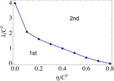
Figure 13: Critical values of the penalty strength $\eta/C^{3}$ and $\lambda/C^{2}$ for $T=0,p=4,q=2,J=1$, for the hybrid NQAC-PQAC strategy and ferromagnetic coupling. The phase transition is of first order below the blue dotted line and of second order above it. Since the second order phase transition region is preferred, increasing $\eta$ in the hybrid NQAC-PQAC strategy allows for a lower value of $\lambda$ than in the pure NQAC case.

VI.2 Antiferromagnetic case

Assuming $\gamma\gg J$ as in Sec. V to ensure ordering of the logical qubits, the ground state of the antiferromagnetic system has $m_{i}=\pm n$, $m=0$. The free energy is

$$F = (q-1)\lambda C^{q}n^{q}-{1\over\beta N}$$ (53)

$$\log\left(\left[2\cosh\beta\sqrt{(q\lambda C^{q-1}n^{q-1}+\eta)^{2}+\Gamma^{2}}\right]^{C}\right.$$

$$\left.+\left[2\cosh\beta\sqrt{(q\lambda C^{q-1}n^{q-1}-\eta)^{2}+\Gamma^{2}}\right]^{C}\right)^{N}\ .$$

At zero temperature this becomes:

$$F = (q-1)\lambda C^{q}n^{q}-$$ (55)

$$\leavevmode\nobreak\ -\sqrt{(q\lambda C^{q}|n|^{q-1}+C\eta)^{2}+(C\Gamma)^{2}}$$

The free energy in this case is identical to the free energy of the ferromagnetic system with a designated penalty term discussed in Refs. Matsuura et al. (2016, 2017), after the rescaling $\eta\mapsto C\eta$, $\Gamma\mapsto C\Gamma$. This system has a rather remarkable feature. When $\eta=0$, there is, respectively, a second and a first order phase transition for $q=2$ and $q\geq 3$. At finite $\eta$, the second order phase transition for $q=2$ disappears at $T=0$. For $q\geq 3$ and $T=0$, there is a first order phase transition for $\eta$ below a critical value $\eta_{c}$. However, the strength of the first order phase transition becomes weaker as $\eta$ increases and above the critical value $\eta_{c}$, the first order phase transition disappears. At finite temperature, the first order phase transition exists at any value of $\eta$. However, the strength of the phase transition significantly weakens as $\eta$ increases. More details can be found in Refs. Matsuura et al. (2016, 2017).

To summarize, the penalty coupling $\lambda$ and the nesting level $C$ reduce or effectively remove the thermal fluctuations. While the energy gap closing associated with increased nesting level $C$ (recall Sec. IV.5) still exists in NQAC, it can be removed or significantly weakened by introducing designated penalty qubits and their coupling $\eta$, as illustrated in Fig. 13.

VII Discussion and Conclusions

We have studied nested quantum annealing correction (NQAC) Vinci et al. (2016); Vinci and Lidar (2017) and the combination of NQAC and penalty quantum annealing correction (PQAC) Pudenz et al. (2014, 2015) at zero and finite temperatures. While PQAC (studied theoretically in Refs. Matsuura et al. (2016, 2017)) has designated penalty qubits which serve to induce a symmetry breaking field, NQAC does not have designated penalty qubits and therefore the penalty coupling itself does not induce symmetry breaking. Nevertheless, we have shown that first-order phase transitions can be removed or significantly weakened when the interaction strength between physical qubits within a logical qubit is chosen appropriately. Moreover, the nested structure works to efficiently reduce thermal fluctuations: for $p$-body coupling, the temperature $T$ is reduced effectively to $T/C^{p}$. Therefore, NQAC helps to stabilize the ground state by reducing thermal fluctuations, and serves as a means to address the ‘temperature scaling law’ problem identified in Ref. Albash et al. (2017), that in order to serve as optimizers, quantum annealer temperatures must be appropriately scaled down with problem size.

While a larger value of the penalty coefficient is beneficial for keeping the state in the ground state, it may cause a different problem. A larger value of the penalty term creates local minima in the free energy for excited states, as detailed in the Appendix. Once the system state becomes excited and trapped by one of those metastable states, it may be difficult to escape to the ground state if the penalty coupling is too strong. This is a difficult problem to analyze, and we leave the evaluation of transitions between metastable states and the ground state for future investigations.

The success of NQAC sheds some light on the computational efficiency and the local structure of the problem. In PQAC, the order parameters are the expectation values of total spins Matsuura et al. (2016, 2017). On the other hand, NQAC has an extensive number of order parameters ($m_{i}$) in addition to the expectation value of the total spin ($m$). When the penalty coupling is strong, the behavior of the free energy is determined by the local order parameters $m_{i}$. Therefore, by tuning the local physics (the strength of the penalty coupling $\gamma$), one can change the structure of the phase transition of the whole system. In our examples, even when the original problem has a first-order phase transition, e.g., for the case of $p\geq 3$, by encoding qubits properly in NQAC with $q=2$, one can change the order of the phase transition into second. It is an interesting problem how these results generalize beyond simple mean-field models with uniform interactions.

VIII acknowledgement

The work of WV and DL was (partially) supported under ARO grant number W911NF-12-1-0523, ARO MURI Grant Nos. W911NF-11-1-0268 and W911NF-15-1-0582, and NSF grant number INSPIRE-1551064. This research is based upon work partially supported by the Office of the Director of National Intelligence (ODNI), Intelligence Advanced Research Projects Activity (IARPA), via the U.S. Army Research Office contract W911NF-17-C-0050. The views and conclusions contained herein are those of the authors and should not be interpreted as necessarily representing the official policies or endorsements, either expressed or implied, of the ODNI, IARPA, or the U.S. Government. The U.S. Government is authorized to reproduce and distribute reprints for Governmental purposes notwithstanding any copyright annotation thereon.

Appendix A Derivation

In this Appendix, we derive the free energy of NQAC by using mean field theory. We consider an NQAC Hamiltonian

$$H=H_{X}+H_{Z}$$ (56)

where, as in Eq. (IV):

$$H_{Z} \equiv-{JN}\left({1\over N}\sum_{i=1}^{N}\sum_{c_{i}=1}^{C}\sigma_{ic_{i}}^{z}\right)^{p}-\lambda\sum_{i=1}^{N}\left(\sum_{c_{i}=1}^{C}\sigma_{ic_{i}}^{z}\right)^{q}$$ (57a)

$$H_{X} \equiv-\Gamma\sum_{i=1}^{N}\sum_{c_{i}=1}^{C}\sigma_{ic_{i}}^{x}\ .$$ (57b)

From now on we replace the double subscript $ic_{i}$ by $ia$ to simplify the notation, and keep in mind that $a$ enumerates the physical qubits within the $i$-th logical qubit.

Skipping many steps which parallel the calculation in Appendix A of Ref. Matsuura et al. (2017), the partition function $Z=\text{tr}(e^{-\beta H})$ is computed via the Suzuki-Trotter decomposition:

$$Z = \lim_{M\to\infty}\text{tr}\left(e^{-{\beta\over M}H_{X}}e^{-{\beta\over M}H_{X}}\right)^{M}$$ (58)

$$= \lim_{M\to\infty}\prod_{i}^{N}\prod_{\alpha}^{M}\int dm_{\alpha}d\tilde{m}_{\alpha}dm_{i\alpha}d\tilde{m}_{i\alpha}\exp\left[i\tilde{m}_{\alpha}\left(NCm_{\alpha}-\sum_{i=1}^{N}\sum_{a=1}^{C}\sigma_{ia}^{z}(\alpha)\right)+{\beta J\over M}NC^{p}m_{\alpha}^{p}\right.+$$ (59)

$$+ \left.\sum_{i}\left(i\tilde{m}_{i\alpha}\left(Cm_{i\alpha}-\sum_{a=1}^{C}\sigma_{ia}^{z}(\alpha)\right)+{\beta\lambda\over M}C^{q}m_{i\alpha}^{q}\right)+{\beta\Gamma\over M}\sum_{i=1}^{N}\sum_{a=1}^{C}\sigma_{ia}^{x}(\alpha)\right]\prod\langle\sigma|\sigma\rangle\,,$$ (60)

where $M$ is the Trotter number and

$$\prod\langle\sigma|\sigma\rangle\equiv\prod_{c=1}^{C}\langle\sigma^{z}_{ic}(\alpha)|\sigma^{x}_{ic}(\alpha)\rangle\langle\sigma^{x}_{ic}(\alpha)|\sigma^{z}_{ic}(\alpha+1)\rangle.$$ (61)

We use the static ansatz where all the variables are Trotter index $\alpha$ independent; $m_{\alpha}=m,\tilde{m}_{\alpha}=\tilde{m},m_{i\alpha}=m_{i},\tilde{m}_{i\alpha}=\tilde{m}_{i}$. We also rescale $(\tilde{m},\tilde{m}_{i})$ to ${1\over M}(\tilde{m},\tilde{m}_{i})$. Then, in the thermodynamic limit $N\to\infty$,

$$Z = \exp\left(iNC\tilde{m}m+{\beta JN}C^{p}m^{p}+iC\sum_{i}\tilde{m}_{i}m_{i}+C^{q}\sum_{i}{\beta\lambda}m_{i}^{q}\right)\left(\mathop{\mathrm{Tr}}\exp\left(-\sum_{i=1}^{N}i\tilde{m}\sigma_{ia}^{z}-i\tilde{m}_{i}\sigma_{ia}^{z}+\beta\Gamma\sigma_{ia}^{x}\right)\right)^{C}$$ (62)

$$= \exp\left(iNC\tilde{m}m+{\beta JN}C^{p}m^{p}+iC\sum_{i}\tilde{m}_{i}m_{i}+C^{q}\sum_{i}{\beta\lambda}m_{i}^{q}\right)\left(\prod_{i}(e^{\sqrt{(-i\tilde{m}-i\tilde{m}_{i})^{2}+(\beta\Gamma)^{2}}}+e^{-\sqrt{(-i\tilde{m}-i\tilde{m}_{i})^{2}+(\beta\Gamma)^{2}}})\right)^{C}$$ (63)

The saddle point equations for $m$ and $m_{i}$ are

$$i\tilde{m}+\beta pJC^{p-1}m^{p-1}=0\ ,$$ (65a)

$$i\tilde{m}_{i}+\beta q\lambda C^{q-1}m^{q-1}_{i}=0\ .$$ (65b)

Inserting these into the partition function, we obtain

$$Z = \exp\left(-\beta(p-1)JNC^{p}m^{p}-\beta(q-1)\lambda C^{q}\sum_{i}m^{q}_{i}\right)$$ (66)

$$\times \left(\prod_{i}(e^{\beta\sqrt{(pJC^{p-1}m^{p-1}+q\lambda C^{q-1}m_{i}^{q-1})^{2}+\Gamma^{2}}}+e^{-\beta\sqrt{(pJC^{p-1}m^{p-1}+q\lambda C^{q-1}m_{i}^{q-1})^{2}+\Gamma^{2}}})\right)^{C}\ .$$ (67)

The free energy $F$ defined by $Z=\exp(-\beta NF)$ is

$$F = (p-1)JC^{p}m^{p}+(q-1)\lambda C^{q}{1\over N}\sum_{i}m^{q}_{i}$$ (68)

$$- {C\over\beta N}\log\left[\prod_{i}\left(e^{\beta\sqrt{(pJC^{p-1}m+q\lambda C^{q-1}m_{i})^{2}+\Gamma^{2}}}+e^{-\beta\sqrt{(pJC^{p-1}m+q\lambda C^{q-1}m_{i})^{2}+\Gamma^{2}}}\right)\right]\ .$$ (69)

Appendix B Excited states

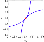
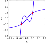
Figure 14: Solutions to Eqs. (70a) and  (70b) for $k/N=0.09,J=1,T/C=0,\gamma=0.9$. Red dots are local and global minima. (a) $\Gamma/C=3.8$; (b) $\Gamma/C=3.3$; (c) $\Gamma/C=0.07$; (d) $\Gamma/C=0$.

In the main text we analyzed ground state phase transitions, where the main focus was the energy gap between the ground and first excited states. We demonstrated that this gap becomes larger at the phase transition as the penalty strength increases. When this is the case it is more likely for the system to stay in the ground state, and errors are suppressed. However, in an open system, thermal fluctuations can cause transitions to excited states even when there is no phase transition. Therefore it is important to understand how easily excited states can relax into the ground state. The aim of this section is to understand the energy landscape of NQAC in the presence of a strong penalty coupling.

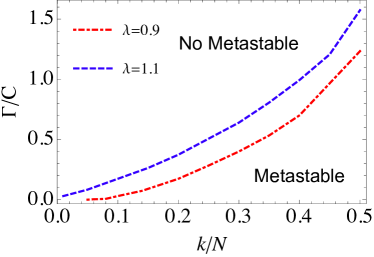
Figure 15: Phase diagrams in the $k$-$\Gamma$ plane and $k$-$T$ planes. (a): $k/N$ vs $\Gamma/C$ at $T=0$. for $\gamma=0.9$ and $\gamma=1.1$, the phase transition line is determined only by the ratio $k/N$: $k/N=0.05$ is the lowest excited state which can have a metastable state for $\gamma=0.9$. (b) $k/N$ vs $T/C$ at $\Gamma=0$. for $\gamma=0.9$ and $\gamma=1.1$. the phase transition line is determined only by the ratio $k/N$. $T/C=1.28$ is the highest temperature which can have a metastable state for $\gamma=0.9$. Above this, metastable state disappears.

B.1 The ferromagnetic case for $p=2$

Let us first consider the ferromagnetic case with $p=q=2$. In the ground state, all the spins take the same expectation value $m_{i}\equiv w_{1}$. The excited states include spin flips within a logical qubit. If the number of spin flips is less than $C/2$, we obtain a correct answer by majority vote at the end of annealing. For simplicity, we do not consider spin flips within a logical qubit and assume that all the encoded qubits in a logical qubit point in the same direction (this would be the case when the penalty coupling is large). In the following, we study when they become metastable states (local minima of the free energy).

Without loss of generality, we can assume that $w_{1}$ is positive and $w_{2}$ is negative. Substituting this into Eq. (19), the excited state is determined by:

$$w_{1} ={(2Jm+2\lambda w_{1})\over\sqrt{(2Jm+2\lambda w_{1})^{2}+(\Gamma/C)^{2}}}\times$$

$$\tanh(\beta C\sqrt{(2Jm+2\lambda w_{1})^{2}+(\Gamma/C)^{2}}),$$ (70a)

$$w_{2} ={(2Jm+2\lambda w_{2})\over\sqrt{(2Jm+2\lambda w_{2})^{2}+(\Gamma/C)^{2}}}\times$$

$$\tanh(\beta C\sqrt{(2Jm+2\lambda w_{2})^{2}+(\Gamma/C)^{2}})$$ (70b)

where

$$m={(N-k)w_{1}+kw_{2}\over N}.$$ (71)

The solutions of these equations are shown in Fig. 14. The two curves show the individual solutions of Eqs. (70a) and  (70b), and the intersections are the solutions that satisfy both equations. The red dots in Fig. 14 are local and global minima. When quantum fluctuations are large the only local minimum is the ground state [Fig. 14]. Each logical spin is in the paramagnetic state $m_{i}=0$. As the fluctuations decrease, there is a second order phase transition and the local minima are in the ferromagnetic states $m_{i}\neq 0$ [Fig. 14]. The value of each logical spin approaches $\pm 1$ [Fig. 14] and when the fluctuations become very small, the excited states start to appear as local minima in the mean field free energy [Fig. 14].

In the low temperature limit, Eqs. (70) become

$$w_{1} ={(2Jm+2\lambda w_{1})\over\sqrt{(2Jm+2\lambda w_{1})^{2}+(\Gamma/C)^{2}}}$$ (72a)

$$w_{2} ={(2Jm+2\lambda w_{2})\over\sqrt{(2Jm+2\lambda w_{2})^{2}+(\Gamma/C)^{2}}}\ .$$ (72b)

The necessary condition for the existence of metastable states is that $(w_{1},w_{2})=(\pm 1,\mp 1)$ is the solution of Eqs. (72) at $\Gamma=0$. In this limit, Eqs. (72) become $\text{sgn}(w_{1,2})=\mathop{\mathrm{sgn}}((2Jm+2\lambda w_{1,2}))$. Then $(w_{1},w_{2})=(\pm 1,\mp 1)$ can be a solution if

$$2J-{4Jk\over N}-2\lambda<0$$ (73)

This condition is satisfied for any value of $(k,N)$ if $J<\lambda$. If $J>\lambda$, it is satisfied only if the middle term ${4Jk\over N}$ compensates for the difference between $J$ and $\lambda$. Specifically, the metastable state disappears for small $k$ more easily than for large $k$. And for any $k$, the metastable state disappears as $N$ increases.

From this observation, we know that there can exist metastable states when the quantum fluctuations are small. In Fig. 15 we show the transition lines in the $(k/N,\Gamma/C)$ plane below which there exist metastable states and above which there are no metastable states. This is likewise the case for thermal fluctuations; in Fig. 15, we show the line between the existence and non-existence of metastable states in the $(k/N,T/C)$ plane Remarkably, Fig. 15 and Fig. 15 are indistinguishable, suggesting that the excited states are similarly affected by quantum and thermal fluctuations in this case.

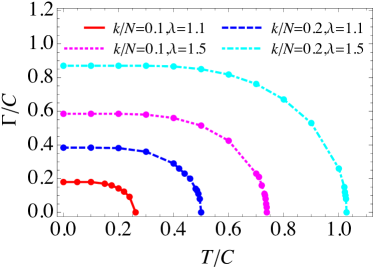
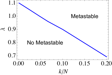
Figure 16: (a) Disappearance of lower excited states for $k/N=0.1,0.2$ in the ferromagnetic case for two values of $\lambda$: metastable states exist only below the transition lines (toward the bottom left). (b) Critical $\lambda$ as a function of $k/N$ in the ferromagnetic case. The metastable states are first excited states. Here $T/C=0.03$, $\Gamma/C=0.03$, and $J=1$.

Fig. 16 shows the transition line between the existence and the absence of metastable excited states in the $(T/C,\Gamma/C)$ plane, for various values of $k/N$ and $\lambda$. Fig. 16 shows the transition line between the existence and the absence of metastable excited states in the $(k/N,\lambda)$ plane. For a fixed penalty, when only a small number of spins inside a logical qubit have flipped there are no metastable states. But a state with many flipped spins (at fixed penalty) can be metastable. The higher the penalty, the smaller the range of no metastability, since in the limit of large penalty the only stable states are the all-up and all-down states (logical spins must be completely ordered). This explains the negative slope in Fig. 16.

B.2 Energy and degeneracy for $p=2$ in the ferromagnetic case

The existence of metastable states can affect the success probability of quantum annealing due to thermal and quantum fluctuations. At the end of annealing ($\Gamma=0$), after substituting Eqs. (72) into $H_{Z}$ [Eq. (57a)], the energy levels are:

$$E_{k} \simeq C^{2}\Big{[}J\left({N-k\over N}w_{1}+{k\over N}w_{2}\right)^{2}$$

$$+{\lambda}\left({N-k\over N}w_{1}^{2}+{k\over N}w_{2}^{2}\right)$$

$$-{N-k\over N}\sum_{i=1}^{N}2\left|J\left({N-k\over N}w_{1}+{k\over N}w_{2}\right)+\lambda w_{1}\right|$$

$$-{k\over N}\sum_{i=1}^{N}2\left|J\left({N-k\over N}w_{1}+{k\over N}w_{2}\right)+\lambda w_{2}\right|\Big{]}\ .$$ (74)

In thermal equilibrium, the probability $P_{k}$ of finding a state at $E_{k}$ is

$$P_{k}\sim d_{k}e^{-\beta E_{k}}\ ,$$ (75)

where $d_{k}$ is the degeneracy. In our case $d_{k}=2{N\choose k}$. For large $N$ and small $k$ we have $d_{k}\simeq{(n/k-1/2)^{k}e^{k}\over\sqrt{\pi k/2}}$. Note that the degeneracy increases rapidly as the energy increases. Without this entropy effect, the excited states are suppressed by the Boltzmann factor. However, the rapid increase of $d_{k}$ for excited states might change this situation and therefore change the phase transition and the annealing success probability. To analyze this, let us use Eq. (68) to define an effective action $F_{k}$ as the free energy of the $k$-th excited states:

$$F_{k}=JC^{2}m^{2}+{\lambda C^{2}\over N}((N-k)w_{1}^{2}+kw_{2}^{2})$$

$$-{C\over\beta N}\left((N-k)\log\left[2\cosh\left(\beta\sqrt{4C^{2}(Jm+\lambda w_{1})^{2}+\Gamma^{2}}\right)\right]\right.$$ (76)

$$\left.+k\log\left[2\cosh\left(\beta\sqrt{4C^{2}(Jm+\lambda w_{2})^{2}+\Gamma^{2}}\right)\right]\right)$$

$$-{1\over\beta N}\log\left[2{N\choose k}\right],$$ (77)

which takes into account the entropy (degeneracy) through the last term. The partition function is given by $Z=\sum_{k}e^{-\beta NF_{k}}$.

Figure 17: (a) $w_{1}$ and $w_{2}$ for the ground state $k/N=0$, $k/N=0.03$ and highly excited state $k/N=0.48$, as a function of $\Gamma/C$ at $T/C=0.03$, $\lambda=1$. (b) $F_{k}$ for $\Gamma/C=0.03$. The solid purple line represents the ground state free energy contribution $F_{0}/C^{2}$.

By solving Eq. (72), we plot in Fig. 17 the values of $w_{1}$ and $w_{2}$ for the ground state $k=0$, a slightly excited state $k/N=0.03$, and a highly excited state $k/N=0.48$ at $T/C=0.03$. The metastable state $w_{2}\simeq-1$ disappears quickly when $\Gamma/C$ increases from zero to finite value and the only true ground state $w_{1}=w_{2}\simeq 1$ exists. For highly excited states, $w_{1}>0$ and $w_{2}<0$ approach each other as $\Gamma/C$ increases (the blue dashed and the purple dot-dashed lines) until $\Gamma/C\sim 1.25$ and then the metastable states disappear above this value. In Fig. 17, we plot the free energy contribution from excited states at different temperatures. Because of the absence of the metastable states for smaller $k/N$, the free energy contribution of the excited states starts from a critical value of $k/N$ for a given temperature. The degeneracy contribution to Eq. (77) is $-{1\over\beta N}\log\left[2{N\choose k}\right]$. There is a unique ground state for $k=0$, for which this term vanishes. The largest degeneracy is realized at $k=N/2$. For $k=aN\gg 1,(a\in(0,1/2])$, this term scales as $T\left[a\log a+(1-a)\log(1-a)\right]$. Figure 17 shows that although the number of degenerate states increases exponentially, the contribution from the higher excited states is still subdominant as long as the effective temperature $T/C$ is low. Since this term does not depend on $C$, its effect in the normalized free energy $F_{k}/C^{2}$ is diminished as $C$ increases. This is another benefit of using NQAC.

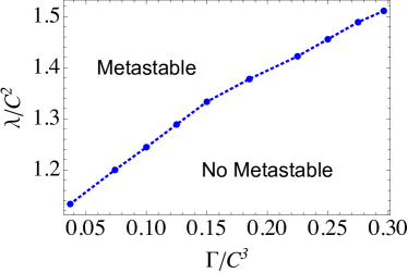
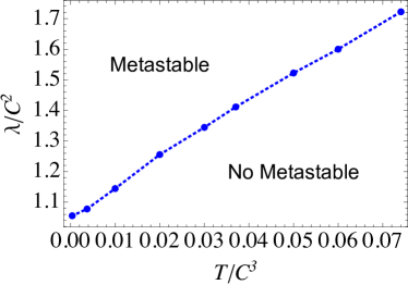
Figure 18: (a) The borders between the existence and the absence of the metastable states for $k/N=0.1$ and $p=4$. (b) Penalty coupling $\lambda/C^{2}$ as a function of temperature $T/C^{3}$ for $\Gamma=0$ and a function of $\Gamma$ for $T/C^{3}=4\times 10^{4}$ and $p=4$.

B.3 Excited states and first order phase transitions when $p\geq 3$ in the ferromagnetic case

We can extend the $p=2$ analysis to $p\geq 3$. Figure 18 shows the borders between the existence and absence of the metastable states for $p=4$. The qualitative features are the same as in the $p=2$ case: metastable states do not survive at high temperature and/or quantum fluctuations. Fig. 19 shows the potential barrier between local minima for various values of the penalty coupling. The potential barrier becomes higher as the penalty coupling increases.

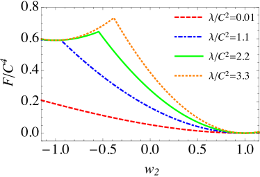
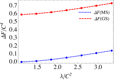
Figure 19: (a) Normalized free energy $F(w_{1}=1,w_{2})-F(w_{1}=1,w_{2}=1)$, for $k/N=0.1$, $T/C^{3}=3.7\times 10^{-4}$, $\Gamma=0.1$. The potential barrier between the metastable state $(w_{1},w_{2})\simeq(-1,1)$ and the true ground state $(w_{1},w_{2})=(1,1)$ becomes larger as $\lambda/C^{2}$ increases. (b) The free energy difference $\Delta F(MS)=F(1,w_{2}^{max})-F(1,-1)$, $\Delta F(GS)=F(1,w_{2}^{max})-F(1,1)$ between the local maximum $(w_{2}=w_{2}^{max})$, and the local minimum $(w_{2}=-1)$ or the ground state $(w_{2}=1)$ for $w_{1}=1$ seen in Fig. 19 (normalized by $C^{4}$). Other parameters: $k/N=0.1$ $T/C^{3}=3.7\times 10^{-4}$, $\Gamma/C^{3}=3.7\times 10^{-3}$.

As one can see in Fig. 19, the local free energy minimum is realized at $w_{2}\simeq-1$ while the local maximum is realized at $-1<w_{2}<0$. On the other hand, the difference between the free energy minima at $w_{2}\simeq-1$ and $w_{2}\simeq 1$ does not change as the penalty $\lambda$ changes.

To evaluate the height of the potential barrier, in Fig. 19 we plot the free energy difference between the local maximum and the local minimum, as well as the local maximum and the ground state seen in Fig. 19. It shows that increasing the penalty $\lambda$ prevents the ground state to transit into the metastable state.

Appendix C Excited states in the antiferromagnetic $p=2$ case

For simplicity let us assume that $N$ is an even number. Classically, the ground state of an antiferromagnetic system then has half of the spins pointing in the positive $z$ direction and the rest of the spins pointing in the negative $z$ direction: the ground state has $N/2$ spins with $m_{i}=1$ and $N/2$ spins with $m_{i}=-1$, and the average is $m=0$. The $k$-th excited states have $N/2\pm k$ spins with $m_{i}=1$ and $N/2\mp k$ spins with $m_{i}=-1$. The average is $m=\pm{2k\over N}$. When quantum and thermal fluctuations are induced ($\Gamma,T\neq 0$), the values of $m_{i}$ change. We study the existence and stability of excited states using a mean field analysis.

Consider the $k$-th level excited states in which ${N/2}-k$ of the $m_{i}$ are positive and ${N/2}+k$ of the $m_{i}$ are negative (since the system has $Z_{2}$ spin-flip symmetry we can make this choice without loss of generality). Similarly to Eq. (70), to determine the excited states we need to consider the following set of equations:

$$w_{1} ={(-2Jm+2\lambda w_{1})\over\sqrt{(-2Jm+2\lambda w_{1})^{2}+(\Gamma/C)^{2}}}\times$$

$$\tanh(\beta C\sqrt{(-2Jm+2\lambda w_{1})^{2}+(\Gamma/C)^{2}})$$ (78a)

$$w_{2} ={(-2Jm+2\lambda w_{2})\over\sqrt{(-2Jm+2\lambda w_{2})^{2}+(\Gamma/C)^{2}}}\times$$

$$\tanh(\beta C\sqrt{(-2Jm+2\lambda w_{2})^{2}+(\Gamma/C)^{2}})$$ (78b)

$$w_{3} ={(-2Jm+2\lambda w_{3})\over\sqrt{(-2Jm+2\lambda w_{3})^{2}+(\Gamma/C)^{2}}}\times$$

$$\tanh(\beta C\sqrt{(-2Jm+2\lambda w_{3})^{2}+(\Gamma/C)^{2}})\ ,$$ (78c)

where

$$m={({N\over 2}-k-1)w_{1}+({N\over 2}+k)w_{2}+w_{3}\over N}\ .$$ (79)

Here $({N/2}-k-1)$ of the $m_{i}$ take a value $w_{1}>0$, $({N/2}+k)$ take a value $w_{2}<0$, and a single spin takes a value $w_{3}$, which can be positive or negative. If $w_{3}$ is positive, then it is the $k$-th excited state and if it is negative, then it is the $(k+1)$-th excited state. The reason why $w_{3}$ is needed is the following, and stems from the the difference between the ferromagnetic and antiferromagnetic cases. In the ferromagnetic case, we considered the transition between the $k$-th excited state and the ground state. The $k$-th excited state has $N-k$ spins taking a positive value $w_{1}>0$ and $k$ spins taking a negative value $w_{2}<0$, while the ground state has all spins taking a positive value. The reason we consider this transition is that lower energy states, for instance the $(k-1)$-th excited state, are less stable than higher energy states against the quantum and thermal fluctuations. This feature can be seen in Fig. 16 as well as Fig. 17. Therefore, when the $k$-th excited state loses its metastability, the $(k-1)$-th excited state has already lost its meta-stability, and the transition happens collectively with all $k$ spins flipping from negative to positive. This kind of behavior is captured by two parameters $w_{1}$ and $w_{2}$. On the other hand, in the antiferromagnetic case, the lower excited states are more stable; when the $k$-th excited state loses its metastability, all the lower energy states are still metastable. Therefore, the transition from the $k$-th excited state to the $(k-1)$-th excited state happens most likely by flipping a single spin. This transition requires three parameters $w_{1,2,3}$; two of them ($w_{1}$ and $w_{2}$) do not change their signs before and after the transition, and one of them ($w_{3}$) describes the single spin that flips under the transition.

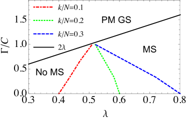
(a)  $T/C=0$

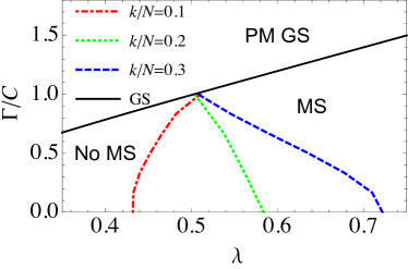
(b)  $T/C=0.33$

Figure 20: Existence of metastable excited states in the antiferromagnetic case. Panel (a): $T/C=0$; panel (b): $T/C=0.33$. Red dot-dashed, green dotted, and blue dashed lines represent $k/N=0.1,0.2$ ,and $0.3$, respectively. To the right of these lines the corresponding excited states exist as metastable states (MS), while to the left the corresponding excited states do not exist as metastable states (No MS). Above the black solid line, only the paramagnetic ground state (PM GS) exists and the free energy does not have a local minimum.

At $T=0$ and $\Gamma=0,$ the saddle point equations are

$$w_{1} = \text{sgn}(-2Jm+2\lambda w_{1})$$ (80)

$$w_{2} = \text{sgn}(-2Jm+2\lambda w_{2})$$ (81)

$$w_{3} = \text{sgn}(-2Jm+2\lambda w_{3})$$ (82)

In this case, $w_{i}$ can only be $\pm 1$. Let us assume $w_{1}=1$ and $w_{2}=-1$. For $k>0$, $w_{3}=+1$ has a lower energy and $w_{3}=-1$ has a higher energy. In order to have $w_{1}=1$, $w_{2}=-1$, $w_{3}=1$ as the solution of Eq. (82), the couplings must satisfy

$$\lambda>{2kJ\over N}$$ (83)

while for $w_{1}=1$, $w_{2}=-1$, $w_{3}=-1$, we need

$$\lambda>{2(k+1)J\over N}$$ (84)

As can be seen from Eq. (83), the ground state $k=0$ always satisfies the existence condition. Higher energy states $(k\neq 0)$ do not exist unless the penalty coupling $\lambda$ is large enough.

At finite temperature and finite transverse field ($T\neq 0,\Gamma\neq 0$), we solve the saddle point equations (78) numerically for various values of the transverse field $\Gamma$ and the penalty $\lambda$. The dashed lines in Fig. 20 separate the different phases. The excited states corresponding to each value of $k/N$ exist as metastable states of the free energy in the larger $\lambda$ region of the transition lines, while there are no corresponding metastable states in the smaller $\lambda$ region. The solid line represents a phase transition line in the ground state. The ground state is locally paramagnetic ($m_{i}=0$) above the line, and $m_{i}\neq 0$ below the line. For small excitations $k/N\ll 1$ (red dotted lines in Fig. 20) the critical $\Gamma$ increases as $\lambda$ increases, while for larger $k/N$ (green and blue dotted lines in Fig. 20) the critical $\Gamma$ decreases. This means that for a given penalty coupling $\lambda$, the metastable states of higher energy states disappear at larger values of $\Gamma$. Therefore, they are less stable. This result is the opposite of the ferromagnetic case, where higher excited states are locally more stable than lower excited states.

Figure 21: Phase diagram in the $T$-$\Gamma$ plane between the phases with $m=0$ and $m\neq 0$, for $\lambda=1.5$ and $\lambda=1$.

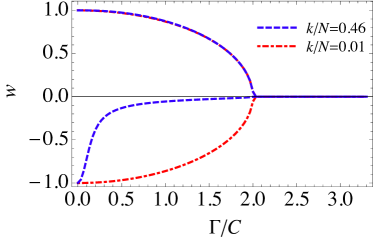
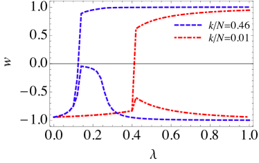
Figure 22: $w_{1}$ (starts from $1$ at $\Lambda=0$) and $w_{2}$ (starts from $-1$ at $\Lambda=0$) for a low energy state $k/N=0.01$ and highly excited state $k/N=0.46$. Here $T/C=0.03$, $\lambda=1$ (b) $w_{1}$ (ends at $1$ at $\gamma=1.0$) and $w_{2}$ (ends at $-1$ at $\gamma=1.0$) for $\Gamma/C=0.67$ and $T/C=0.03$.

Fig. 21 shows the phase transition lines in the ($T/C,\Gamma/C$) plane for the penalty coupling values $\lambda=1,1.5$. The phase transition for the ground state between the local paramagnetic $m_{i}\neq 0$ and ferromagnetic states $m_{i}\neq 0$ are given by Eq. (41b). The green dotted line is for the excited states $k/N=0.4$. One can see that the phase transition lines are fairly insensitive to the excitation level $k/N$.

In the ferromagnetic case, there are two degenerate ground states for locally ordered phase $m_{i}=\pm n$. In the antiferromagnetic case, there is an ${N\choose N/2}$-fold degeneracy in the ground state for even $N$ and an ${N\choose(N-1)/2}$-fold degeneracy for odd $N$. This is in contrast to the case of the one-dimensional Ising model with nearest-neighbor coupling $H=\pm\sum_{i}\sigma^{z}_{i}\sigma^{z}_{i+1}$. In this case, there are two ground states for both ferromagnetic and antiferromagnetic interactions. In the nested configuration, all spins are coupled. Therefore, any configurations which have the same number of positive $m_{i}$ and negative $m_{i}$ have the same energy. This fact may change the thermal behavior of the ferromagnetic and the antiferromagnetic cases. In the case of the ferromagnetic model, the number of excited states (metastable states) increases rapidly and therefore their contributions to the partition function and the transition rates between potential wells are important. On the other hand, in the antiferromagnetic case, the largest degeneracy happens in the lowest energy states and the degeneracy of the excited states is smaller.

We study the state in which $({N/2}-k)$ spins take values $m_{i}=w_{1}$, and $({N/2}+k)$ spins take values $m_{i}=w_{2}$. The ground state is $k=0$.

In Fig. 22, we show $w_{1}$ and $w_{2}$ for the low energy state $k/N=0.01$ and a highly excited state $k/N=0.46$ for $T/C=0.03$. Both $|w_{1}|$ and $|w_{2}|$ decrease continuously as a function of $\Gamma$ and reach zero at a critical value. This is again a second order phase transition. It is interesting to note [see Fig. 22] that the positive expectation value $w>0$ (minority of the spins) as a function of $\Gamma/C$ does not strongly depend on $k/N$ whereas the negative expectation value $w<0$ (majority of the spins) is sensitive to $k/N$. Also interesting is the fact that [see Fig. 22] for small ($k/N$-dependent) penalty $\lambda$, at first the system tends to become locally disordered (both $w_{1}$ and $w_{2}$ decrease in absolute value), before settling in the locally ordered state

Let us compare the above result with the results obtained in Ref. Vinci et al. (2016). Let us assume that $\lambda$ is large enough and all the physical qubits within a logical qubit are aligned. Under this assumption,

$$m={2\left({N\over 2}-k\right)\over N},\leavevmode\nobreak\ \leavevmode\nobreak\ m_{i}=\pm 1\ ,$$ (85)

where there are ${N\over 2}-k$ logical qubits with $m_{i}=\pm 1$ and ${N\over 2}+k$ logical qubits with $m_{i}=\mp 1$. The energy at the end of the anneal $(t=t_{f},\Gamma=0)$ is then

$$E_{k}=C^{2}\left[J\left(1-{2k\over N}\right)^{2}+\lambda\right]\ .$$ (86)

Therefore the energy level difference between the ground state $k=N/2$ and the $\Delta k$-th excited state $k=N/2\pm\Delta k$ is

$$E_{N/2\pm\Delta k}-E_{N/2}={4C^{2}J\over N^{2}}(\Delta k)^{2}\ .$$ (87)

The probability of occupancy of the ground state is then

$$P(J,C) ={d_{0}e^{-\beta NC^{2}\lambda}\over\sum_{i=0}^{N/2}d_{i}e^{-\beta NC^{2}\lambda+\beta{4C^{2}J\over N}i^{2}}}$$

$$={1\over\sum_{i=0}^{N/2}{d_{i}\over d_{0}}e^{+\beta{4C^{2}J\over N}i^{2}}}\$$ (88)

where $d_{i}$ is the degeneracy of $i$-th state. Note that changing the number of physical qubits $C$ is effectively the same as changing the antiferromagnetic coupling $J$

$$P(J,C)=P(JC^{2},1)$$ (89)

This reproduces the theoretical scaling results reported in Ref. Vinci et al. (2016), which were confirmed with empirical data from experiments using a D-Wave processor, with the scaling $J\mapsto JC^{2}$ replaced by $JC^{\alpha}$, with $1<\alpha<2$ due to embedding and other overhead.

Appendix D Energy gap in the second order phase transition

In this section, we calculate the energy gap following the method described in Seoane and Nishimori (2012), which is originally from Filippone et al. (2011). The basic idea is to assume $C\gg 1$ and treat $S_{i}^{z}$ and $S_{i}^{x}$ semi-classically. More precisely, we apply the Holstein-Primakoff transformation to the logical qubit at each site $i$ and treat quantum fluctuations around the classically fixed spin orientation as small perturbation represented by harmonic oscillators.

It is first necessary to rotate the axes in spin space such that the classical orientation lies along the new $z$ axis in order to apply the Holstein-Primakoff transformation. We have in mind the state with vanishing total $z$-magnetization, $S^{z}=0$, which is naturally expected to be realized at the beginning and the end of annealing. Correspondingly, we choose the classical orientation differently for $i=1,2,\cdots,N/2$ and $i=N/2+1,\cdots,N$,

$$\begin{pmatrix}S_{i}^{x}\\ S_{i}^{z}\end{pmatrix}=\begin{pmatrix}\mp\sin\theta&\cos\theta\\ \cos\theta&\pm\sin\theta\end{pmatrix}\begin{pmatrix}\tilde{S}_{i}^{x}\\ \tilde{S}_{i}^{z}\end{pmatrix},$$ (90)

where the upper sign is chosen for $i=1,\cdots,N/2$ and the lower sign for $i=N/2+1,\cdots,N$. Note that the initial $(\Gamma\to\infty)$ and final $(\Gamma=0)$ orientations are expected to be $(S_{i}^{x},S_{i}^{z})=(1,0)$ and $(S_{i}^{x},S_{i}^{z})=(0,\pm 1)$, respectively, because the spins align in the $x$ direction initially and along the $\pm z$ direction finally. This is indeed realized by the above transformation with $\theta=0$ and $\theta=\pi/2$, respectively, both with $(\tilde{S}_{i}^{x},\tilde{S}_{i}^{z})=(0,1)$. We now insert the rotation  (90)) into each term of the Hamiltonian,

$$JNC^{2}(S^{z})^{2} = \frac{JC^{2}}{N}\left(\sum_{i=1}^{N/2}(\cos\theta\cdot\tilde{S}_{i}^{x}+\sin\theta\cdot\tilde{S}_{i}^{z})+\sum_{i=N/2+1}^{N}(\cos\theta\cdot\tilde{S}_{i}^{x}-\sin\theta\cdot\tilde{S}_{i}^{z})\right)^{2}$$ (91)

$$-JC^{2}\lambda\sum_{i=1}^{N}(S_{i}^{z})^{2} = -JC^{2}\lambda\left(\sum_{i=1}^{N/2}(\cos\theta\cdot\tilde{S}_{i}^{x}+\sin\theta\cdot\tilde{S}_{i}^{z})^{2}+\sum_{i=N/2+1}^{N}(\cos\theta\cdot\tilde{S}_{i}^{x}-\sin\theta\cdot\tilde{S}_{i}^{z})^{2}\right)$$ (92)

$$-\Gamma C\sum_{i=1}^{N}S_{i}^{x} = -\Gamma C\left(\sum_{i=1}^{N/2}(-\sin\theta\cdot\tilde{S}_{i}^{x}+\cos\theta\cdot\tilde{S}_{i}^{z})+\sum_{i=N/2+1}^{N}(\sin\theta\cdot\tilde{S}_{i}^{x}+\cos\theta\cdot\tilde{S}_{i}^{z})\right).$$ (93)

Let us apply the Holstein-Primakoff transformation whose general form for spin of magnitude $S(\gg 1)$is

$$S^{z}=S-a^{\dagger}a,\leavevmode\nobreak\$$ (94)

$$S^{+}=\big{(}\sqrt{2S-a^{\dagger}a}\big{)}a\approx\sqrt{2S}\,a,\leavevmode\nobreak\$$ (95)

$$S^{-}=a^{\dagger}\sqrt{2S-a^{\dagger}a}\approx\sqrt{2S}\,a^{\dagger}$$ (96)

Since the largest possible value of $CS_{i}^{x}$ and $CS_{i}^{z}$ is $C$ and also since $C\tilde{S}_{i}^{z}$ is supposed to be close to its classically largest value $C$, we apply this transformation as

$$C\tilde{S}_{i}^{z}=C-a_{i}^{\dagger}a_{i},\quad C\tilde{S}_{i}^{x}=\sqrt{\frac{C}{2}}(a_{i}+a_{i}^{\dagger}).$$ (97)

We plug this transformation into Eqs.  (91))- (92)) and drop terms beyond harmonic (quadratic) in the boson operators.

The leading-order term of this semi-classical approximation represents the classical state ($\tilde{S}_{i}^{z}=1,\leavevmode\nobreak\ \tilde{S}_{i}^{x}=0$) with energy

$$H_{0}=-NC\big{(}JC\lambda\sin^{2}\theta+\Gamma\cos\theta\big{)}.$$ (98)

Minimization of $H_{0}$ with respect to $\theta$ gives $\theta=0$ or

$$\cos\theta=\frac{\Gamma}{2JC\lambda}.$$ (99)

The solution $\theta=0$ is to be accepted for $\Gamma>\Gamma_{\rm c}=2JC\lambda$, whereas the solution to Eq. (99)) is chosen for $0\leq\Gamma\leq\Gamma_{\rm c}$. The solution for $\Gamma=0$ is $\theta=\pi/2$ as expected. The next order term is linear in the boson operators, and is expected to vanish if we choose $\theta$ that minimizes $H_{0}$. The reason is that the stationarity condition of the leading term implies a vanishing linear term. The next term is quadratic in bosons and represents quantum fluctuations around the classical state. Diagonalization of this quadratic term gives the energy spectrum, from which we extract the energy gap. We therefore drop the terms linear in $a_{i}^{\dagger}$ and $a_{i}$ as well as the 0th order terms as

$$(S^{z})^{2} =\frac{1}{N^{2}}\left\{\sum_{i=1}^{N/2}\left(\frac{\cos\theta}{\sqrt{2C}}(a_{i}+a_{i}^{\dagger})+\sin\theta\big{(}1-\frac{a_{i}^{\dagger}a_{i}}{C}\big{)}\right)+\sum_{i=N/2+1}^{N}\left(\frac{\cos\theta}{\sqrt{2C}}(a_{i}+a_{i}^{\dagger})-\sin\theta\big{(}1-\frac{a_{i}^{\dagger}a_{i}}{C}\big{)}\right)\right\}^{2}$$

$$\to\frac{1}{N^{2}}\frac{\cos^{2}\theta}{2C}\left(\sum_{i=1}^{N}(a_{i}+a_{i}^{\dagger})\right)^{2}$$ (100)

$$\sum_{i=1}^{N}(S_{i}^{z})^{2} =\left(\sum_{i=1}^{N/2}\Big{(}\frac{\cos\theta}{\sqrt{2C}}(a_{i}+a_{i}^{\dagger})+\sin\theta\big{(}1-\frac{a_{i}^{\dagger}a_{i}}{C}\big{)}\Big{)}^{2}+\sum_{i=N/2+1}^{N}\Big{(}\frac{\cos\theta}{\sqrt{2C}}(a_{i}+a_{i}^{\dagger})-\sin\theta\big{(}1-\frac{a_{i}^{\dagger}a_{i}}{C}\big{)}\Big{)}^{2}\right)$$

$$\to\sum_{i=1}^{N}\left(\frac{\cos^{2}\theta}{2C}(a_{i}+a_{i}^{\dagger})^{2}-\frac{2\sin^{2}\theta}{C}a_{i}^{\dagger}a_{i}\right)$$ (101)

$$-C\sum_{i=1}^{N}S_{i}^{x} =C\sum_{i=1}^{N/2}\left(\sin\theta\frac{a_{i}+a_{i}^{\dagger}}{\sqrt{2C}}-\cos\theta\big{(}1-\frac{a_{i}^{\dagger}a_{i}}{C}\big{)}\right)-C\sum_{i=N/2+1}^{N}\left(\sin\theta\frac{a_{i}+a_{i}^{\dagger}}{\sqrt{2C}}+\cos\theta\big{(}1-\frac{a_{i}^{\dagger}a_{i}}{C}\big{)}\right)$$

$$\to\cos\theta\sum_{i=1}^{N}a_{i}^{\dagger}a_{i}.$$ (102)

The quadratic term of the Hamiltonian is therefore

$$H_{2} =\frac{JC\cos^{2}\theta}{2N}\left(\sum_{i=1}^{N}(a_{i}+a_{i}^{\dagger})\right)^{2}-\frac{JC\lambda\cos^{2}\theta}{2}\sum_{i=1}^{N}(a_{i}+a_{i}^{\dagger})^{2}+2JC\lambda\sin^{2}\theta\sum_{i=1}^{N}a_{i}^{\dagger}a_{i}+\Gamma\cos\theta\sum_{i=1}^{N}a_{i}^{\dagger}a_{i}.$$ (103)

For diagonalization, we apply the Fourier transformation

$$a_{j}=\frac{1}{\sqrt{N}}\sum_{k}e^{ikj}b_{k},\leavevmode\nobreak\ a_{j}^{\dagger}=\frac{1}{\sqrt{N}}\sum_{k}e^{-ikj}b_{k}^{\dagger}.$$ (104)

which gives

$$\sum_{j}(a_{j}+a_{j}^{\dagger})=\sqrt{N}(b_{0}+b_{0}^{\dagger})$$ (105)

$$\sum_{j}a_{j}^{\dagger}a_{j}=\sum_{k}b_{k}^{\dagger}b_{k}$$ (106)

$$\sum_{j}(a_{j}+a_{j}^{\dagger})^{2}=\frac{1}{N}\sum_{k}\sum_{k^{\prime}}\sum_{j}(e^{ikj}b_{k}+e^{-ikj}b_{k}^{\dagger})(e^{ik^{\prime}j}b_{k^{\prime}}+e^{-ik^{\prime}j}b_{k^{\prime}}^{\dagger})$$

$$=\sum_{k}(b_{k}b_{-k}+b_{k}b_{k}^{\dagger}+b_{k}^{\dagger}b_{k}+b_{k}^{\dagger}b_{-k}^{\dagger}).$$ (107)

The Hamiltonian is rewritten as

$$H_{2} =\frac{JC\cos^{2}\theta}{2N}N(b_{0}+b_{0}^{\dagger})^{2}-\frac{JC\lambda\cos^{2}\theta}{2}\sum_{k}(b_{k}b_{-k}+b_{k}b_{k}^{\dagger}+b_{k}^{\dagger}b_{k}+b_{k}^{\dagger}b_{-k}^{\dagger})$$

$$+(2JC\lambda\sin^{2}\theta+\Gamma\cos^{2}\theta)\sum_{k}b_{k}^{\dagger}b_{k}$$

$$=\left(\frac{JC\cos^{2}\theta}{2}-\frac{JC\lambda\cos^{2}\theta}{2}\right)(b_{0}+b_{0}^{\dagger})^{2}+(2JC\lambda\sin^{2}\theta+\Gamma\cos\theta)b_{0}^{\dagger}b_{0}$$

$$+\sum_{k\neq 0}\left\{-\frac{JC\lambda\cos^{2}\theta}{2}(b_{k}b_{-k}+b_{k}^{\dagger}b_{-k}^{\dagger})+(2JC\lambda\sin^{2}\theta+\Gamma\cos\theta-JC\lambda\cos^{2}\theta)b_{k}^{\dagger}b_{k}\right\}+{\rm const.}$$

$$=\frac{JC}{2}(1-\lambda)\cos^{2}\theta\big{(}b_{0}^{2}+(b_{0}^{\dagger})^{2}\big{)}+\big{(}JC(1-\lambda)\cos^{2}\theta+2JC\lambda\sin^{2}\theta+\Gamma\cos\theta\big{)}b_{0}^{\dagger}b_{0}$$

$$+\sum_{k\neq 0}\left\{-\frac{JC\lambda\cos^{2}\theta}{2}(b_{k}b_{-k}+b_{k}^{\dagger}b_{-k}^{\dagger})+(2JC\lambda\sin^{2}\theta+\Gamma\cos\theta-JC\lambda\cos^{2}\theta)b_{k}^{\dagger}b_{k}\right\}$$

$$\equiv A\left\{b_{0}^{\dagger}b_{0}+\frac{JC(1-\lambda)\cos^{2}\theta}{2A}\big{(}b_{0}^{2}+(b_{0}^{\dagger})^{2}\big{)}\right\}+B\sum_{k\neq 0}\left\{b_{k}^{\dagger}b_{k}-\frac{JC\lambda\cos^{2}\theta}{2B}(b_{k}b_{-k}+b_{k}^{\dagger}b_{-k}^{\dagger})\right\},$$ (108)

where

$$A =JC(1-\lambda)\cos^{2}\theta+2JC\lambda\sin^{2}\theta+\Gamma\cos\theta$$ (109a)

$$B =2JC\lambda\sin^{2}\theta-JC\lambda\cos^{2}\theta+\Gamma\cos\theta.$$ (109b)

The Hamiltonian  (108)) can be diagonalized by the Bogoliubov transformation

$$b_{k} =\alpha_{k}\cosh\phi+\alpha_{-k}^{\dagger}\sinh\phi$$ (110a)

$$b_{k}^{\dagger} =\alpha_{k}^{\dagger}\cosh\phi+\alpha_{-k}\sinh\phi$$ (110b)

with

$$\tanh 2\phi=-\lambda,$$ (111)

with $\lambda_{k}$ being defined by

$$b_{k}^{\dagger}b_{k}+\frac{\lambda}{2}(b_{k}b_{-k}+b_{k}^{\dagger}b_{-k}^{\dagger}).$$ (112)

We thus find

$$H_{2}=\omega_{0}\alpha_{0}^{\dagger}\alpha_{0}+\sum_{k\neq 0}\omega_{1}\alpha_{k}^{\dagger}\alpha_{k},$$ (113a)

$$\omega_{0}=A\sqrt{1-\lambda_{A}^{2}},\quad\omega_{1}=B\sqrt{1-\lambda_{B}^{2}}$$ (113b)

with

$$\lambda_{A}=\frac{JC(1-\lambda)\cos^{2}\theta}{A},\quad\lambda_{B}=-\frac{JC\lambda\cos^{2}\theta}{B}.$$ (114)

The energy gap is therefore the smaller of $\omega_{0}$ and $\omega_{1}$, the latter being highly degenerate.

When $\theta=0\leavevmode\nobreak\ (\Gamma>\Gamma_{\rm c}=2JC\lambda)$,

$$\omega_{0}^{2} =A^{2}-A^{2}\lambda_{A}^{2}=(JC(1-\lambda)+\Gamma)^{2}-J^{2}C^{2}(1-\lambda)^{2}$$

$$=\Gamma^{2}+2JC(1-\lambda)\Gamma>0\leavevmode\nobreak\ (\lambda<1)$$ (115)

$$\omega_{1}^{2} =B^{2}-B^{2}\lambda_{B}^{2}=(\Gamma-JC\lambda)^{2}-(JC\lambda)^{2}$$

$$=\Gamma(\Gamma-2JC\lambda)\ .$$ (116)

Therefore, $\omega_{0}$ does not vanish whereas $\omega_{1}$ behaves around $\Gamma=\Gamma_{\rm c}$ as

$$\omega_{1}=\sqrt{\Gamma(\Gamma-2JC\lambda)}\approx\sqrt{2JC\lambda}\sqrt{\Gamma-\Gamma_{\rm c}}.$$ (117)

This is how the gap closes in the thermodynamic limit. Similarly, for $0\leq\theta\leq\pi/2\leavevmode\nobreak\ (0\leq\Gamma<\Gamma_{\rm c}=2JC\lambda)$, using

$$\cos\theta=\frac{\Gamma}{2JC\lambda},$$ (118)

we have

$$A =JC(1-\lambda)\frac{\Gamma^{2}}{(2JC\lambda)^{2}}+2JC\lambda\left(1-\frac{\Gamma^{2}}{(2JC\lambda)^{2}}\right)$$

$$+\frac{\Gamma^{2}}{2JC\lambda}=\frac{1-\lambda}{4JC\lambda^{2}}\Gamma^{2}+2JC\lambda,$$ (119a)

$$A\lambda_{A} =JC(1-\lambda)\frac{\Gamma^{2}}{(2JC\lambda)^{2}}=\frac{1-\lambda}{4JC\lambda^{2}}\Gamma^{2}.$$ (119b)

Hence,

$$A^{2}-A^{2}\lambda_{A}^{2} =\left(\frac{1-\lambda}{4JC\lambda^{2}}\Gamma^{2}+2JC\lambda\right)^{2}-\left(\frac{1-\lambda}{4JC\lambda^{2}}\Gamma^{2}\right)^{2}$$

$$=(2JC\lambda)^{2}+2JC\lambda\frac{1-\lambda}{2JC\lambda^{2}}\Gamma^{2}>0.$$ (120)

This means that the zero-mode does not vanish, as was the case for $\Gamma>\Gamma_{\rm c}$. The other mode has

$$B =2JC\lambda\left(1-\frac{\Gamma^{2}}{(2JC\lambda)^{2}}\right)-JC\lambda\frac{\Gamma^{2}}{(2JC\lambda)^{2}}$$

$$+\frac{\Gamma^{2}}{2JC\lambda}=2JC\lambda-\frac{\Gamma}{4JC\lambda}$$ (121a)

$$B\lambda_{B} =-JC\lambda\frac{\Gamma^{2}}{(2JC\lambda)^{2}}=-\frac{\Gamma^{2}}{4JC\lambda}$$ (121b)

$$B^{2}-B^{2}\lambda_{B}^{2} =\left(2JC\lambda-\frac{\Gamma^{2}}{4JC\lambda}+\frac{\Gamma^{2}}{4JC\lambda}\right)\times$$

$$\quad\left(2JC\lambda-\frac{\Gamma^{2}}{4JC\lambda}-\frac{\Gamma^{2}}{4JC\lambda}\right)$$

$$=2JC\lambda\left(2JC\lambda-\frac{\Gamma^{2}}{2JC\lambda}\right)$$

$$=(2JC\lambda-\Gamma)(2JC\lambda+\Gamma)\ .$$ (121c)

Then for $\Gamma\approx\Gamma_{\rm c}$,

$$\omega_{1}\approx\sqrt{4JC\lambda}\sqrt{\Gamma_{\rm c}-\Gamma}.$$ (122)

The results (117) and (122) show that the gap closes with exponent $1/2(=\nu z)$ near the critical point. The exponent that expresses the rate of gap closing at the critical point for finite systems is $z$, with $\Delta\sim L^{-z}$ (though it is unclear what $L$ is in the present infinite-range model). The critical exponent $\nu z$ is independent of the non-universal parameter $C$, as expected, and the same is expected for $z$. Therefore, we must accept that nesting does not qualitatively improve the rate of gap closing ($C$-independence of $z$). Nevertheless, the coefficients in Eqs. (117) and  (122) increase proportionally to $\sqrt{C}$, and hence the gap becomes quantitatively large for large $C$.

One of the strengths of this method is that it applies to arbitrary lattices, not just the mean-field model, including Chimera-native problems as long as $C\gg 1$. In such cases, the final gap spectrum $\omega_{k}$ will have a $k$-dependence. The present results Eqs. (117) and (122) apply directly only to the case $C\gg 1$. Nevertheless, the exponent $1/2$ appearing in these expressions should not depend on $C$ and therefore would be valid for smaller $C$ such as $C=4$. The same would apply to other critical exponents. The coefficients in these equations, $\sqrt{2JC\lambda}$ and $\sqrt{4JC\lambda}$, would be the leading terms of asymptotic expansions of the relevant coefficient $g(C)$ in the limit of $C\gg 1$. In other words, it is expected that the gap closes as $g(C)\sqrt{|\Gamma-\Gamma_{\rm c}|}$ for general values of $C$ with $g(C)$ having the above asymptotic forms for $C\gg 1$.

References

- Finnila et al. (1994) A. B. Finnila, M. A. Gomez, C. Sebenik, C. Stenson, and J. D. Doll, “Quantum annealing: A new method for minimizing multidimensional functions,” Chemical Physics Letters 219, 343–348 (1994).
- Kadowaki and Nishimori (1998) Tadashi Kadowaki and Hidetoshi Nishimori, “Quantum annealing in the transverse Ising model,” Phys. Rev. E 58, 5355 (1998).
- Farhi et al. (2001) Edward Farhi, Jeffrey Goldstone, Sam Gutmann, Joshua Lapan, Andrew Lundgren, and Daniel Preda, “A quantum adiabatic evolution algorithm applied to random instances of an np-complete problem,” Science 292, 472 (2001).
- Brooke et al. (1999) J. Brooke, D. Bitko, T. F., Rosenbaum, and G. Aeppli, “Quantum annealing of a disordered magnet,” Science 284, 779–781 (1999).
- Brooke et al. (2001) J. Brooke, T. F. Rosenbaum, and G. Aeppli, “Tunable quantum tunnelling of magnetic domain walls,” Nature 413, 610–613 (2001).
- Santoro et al. (2002) Giuseppe E. Santoro, Roman Martoňák, Erio Tosatti, and Roberto Car, “Theory of quantum annealing of an Ising spin glass,” Science 295, 2427–2430 (2002).
- Das and Chakrabarti (2008) Arnab Das and Bikas K. Chakrabarti, “Colloquium: Quantum annealing and analog quantum computation,” Rev. Mod. Phys. 80, 1061–1081 (2008).
- Kaminsky and Lloyd (2004) W. M. Kaminsky and S. Lloyd, “Scalable Architecture for Adiabatic Quantum Computing of NP-Hard Problems,” in Quantum Computing and Quantum Bits in Mesoscopic Systems, edited by A.A.J. Leggett, B. Ruggiero, and P. Silvestrini (Kluwer Academic/Plenum Publ., 2004) arXiv:quant-ph/0211152 .
- Kaminsky et al. (2004) William M. Kaminsky, Seth Lloyd, and Terry P. Orlando, “Quantum computing and quantum bits in mesoscopic systems,” (Springer, New York, 2004) Chap. 25, pp. 229–236.
- Harris et al. (2010a) R. Harris, J. Johansson, A. J. Berkley, M. W. Johnson, T. Lanting, Siyuan Han, P. Bunyk, E. Ladizinsky, T. Oh, I. Perminov, E. Tolkacheva, S. Uchaikin, E. M. Chapple, C. Enderud, C. Rich, M. Thom, J. Wang, B. Wilson, and G. Rose, “Experimental demonstration of a robust and scalable flux qubit,” Phys. Rev. B 81, 134510 (2010a).
- Harris et al. (2010b) R. Harris, M. W. Johnson, T. Lanting, A. J. Berkley, J. Johansson, P. Bunyk, E. Tolkacheva, E. Ladizinsky, N. Ladizinsky, T. Oh, F. Cioata, I. Perminov, P. Spear, C. Enderud, C. Rich, S. Uchaikin, M. C. Thom, E. M. Chapple, J. Wang, B. Wilson, M. H. S. Amin, N. Dickson, K. Karimi, B. Macready, C. J. S. Truncik, and G. Rose, “Experimental investigation of an eight-qubit unit cell in a superconducting optimization processor,” Phys. Rev. B 82, 024511 (2010b).
- Berkley et al. (2010) A J Berkley, M W Johnson, P Bunyk, R Harris, J Johansson, T Lanting, E Ladizinsky, E Tolkacheva, M H S Amin, and G Rose, “A scalable readout system for a superconducting adiabatic quantum optimization system,” Superconductor Science and Technology 23, 105014 (2010).
- Johnson et al. (2011) M. W. Johnson, M. H. S. Amin, S. Gildert, T. Lanting, F. Hamze, N. Dickson, R. Harris, A. J. Berkley, J. Johansson, P. Bunyk, E. M. Chapple, C. Enderud, J. P. Hilton, K. Karimi, E. Ladizinsky, N. Ladizinsky, T. Oh, I. Perminov, C. Rich, M. C. Thom, E. Tolkacheva, C. J. S. Truncik, S. Uchaikin, J. Wang, B. Wilson, and G. Rose, “Quantum annealing with manufactured spins,” Nature 473, 194–198 (2011).
- Berkley et al. (2013) A. J. Berkley, A. J. Przybysz, T. Lanting, R. Harris, N. Dickson, F. Altomare, M. H. Amin, P. Bunyk, C. Enderud, E. Hoskinson, M. W. Johnson, E. Ladizinsky, R. Neufeld, C. Rich, A. Yu. Smirnov, E. Tolkacheva, S. Uchaikin, and A. B. Wilson, “Tunneling spectroscopy using a probe qubit,” Phys. Rev. B 87, 020502– (2013).
- Bunyk et al. (Aug. 2014) P. I Bunyk, E. M. Hoskinson, M. W. Johnson, E. Tolkacheva, F. Altomare, AJ. Berkley, R. Harris, J. P. Hilton, T. Lanting, AJ. Przybysz, and J. Whittaker, “Architectural considerations in the design of a superconducting quantum annealing processor,” IEEE Transactions on Applied Superconductivity 24, 1–10 (Aug. 2014).
- Lanting et al. (2014) T. Lanting, A. J. Przybysz, A. Yu. Smirnov, F. M. Spedalieri, M. H. Amin, A. J. Berkley, R. Harris, F. Altomare, S. Boixo, P. Bunyk, N. Dickson, C. Enderud, J. P. Hilton, E. Hoskinson, M. W. Johnson, E. Ladizinsky, N. Ladizinsky, R. Neufeld, T. Oh, I. Perminov, C. Rich, M. C. Thom, E. Tolkacheva, S. Uchaikin, A. B. Wilson, and G. Rose, “Entanglement in a quantum annealing processor,” Phys. Rev. X 4, 021041– (2014).
- Dickson et al. (2013) N. G. Dickson, M. W. Johnson, M. H. Amin, R. Harris, F. Altomare, A. J. Berkley, P. Bunyk, J. Cai, E. M. Chapple, P. Chavez, F. Cioata, T. Cirip, P. deBuen, M. Drew-Brook, C. Enderud, S. Gildert, F. Hamze, J. P. Hilton, E. Hoskinson, K. Karimi, E. Ladizinsky, N. Ladizinsky, T. Lanting, T. Mahon, R. Neufeld, T. Oh, I. Perminov, C. Petroff, A. Przybysz, C. Rich, P. Spear, A. Tcaciuc, M. C. Thom, E. Tolkacheva, S. Uchaikin, J. Wang, A. B. Wilson, Z. Merali, and G. Rose, “Thermally assisted quantum annealing of a 16-qubit problem,” Nat. Commun. 4, 1903 (2013).
- Boixo et al. (2013) Sergio Boixo, Tameem Albash, Federico M. Spedalieri, Nicholas Chancellor, and Daniel A. Lidar, “Experimental signature of programmable quantum annealing,” Nat. Commun. 4, 2067 (2013).
- Boixo et al. (2014) Sergio Boixo, Troels F. Ronnow, Sergei V. Isakov, Zhihui Wang, David Wecker, Daniel A. Lidar, John M. Martinis, and Matthias Troyer, “Evidence for quantum annealing with more than one hundred qubits,” Nat. Phys. 10, 218–224 (2014).
- Albash et al. (2015a) T. Albash, T. F. Rønnow, M. Troyer, and D. A. Lidar, “Reexamining classical and quantum models for the D-Wave One processor,” Eur. Phys. J. Spec. Top. 224, 111–129 (2015a).
- Albash et al. (2015b) Tameem Albash, Itay Hen, Federico M. Spedalieri, and Daniel A. Lidar, “Reexamination of the evidence for entanglement in a quantum annealer,” Physical Review A 92, 062328– (2015b).
- Smolin and Smith (2014) John A. Smolin and Graeme Smith, “Classical signature of quantum annealing,” Frontiers in Physics 2, 52 (2014).
- Wang et al. (2013) Lei Wang, Troels F. Rønnow, Sergio Boixo, Sergei V. Isakov, Zhihui Wang, David Wecker, Daniel A. Lidar, John M. Martinis, and Matthias Troyer, “Comment on: ‘Classical signature of quantum annealing’,” arXiv:1305.5837 (2013).
- Shin et al. (2014a) Seung Woo Shin, Graeme Smith, John A. Smolin, and Umesh Vazirani, “How “quantum” is the D-Wave machine?” arXiv:1401.7087 (2014a).
- Shin et al. (2014b) Seung Woo Shin, Graeme Smith, John A. Smolin, and Umesh Vazirani, “Comment on ”distinguishing classical and quantum models for the D-Wave device”,” arXiv:1404.6499 (2014b).
- Rønnow et al. (2014) Troels F. Rønnow, Zhihui Wang, Joshua Job, Sergio Boixo, Sergei V. Isakov, David Wecker, John M. Martinis, Daniel A. Lidar, and Matthias Troyer, “Defining and detecting quantum speedup,” Science 345, 420–424 (2014).
- Boixo et al. (2016) Sergio Boixo, Vadim N. Smelyanskiy, Alireza Shabani, Sergei V. Isakov, Mark Dykman, Vasil S. Denchev, Mohammad H. Amin, Anatoly Yu Smirnov, Masoud Mohseni, and Hartmut Neven, “Computational multiqubit tunnelling in programmable quantum annealers,” Nat Commun 7 (2016).
- Venturelli et al. (2015) Davide Venturelli, Salvatore Mandrà, Sergey Knysh, Bryan O’Gorman, Rupak Biswas, and Vadim Smelyanskiy, “Quantum optimization of fully connected spin glasses,” Phys. Rev. X 5, 031040– (2015).
- King et al. (2017) James King, Sheir Yarkoni, Jack Raymond, Isil Ozfidan, Andrew D. King, Mayssam Mohammadi Nevisi, Jeremy P. Hilton, and Catherine C. McGeoch, “Quantum annealing amid local ruggedness and global frustration,” arXiv:1701.04579 (2017).
- McGeoch and Wang (2013) Catherine C. McGeoch and Cong Wang, “Experimental evaluation of an adiabatic quantum system for combinatorial optimization,” in Proceedings of the 2013 ACM Conference on Computing Frontiers (2013).
- King et al. (2015) James King, Sheir Yarkoni, Mayssam M. Nevisi, Jeremy P. Hilton, and Catherine C. McGeoch, “Benchmarking a quantum annealing processor with the time-to-target metric,” arXiv:1508.05087 (2015).
- Hen et al. (2015) Itay Hen, Joshua Job, Tameem Albash, Troels F. Rønnow, Matthias Troyer, and Daniel A. Lidar, “Probing for quantum speedup in spin-glass problems with planted solutions,” Phys. Rev. A 92, 042325 (2015).
- Katzgraber et al. (2015) Helmut G. Katzgraber, Firas Hamze, Zheng Zhu, Andrew J. Ochoa, and H. Munoz-Bauza, “Seeking quantum speedup through spin glasses: The good, the bad, and the ugly,” Phys. Rev. X 5, 031026– (2015).
- Denchev et al. (2016) Vasil S. Denchev, Sergio Boixo, Sergei V. Isakov, Nan Ding, Ryan Babbush, Vadim Smelyanskiy, John Martinis, and Hartmut Neven, “What is the computational value of finite-range tunneling?” Phys. Rev. X 6, 031015 (2016).
- Mandrà et al. (2016) Salvatore Mandrà, Zheng Zhu, Wenlong Wang, Alejandro Perdomo-Ortiz, and Helmut G. Katzgraber, “Strengths and weaknesses of weak-strong cluster problems: A detailed overview of state-of-the-art classical heuristics versus quantum approaches,” Physical Review A 94, 022337– (2016).
- Vinci and Lidar (2016) Walter Vinci and Daniel A. Lidar, “Optimally stopped optimization,” Physical Review Applied 6, 054016– (2016).
- Albash and Lidar (2017) Tameem Albash and Daniel A. Lidar, “Evidence for a limited quantum speedup on a quantum annealer,” arXiv:1705.07452 (2017).
- Mandrà and Katzgraber (2017) Salvatore Mandrà and Helmut G. Katzgraber, “A deceptive step towards quantum speedup detection,” arXiv:1711.01368 (2017).
- Yan et al. (2016) Fei Yan, Simon Gustavsson, Archana Kamal, Jeffrey Birenbaum, Adam P Sears, David Hover, Ted J. Gudmundsen, Danna Rosenberg, Gabriel Samach, S Weber, Jonilyn L. Yoder, Terry P. Orlando, John Clarke, Andrew J. Kerman, and William D. Oliver, “The flux qubit revisited to enhance coherence and reproducibility,” Nature Communications 7, 12964 EP – (2016).
- Weber et al. (2017) Steven J. Weber, Gabriel O. Samach, David Hover, Simon Gustavsson, David K. Kim, Alexander Melville, Danna Rosenberg, Adam P. Sears, Fei Yan, Jonilyn L. Yoder, William D. Oliver, and Andrew J. Kerman, “Coherent coupled qubits for quantum annealing,” Physical Review Applied 8, 014004– (2017).
- Islam et al. (2013) R. Islam, C. Senko, W. C. Campbell, S. Korenblit, J. Smith, A. Lee, E. E. Edwards, C. C. J. Wang, J. K. Freericks, and C. Monroe, “Emergence and frustration of magnetism with variable-range interactions in a quantum simulator,” Science 340, 583–587 (2013).
- Smith et al. (2016) J. Smith, A. Lee, P. Richerme, B. Neyenhuis, P. W. Hess, P. Hauke, M. Heyl, D. A. Huse, and C. Monroe, “Many-body localization in a quantum simulator with programmable random disorder,” Nature Physics 12, 907 EP – (2016).
- Simon et al. (2011) Jonathan Simon, Waseem S. Bakr, Ruichao Ma, M. Eric Tai, Philipp M. Preiss, and Markus Greiner, “Quantum simulation of antiferromagnetic spin chains in an optical lattice,” Nature 472, 307 EP – (2011).
- Boll et al. (2016) Martin Boll, Timon A. Hilker, Guillaume Salomon, Ahmed Omran, Jacopo Nespolo, Lode Pollet, Immanuel Bloch, and Christian Gross, “Spin- and density-resolved microscopy of antiferromagnetic correlations in fermi-hubbard chains,” Science 353, 1257 (2016).
- Weimer et al. (2010) Hendrik Weimer, Markus Müller, Igor Lesanovsky, Peter Zoller, and Hans Peter Büchler, “A rydberg quantum simulator,” Nature Physics 6, 382 EP – (2010).
- Nguyen et al. (2017) Thanh Long Nguyen, Jean-Michel Raimond, Clément Sayrin, Rodrigo Cortinas, Tigrane Cantat-Moltrecht, Fédéric Assemat, Igor Dotsenko, Sébastien Gleyzes, Serge Haroche, Guillaume Roux, Thierry Jolicoeur, and Michel Brune, “Towards quantum simulation with circular rydberg atoms,” arXiv:1707.04397 (2017).
- Bernien et al. (2017) Hannes Bernien, Sylvain Schwartz, Alexander Keesling, Harry Levine, Ahmed Omran, Hannes Pichler, Soonwon Choi, Alexander S. Zibrov, Manuel Endres, Markus Greiner, Vladan Vuletić, and Mikhail D. Lukin, “Probing many-body dynamics on a 51-atom quantum simulator,” arXiv:1707.04344 (2017).
- Zhang et al. (2017) J. Zhang, G. Pagano, P. W. Hess, A. Kyprianidis, P. Becker, H. Kaplan, A. V. Gorshkov, Z. X. Gong, and C. Monroe, “Observation of a many-body dynamical phase transition with a 53-qubit quantum simulator,” arXiv:1708.01044 (2017).
- Feynman (1985) Richard P. Feynman, “Quantum mechanical computers,” Optics News, Optics News 11, 11–20 (1985).
- R.P. Feynman (1982) R.P. Feynman, “Simulating Physics with Computers,” Intl. J. Theor. Phys. 21, 467 (1982).
- D. Deutsch and R. Jozsa (1992) D. Deutsch and R. Jozsa, “Rapid Solution of Problems by Quantum Computation,” Proc. R. Soc. London Ser. A 439, 553 (1992).
- E. Bernstein and U. Vazirani (1993) E. Bernstein and U. Vazirani, “Quantum Complexity Theory,” in Proceedings of the 25th Annual ACM Symposium on Theory of Computing (ACM, New York, NY, 1993) p. 11.
- Shor (20-22 Nov 1994) P. W. Shor, “Algorithms for quantum computation: discrete logarithms and factoring,” Foundations of Computer Science, 1994 Proceedings., 35th Annual Symposium on, 35th Annual Symposium on Foundations of Computer Science, 1994 Proceedings , 124–134 (20-22 Nov 1994).
- Grover (1996) Lov K. Grover, “A fast quantum mechanical algorithm for database search,” in Proceedings of the Twenty-eighth Annual ACM Symposium on Theory of Computing, STOC ’96 (ACM, New York, NY, USA, 1996) pp. 212–219.
- Farhi et al. (2000) Edward Farhi, Jeffrey Goldstone, Sam Gutmann, and Michael Sipser, “Quantum Computation by Adiabatic Evolution,” arXiv:quant-ph/0001106 (2000).
- Born and Fock (1928) M. Born and V. Fock, “Beweis des adiabatensatzes,” Zeitschrift für Physik 51, 165 (1928).
- Kato (1950) T. Kato, “On the adiabatic theorem of quantum mechanics,” J. Phys. Soc. Jap. 5, 435 (1950).
- Garrido and Sancho (1962) L. M. Garrido and F. J. Sancho, “Degree of approximate validity of the adiabatic invariance in quantum mechanics,” Physica 28, 553–560 (1962).
- Nenciu (1980) G. Nenciu, “On the adiabatic theorem of quantum mechanics,” J. Phys. A: Math. Gen. 13, L15 (1980).
- Avron et al. (1987) J. E. Avron, R. Seiler, and L. G. Yaffe, “Adiabatic theorems and applications to the quantum hall effect,” Commun. Math. Phys. 110, 33–49 (1987), erratum: ibid, 156, 649 (1993).
- Hagedorn and Joye (2002) George A. Hagedorn and Alain Joye, “Elementary exponential error estimates for the adiabatic approximation,” J. Math. Anal. Appl. 267, 235–246 (2002).
- Jansen et al. (2007) Sabine Jansen, Mary-Beth Ruskai, and Ruedi Seiler, “Bounds for the adiabatic approximation with applications to quantum computation,” J. Math. Phys. 48, 102111 (2007).
- Lidar et al. (2009) Daniel A. Lidar, Ali T. Rezakhani, and Alioscia Hamma, “Adiabatic approximation with exponential accuracy for many-body systems and quantum computation,” J. Math. Phys. 50, 102106 (2009).
- Ge et al. (2016) Yimin Ge, András Molnár, and J. Ignacio Cirac, “Rapid adiabatic preparation of injective projected entangled pair states and gibbs states,” Physical Review Letters 116, 080503– (2016).
- Bachmann et al. (2017) S. Bachmann, W. De Roeck, and M. Fraas, “Adiabatic theorem for quantum spin systems,” Physical Review Letters 119, 060201– (2017).
- Albash and Lidar (2016) Tameem Albash and Daniel A. Lidar, “Adiabatic quantum computing,” Rev. Mod. Phys. (accepted) (2016).
- Jordan et al. (2006) S. P. Jordan, E. Farhi, and P. W. Shor, “Error-correcting codes for adiabatic quantum computation,” Phys. Rev. A 74, 052322 (2006).
- Quiroz and Lidar (2012) G. Quiroz and D. A. Lidar, “High-fidelity adiabatic quantum computation via dynamical decoupling,” Phys. Rev. A 86, 042333 (2012).
- Young et al. (2013a) Kevin C. Young, Mohan Sarovar, and Robin Blume-Kohout, “Error suppression and error correction in adiabatic quantum computation: Techniques and challenges,” Phys. Rev. X 3, 041013– (2013a).
- Sarovar and Young (2013) Mohan Sarovar and Kevin C Young, “Error suppression and error correction in adiabatic quantum computation: non-equilibrium dynamics,” New J. of Phys. 15, 125032 (2013).
- Young et al. (2013b) Kevin C. Young, Robin Blume-Kohout, and Daniel A. Lidar, “Adiabatic quantum optimization with the wrong hamiltonian,” Phys. Rev. A 88, 062314– (2013b).
- Bookatz et al. (2015) Adam D. Bookatz, Edward Farhi, and Leo Zhou, “Error suppression in hamiltonian-based quantum computation using energy penalties,” Physical Review A 92, 022317– (2015).
- Marvian and Lidar (2014) Iman Marvian and Daniel A. Lidar, “Quantum error suppression with commuting hamiltonians: Two local is too local,” Phys. Rev. Lett. 113, 260504– (2014).
- Jiang and Rieffel (2017) Zhang Jiang and Eleanor G. Rieffel, “Non-commuting two-local hamiltonians for quantum error suppression,” Quantum Information Processing 16, 89 (2017).
- Marvian (2016) Iman Marvian, “Exponential suppression of decoherence and relaxation of quantum systems using energy penalty,” arXiv:1602.03251 (2016).
- Marvian and Lidar (2017) Milad Marvian and Daniel A. Lidar, “Error Suppression for Hamiltonian-Based Quantum Computation Using Subsystem Codes,” Physical Review Letters 118, 030504– (2017).
- Lidar (2008) D. A. Lidar, “Towards fault tolerant adiabatic quantum computation,” Phys. Rev. Lett. 100, 160506 (2008).
- Ganti et al. (2014) Anand Ganti, Uzoma Onunkwo, and Kevin Young, “Family of [[6k,2k,2]] codes for practical, scalable adiabatic quantum computation,” Phys. Rev. A 89, 042313– (2014).
- Pudenz et al. (2014) Kristen L Pudenz, Tameem Albash, and Daniel A Lidar, “Error-corrected quantum annealing with hundreds of qubits,” Nat. Commun. 5, 3243 (2014).
- Pudenz et al. (2015) Kristen L. Pudenz, Tameem Albash, and Daniel A. Lidar, “Quantum annealing correction for random Ising problems,” Phys. Rev. A 91, 042302 (2015).
- Mishra et al. (2015) Anurag Mishra, Tameem Albash, and Daniel A. Lidar, “Performance of two different quantum annealing correction codes,” Quant. Inf. Proc. 15, 609–636 (2015).
- Vinci et al. (2015) Walter Vinci, Tameem Albash, Gerardo Paz-Silva, Itay Hen, and Daniel A. Lidar, “Quantum annealing correction with minor embedding,” Phys. Rev. A 92, 042310– (2015).
- Vinci et al. (2016) Walter Vinci, Tameem Albash, and Daniel A Lidar, “Nested quantum annealing correction,” Nature Quantum Information 2, 16017 (2016).
- Vinci and Lidar (2017) Walter Vinci and Daniel A. Lidar, “Scalable effective temperature reduction for quantum annealers via nested quantum annealing correction,” arXiv:1710.07871 (2017).
- Matsuura et al. (2016) Shunji Matsuura, Hidetoshi Nishimori, Tameem Albash, and Daniel A. Lidar, “Mean field analysis of quantum annealing correction,” Physical Review Letters 116, 220501– (2016).
- Matsuura et al. (2017) Shunji Matsuura, Hidetoshi Nishimori, Walter Vinci, Tameem Albash, and Daniel A. Lidar, “Quantum-annealing correction at finite temperature: Ferromagnetic -spin models,” Physical Review A 95, 022308 (2017).
- Lucas (2014) A. Lucas, “Ising formulations of many NP problems,” Front. Phys. 2, 5 (2014).
- Suzuki (1976) Masuo Suzuki, “Relationship between d-dimensional quantal spin systems and (d+1)-dimensional ising systems: Equivalence, critical exponents and systematic approximants of the partition function and spin correlations,” Progress of Theoretical Physics 56, 1454–1469 (1976).
- Seoane and Nishimori (2012) B Seoane and H Nishimori, “Many-body transverse interactions in the quantum annealing of the p-spin ferromagnet,” Journal of Physics A 45, 435301 (2012).
- Jörg et al. (2010) T. Jörg, F. Krzakala, J. Kurchan, A. C. Maggs, and J. Pujos, “Energy gaps in quantum first-order mean-field–like transitions: The problems that quantum annealing cannot solve,” Europhys. Lett. 89, 40004 (2010).
- Albash et al. (2017) Tameem Albash, Victor Martin-Mayor, and Itay Hen, “Temperature scaling law for quantum annealing optimizers,” Physical Review Letters 119, 110502– (2017).
- Filippone et al. (2011) Michele Filippone, Sébastien Dusuel, and Julien Vidal, “Quantum phase transitions in fully connected spin models: An entanglement perspective,” Phys. Rev. A 83, 022327 (2011).