Optimizing Learned Bloom Filters by Sandwiching

Abstract

We provide a simple method for improving the performance of the recently introduced learned Bloom filters, by showing that they perform better when the learned function is sandwiched between two Bloom filters.

I Introduction

Recent work has introduced the learned Bloom filter [2]. As formalized in [3], the learned Bloom filter, like a standard Bloom filter, provides a compressed representation of a set of keys ${\cal K}$ that allows membership queries. Given a key $y$, a learned Bloom filter will always return yes if $y$ is in ${\cal K}$, and will generally return no if $y$ is not in ${\cal K}$, but may return false positives. What makes a learned Bloom filter interesting is that it uses a function that can be obtained by “learning” the set ${\cal K}$ to help determine the appropriate answer. Specifically, we recall the following definition from [3]:

Definition 1

A learned Bloom filter on a set of positive keys ${\cal K}$ and negative keys ${\cal U}$ is a function $f:U\rightarrow[0,1]$ and threshold $\tau$, where $U$ is the universe possible query keys, and an associated standard Bloom filter $B$, referred to as a backup filter. The backup filter is set to hold the set of keys $\{z:z\in{\cal K},f(z)<\tau\}$. For a query $y$, the learned Bloom filter returns that $y\in{\cal K}$ if $f(y)\geq\tau$, or if $f(y)<\tau$ and the backup filter returns that $y\in{\cal K}$. The learned Bloom filter returns $y\notin{\cal K}$ otherwise.

In less mathematical terms, a learned Bloom filter consists of pre-filter before a Bloom filter, where the backup Bloom filter now acts to prevent false negatives. The pre-filter suggested in [2] comes from a neural network and estimates the probability an element is in the set, allowing the use of a backup Bloom filter that can be substantially smaller than a standard Bloom filter for the set of keys ${\cal K}$. If the function $f$ has a sufficiently small representation, then the learned Bloom filter can be correspondingly smaller than a standard Bloom filter for the same set.

Given this formalization of the learned Bloom filter, and the additional analysis from [3] for determining the false positive rate of a learned Bloom filter, it seems natural to ask whether this structure can be improved. Here we show, perhaps surprisingly, that a better structure is to use a Bloom filter before using the function $f$, in order to remove most queries for keys not in ${\cal K}$. We emphasize that this initial Bloom filter does not declare that an input $y$ is in ${\cal K}$, but passes on all matching elements the learned function $f$, and it returns $y\notin{\cal K}$ when the Bloom filter shows the element is not in ${\cal K}$. Then, as before, we use the function $f$ to attempt to remove false positives from the initial Bloom filter, and then use the backup filter to allow back in keys from ${\cal K}$ that were false negatives for $f$. Because we have two layers of Bloom filters surrounding the learned function $f$, we refer to this as a sandwiched learned Bloom filter. The sandwiched learned Bloom filter is represented pictorially in Figure 1.

In hindsight, our result that sandwiching improves performance makes sense. The purpose of the backup Bloom filter is to remove the false negatives arising from the learned function. If we can arrange to remove more false positives up front, then the backup Bloom filter can be quite porous, allowing most everything that reaches it through, and therefore can be quite small. Indeed, our analysis shows that the backup filter can be remarkably small, so that as the budget of bits available for the Bloom filters increases, any additional bits should go to the initial Bloom filter. We present our analysis below.

II Analyzing Sandwiched Learned Bloom Filters

We model the sandwiched learned Bloom filter as follows. The middle of the learned Bloom filter we treat as an oracle for the keys ${\cal K}$, where $|{\cal K}|=m$. For keys not in ${\cal K}$ there is an associated false positive probability $F_{p}$, and there are $F_{n}m$ false negatives for keys in ${\cal K}$. (The value $F_{n}$ is like a false negative probability, but given ${\cal K}$ this fraction is determined and known according to the oracle outcomes.) This oracle can represent the function $f$ associated with Definition 1 for learned Bloom filters, but might also represent other sorts of filter structures as well. Also, as described in [3], we note that in the context of a learned Bloom filter, the false positive rate is necessarily tied to the query stream, and so in general may be an empirically determined quantity; see [3] for further details and discussion on this point. Here we show how to optimize over a single oracle, although in practice we may possibly choose from oracles with different values $F_{p}$ and $F_{n}$, in which case we can optimize for each set of value and choose the best suited to the application.

We assume a total budget of $bm$ bits to be divided between an initial Bloom filter of $b_{1}m$ bits and a backup Bloom filter of $b_{2}m$ bits. To model the false positive rate of a Bloom filter that uses $j$ bits per stored key, we assume the false positive rate falls as $\alpha^{j}$. This is the case for a standard Bloom filter (where $\alpha\approx 0.6185$ when using the optimal number of hash functions, as described in the survey [1]), as well as for a static Bloom filter built using a perfect hash function (where $\alpha=1/2$, again described in [1]). The analysis can be modified to handle other functions for false positives in terms of $j$ in a straightforward manner. It is important to note that if $|{\cal K}|=m$, the backup Bloom filter only needs to hold $mF_{n}$ keys, and hence we take the number of bits per stored key to be $b_{2}/F_{n}$. Note that if we find the best value of $b_{2}$ is $b$, then no initial Bloom filter is needed, but otherwise, an initial Bloom filter is helpful.

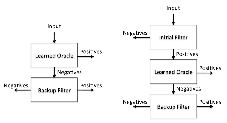
Figure 1: The left side shows the original learned Bloom filter. The right side shows the sandwiched learned Bloom filter.

The false positive rate of a sandwiched learned Bloom filter is then

$$\alpha^{b_{1}}(F_{p}+(1-F_{p})\alpha^{b_{2}/F_{n}}).$$

To see this, note that for $y\notin{\cal K}$, $y$ first has to pass through the initial Bloom filter, which occurs with probability $\alpha^{b_{1}}$. Then $y$ either causes a false positive from the learned function $f$ with probability $F_{p}$, or with remaining probability $(1-F_{p})$ it yields a false positive on the backup Bloom filter, with probability $\alpha^{b_{2}/F_{n}}$.

As $\alpha,F_{p},F_{n}$ and $b$ are all constants for the purpose of this analysis, we may optimize for $b_{1}$ in the equivalent expression

$$F_{p}\alpha^{b_{1}}+(1-F_{p})\alpha^{b/F_{n}}\alpha^{b_{1}(1-1/F_{n})}.$$

The derivative with respect to $b_{1}$ is

$$F_{p}(\ln\alpha)\alpha^{b_{1}}+(1-F_{p})\left(1-\frac{1}{F_{n}}\right)\alpha^{b/F_{n}}(\ln\alpha)\alpha^{b_{1}(1-1/F_{n})}.$$

This equals 0 when

$$\frac{F_{p}}{(1-F_{p})\left(\frac{1}{F_{n}}-1\right)}=\alpha^{(b-b_{1})/F_{n}}=\alpha^{b_{2}/F_{n}}.$$

This yields that the false positive rate is minimized when

$$b_{2}=F_{n}\log_{\alpha}\frac{F_{p}}{(1-F_{p})\left(\frac{1}{F_{n}}-1\right)}.$$

This result may be somewhat surprising, as here we see that $b_{2}$ is a constant, independent of $b$. That is, the number of bits used for the backup filter is not a constant fraction of the total budgeted number of bits $bm$, but a fixed number of bits; if the number of budgeted bits increases, one should simply increase the size of the initial Bloom filter as long as the backup filter is appropriately sized.

In hindsight, returning to the expression for the false positive rate

$$\alpha^{b_{1}}(F_{p}+(1-F_{p})\alpha^{b_{2}/F_{n}}),$$

we can see the intuition for why this would be the case. If we think of sequentially distributing the $bm$ bits among the two Bloom filters, the expression shows that bits assigned to the initial filter (the $b_{1}$ bits) reduce false positives arising from the learned function (the $F_{p}$ term) as well as false positives arising subsequent to the learned function (the $(1-F_{p})$ term), while the backup filter only reduces false positives arising subsequent to the learned function. Initially we would provide bits to the backup filter to reduce the $(1-F_{p})$ rate of false positives subsequent to the learned function. Indeed, bits in the backup filter drive down this $(1-F_{p})$ term rapidly, because the backup filter holds fewer keys from the original set, leading to the $b_{2}/F_{n}$ (instead of just a $b_{2}$) in the exponent in the expression $\alpha^{b_{2}/F_{n}}$. Once the false positives coming through the backup Bloom filter reaches an appropriate level, which, by plugging in the determined optimal value for $b_{2}$, we find is

$$F_{p}/\left(\frac{1}{F_{n}}-1\right),$$

then the tradeoff changes. At that point the gains from reducing the false positives from the backup Bloom filter are smaller than the gains obtained by using the initial Bloom filter.

As an example, using numbers roughly corresponding to settings tested in [2], suppose we have a learned function $f$ where $F_{n}=1/2$ and $F_{p}=1/100$. For convenience we consider $\alpha=1/2$ (that corresponds to perfect hash function based Bloom filters). Then

$$b_{2}=(\log_{2}99)/2\approx 3.315.$$

Depending on our Bloom filter budget parameter $b$, we obtain different levels of performance improvement by using the initial Bloom filter. At $b=8$ bits per key, the false positive rate drops from approximately $0.010015$ to $0.000777$, over an order of magnitude. Even at $b=6$ bits per key, the false positive rate drops from approximately $0.010242$ to $0.003109$.

If one wants to consider a fixed false positive rate and consider the space savings from using the sandwiched approach, that is somewhat more difficult. The primary determinant of the overall false positive rate is the oracle’s false positive probability $F_{p}$. The sandwich optimization allows one to achieve better overall false positive with a larger $F_{p}$; that is, it can allow for weaker, and correspondingly smaller, oracles.

A possible further advantage of the sandwich approach is that it makes learned Bloom filters more robust. As discussed in [3], if the queries given to a learned Bloom filter do not come from the same distribution as the queries from the test set used to estimate the learned Bloom filter’s false positive probability, the actual false positive probability may be substantially larger than expected. The use of an initial Bloom filter mitigates this problem, as this issue affects the smaller number of keys that pass the initial Bloom filter.

In any case, we suggest that given that the sandwich learned Bloom filter is a relatively simple modification if one chooses to use a learned Bloom filter, we believe that the sandwiching method will allow greater application of the learned Bloom filter methodology.

References

- [1] A. Broder and M. Mitzenmacher. Network applications of bloom filters: A survey. Internet Mathematics, 1(4):485-509, 2004.
- [2] T. Kraska, A. Beutel, E. H. Chi, J. Dean, and N. Polyzotis. The Case for Learned Index Structures. https://arxiv.org/abs/1712.01208, 2017.
- [3] M. Mitzenmacher. A Model for Learned Bloom Filters and Related Structures. https://arxiv.org/abs/1802.00884, 2018.