Supplementary Material for “Topological Sachdev-Ye-Kitaev Model”

I Self-consistent equation in the real time.

In this section, we would like to present the self-consistent equaton used in our numerics. The Hamiltonian is given by the Eq. (5) of the main text. Following the standard large-N analysis for the SYK model Comments , the only non-vaninshing diagram for the self-energy is shown in FIG. 1. The Schwinger-Dyson equation in the imaginary time is given by:

$$G^{-1}(i\omega_{n},\mathbf{p}) =-i\omega_{n}+h(\mathbf{p})-\Sigma(i\omega_{n}),$$ (1)

$$\Sigma(\tau) =\begin{pmatrix}\Sigma^{\uparrow}(\tau)&0\\ 0&\Sigma^{\downarrow}(\tau)\end{pmatrix},$$ (2)

with

$$\Sigma^{\sigma}(\tau)=J^{2}(G^{\sigma\sigma}(\tau))^{2}G^{\sigma\sigma}(-\tau).$$ (3)

The propagator $G$ here is defined as

$$\left(G(\tau,\mathbf{x})\right)^{\sigma\sigma^{\prime}}\delta_{\lambda\lambda^{\prime}}=\left<\mathcal{T}_{\tau}c_{i+\mathbf{x},\sigma\lambda}(\tau)c_{i,\sigma^{\prime}\lambda^{\prime}}(0)\right>,$$

and we have used a simplified notion $G_{\tau}(\tau)\equiv G(\tau,\mathbf{0})$. Following similar derivations as in Ref.Comments ; Altman ; our ; DPSYK ; Balent by doing an analytical continuation, we obtain the self-consistent equation for the retarded Green’s function $G_{R}(\mathbf{x},t)$ in the real time as

$$G_{R}^{-1}(p,\omega) =\omega-h(p)-\Sigma_{R}(\omega),$$ (4)

$$\Sigma_{R}(\omega) =\begin{pmatrix}\Sigma_{R}^{\uparrow}(\omega)&0\\ 0&\Sigma_{R}^{\downarrow}(\omega)\end{pmatrix},$$ (5)

where

$$\Sigma_{R}^{\sigma}(\omega)=-iJ^{2}\int_{0}^{\infty}dte^{i\omega t}((n_{1}^{\sigma}(t))^{2}n_{2}^{\sigma}(t)+(n_{3}^{\sigma}(t))^{2}n_{4}^{\sigma}(t)),$$ (6)

and

$$n_{1}^{\sigma}(t)=\int A^{\sigma}(\omega)n_{F}(-\omega)e^{-i\omega t}=n_{4}^{\sigma}(t)^{*},$$ (7)

$$n_{2}^{\sigma}(t)=\int A^{\sigma}(\omega)n_{F}(\omega)e^{i\omega t}=n_{3}^{\sigma}(t)^{*}.$$ (8)

$$A^{\sigma}(\omega)=-\frac{1}{\pi}\text{Im}\int\frac{d^{2}p}{(2\pi)^{2}}G_{R}^{\sigma\sigma}(p,\omega).$$ (9)

Here $A^{\sigma}$ is the spectral function of fermions. This set of equations can be directly solved numerically by iteration. To get correct zero-temperature result, one should be careful about the discretization of integrals, which will be discussed in the next section.

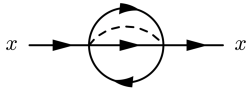
Figure 1: The self-energy diagram at the leading order of the large $N$ expansion for the Green’s function of fermions. The dashed line means the disorder average and the solid line is the full Green’s function of fermions.

II Finite size scaling.

When solving the self-consistent equation in the real time at $T=0$, the integration over time $t$ and frequency $\omega$ are approximated by a summation over finite number of points. This sets a cutoff which serves as an effective temperature. To obtain physical results at the zero temperature, we need to perform a finite size scaling to send the discretization $L$ to infinity. In this section we explain the details of this procedure.

In the numerics we take constant hopping $t_{0}$ to be the unit and the cutoff of the integration over frequency $\omega$ (time $t$) is given by $20t_{0}$ (20/$t_{0}$). We check that the result is robust against the change of this cutoff. The most sensitive parameter is the discretization $L$ when we fix the cutoff. Instead of a uniform discretization, to increase the accuracy, we implement the Gauss-Kronrod rule to approximate the integration to the $L$-th order and perform a finite size scaling in terms of $L$.

A typical result is shown in FIG. 2. We set $J/t_{0}=8$ and $m=2.5$. After a finite size scaling, it is clear from Fig. 2(a) that for sufficiently small $\omega$, $A(\omega)$ always scales to zero and the system is gapped. From Fig. 2(b) the peak also becomes sharper which indicates the effective temperature is lowered. We have also checked the sum rule of the spectral function that $\int d\omega A(\omega)=1$ is always satisfied with an error of $10^{-4}$ order.

III symmetry and its constrain to the self-energy.

In this section we show that because of the $\mathcal{P}$ symmetry defined as the Eq. (11) of the main text, there is a relation $\Sigma^{\uparrow}(0)=-\Sigma^{\downarrow}(0)$ when the self-energy at $\omega=0$ is real. Recalling the definition of the $\mathcal{P}$ symmetry:

$$\mathcal{P}c_{\mathbf{p}\sigma\lambda}\mathcal{P}^{-1}=(\sigma_{y})_{\sigma\sigma^{\prime}}c^{\dagger}_{\mathbf{p}\sigma^{\prime}\lambda},$$ (10)

now we study the constraint that it can impose on the Green’s function:

$$G(\omega=0,\mathbf{p})= \int d\tau\left<c_{\mathbf{p},\lambda}(\tau)c^{\dagger}_{\mathbf{p},\lambda}(0)\right>$$ (11)

$$= \int d\tau\left<\mathcal{P}\mathcal{P}^{-1}c_{\mathbf{p},\lambda}(\tau)\mathcal{P}\mathcal{P}^{-1}c^{\dagger}_{\mathbf{p},\lambda}(0)\mathcal{P}\mathcal{P}^{-1}\right>$$ (12)

$$= \int d\tau\ \sigma_{y}\left<c^{\dagger}_{\mathbf{p},\lambda}(\tau)c_{\mathbf{p},\lambda}(0)\right>(-\sigma_{y})$$ (13)

$$= \sigma_{y}G(\omega=0,\mathbf{p})\sigma_{y}$$ (14)

Here we have used the matrix representation by keeping the spin index implicit and we assume the ground state do not break the $\mathcal{P}$ symmetry. By taking the inverse of above identity, one obtains

$$G^{-1}(\omega=0,\mathbf{p})=\sigma_{y}G^{-1}(\omega=0,\mathbf{p})\sigma_{y}.$$ (15)

Knowing that $G^{-1}(\omega=0,\mathbf{p})=h(\mathbf{p})-\Sigma(0)$ and when the self energy is purely real, one reaches $\Sigma(0)=\sigma_{y}\Sigma(0)\sigma_{y}$ and thus $\Sigma(0)\propto\sigma_{z}$. Consequently, $\Sigma^{\uparrow}(0)=-\Sigma^{\downarrow}(0)$.

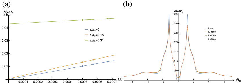
Figure 2: The numerical results for finite size scaling. (a). Spectral function at some frequency as a function of $1/L$ and the fitting to a straight line. (b). Spectral function for different $1/L$.

IV Understanding the phase boundary: a toy model for weak interaction.

In this section we aim at understanding the reason for why SYK interaction favors a topological nontrivial phase by a simple toy model. We approximate the original model by a simplified two-sites complex SYK model with single-particle mixing as

$$H=t_{0}\sum\limits_{\sigma\sigma^{\prime}}c^{\dagger}_{\sigma\lambda}(m\sigma_{z}+\delta\sigma_{x})_{\sigma\sigma^{\prime}}c_{\sigma^{\prime}\lambda}+\frac{1}{4}\sum\limits_{\sigma}\sum\limits_{\lambda_{1}\lambda_{2}\lambda_{3}\lambda_{4}}J_{\lambda_{1}\lambda_{2}\lambda_{3}\lambda_{4}}^{\sigma}c^{\dagger}_{\sigma\lambda_{1}}c^{\dagger}_{\sigma\lambda_{2}}c_{\sigma\lambda_{3}}c_{\sigma\lambda_{4}},$$ (16)

where $J_{\lambda_{1}\lambda_{2}\lambda_{3}\lambda_{4}}^{\sigma}$ satisfies the Gaussian distribution as the on-site random interaction in the original model. This toy model mimics the original model when $m\gg 1$ and if we could neglect the momentum dependence of the mixing between spins. Without random interaction, the retarded Green’s function is given by:

$$G_{0}(\omega)=\frac{\omega+mt_{0}\sigma_{z}+\delta t_{0}\sigma_{x}}{\omega^{2}-t_{0}^{2}m^{2}-t_{0}^{2}\delta^{2}}=\frac{\omega+mt_{0}\sigma_{z}+\delta t_{0}\sigma_{x}}{\omega^{2}-M^{2}t_{0}^{2}}.$$ (17)

Here we define $M=\sqrt{m^{2}+\delta^{2}}$. Focusing on fermions with spin $\uparrow$, without interaction, the spectral function is given by:

$$A^{\uparrow}(\omega)=-\frac{1}{\pi}\text{Im}G_{0}^{\uparrow\uparrow}(\omega)=\frac{M+m}{2M}\delta(\omega-Mt_{0})+\frac{M-m}{2M}\delta(\omega+Mt_{0}).$$ (18)

As given in Eq. (6), the self-energy for the retarded Green’s function is given by:

$$\Sigma(\omega)=-iJ^{2}\int_{0}^{\infty}dt\left(n_{1}(t)^{2}n_{2}(t)+n_{3}(t)^{2}n_{4}(t)\right)e^{i\omega t}.$$ (19)

Here $n_{i}(t)$ is given by:

$$n_{1}(t) =\int A(\omega)n_{F}(-\omega)e^{-i\omega t}d\omega=\frac{M+m}{2M}e^{-iMt_{0}t}=n_{4}(t)^{*},$$ (20)

$$n_{2}(t) =\int A(\omega)n_{F}(\omega)e^{i\omega t}d\omega=\frac{M-m}{2M}e^{-iMt_{0}t}=n_{3}(t)^{*}.$$ (21)

As a result one has:

$$m_{\text{eff}}=m-\frac{mJ^{2}\delta^{2}}{12t_{0}^{2}(m^{2}+\delta^{2})^{2}}.$$ (22)

Since random interaction shifts $|m|$ to be smaller, this effect stabilizes the topological phase. Physically, one could understand this by considering a single particle excitation with spin $\uparrow$. This single excitation, with energy $t_{0}|m|$, can be scattered to a state with two particles with spin $\uparrow$ and one hole with spin $\downarrow$, whose energy is $3t_{0}|m|$. As a result, the energy of a single excitation, $|m|$, is lowered.

V Calculation of conductance.

In this section we explain our method for calculating the conductance. We use the Keldysh contour to formulate the field theory directly in the real time to avoid the analytical continuation Kamenev . In the standard Keldysh approach there are two time contours $+/-$ and thus two copies of fields $c_{i,+}$ and $c_{i,-}$ (we drop flavor and spin indexes for simplicity). The phase fluctuation is introduced by $c_{i,\pm}\rightarrow\exp(-i\phi_{i,\pm})c_{i,\pm}$ with an assumption that $\phi_{i}$ is a smooth fluctuation approximated by $\phi_{\pm}(\mathbf{x})$ Balent ; DPSYK . We take the convention Kamenev :

$$c_{1}=\frac{1}{\sqrt{2}}(c_{+}+c_{-}),\ \ \ \ c_{2}=\frac{1}{\sqrt{2}}(c_{+}-c_{-}),$$ (23)

$$\overline{c}_{1}=\frac{1}{\sqrt{2}}(\overline{c}_{+}-\overline{c}_{-}),\ \ \ \ \overline{c}_{2}=\frac{1}{\sqrt{2}}(\overline{c}_{+}+\overline{c}_{-}),$$ (24)

$$\phi_{\text{cl}/q}=\frac{1}{2}(\phi_{+}\pm\phi_{-}),\ \ A_{\alpha,\text{cl}/q}=\frac{1}{2}(A_{\alpha,+}\pm A_{\alpha,-}).$$ (25)

Here $A_{i,\pm}$ are gauge fields introduced by minimal coupling to extract the current-current correlation function. In the low-energy limit, the coupling is given by:

$$S_{K}[A]= A_{\alpha,+}c_{+}^{\dagger}(\partial_{\alpha}h)c_{+}+\frac{1}{2}A_{\alpha,+}A_{\beta,+}c_{+}^{\dagger}(\partial_{\alpha}\partial_{\beta}h)c_{+}$$

$$-A_{\alpha,-}c_{-}^{\dagger}(\partial_{\alpha}h)c_{-}-\frac{1}{2}A_{\alpha,-}A_{\beta,-}c_{-}^{\dagger}(\partial_{\alpha}\partial_{\beta}h)c_{-}.$$ (26)

Here the partial derivative is for the corresponding component of momentums and we leave out the label of momentum for simplicity. Here we start with the standard Green’s function in Keldysh formalism:

$$\left<c_{i+\mathbf{x},\alpha}(t)\overline{c}_{i,\beta}(0)\right>=\begin{pmatrix}G_{R}(\mathbf{x},t)&G_{K}(\mathbf{x},t)\\ 0&G_{A}(\mathbf{x},t)\end{pmatrix},$$

where $G_{R}$/$G_{A}$/$G_{K}$ is the retarded/advanced/Keldysh Green’s function for fermions. We have $G_{K}(\mathbf{p},\omega)=(1-2n_{F}(\omega))(G_{R}(\mathbf{p},\omega)-G_{A}(\mathbf{p},\omega))$ in thermal equilibrium which is called the fluctuation-dissipation theorem. We have omitted the spin index and all the correlation function are matrix. The current and the retarded Green’s function for current operators are then given by:

$$J_{\alpha,\text{cl}}=-\frac{i}{2}\frac{\partial\ln Z}{\partial A_{\alpha,q}},\ \ \ \ \Pi_{R,\alpha\beta}=\frac{\partial J_{\alpha,\text{cl}}}{\partial A_{\beta,\text{cl}}}=-\frac{i}{2}\frac{\partial^{2}\ln Z}{\partial A_{\beta,\text{cl}}A_{\alpha,\text{q}}}.$$ (27)

The longitudinal conductance and the Hall conductance are then given by:

$$\sigma_{xx}= \lim_{\omega\rightarrow 0}\frac{1}{i\omega}\Pi_{R,xx}(\mathbf{0},\omega).$$ (28)

$$\sigma_{xy}= \lim_{\omega\rightarrow 0}\frac{1}{2i\omega}(\Pi_{R,xy}(\mathbf{0},\omega)-\Pi_{R,yx}(\mathbf{0},\omega)).$$ (29)

As any well-defined large-N model, after integrating out the fermions, the effective action is proporational to $N$: $S_{\text{eff}}\left[\phi\right]=NS^{\prime}_{\text{eff}}\left[\phi\right]$, because of which the Green’s function of $\phi$ is suppressed by $1/N$ Coleman . As a result, only the Gaussian fluctuation of $\phi$ is taken into account in the leading order of large-$N$ Balent ; DPSYK , and therefore it only requires the information of two-point correlation function of fermions computed in the previous sections. Following similar procedures as in Ref. DPSYK , we could derive

$$iS^{\prime}_{\text{eff}}\left[\phi,A_{\alpha}\right]= (D_{d}\delta^{\alpha\beta}+D_{pp}^{\alpha\beta})(\partial_{\alpha}\phi_{q}+A_{\alpha,q})(\partial_{\beta}\phi_{\text{cl}}+A_{\beta,\text{cl}})+D_{\omega\omega}\partial_{t}\phi_{\text{cl}}\partial_{t}\phi_{q}$$

$$+ D_{\omega p}^{\alpha}(\partial_{\alpha}\phi_{\text{cl}}+A_{\alpha,\text{cl}})\partial_{t}\phi_{q}+D_{\omega p}^{\prime\alpha}\partial_{t}\phi_{\text{cl}}(\partial_{\alpha}\phi_{q}+A_{\alpha,q}),$$ (30)

$$D^{\alpha\beta}_{pp}(\omega)= -\int\frac{dq_{0}d^{2}q}{(2\pi)^{3}}(\text{tr}\left[\frac{\partial h}{\partial q_{\alpha}}G_{R}(q_{0}+\omega,\mathbf{q})\frac{\partial h}{\partial q_{\beta}}G_{K}(q_{0},\mathbf{q})\right]+\text{tr}\left[\frac{\partial h}{\partial q_{\alpha}}G_{K}(q_{0}+\omega,\mathbf{q})\frac{\partial h}{\partial q_{\beta}}G_{A}(q_{0},\mathbf{q})\right]),$$ (31)

$$D_{\omega\omega}(\omega)= -\int\frac{dq_{0}d^{2}q}{(2\pi)^{3}}(\text{tr}\left[G_{R}(q_{0}+\omega,\mathbf{q})G_{K}(q_{0},\mathbf{q})\right]+\text{tr}\left[G_{K}(q_{0}+\omega,\mathbf{q})G_{A}(q_{0},\mathbf{q})\right]),$$ (32)

$$D^{\alpha}_{\omega p}(\omega)= -\int\frac{dq_{0}d^{2}q}{(2\pi)^{3}}(\text{tr}\left[\frac{\partial h}{\partial q_{\alpha}}G_{R}(q_{0}+\omega,\mathbf{q})G_{K}(q_{0},\mathbf{q})\right]+\text{tr}\left[\frac{\partial h}{\partial q_{\alpha}}G_{K}(q_{0}+\omega,\mathbf{q})G_{A}(q_{0},\mathbf{q})\right]),$$ (33)

$$D^{\prime\alpha}_{\omega p}(\omega)= -\int\frac{dq_{0}d^{2}q}{(2\pi)^{3}}(\text{tr}\left[G_{R}(q_{0}+\omega,\mathbf{q})\frac{\partial h}{\partial q_{\alpha}}G_{K}(q_{0},\mathbf{q})\right]+\text{tr}\left[G_{K}(q_{0}+\omega,\mathbf{q})\frac{\partial h}{\partial q_{\alpha}}G_{A}(q_{0},\mathbf{q})\right]).$$ (34)

Here we keep the label of freqency implicit and only show the retarded part of the action, and $D_{d}=-D_{pp}^{\alpha\alpha}(0)$ is the contribution from the diamagnetic term. In the zero momentum limit, one could show $D_{\omega p}^{\alpha}=D_{\omega p}^{\prime\alpha}=0$, we find now:

$$\sigma_{xx}= -\lim_{\omega\rightarrow 0}\frac{1}{2\omega}(D^{xx}_{pp}(\omega)-D^{xx}_{pp}(0)),$$ (35)

$$\sigma_{xy}= -\lim_{\omega\rightarrow 0}\frac{1}{4\omega}(D^{yx}_{pp}(\omega)-D^{xy}_{pp}(\omega)).$$ (36)

Eq.(36) is consistent with the exact result derived in Hall by using the Wald identity.

References

• (1) J. Maldacena and D. Stanford, Phys.Rev. D 94 (2016) 106002.
• (2) S. Banerjee and E. Altman, Phys. Rev. B 95, 134302.
• (3) X. Chen, R. Fan, Y. Chen, H. Zhai and P. Zhang, Phys. Rev. Lett. 119, 207603 (2017).
• (4) P. Zhang, Phys. Rev. B 96, 205138 (2017).
• (5) X.-Y. Song, C.-M. Jian and L. Balents, Phys. Rev. Lett. 119, 216601 (2017).
• (6) Z. Wang and S.-C. Zhang, Phys. Rev. X 2, 031008 (2012).
• (7) K. Ishikawa and T. Matsuyama, Z. Phys. C 33, 41 (1986).
• (8) A. Kamenev, Field theory of non-equilibrium systems, Cambridge University Press, 2011.
• (9) C. Coleman, “Aspect of symmetry: selected Erice Lectures of Sidney Coleman.” Cambridge University Press, 1985.