DFPD-2018/TH/01

Three-forms, dualities and membranes
in four-dimensional supergravity

Abstract

We consider four-dimensional ${\cal N}=1$ supergravity models of a kind appearing in string flux compactifications. It has been recently shown that, by using double three-form multiplets instead of ordinary chiral multiplets, one can promote to dynamical variables (part of) the quantized numbers appearing in the flux-induced superpotential. We show that double three-form multiplets naturally transform under symplectic dualities associated with the special Kähler structure that characterizes their scalar sector. Furthermore, we discuss how to couple membranes which carry arbitrary ‘electric-magnetic’ charges. The complete action is supersymmetric, kappa-symmetric and duality covariant. As an application, we derive the flow equations for BPS domain walls sourced by membranes and give simple analytic examples of their solution.

^† Department of Theoretical Physics, University of the Basque Country UPV/EHU, P.O. Box 644, 48080 Bilbao, Spain
^‡ IKERBASQUE, Basque Foundation for Science, 48011, Bilbao, Spain
^♠ KU Leuven, Institute for Theoretical Physics, Celestijnenlaan 200D,
B-3001 Leuven, Belgium
^∗ Dipartimento di Fisica e Astronomia “Galileo Galilei", Università degli Studi di Padova,
Via F. Marzolo 8, 35131 Padova, Italy
^♢ I.N.F.N. Sezione di Padova, Via F. Marzolo 8, 35131 Padova, Italy

1 Introduction

In recent years the role of gauge three-forms in four-dimensional effective theories has been revisited in various contexts and from different perspectives. In particular, three-forms can provide an effective dynamical ‘Hodge-dual’ description of the internal flux quanta which specify certain classes of string flux compactifications. The inclusion of gauge three-forms in effective theories may have interesting physical effects, such as the dynamical generation of the cosmological constant and its neutralization [1, 2, 3, 4, 5, 6, 7, 8, 9, 10, 11, 12, 13, 14, 15], the contribution to inflationary scenarios [16, 17, 18, 19, 20, 21], possible resolution of the strong CP violation problem [22, 23, 24, 25, 26, 27] and others.

In [28] it was shown how to construct generic ${\mathcal{N}}=1$ supergravity models in the presence of gauge three-forms. The construction naturally applies to supergravities with a scalar sector described by a special Kähler geometry. This is indeed often the case for stringy effective theories, as the ones considered in [19, 29, 30], which studied the role of gauge three-forms in the context of type II compactifications. The link between double three-forms and the moduli parametrizing a special Kähler space can be understood, for instance, by thinking of type IIB theory on a Calabi–Yau three-fold and focusing on the special Kähler space parametrized by its complex structure moduli. As usual, one can consider a symplectic basis of internal CY three-cycles $(\Pi^{I},\tilde{\Pi}_{J})$ ($I,J=0,\ldots,n$) and parametrize the complex structures moduli by projective coordinates $s^{I}\equiv\int_{\Pi^{I}}\Omega$, where $\Omega$ is the holomorphic CY $(3,0)$ form[31]. On the other hand, by integrating the Ramond-Ramond (R-R) six-forms on $(\Pi^{I},\tilde{\Pi}_{J})$ one gets a set of associated double three-forms $(A^{I}_{3},\tilde{A}_{3I})$ in four-dimensions. Now, this and similar settings are characterized by a symplectic duality group associated with the special Kähler geometry, which in this example corresponds just to the group of possible symplectic rotations of the basis $(\Pi^{I},\tilde{\Pi}_{J})$. These transformations mix up the coordinates $s^{I}$ with the dual coordinates ${\cal G}_{I}(s)\equiv\int_{\tilde{\Pi}_{I}}\Omega$. At the same time, they should act on the double three-forms $(A^{I}_{3},\tilde{A}_{3I})$ as well, rotating them as electric-magnetic pairs.

These observations may be extrapolated to other less supersymmetric examples, with orientifolds and internal fluxes, whose effective theory can be described by an ${\cal N}=1$ supergravity with double three-form multiplets of the form derived in [28], or a variation thereof. The double three-form multiplets contain a complex scalar and a pair of three-forms, which will be denoted by $s^{I}$ and $(A^{I}_{3},\tilde{A}_{3J})$ as in the above example. We then expect these supergravities to naturally accommodate the action of the symplectic group associated with the relevant special Kähler structure. In this paper we show that this is indeed the case: the symplectic group has a natural action on the double three-form multiplets and the effective supergravity is covariant under it.

Since our supersymmetric formulation contains three-form gauge potentials, it is also quite natural to consider the corresponding charged objects, namely membranes sweeping three-dimensional world-volumes ${\cal C}$. By requiring compatibility with the symplectic transformations, they should couple to the three-forms through a bosonic minimal-coupling term of the form

$$q_{I}\int_{\cal C}A^{I}_{3}-p^{I}\int_{\cal C}\tilde{A}_{3I}\,,$$ (1.1)

where $(p^{I},q_{J})$ denote a symplectic vector of quantized electro-magnetic charges, which rotate under the action of the symplectic duality group. For instance, in the above type IIB example, a $(p^{I},q_{J})$-membrane would correspond to a D5-brane wrapping an internal three-cycle $\Pi$ homologous to $q_{I}\Pi^{I}-p^{I}\tilde{\Pi}_{I}$.

Such membranes can be coupled in a manifestly supersymmetric way to the bulk sector of our four-dimensional effective supergravity. Indeed, we will show how to construct an action for a supermembrane in a curved superspace which couples to the bulk three-forms as in (1.1). This action contains a Nambu–Goto (NG) and a Wess–Zumino (WZ) term and is $\kappa$-symmetric, generalizing previously constructed supermembrane actions in four dimensions [32, 8, 33, 12, 13, 14, 34] and analogous superstring actions with two-form couplings in $D=3$ [35]. The WZ term, which is the supersymmetric completion of (1.1), will be defined by constructing appropriate super-three-forms from the three-form multiplets. On the other hand, the NG term will be uniquely fixed by requiring that the membrane action is $\kappa$-symmetric and hence supports a supersymmetric spectrum. The result is that the tension $T_{M}$ of the $(p^{I},q_{J})$-membrane is not a constant but rather depends on the scalar sector of the theory, namely

$$T_{M}=2\left|q_{I}s^{I}-p^{I}{\cal G}_{I}(s)\right|\,.$$ (1.2)

Note that, in the above type IIB example, this formula precisely matches the effective tension of the wrapped D5-branes, which is given by the volume of the internal cycle $\Pi$. Indeed, the BPS condition corresponds to a calibration condition [36] which implies that $T_{M}=\left|\int_{\Pi}\Omega\right|=\big{|}q_{I}\int_{\Pi^{I}}\Omega-p^{I}\int_{\tilde{\Pi}_{I}}\Omega\big{|}$, hence reproducing (1.2). This observation can be easily extended to more general and less supersymmetric type II flux compactifications on generalized Calabi-Yau spaces [37, 38].

We will provide explicit examples of $\mathcal{N}=1$ supergravity models coupled to double three-form multiplets and supermembranes. These include the effective theory resulting from type IIA compactifications with R-R fluxes. We stress that, differently from what happens for strings and branes in String Theory and M-theory, in four dimensions the membrane $\kappa$-symmetry does not require the bulk sector to obey any dynamical equations. To be precise, $\kappa$-symmetry imposes a set of off-shell constraints on the curved target superspace torsion which does not result in any equations of motion for the gravity or matter multiplets. This allows us to consider interacting systems in which the supermembrane back-reacts on the dynamical ‘bulk’ supergravity sector. Particular examples of such systems, namely a supermembrane interacting with a single three-form matter multiplet and with single three-form supergravity were proposed and studied in [12] and [13, 14], respectively.

In this paper we discuss in detail the general structure of BPS domain wall configurations arising in the supergravity theories under consideration, which significantly enlarge the class of domain walls previously described in an ordinary chiral matter-coupled supergravity [39, 40, 41, 42, 43, 44] and in a three-form supergravity [8, 33].

We think that the actions constructed in this paper provide an appropriate framework for describing, from an effective four-dimensional perspective, non-trivial dynamical processes involving at the same time membranes, fluxes and the scalar sector of flux compactifications, as for instance those considered in [9, 10].

The paper is organized as follows. In Section 2 we review one of the main results of [28], showing how to trade a chiral matter-coupled ${\cal N}=1$ supergravity for a dual theory that contains double three-form multiplets. In Section 3 we specialize to the case where the kinetic terms for the double three-form multiplets are defined by an underlying special Kähler geometry. These theories are naturally covariant under special Kähler symplectic tranformations, under which the gauge three-forms rotate as symplectic vectors. We also discuss the quantization of vacuum expectation values of four-form fluxes in purely four-dimensional setting. In Section 5 we study the coupling (1.1) of the gauge (super) three-forms to supersymmetric membranes. The requirement of the supermembrane action to be invariant under local $\kappa$-symmetry fixes its Nambu-Goto term such that the corresponding tension has the form (1.2).

With all the ingredients settled, in Section 6 we consider the complete bulk-plus-membrane action and study BPS domain walls interpolating between different supersymmetric vacua separated by the membrane. The vevs of the four-form fluxes are discontinuous (i.e. ‘jump’) across the membrane. When the three-forms are integrated out, they give rise to two different (disconnected) effective scalar field superpotentials on each side of the membrane. We will see that, as expected, for BPS domain walls the tension (1.2) precisely balances the minimal-coupling term (1.1) which cancel out in the complete bulk-plus-membrane BPS action, whose on-shell value depends only on the asymptotic vacua.

In Sections 7 and 8 we study a simple model involving only two double three-form multiples, hence containing four three-form gauge potentials. This model has a single vacuum for each choice of the four-form field-strength integration constants, and domain walls interpolate between the two different vacua separated by the membrane. We explicitly construct analytic solutions describing these domain walls.

In the Appendices, we collect additional results. In particular, in Appendix D we provide the complete proof of $\kappa$-symmetry for the supermembrane action and in Appendix E we describe the extension of this result to supermembranes coupled to more general bulk sectors including single three-form multiples.

2 Supergravity with double three-forms

In order to make this paper self-contained and to set the notation, in this section we briefly review the structure of the ${\cal N}=1$ supergravity with three-form multiplets constructed in [28]. We will focus on the locally supersymmetric case with double three-form multiplets, but the construction under consideration can be easily adapted to the rigid case and/or to the other kinds of three-form multiplets studied e.g. in [45, 46, 47, 8, 48, 12, 13, 14, 28, 34, 49, 50]. Some of such examples are described in Appendix E.

Consider a general ${\cal N}=1$ supergravity theory describing the coupling of the gravity multiplet to a set of chiral multiplets $(Z^{I},T^{r})$, with $I=0,\ldots,n$ and $r=1,\ldots,m$. As in [28], we start from the super-conformally invariant approach [51, 52, 53] (see e.g. [54] for details) by including in $Z^{I}$ a conformal compensator such that the scaling dimension of $Z^{I}$ is $\Delta_{Z}=3$, while $T^{r}$ are assumed to have vanishing scaling dimension, $\Delta_{T}=0$. Furthermore, we assume that $Z^{I}$ can be regarded as projective coordinates of a special Kähler manifold locally specified by a homogeneous prepotential ${\cal G}(Z)$ such that ${\cal G}(\lambda Z)=\lambda^{2}{\cal G}(Z)$, for any arbitrary chiral superfield $\lambda$. We can now write the supergravity Lagrangian in the form

$${\cal L}^{\prime}=-3\int\text{d}^{4}\theta\,E\,\Omega(Z,\bar{Z};T,\bar{T})+\left(\int\text{d}^{2}\Theta\,2{\cal E}\,{\cal W}(Z;T)+c.c.\right)\,.$$ (2.1)

Super-Weyl invariance requires that the ‘kinetic’ superfield $\Omega(Z,\bar{Z};T,\bar{T})$ has scaling dimension $\Delta_{\Omega}=2$, while the superpotential ${\cal W}(Z;T)$ has scaling dimension $\Delta_{\cal W}=3$, which means

$$\Omega(\lambda Z,\bar{\lambda}\bar{Z};T,\bar{T})=|\lambda|^{\frac{2}{3}}\Omega(Z,\bar{Z};T,\bar{T})\,,\quad{\cal W}(\lambda Z,T)=\lambda{\cal W}(Z,T).$$ (2.2)

Furthermore, we split ${\cal W}(Z;T)$ as follows

$${\cal W}(Z;T)=e_{I}Z^{I}-m^{I}{\cal G}_{I}(Z)+\hat{\cal W}(Z;T),$$ (2.3)

where ${\cal G}_{I}(Z)\equiv\partial_{I}{\cal G}(Z)={\cal G}_{IJ}Z^{J}$, ${\cal G}_{IJ}\equiv\partial_{I}\partial_{J}{\cal G}(Z)$, etc., and $\hat{\cal W}(\lambda Z;T)=\lambda\hat{\cal W}(Z;T)$. It is instructive to notice that the homogeneity requirements imply

$${\cal G}_{I}(Z)={\cal G}_{IJ}(Z)Z^{J}\;,\qquad{\cal G}_{IJK}(Z)Z^{K}=0\;.\quad$$ (2.4)

At this point, one may fix the super-Weyl invariance and get a standard supergravity action. However, by preserving super-Weyl invariance one can more easily derive from (2.1) a dual theory in which the constants $(m^{I},e_{J})$ are promoted to the (Hodge-dual of the) field strengths of gauge three-forms. In short (we refer to [28] for details), to get the dual Lagrangian one removes the terms $e_{I}Z^{I}-m^{I}{\cal G}_{I}(Z)$ from the superpotential (2.3) and substitutes $Z^{I}$ with special chiral superfields $S^{I}$ constructed as follows

$$S^{I}\equiv\frac{1}{4}(\bar{\cal D}^{2}-8{\cal R}){\cal M}^{IJ}(\Sigma_{J}-\bar{\Sigma}_{J}).$$ (2.5)

Here ${\cal M}^{IJ}$ is the inverse of

$${\cal M}_{IJ}\equiv{\rm Im\hskip 1.00006pt}{\cal G}_{IJ}$$ (2.6)

and $\Sigma_{I}$ are complex linear superfields, i.e. they satisfy

$$(\bar{\cal D}^{2}-8{\cal R})\Sigma_{I}=0.$$ (2.7)

Note that ${\cal G}_{IJ}$ and ${\cal M}_{IJ}$, which were functions of $Z^{I}$ and $\bar{Z}{}^{I}$, should now be considered as functions of $S^{I}$ and $\bar{S}^{I}$. The new Lagrangian takes the form

$${\cal L}=-3\int\text{d}^{4}\theta\,E\,\Omega(S,\bar{S};T,\bar{T})+\left(\int\text{d}^{2}\Theta\,2{\cal E}\,\hat{\cal W}(S;T)+c.c.\right)+{\cal L}_{\rm bd},$$ (2.8)

where ${\cal L}_{\rm bd}$ is an appropriate boundary term which is necessary for having a well defined variational problem [28].

The complex linear superfields $\Sigma_{I}$ contain the double three-form multiplets, while the chiral superfields $S^{I}$ can be interpreted as multiplets of the corresponding field-strengths. Indeed, they are invariant under the gauge transformations

$$\Sigma_{I}\quad\rightarrow\quad\Sigma_{I}+\tilde{L}_{I}-{\cal G}_{IJ}L^{J}\,,$$ (2.9)

where $(L^{I},\tilde{L}_{J})$ are arbitrary real linear superfield parameters which supersymmetrize the three-form gauge transformations. We may partially fix (2.9) by imposing a Wess-Zumino gauge in which, in particular, $\Sigma_{I}|=0$. The remaining bosonic degrees of freedom contained in $\Sigma_{I}$ are given by complex scalars ${\tt s}_{I}$ and double (real) three-forms $(A^{I}_{3},\tilde{A}_{3J})$, which appear in the components

$${\cal D}^{2}\Sigma_{I}| =-4\bar{\tt s}_{I},$$ (2.10)

$$\bar{\sigma}_{m}^{\dot{\alpha}\alpha}[{\cal D}_{\alpha},\bar{\cal D}_{\dot{\alpha}}]\Sigma_{I}\big{|} =-2\big{(}{}^{*}\!\tilde{A}_{3I}-{\cal G}_{IJ}{}^{*}\!A_{3}^{J}\big{)}_{m}.$$

The residual gauge freedom in (2.9) corresponds to the standard gauge transformations $A^{I}_{3}\rightarrow A^{I}_{3}+\text{d}\Lambda^{I}_{2}$ and $\tilde{A}_{3J}\rightarrow\tilde{A}_{3J}+\text{d}\tilde{\Lambda}_{2J}$, where $(\Lambda^{I}_{2},\tilde{\Lambda}_{2J})$ are arbitrary two-forms.

The lowest components of the chiral superfields $S^{I}$ (2.5) are related to (2.10) as follows

$$S^{I}|\equiv s^{I}={\cal M}^{IJ}(s,\bar{s}){\mathtt{s}}_{J}.$$ (2.11)

On the other hand, if we put to zero the fermions, the field-strengths $F^{I}_{4}\equiv\text{d}A^{I}_{3}$ and $\tilde{F}_{4J}\equiv\text{d}\tilde{A}_{3J}$ enter the $S^{I}$ highest component as follows

$$F^{I}_{S}\equiv-\frac{1}{4}{\cal D}^{2}S^{I}|=\bar{M}s^{I}-\frac{{\rm i}}{2}\,{\cal M}^{IJ}{}^{*}\!{\cal F}_{4J}\,,$$ (2.12)

where $M$ is the complex scalar auxiliary field of the supergravity multiplet and

$${\cal F}_{4I}\equiv\tilde{F}_{4I}-\bar{\cal G}_{IJ}F_{4}^{J}\,$$ (2.13)

are complex four-forms with $\tilde{F}_{4I}=\text{d}\tilde{A}_{3I}$ and $F_{4}^{J}=\text{d}A_{3}^{J}$.

It is straightforward to extract from (2.8) the component Lagrangian and fix the super-Weyl invariance, finally obtaining, in the Einstein frame, supergravity with double three-forms, scalars and their fermionic partners. In the following sections we will restrict to a particular subclass of models.

3 A special subclass of models

Let us now assume that the kinetic function $\Omega$ has the factorized structure

$$\Omega(S,\bar{S};T,\bar{T})=\Omega_{0}(S,\bar{S})e^{-\frac{1}{3}\hat{K}(T,\bar{T})}\,,$$ (3.1)

where $\Omega_{0}(S,\bar{S})$ is defined by the special Kähler structure as follows

$$\Omega_{0}(S,\bar{S})=\left[{\rm i}\bar{S}^{I}{\cal G}_{I}(S)-{\rm i}S^{I}\bar{\cal G}_{I}(\bar{S})\right]^{\frac{1}{3}}\,.$$ (3.2)

Furthermore, in order to simplify the presentation, we will take $\hat{\cal W}(S,T)\equiv 0$, so that the superpotential of the original theory is just given by ${\cal W}(Z)=e_{I}Z^{I}-m^{I}{\cal G}_{I}(Z)$. A non-trivial $\hat{\cal W}(S,T)$ may be easily incorporated by using the general results of Appendix B. The corresponding theory with the double three-form multiplets is then described by the Lagrangian

$${\cal L}=-3\int\text{d}^{4}\theta\,E\,\Omega_{0}(S,\bar{S})e^{-\frac{1}{3}\hat{K}(T,\bar{T})}+{\cal L}_{\rm bd}\,.$$ (3.3)

Having in mind the symplectic invariance discussed in the following section, we will gauge fix super-Weyl symmetry in a slightly more flexible way than in [28].

Let us first express $S^{I}$ in terms of new chiral superfields $Y$ and $\Phi^{i}$, with $i=1,\ldots,n$, as follows

$$S^{I}=Y\,f^{I}(\Phi)\,,$$ (3.4)

where $f^{I}(\Phi)$ are holomorphic functions of $\Phi^{i}$ such that $\text{rank}(\partial_{i}f^{I})=n$. We assume that the new fields have scaling dimensions $\Delta_{Y}=3$ and $\Delta_{\Phi}=0$, so that $Y$ can be regarded as the compensator. $Y$ and $\Phi^{i}$ are not generic chiral superfields but rather have a constrained form, which can be in principle obtained by expressing them in terms of $S^{I}$ and then using (2.5).

We can then write

$$\Omega_{0}(S,\bar{S})=|Y|^{\frac{2}{3}}e^{-\frac{1}{3}K(\Phi,\bar{\Phi})}\,,$$ (3.5)

where

$$K(\Phi,\bar{\Phi}) =-\log\left[{\rm i}\bar{f}^{I}(\bar{\Phi}){\cal G}_{I}(\Phi)-{\rm i}f^{I}(\Phi)\bar{\cal G}_{I}(\bar{\Phi})\right]$$ (3.6)

$$=-\log\left[-2{\cal M}_{IJ}(\Phi,\bar{\Phi})f^{I}(\Phi)\bar{f}^{J}(\bar{\Phi})\right]\,,$$

with ${\cal G}_{I}(\Phi)\equiv{\cal G}_{I}(f(\Phi))$. We can now fix the super-Weyl gauge symmetry by imposing, for instance,

$$Y=1\,,$$ (3.7)

so that the Lagrangian becomes

$${\cal L}=-3\int\text{d}^{4}\theta\,E\,e^{-\frac{1}{3}{\cal K}(\Phi,\bar{\Phi},T,\bar{T})}+{\cal L}_{\rm bd}\,,$$ (3.8)

where

$${\cal K}(\Phi,\bar{\Phi},T,\bar{T})\equiv K(\Phi,\bar{\Phi})+\hat{K}(T,\bar{T})\,.$$ (3.9)

Of course there is a freedom in the choice of (3.4). This can be associated with the possibility of redefining $Y\rightarrow e^{g(\Phi)}Y$ and $f^{I}(\Phi)\rightarrow e^{-g(\Phi)}f^{I}(\Phi)$, which corresponds to a Kähler transformation

$$K\rightarrow K+g(\Phi)+\bar{g}(\bar{\Phi})\,.$$ (3.10)

3.1 Bosonic action

In order to express this Lagrangian in components, one should take into account (2.5) and (3.7). For simplicity, let us focus on the bosonic sector, setting all fermions to zero and writing $Y=y+\Theta^{2}F_{Y}$ and $\Phi^{i}=\phi^{i}+\Theta^{2}F^{i}_{\Phi}$. From (3.4) it follows that

$$F^{I}_{S}=f^{I}(\phi)F_{Y}+yf^{I}{}_{i}(\phi)F^{i}_{\Phi},$$ (3.11)

where $f^{I}{}_{i}(\phi)\equiv\frac{\partial}{\partial\phi^{i}}f^{I}(\phi)\equiv\partial_{i}f^{I}(\phi)$ . Then (3.7) is equivalent to $y=1$, i.e. $s^{I}=f^{I}(\phi)$, and $F^{I}_{S}=f^{I}{}_{i}F^{i}_{\Phi}$. In turn, by recalling (2.12), the latter is equivalent to

$$f^{I}(\phi)\bar{M}-f^{I}{}_{i}(\phi)F^{i}_{\Phi}=\frac{{\rm i}}{2}\,{\cal M}^{IJ}{}^{*}\!{\cal F}_{4J}.$$ (3.12)

Since we are assuming that the change of coordinates (3.4) is well defined, the $(n+1)\times(n+1)$ matrix $(f^{I},f^{I}{}_{i})$ is invertible and then (3.12) can be inverted to express $M$ and $F^{i}_{\Phi}$ in terms of the field-strengths $(F^{I}_{4},\tilde{F}_{4J})$. Note that ${\cal M}^{IJ}$ and ${\cal G}_{JK}$ should now be considered as functions of $(\phi^{i},\bar{\phi}^{\bar{\imath}}$).

Upon expanding (3.8) in bosonic components, performing the usual Weyl rescaling

$$e^{a}_{m}\to e^{a}_{m}e^{\frac{1}{6}{\cal K}}\,,\qquad(F^{i}_{\Phi},F^{q}_{T},M)\to e^{-\frac{2}{3}{\cal K}}(F^{i}_{\Phi},F^{q}_{T},M)$$ (3.13)

to pass to the Einstein frame, integrating out $F^{q}_{T}$ and using (3.12), we arrive at the bosonic action

$$S_{\rm bos}= -\int\text{d}^{4}x\,e\Big{(}\frac{1}{2}R+G_{IJ}f^{I}{}_{i}\bar{f}^{J}{}_{\bar{\jmath}}\;\partial\phi^{i}\partial\bar{\phi}^{\bar{\jmath}}+\hat{K}_{p\bar{q}}\,\partial t^{p}\partial\bar{t}^{\bar{q}}-{\cal T}^{IJ}{}^{*}{}\!\bar{\cal F}_{4I}{}^{*}{}\!{\cal F}_{4J}\Big{)}+S_{\rm bd}$$ (3.14)

with the boundary term

$$S_{\rm bd} =\,2{\rm Re\hskip 1.00006pt}\int_{\cal B}{\cal T}^{IJ}(\tilde{A}_{3I}-{\cal G}_{IK}A_{3}^{K})\,{}^{*}\!{\cal F}_{4J}$$ (3.15)

$$=-2{\rm Re\hskip 1.00006pt}\int\text{d}^{4}x\,e\,\nabla_{m}\left[{\cal T}^{IJ}\big{(}{}^{*}\!\tilde{A}_{3I}-{\cal G}_{IK}{}^{*}\!A_{3}^{K}\big{)}^{m}\,{}^{*}\!{\cal F}_{4J}\right],$$

where ${\cal B}$ is a space-time boundary (at infinity). In the above action, we have introduced the following quantities

$$G_{IJ} \equiv-\frac{{\cal M}_{IJ}}{(f{\cal M}\bar{f})}+\frac{({\cal M}\bar{f})_{I}({\cal M}f)_{J}}{(f{\cal M}\bar{f})^{2}},$$ (3.16a)

$${\cal T}^{IJ} \equiv\frac{1}{4}\,e^{-{\cal K}}\left[{\cal M}^{IK}G_{LK}{\cal M}^{LJ}+\frac{1}{\gamma}\frac{f^{I}\bar{f}^{J}}{(f{\cal M}\bar{f})^{2}}\right],$$ (3.16b)

$$\gamma \equiv\hat{K}_{\bar{q}}\hat{K}^{\bar{q}p}\hat{K}_{p}-3$$ (3.16c)

with $({\cal M}f)_{I}\equiv{\cal M}_{IJ}f^{J}$, $({\cal M}\bar{f})_{I}\equiv{\cal M}_{IJ}\bar{f}^{J}$ and $(f{\cal M}\bar{f})\equiv f^{I}{\cal M}_{IJ}\bar{f}^{J}$. The inverse matrix of ${\cal T}^{IJ}$ defined by ${\cal T}_{IJ}{\cal T}^{JK}={\cal T}^{KJ}{\cal T}_{JI}=\delta_{I}^{K}$ has the following form

$${\cal T}_{IJ}=-4e^{\cal K}\left[(f{\cal M}\bar{f}){\cal M}_{IJ}-(1+\gamma)({\cal M}f)_{I}({\cal M}\bar{f})_{J}\right]\,.$$ (3.17)

Clearly, $\gamma$ must be non-vanishing in order for the above action to make sense. Indeed, in deriving (3.14) a vanishing $\gamma$ would imply an obstruction in integrating out the auxiliary fields of the ‘spectator’ chiral multiplets $T^{p}$. In the following, we will assume that $\gamma$ is non-vanishing and constant. For instance, in the case of type II orientifold compactifications one finds $\gamma=1$ [56, 57]. Or, in the absence of a spectator sector, we have $\gamma=-3$.

Note that $\overline{G_{IJ}}=G_{JI}$, $f^{I}G_{IJ}=G_{JI}\bar{f}^{I}\equiv 0$ and $\overline{{\cal T}^{IJ}}={\cal T}^{JI}$. Furthermore, the special Kähler structure requires that ${\cal M}_{IJ}f^{I}\bar{f}^{J}<0$ and that the kinetic matrix $G_{IJ}f^{I}{}_{i}\bar{f}^{J}{}_{\bar{\jmath}}$ is positive definite, see for instance [58]. Note also that

$$K^{\bar{k}l}\bar{f}^{K}_{\bar{k}}f^{L}_{l}G_{IK}G_{LJ}=G_{IJ}.$$ (3.18)

This can be verified by projecting the first and second index along the complete bases $(f^{I},f^{I}_{i})$ and $(\bar{f}^{J},\bar{f}^{J}_{\bar{\jmath}})$, respectively, and recalling that $K_{i\bar{\jmath}}=G_{IJ}f^{I}_{i}\bar{f}^{J}_{\bar{\jmath}}$.

The three-form equations of motion are

$$\text{d}\,{\rm Re\hskip 1.00006pt}({\cal T}^{IJ}{}^{*}\!{\cal F}_{4J})=0\,,\quad\text{d}\,{\rm Re\hskip 1.00006pt}({\cal G}_{IJ}{\cal T}^{JK}{}^{*}\!{\cal F}_{4K})=0\,.$$ (3.19)

These equations imply that ${\rm Re\hskip 1.00006pt}({\cal T}^{IJ}{}^{*}\!{\cal F}_{4J})$ and ${\rm Re\hskip 1.00006pt}({\cal G}_{IJ}{\cal T}^{JK}{}^{*}\!{\cal F}_{4K})$ are constant, at least away from the membrane sources introduced below, namely

$$2{\rm Re\hskip 1.00006pt}({\cal T}^{IJ}{}^{*}\!{\cal F}_{4J})=m^{I}\,,\qquad 2{\rm Re\hskip 1.00006pt}({\cal G}_{IJ}{\cal T}^{JK}{}^{*}\!{\cal F}_{4K})=e_{I},$$ (3.20)

or equivalently

$${\cal T}^{IJ}{}^{*}\!{\cal F}_{4J}=-\frac{{\rm i}}{2}{\cal M}^{IJ}(e_{J}-\bar{\cal G}_{JK}m^{K}),$$ (3.21)

where $m^{I},e_{J}$ are real constants.

Consistent boundary conditions require the same combinations of the four-forms and scalars to take the fixed constant value on the boundary ${\cal B}$. One can then check that, indeed, the boundary term (3.15) makes the variational principle well defined, see for instance [5, 59] for a discussion of this issue in simpler settings.

3.2 Duality to standard matter-coupled supergravity

Let us now explicitly check the relation of the above formulation to the ordinary bosonic supergravity action (in the absence of membranes). First, we notice that the part of the action (3.14) containing the three-forms can be written in the following form

$$S_{\text{3-forms}} =\int\text{d}^{4}x\,e\,{\cal T}^{IJ}{}^{*}\!\bar{\cal F}_{4I}\,{}^{*}\!{\cal F}_{4J}+S_{\rm bd}$$ (3.22)

$$=-\int\text{d}^{4}x\,e\,{\cal T}^{IJ}{}^{*}\!\bar{\cal F}_{4I}\,{}^{*}\!{\cal F}_{4J}$$

$$\quad-2\int\Big{[}\tilde{A}_{3I}\wedge\text{d}\,{\rm Re\hskip 1.00006pt}({\cal T}^{IJ}{}^{*}\!{\cal F}_{4J})-A^{I}_{3}\wedge\text{d}\,{\rm Re\hskip 1.00006pt}({\cal G}_{IJ}{\cal T}^{JK}{}^{*}\!{\cal F}_{4K})\Big{]}.$$

For further comparison with the conventional supergravity action let us define the following quantities

$$W_{I} \equiv-2{\rm i}{\cal M}_{IJ}{\cal T}^{KJ}{}^{*}\!\bar{\cal F}_{4K},$$ (3.23a)

$$W \equiv f^{I}W_{I}=\frac{{\rm i}}{\gamma}e^{-\hat{K}}\left(f^{I}{}^{*}\tilde{F}_{4I}-{\cal G}_{I}{}^{*}F^{I}_{4}\right),$$ (3.23b)

$$W_{i} \equiv f_{i}^{I}W_{I}\,.$$ (3.23c)

At the moment this is just a change of variables, but we will shortly see that $W$ is associated with the superpotential of the conventional supergravity.

By using the relations (3.16a)-(3.18) it can be checked that the scalar potential, which is given by

$$V\equiv{\cal T}^{IJ}{}^{*}\!\bar{\cal F}_{4I}\,{}^{*}\!{\cal F}_{4J}$$ (3.24)

can be more explicitly written as follows

$$\begin{split}V&=e^{\cal K}\left[(f{\cal M}\bar{f})^{2}{\cal M}^{IK}{\cal M}^{JL}G_{LK}W_{I}\overline{W}_{\bar{J}}+\gamma|W|^{2}\right]\\ &=e^{\cal K}\left(K^{i\bar{\jmath}}(W_{i}+K_{i}W)(\overline{W}_{\bar{\jmath}}+K_{\bar{\jmath}}\overline{W})+\gamma|W|^{2}\right).\end{split}$$ (3.25)

Now, if the four-forms satisfy the equations (3.19)-(3.21), the action (3.22) reduces to

$$\begin{split}S_{\text{3-forms}}&=-\int\text{d}^{4}x\,e\,{\cal T}^{IJ}{}^{*}\!\bar{\cal F}_{4I}\,{}^{*}\!{\cal F}_{4J}\\ &\equiv-\int\text{d}^{4}x\sqrt{-g}\,V(\phi,\bar{\phi},t,\bar{t};e,m)\,,\quad~{}~{}~{}\text{(on-shell 3-forms)}\end{split}$$ (3.26)

which corresponds to an effective potential $V$ for the scalar fields, in which however the coupling parameters $(e_{I},m^{I})$ are generated dynamically by the expectation values of the four-form fluxes. Notice that the contribution of the non-vanishing boundary term (3.15) has been crucial for getting the correct potential.

In view of (3.21), the quantities $W$ and $W_{i}$ defined in (3.23) become the following holomorphic functions of the scalar fields $\phi^{i}$

$$W_{I} =e_{I}-m^{J}{\cal G}_{JI}(\phi),$$ (3.27)

$$W =e_{I}f^{I}(\phi)-m^{I}{\cal G}_{I}(\phi),$$

$$W_{i} =\partial_{i}W,$$

and (3.25) reduces to

$$V =e^{\cal K}\left(K^{i\bar{\jmath}}D_{i}W\bar{D}_{\bar{\jmath}}\overline{W}+\gamma|W|^{2}\right),$$ (3.28)

where $D_{i}W(\phi)\equiv(\partial_{i}+K_{i})W$ and $K_{i}=\partial_{i}K=-\frac{f_{i}{\cal M}\bar{f}}{f{\cal M}\bar{f}}$ with $K$ from (3.6).

Therefore, when the three-forms are integrated out, $W(\phi)$ is identified with the superpotential of the standard Einstein supergravity formulation obtained by gauge-fixing to the Einstein frame the original Weyl invariant Lagrangian (2.1) with ${\cal W}=e_{I}Z^{I}-m^{I}{\cal G}_{I}(Z)$.

This discussion shows how the general superspace arguments of [28] work in the bosonic sector of the theory.

It is worth mentioning that the supergravity models studied in this paper do include effective theories originating from flux compactifications of Type IIA and IIB string theory. Indeed, the superpotential (3.27) is of the same form as that obtained in [60, 61], where the constants $e_{I},m^{J}$ are ultimately interpreted as quanta of background fluxes. In [28] the three-form potential (3.25) was explicitly computed for a case of Type IIA effective theories, matching, on-shell, with the well known results from flux compactifications [62, 56]. Owing to the generality of the previous discussion, the results obtained in this Section can also be extended to describe a landscape of Type IIB flux compactifications with orientifolds (see e.g. [63, 57, 64]).

In the context of effective theories arising from string compactifications, setting the gauge three-forms on-shell as in (3.20) amounts to choosing a particular configuration of internal fluxes. However, we emphasize that in our three-form formulation the internal flux quanta are promoted to unfixed dynamical quantities and, as we will see in the following sections, one can naturally include membranes, which can mediate dynamical transitions between different choices of flux quanta. Our formulation then provides a description of the effective theories originating from flux compactifications in which it is possible to access the landscape of all the vacua corresponding to all different choices of fluxes and the possible transitions between them within a single four-dimensional theory.

3.3 Quantization of integration constants

In the above discussion, the integration constants $(m^{I},e_{J})$ introduced in (3.20) and appearing in the effective superpotential (3.27) have been treated as arbitrary real constants. However, this is really so if the gauge three-forms $(A^{I}_{3},\tilde{A}_{3J})$ are associated to non-compact gauge symmetries. On the other hand, constructions from string theory, as well as purely four-dimensional arguments (see for instance [65]), indicate that in consistent quantum gravitational theories all gauge symmetries should be compact. In practice, this means that the integrals

$$\varphi^{I}\equiv\int_{\cal E}A^{I}_{3}\quad,\quad\tilde{\varphi}_{J}\equiv\int_{\cal E}\tilde{A}_{3J}$$ (3.29)

over any compact three-dimensional submanifold ${\cal E}$, are periodic. It is then natural to normalize the gauge three-form fields so that (3.29) have $2\pi$-periodicity.

The compactness of the gauge symmetries implies quantization conditions on the corresponding field strengths. As in [17], a simple way to identify these conditions is to relate our system to a $1$-dimensional theory by performing the dimensional reduction of the four-dimensional theory $\mathbb{R}\times{\cal E}$ along the compact space-like ${\cal E}$. Let us focus on the four-form part of the bosonic action (3.14), namely

$$\int_{\mathbb{R}}\text{d}t\,L_{\rm flux}\equiv-\int_{\mathbb{R}\times{\cal E}}{\cal T}^{IJ}\bar{\cal F}_{4I}\,{}^{*}\!{\cal F}_{4J},$$ (3.30)

where $t$ parametrizes the time direction $\mathbb{R}$. In the $1$-dimensional effective theory one can compute the momenta conjugated to the angles $(\varphi^{I},\tilde{\varphi}_{J})$, namely

$$\pi^{I} \equiv\frac{\partial L_{\rm flux}}{\partial\dot{\tilde{\varphi}}_{I}}=-2{\rm Re\hskip 1.00006pt}\left({\cal T}^{IJ}{}^{*}\!{\cal F}_{4J}\right),$$ (3.31)

$$\tilde{\pi}_{I} \equiv\frac{\partial L_{\rm flux}}{\partial\dot{\varphi}^{I}}=2{\rm Re\hskip 1.00006pt}\left({\cal G}_{IJ}{\cal T}^{JK}{}^{*}\!{\cal F}_{4K}\right),$$

where $\dot{\varphi}^{I},\dot{\tilde{\varphi}}_{J}$ denote the derivatives of the angles with respect to $t$. Quantum mechanically, the momenta must be integrally quantized: $\pi^{I},\tilde{\pi}_{J}\in\mathbb{Z}$, since the angles are $2\pi$-periodic. On the other hand, by comparing (3.31) and (3.20) we see that $-\pi^{I}$ and $\tilde{\pi}_{J}$ coincide with the integration constants $m^{I}$ and $e_{J}$ respectively. Hence, we arrive at the quantization condition

$$e_{I},m^{J}\in\mathbb{Z}\,.$$ (3.32)

This shows how the compactness of the gauge symmetries implies the quantization of the constants appearing in the effective superpotential (3.27). This is in agreement with what is expected from explicit string theory models, in which $e_{I},m^{J}$ usually measure quantized internal fluxes. However, we stress that the three-form formulation has allowed for a purely four-dimensional derivation of this fact.

In string models the quantized constants $e_{I},m^{J}$ may need to satisfy an additional tadpole cancellation condition, which would fix the value of a linear combination thereof. In our formulation with three-forms, implementing this constraint would require to integrate out a single real gauge three-form which is a particular linear combination of the original $2n+2$ ones and to select a specific value of the corresponding integration constant. Thus the supergravity effective theory with the remaining $2n+1$ independent three-forms will identically satisfy the tadpole cancellation condition. For simplicity, in this paper we do not further consider this possibility.

4 Symplectic covariance

The above models of supergravities with gauge three-forms is based on the existence of a local special geometry defined by the prepotential ${\cal G}(S)$, see for instance [66] for a recent review on special geometry and more references. In fact, one can formulate the models without actually using the prepotential ${\cal G}(S)$ but rather the $2(n+1)$-dimensional vector

$$V\equiv\left(\begin{array}[]{c}S^{I}\\ {\cal G}_{J}\end{array}\right).$$ (4.1)

One can immediately recognize that our general formulation of the double three-form multiplets is covariant under the symplectic transformations

$$V\quad\mapsto\quad\hat{V}={\cal S}V,$$ (4.2)

where ${\cal S}$ is an Sp$(2n+2;\mathbb{R})$ matrix, i.e. such that ${\cal S}^{T}{\cal I}{\cal S}={\cal I}$ and

$${\cal I}=\left(\begin{array}[]{rr}0&-\mathbbm{1}\\ \mathbbm{1}&0\end{array}\right).$$ (4.3)

We will say that a $(2n+2)$-dimensional vector transforms as a symplectic vector if it transforms as $V$ in (4.2). We can write

$${\cal S}=\left(\begin{array}[]{cc}A&B\\ C&D\end{array}\right),$$ (4.4)

where $A,B,C,D$ are $n\times n$ constant matrices such that

$$A^{T}D-C^{T}B=\mathbbm{1}\,,\quad A^{T}C-C^{T}A=0\,,\quad B^{T}D-D^{T}B=0.$$ (4.5)

Notice that, assuming that $A+B\mathbb{G}$ is invertible, (4.2) is equivalent to

$$\hat{S}^{I} =(A+B\mathbb{G})^{I}{}_{J}S^{J},$$ (4.6a)

$$\hat{\mathbb{G}} =(C+D\mathbb{G})(A+B\mathbb{G})^{-1},$$ (4.6b)

where $\mathbb{G}\equiv({\cal G}_{IJ})$. Furthermore, ${\cal M}_{IJ}$ transforms as follows

$$\hat{\cal M}=(A+B\bar{\mathbb{G}})^{-1T}{\cal M}(A+B\mathbb{G})^{-1}.$$ (4.7)

In order to better understand the action of the above symplectic transformations on the elementary degrees of freedom of the double three-form multiplets, we observe that (4.6a) can be alternatively defined by

$$\hat{\Sigma}_{I}=\Sigma_{J}[(A+B\mathbb{G})^{-1}]^{J}{}_{I}\,,$$ (4.8)

as can be readily checked by using (2.5).

One may in fact remove the condition on the non-degeneracy of $A+B\mathbb{G}$ by introducing the ‘prepotentials’ $({\cal P}^{I},\tilde{\cal P}_{J})$ defined as follows

$${\cal P}^{I}\equiv-2{\cal M}^{IJ}{\rm Im\hskip 1.00006pt}\Sigma_{J}\quad,\quad\tilde{\cal P}_{I}\equiv-2{\rm Im\hskip 1.00006pt}(\bar{\cal G}_{IJ}{\cal M}^{JK}\Sigma_{K})\,,$$ (4.9)

which are such that

$$S^{I}=-\frac{{\rm i}}{4}(\bar{\cal D}^{2}-8{\cal R}){\cal P}^{I}\,,\quad{\cal G}_{I}=-\frac{{\rm i}}{4}(\bar{\cal D}^{2}-8{\cal R})\tilde{\cal P}_{I}\,.$$ (4.10)

Hence

$$\left(\begin{array}[]{c}{\cal P}^{I}\\ \tilde{\cal P}_{J}\end{array}\right)$$ (4.11)

transforms as a symplectic vector and encodes, in a symplectic covariant way, all the degrees of freedom of the double three-form multiplets $\Sigma_{I}$. This indicates that the supergravity with double-three forms may be formulated directly in terms of the symplectic vectors, without requiring the existence of a symplectic prepotential ${\cal G}(S)$, but just assuming ${\cal G}_{I}={\cal G}_{IJ}(S)S^{J}$. However, we will not attempt a complete discussion of such an intrinsic formulation and for simplicity will assume the existence of a prepotential, which is always available in an appropriate duality frame [58].

From these observations one can extract how the double three-forms transform. If all fermions vanish, combining (4.8) and (2.10) we find that the $(2n+2)$-dimensional vectors

$$\left(\begin{array}[]{c}A^{I}_{3}\\ \tilde{A}_{3J}\end{array}\right)$$ (4.12)

transform as symplectic vectors.

Note that the extension of covariance to the original theory (with the ordinary chiral multiplets $Z^{I}$) we started from requires that the constants $(m^{I},e_{J})$ must transform as a symplectic vector. In this way, the form of the superpotential $e_{I}Z^{I}-m^{I}{\cal G}_{I}$ is preserved. On the other hand, the quantizations conditions discussed in Section 3.3 imply that the Sp$(2n+2;\mathbb{R})$ group is reduced to a discrete subgroup Sp$(2n+2;\mathbb{Z})$. This structure naturally appears in stringy effective theories.

So far we have described the actions of the above transformations on the symplectic vectors (4.1) and (4.11) of the super-Weyl invariant formulation. On the other hand, in order to fix the super-Weyl gauge invariance, one should express $S^{I}$ (or, in a more intrinsic formulation which does not assume the prepotential ${\cal G}$, all the components of the symplectic vector (4.1)) as local holomorphic functions of the ‘inhomogeneous coordinates’ $(Y,\Phi^{i})$ as in (3.4). By identifying ${\cal G}_{I}(f(\Phi))\rightarrow{\cal G}_{I}(\Phi)$, a symplectic transformation maps the symplectic vector

$$V(Y,\Phi)=Y\left(\begin{array}[]{c}f^{I}(\Phi)\\ {\cal G}_{J}(\Phi)\end{array}\right)$$ (4.13)

to a new symplectic vector depending holomorphically on $(Y,\Phi^{i})$. These symplectic transformations generically relate different equivalent choices of $(f^{I}(\Phi),{\cal G}_{J}(\Phi))$ and guarantee the symplectic covariance, but not necessarily the invariance, of the theory. On the other hand, a duality symmetry of the special Kähler structure is a transformation of $(Y,\Phi^{i})$ that induces a symplectic transformation of (4.13). For a simple example see Section 7.

Notice that the above discussion has not involved the kinetic potential $\Omega$, which should be appropriately restricted to be symplectic-invariant. This does happen for the class of models considered in Section 3. Using the bosonic components of these transformations, one can explicitly check that the form of the bosonic Lagrangian (3.14) is left invariant by the symplectic transformations.

5 Inclusion of membranes

In this section we include supersymmetric membranes with charges $(q_{I},p^{J})$ minimally coupled to the double three-form multiplets $(A^{I}_{3},\tilde{A}_{3J})$. In order to keep the supersymmetry manifest, we promote the bosonic embedding of the membrane world-volume ${\cal C}$ to an embedding into the ${\cal N}=1$ superspace extension of four-dimensional space-time which is defined by the map

$$\xi^{i}\quad\mapsto\quad z^{M}(\xi)=\left(x^{m}(\xi),\theta^{\mu}(\xi),\bar{\theta}^{\dot{\mu}}(\xi)\right),$$ (5.1)

where the $\xi^{i}$ with $i=0,1,2$, are the membrane world-volume coordinates. The bosonic minimal-coupling term (1.1) can then be supersymmetrized to

$$S_{\rm WZ}=\int_{{\cal C}}{\cal A}_{3}$$ (5.2)

with

$${\cal A}_{3}=q_{I}{\cal A}_{3}^{I}-p^{I}\tilde{{\cal A}}_{3I},$$ (5.3)

once we provide a set of appropriate super three-forms $({\cal A}_{3}^{I},\tilde{\cal A}_{3I})$ whose lowest components coincide with $(A_{3}^{I},\tilde{A}_{3I})$. These super three-forms are constructed in terms of the pairs of the real ‘prepotentials’ $({\cal P}^{I},\tilde{\cal P}_{J})$ (4.9). Given a prepotential ${\cal P}$, the associated super three-form ${\cal A}_{3}$ is defined by

$${\cal A}_{3}= \,{-}2{{\rm i}}E^{a}\wedge E^{\alpha}\wedge\bar{E}^{\dot{\alpha}}\sigma_{a\alpha\dot{\alpha}}{\cal P}+{\frac{1}{2}}E^{b}\wedge E^{a}\wedge E^{\alpha}\sigma_{ab\;\alpha}{}^{\beta}{{\cal D}}_{\beta}{\cal P}$$ (5.4)

$$+{\frac{1}{2}}E^{b}\wedge E^{a}\wedge\bar{E}^{\dot{\alpha}}\bar{\sigma}_{ab}{}^{\dot{\beta}}{}_{\dot{\alpha}}\bar{{\cal D}}_{\dot{\beta}}{\cal P}$$

$$+\frac{1}{24}E^{c}\wedge E^{b}\wedge E^{a}\epsilon_{abcd}\,\left(\bar{\sigma}{}^{d\dot{\alpha}\alpha}[{\cal D}_{\alpha},\bar{{\cal D}}_{\dot{\alpha}}]{\cal P}-3G^{d}{\cal P}\right)\,.\qquad$$

The super three-forms $({\cal A}_{3}^{I},\tilde{\cal A}_{3I})$ are obtained by plugging the prepotentials (4.9) into (5.4), using the composite prepotential

$${\cal P}=q_{I}{\cal P}^{I}-p^{I}\tilde{{\cal P}}_{I}=-2q_{I}{\cal M}^{IJ}{\rm Im\hskip 1.00006pt}\Sigma_{J}+2p^{I}{\rm Im\hskip 1.00006pt}(\bar{\cal G}_{IJ}{\cal M}^{JK}\Sigma_{K})\;.\qquad$$ (5.5)

The gauge transformations (2.9) here translate into the gauge transformations

$${\cal P}^{I}\rightarrow{\cal P}^{I}+2L^{I}\quad,\quad\tilde{\cal P}_{I}\rightarrow\tilde{\cal P}_{I}+2\tilde{L}_{I}\,,$$ (5.6)

where we recall that $(L^{I},\tilde{L}_{J})$ are arbitrary real linear multiplets. For the three–forms ${\cal A}_{3I}$ and $\tilde{{\cal A}}_{3}^{I}$ these transformations of the prepotentials determine the special structure of the super-2-form parameters $\alpha_{2I}$ and $\tilde{\alpha}_{2}^{I}$ of the superspace gauge transformations ${\cal A}_{3I}\mapsto{\cal A}_{3I}+\text{d}\alpha_{2I}$ and $\tilde{{\cal A}}_{3}^{I}\mapsto\tilde{{\cal A}}_{3}^{I}+\text{d}\tilde{\alpha}_{2}^{I}$. Thus the WZ term is gauge invariant modulo boundary terms which vanish in the case of the closed supermembrane (or for an infinite domain wall type object). Note that (5.4) and hence the WZ term (5.2) are also Weyl invariant by construction (for the coupling of the membrane to pure three-form supergravity this fact was noticed in [34]).

The prepotentials and the super three-forms organize in symplectic vectors

$$\left(\begin{array}[]{c}{\cal P}^{I}\\ \tilde{\cal P}_{J}\end{array}\right)\quad,\quad\left(\begin{array}[]{l}{\cal A}^{I}_{3}\\ \tilde{\cal A}_{3J}\end{array}\right)$$ (5.7)

linearly transforming under (4.4). We see that the complete WZ term (5.2) is invariant under the symplectic transformations provided that the vector of the charges

$$\left(\begin{array}[]{c}p^{I}\\ q_{J}\end{array}\right)$$ (5.8)

transforms as a symplectic vector as well. Thus symplectic transformations cannot be considered as a symmetry of a single membrane characterized by definite values of the charges $p^{I}$ and $q_{I}$, but rather of the whole set of supermembranes with all possible values of charges. A quantization of the membrane charges, which is automatic in stringy models, imposes the symplectic transformations (4.4) to take discrete values. For instance, if $p^{I},q_{J}\in\mathbb{Z}$, then ${\cal S}\in$ Sp$(2n+2;\mathbb{Z})$ relate supermembranes with different allowed values of integer charges.

Now, the WZ term (5.2) should be completed with a supersymmetric NG-like term. Furthermore, we require the complete membrane action to be invariant under local $\kappa$-symmetry, in order to get a supersymmetric physical spectrum on the membrane world-volume. The appropriate NG-term turns out to be

$$S_{\rm NG}=-2\int_{\cal C}\text{d}^{3}\xi\sqrt{-\det h}\left|q_{I}S^{I}-p^{I}{\cal G}_{I}(S)\right|.$$ (5.9)

In (5.9) the bulk superfields $S^{I}$ are evaluated on $z^{M}(\xi)$ and $\det h\equiv\det h_{ij}(\xi)$ where

$$h_{ij}(\xi)\equiv\eta_{ab}E^{a}_{i}(\xi)E^{b}_{j}(\xi)\quad~{}~{}\text{with }\quad E^{a}_{i}(\xi)\equiv E^{a}_{M}(z(\xi))\partial_{i}z^{M}(\xi).$$ (5.10)

By using the standard constraints for the supervielbeins $E^{A}_{M}$, one can check that the complete action

$$S_{\rm M}\equiv S_{\rm NG}+S_{\rm WZ}$$ (5.11)

is invariant under the $\kappa$-symmetry transformations

$$\delta z^{M}(\xi)=\kappa^{\alpha}(\xi)E^{M}_{\alpha}(z(\xi))+\bar{\kappa}^{\dot{\alpha}}(\xi)E^{M}_{\dot{\alpha}}(z(\xi)).$$ (5.12)

The local fermionic parameter $\kappa^{\alpha}(\xi)$ (with $\bar{\kappa}^{\dot{\alpha}}(\xi)\equiv\overline{\kappa^{\alpha}}(\xi)$) satisfies the projection condition

$$\kappa_{\alpha}=\frac{q_{I}S^{I}-p^{I}{\cal G}_{I}}{|q_{I}S^{I}-p^{I}{\cal G}_{I}|}\Gamma_{\alpha\dot{\alpha}}\bar{\kappa}^{\dot{\alpha}},$$ (5.13)

where

$$\Gamma_{\alpha\dot{\alpha}}\equiv\frac{{\rm i}\epsilon^{ijk}}{3!\sqrt{-\det h}}\epsilon_{abcd}E^{b}_{i}E^{c}_{j}E^{d}_{k}\,\sigma^{a}_{\alpha\dot{\alpha}}.$$ (5.14)

The proof of the invariance of the action under (5.12) is given in Appendix D. The $\kappa$-symmetry implies that half of the degrees of freedom of the fermionic world-volume fields $\theta^{\alpha}(\xi)$ are pure gauge. On the other hand, the invariance under world-volume diffeomorphisms implies that three degrees of freedom contained in the bosonic fields $x^{m}(\xi)$ are pure gauge. Hence, the membrane carries one bosonic and two real fermionic degrees of freedom, which constitute the spectrum of an ${\cal N}=1$ scalar supermultiplet in three dimensions.

Actually, for the membrane action to be kappa-symmetric, it is sufficient to require that ${\cal G}_{I}(S)\equiv{\cal G}_{IJ}(S)S^{J}$ with no other restrictions on ${\cal G}_{IJ}(S)$ (e.g. homogeneity restrictions). In other words, supermembranes can couple to more general classes of supergravity models than those we have concentrated our attention on. Other generalizations are described in Appendix E.

Note also that the bosonic contribution of the NG term (5.9) exactly reproduces the field-dependent tension (1.2) expected from string compactifications. Clearly, the supermembrane action (5.11) does not change under the (discrete) symplectic transformations, provided that (5.8) transform as a symplectic vector. So, as we have already discussed, the symplectic transformations should be considered as dualities relating supermembranes with different (quantized) charges $(q_{I},p^{J})$.

Furthermore, as expected, the projector (5.13) is compatible with the projector associated with BPS membranes obtained by wrapping probe D-branes in ${\cal N}=1$ string compactifications, see for instance [37, 38] . However, we stress that the invariance under (5.12) goes beyond the probe regime, since it does not require the bulk sector to be on-shell. In other words, by summing (5.11) and (2.8) one gets a supersymmetric action describing the off-shell coupling between the supergravity bulk and the membranes .

Finally, so far the membrane action has been written in the Weyl-invariant and manifestly supersymmetric form. We can now gauge fix the Weyl invariance as described in Section 3, write down the action in components and perform the standard Weyl rescaling $e^{a}_{m}\rightarrow e^{\frac{1}{6}{\cal K}}e^{a}_{m}$ for passing to the Einstein frame. By isolating the bosonic terms, one easily gets

$$S_{\rm M}= \,-2\int_{\cal C}\text{d}^{3}\xi\sqrt{-\det h}\,\;e^{\frac{1}{2}{\cal K}}\left|q_{I}f^{I}(\phi)-p^{I}{\cal G}_{I}(\phi)\right|$$ (5.15)

$$+q_{I}\int_{\cal C}A_{3}^{I}-p^{I}\int_{\cal C}\tilde{A}_{3I}+\text{(fermions)}\,,$$

where now $h_{ij}$ denotes the pull-back of the bulk Einstein-frame metric, $h_{ij}\equiv{g_{mn}\partial_{i}x^{m}\partial_{j}x^{n}}$.

In what follows we will gauge fix worldvolume reparametrization invariance of the action (5.15) by imposing the static gauge, in which the worldvolume coordinates are identified with three of four coordinate functions $x^{m}(\xi)=(x^{\mu}(\xi),y(\xi))$, namely

$$x^{\mu}(\xi)=\delta_{i}^{\mu}\xi^{i}\;,\qquad\mu=0,1,2\;.$$ (5.16)

In this gauge the worldvolume dynamics of the membrane is described by a single real field $y(x)$ which is a Goldstone field associated with the bulk diffeomorphism symmetry spontaneously broken by the membrane.

6 Jumping domain walls

In this section we study $\frac{1}{2}$-supersymmetric solutions of a bulk-plus-membrane system. We will focus on the class of models described in Section 3. The extension to more general matter-coupled models is straightforward .

Before concentrating on supersymmetric domain walls, let us analyze the bosonic sector of the theory depending on the three-forms. It includes the last two terms in (3.14) and the WZ term in (5.15). Let us rewrite these terms as follows

$$\int\text{d}^{4}x\,e\,{\cal T}^{IJ}{}^{*}\!\bar{\cal F}_{4I}\,{}^{*}\!{\cal F}_{4J}-\int(p^{I}\tilde{A}_{3I}-q_{I}A_{3}^{I})\wedge\delta_{1}({\cal C})$$ (6.1)

$$~{}~{}~{}~{}~{}+2\int_{\cal B}\tilde{A}_{3I}\,{\rm Re\hskip 1.00006pt}({\cal T}^{IJ}{}^{*}\!{\cal F}_{4J})-2\int_{\cal B}A^{I}_{3}\,{\rm Re\hskip 1.00006pt}({\cal G}_{IJ}{\cal T}^{JK}{}^{*}\!{\cal F}_{4K})\,,$$

where $\delta_{1}({\cal C})$ is a delta-like one-form localized on the membrane world-volume ${\cal C}$. In the static gauge (5.16) $\delta_{1}({\cal C})=\text{d}y\delta(y-y(x))$ and in the bulk diffeomorphism gauge (F.17) it reduces to $\delta_{1}({\cal C})=\text{d}y\delta(y)$.

Varying (6.1) we get the three-form equations of motion

$$\text{d}{\rm Re\hskip 1.00006pt}\left({\cal T}^{IJ}{}^{*}\!{\cal F}_{4J}\right) =-\frac{1}{2}p^{I}\delta_{1}({\cal C}),$$ (6.2)

$$\text{d}{\rm Re\hskip 1.00006pt}\left({{\cal G}}_{IJ}{\cal T}^{JK}{}^{*}\!{\cal F}_{4K}\right) =-\frac{1}{2}q_{I}\delta_{1}({\cal C}).$$

Comparing them with (3.19), we see that the membrane has modified the latter by localized sources proportional to the charges $(q_{I},p^{J})$. This means that the solution of (6.2) is still given by (3.20), with constant $(m^{I},e_{J})$ away from the membrane. On the other hand, as one passes from the left to the right of the membrane, with respect to the orientation defined by the one-form $\delta_{1}({\cal C})$, the values of these constants ‘jump’ as follows

$$m^{I}\rightarrow m^{I}-p^{I}\,,\quad e_{I}\rightarrow e_{I}-q_{I}.$$ (6.3)

This implies that we may still integrate out the three-forms away from the membrane, getting an ordinary supergravity with the superpotential (3.27). However, we should at least use two such ordinary supergravity actions, one on the left and one on the right from the membrane worldvolume, whose superpotentials are related by the jump (6.3).

If the three-form gauge symmetries are compact as discussed in Section 3.3, from (6.3) and (3.32) we immediately conclude that the membrane charges must be integrally quantized

$$p^{I},q_{J}\in\mathbb{Z}\,.$$ (6.4)

Let us now come back to the search for flat domain walls including the membrane. We split the space-time coordinates $x^{m}$ into $(x^{\mu},x^{3}\equiv y)$, $\mu=0,1,2$, and take the following ansatz for the space-time metric

$$\text{d}s^{2}=e^{2D(y)}\text{d}x^{\mu}\text{d}x_{\mu}+\text{d}y^{2}\,.$$ (6.5)

We would like to study the simplest supersymmetric domain wall associated with a single flat membrane located at $y=0$, that is ${\cal C}=\{y=0\}$. The extension to the case of multiple membranes is straightforward.

The fermions are set to zero and the scalar fields $\phi^{i}$ are allowed to depend only on the transverse coordinate

$$\phi^{i}=\phi^{i}(y).$$ (6.6)

As we will see, it is consistent to assume that $\phi^{i}(y)$ are continuous in $y$, while their derivative may jump at $y=0$.

In the class of models described in Section 3, the presence of the chiral multiplets $T^{p}$ would not allow for supersymmetric vacua with $W\neq 0$. This would imply that a BPS domain wall must necessarily degenerate on one or both of its sides (see for instance [73]). Hence, in order to lighten the discussion, we will assume absence of $T^{p}$ multiplets, which may be easily reinstated into the flow equations. We can then write the complete Kähler potential in the form

$${\cal K}(\Phi,\bar{\Phi})=K(\Phi,\bar{\Phi})+\hat{K}_{0}\,,$$ (6.7)

where $\hat{K}_{0}$ is a constant.

For the three-form gauge potentials one chooses an ansatz which respects the symmetries of the domain wall configuration setting

$$A^{I}_{3}=\alpha^{I}(y)\text{d}x^{0}\wedge\text{d}x^{1}\wedge\text{d}x^{2}\,,\quad\tilde{A}_{3I}=\tilde{\alpha}_{I}(y)\text{d}x^{0}\wedge\text{d}x^{1}\wedge\text{d}x^{2},$$ (6.8)

which are assumed to be continuous at the membrane position $y=0$.

6.1 Bulk supersymmetry

To find the flow equations satisfied by $\frac{1}{2}$-BPS domain walls, one imposes that the corresponding Killing equations admit two independent solutions. As usual, the Killing equations are obtained by imposing that the supersymmetry transformations of the fermions vanish, and can be found in Appendix C (see equation (C.4)). Their analysis is carried out in a way similar to the derivation of the flow equations for the domain walls in standard supergravity (see e.g. [39, 40, 41, 42, 43, 44] for details). As a result one gets the following flow equations

$$\dot{\phi}^{i} =e^{\frac{1}{2}{\cal K}(\phi,\bar{\phi})+i\vartheta(y)}K^{i\bar{\jmath}}(\overline{W}_{\bar{\jmath}}+K_{\bar{\jmath}}\overline{W})\,,$$ (6.9a)

$$\dot{D} =-e^{\frac{1}{2}{\cal K}(\phi,\bar{\phi})}|W|,$$ (6.9b)

where the dot corresponds to the derivative with respect to $y$, e.g. $\dot{D}\equiv\frac{\text{d}}{\text{d}y}D$, and $\vartheta(y)=\vartheta(\phi(y),\bar{\phi}(y))$ is the phase of $W$, namely

$$W=e^{i\vartheta}|W|\,.$$ (6.10)

We recall that, before fixing the expectation value of the field-strengths, $W$ and $W_{i}$ are defined as in (3.23).

Note that the supersymmetry preserved by the domain wall is characterized by the Killing spinor $\zeta_{\alpha}(y)$ satisfying the projection condition

$$\zeta_{\alpha}={\rm i}e^{{\rm i}\vartheta}(\sigma_{\underline{3}})_{\alpha\dot{\alpha}}\bar{\zeta}^{\dot{\alpha}}.$$ (6.11)

In order to have an everywhere supersymmetric domain wall solution, including the membrane sitting at $y=0$, it is natural to require $\vartheta(y)$ to be continuous at $y=0$. From the first equation in (C.4) and (6.11) it then follows that

$$\dot{\vartheta}=-{\rm Im\hskip 1.00006pt}\left(\dot{\phi}^{i}K_{i}\right).$$ (6.12)

Now, for the complete bulk description of the domain wall configurations we should add to (6.9) the equations of motion of the three-forms sourced by the membrane (6.2). For the domain wall configuration their solution gives the following form of the superpotential $W$

$$W(\phi,y)=e_{-I}f^{I}(\phi)-m_{-}^{I}{\cal G}_{I}(\phi)-\Theta(y)\left(q_{I}f^{I}(\phi)-p^{I}{\cal G}_{I}(\phi)\right)\,,$$ (6.13)

where $\Theta(y)$ is the Heaviside step function, and

$$W_{i}=\partial_{i}W.$$ (6.14)

Comparing this form of $W$ with Eq. (3.27) in the absence of the membrane we see that the superpotential becomes a step function of $y$. This means that away from the membrane at $y=0$ the bulk fields obey the standard supergravity equations associated with two distinct superpotentials $W_{-}$ and $W_{+}$, for $y<0$ and $y>0$ respectively. These superpotentials take the form (3.27) associated with the constants $(m^{I}_{-},e_{-I})$ and $(m^{I}_{+},e_{+I})$, satisfying the relations $m^{I}_{-}=m^{I}_{+}+p^{I}$ and $e_{-I}=e_{+I}+q_{I}$.

Let us now introduce a ‘flowing’ covariantly holomorphic superpotential [44]

$${\cal Z}(\phi,y)\equiv e^{\frac{1}{2}{\cal K}(\phi,\bar{\phi})}W=e^{\frac{1}{2}{\cal K}(\phi,\bar{\phi})}\left[\Theta(y)W_{+}(\phi)+\Theta(-y)W_{-}(\phi)\right].$$ (6.15)

As in (6.13), the dependence of ${\cal Z}$ on $y$ is both explicit, through the step functions, and implicit, through (6.6). The membrane induces the jump

$$\Delta{\cal Z}\equiv\lim_{\varepsilon\rightarrow 0}\left({\cal Z}|_{y=\varepsilon}-{\cal Z}|_{y=-\varepsilon}\right)=-e^{\frac{1}{2}{\cal K}}\left(q_{I}f^{I}-p^{I}{\cal G}_{I}\right)|_{y=0}.$$ (6.16)

The absolute value of $\Delta{\cal Z}$ is determined by the membrane tension

$$T_{\rm M}\equiv 2\,e^{\frac{1}{2}{\cal K}}\left|q_{I}f^{I}-p^{I}{\cal G}_{I}\right|_{y=0}=2|\Delta{\cal Z}|$$ (6.17)

and at $y=0$ the phase $e^{i\vartheta(y)}$ enters the $\kappa$-symmetry projector (5.13).

Due to the holomorphicity of $W$, which implies

$$\partial_{\bar{\jmath}}|W|+i\partial_{\bar{\jmath}}\vartheta\;|W|=0,$$ (6.18)

and the definition of ${\cal Z}$, we have

$$\partial_{\bar{\jmath}}|{\cal Z}|\equiv\frac{1}{2}e^{{\rm i}\vartheta}e^{\frac{1}{2}{\cal K}}\bar{D}_{\bar{\jmath}}\bar{W}\,.$$ (6.19)

Hence, in terms of ${\cal Z}$ the flow equations (6.9) take a known form [39, 40, 41, 42, 43, 44]

$$\dot{\phi}^{i} =2K^{i\bar{\jmath}}\,\partial_{\bar{\jmath}}|{\cal Z}|,$$ (6.20a)

$$\dot{D} =-|{\cal Z}|,$$ (6.20b)

where $K^{i\bar{\jmath}}$ is the inverse of the $\phi^{i}$ kinetic matrix which in our case is $K_{i\bar{\jmath}}\equiv f_{i}^{I}\bar{f}^{J}_{\bar{\jmath}}G_{IJ}$, with $G_{IJ}$ defined in (3.16a).

We see that, owing to (6.19), the flow equation (6.20a) has fixed-point solutions provided by the supersymmetric vevs $\phi^{i}_{*}$ (such that $D_{\bar{\jmath}}W|_{\phi_{*}}=0$). Then the solution of Eq. (6.20b) is $D=-|{\cal Z}_{*}|y+\text{const.}$, which corresponds to an AdS space of radius $1/|{\cal Z}_{*}|$ for ${\cal Z}_{*}\neq 0$ and to flat space if ${\cal Z}_{*}=0$. Hence, a regular BPS domain wall interpolates between two different supersymmetric vacua and its geometry is asymptotically AdS or flat for $y\rightarrow\pm\infty$.

As it will be clear from the following discussion, for the given choice of signs, the flow equations (6.20) lead to a complete solution only if ${\cal Z}$ is nowhere vanishing along the flow and if $|{\cal Z}|_{y=+\infty}\not=|{\cal Z}|_{y=-\infty}$. We will assume $|{\cal Z}|_{y=+\infty}>|{\cal Z}|_{y=-\infty}$, but, by the coordinate flip $y\rightarrow-y$, one can analogously consider the case $|{\cal Z}|_{y=+\infty}<|{\cal Z}|_{y=-\infty}$ (and nowhere vanishing ${\cal Z}$). The latter case then requires opposite signs in (6.20) and other flow equations. Note also that performing the change $y\rightarrow-y$, one should also flip the relative sign of the Killing spinor projector (6.11). This should be correlated with the sign in the corresponding kappa-symmetry projector which, in turn, is related to the sign of the membrane WZ term (see Section 5).

As we have already mentioned, the phase $\vartheta(y)$ is required to be a continuous function. In other words, we require the phase of ${\cal Z}$ not to change in passing through the domain wall, so that $\Delta{\cal Z}=e^{{\rm i}\vartheta(0)}|\Delta{\cal Z}|$. This requirement together with the covariant holomorphicity of ${\cal Z}$ and Eq. (6.20a) imply that $\vartheta(y)$ satisfies the flow equations (6.12) and hence the following identity holds

$$\frac{\text{d}|{\cal Z}|}{\text{d}y}=2{\rm Re\hskip 1.00006pt}\left(\dot{\phi}^{i}\partial_{i}|{\cal Z}|\right)+\frac{1}{2}T_{\rm M}\,\delta(y),$$ (6.21)

which just follows from (6.15). Using the flow equation (6.9), we can rewrite (6.21) in the following form

$$2e^{-3D}\frac{\text{d}}{\text{d}y}\left(e^{3D}|{\cal Z}|\right)=-e_{I}(y){}^{*}\!F_{4}^{I}+m^{I}(y){}^{*}\!\tilde{F}_{4I}-T_{\rm M}\delta(y),$$ (6.22)

where

$$m^{I}(y)\equiv m^{I}_{-}-p^{I}\Theta(y)\ ,\qquad e_{I}(y)\equiv e_{-I}-q_{I}\Theta(y).$$

Equation (6.22) is solved by choosing (continuous) gauge potentials $A^{I}_{3},\tilde{A}_{3J}$ such that

$$2|{\cal Z}|{\rm vol}_{3}=e_{I}(y)A^{I}_{3}-m^{I}(y)\tilde{A}_{3I}\,,$$ (6.23)

with ${\rm vol}_{3}\equiv e^{3D}\text{d}x^{0}\wedge\text{d}x^{1}\wedge\text{d}x^{2}$, which in turn implies that

$$T_{\rm M}{\rm vol}_{3}|_{y=0}=\left(q_{I}A^{I}_{3}-p^{I}\tilde{A}_{3I}\right)|_{y=0}\,.$$ (6.24)

Hence, there is a perfect cancellation between the on-shell values of the NG and WZ term in the membrane action evaluated on the domain wall solution. This is somewhat similar to static membrane solutions in $AdS\times S$ backgrounds [74].

As in [44], we can combine (6.20) and (6.21) to get the following equation

$$\dot{C}=4K^{i\bar{\jmath}}\partial_{i}|{\cal Z}|\partial_{\bar{\jmath}}|{\cal Z}|+\frac{1}{2}T_{\rm M}\delta(y)\geq 0,$$ (6.25)

where we have introduced $C(y)\equiv-\dot{D}(y)$. The function $C(y)$ is analogous to the monotonically increasing c-function introduced in [75, 76] in the AdS/CFT context. Equation (6.25) shows the contribution of the membrane to the monotonic flow of $C(y)$, which ‘jumps up’ by $\frac{1}{2}T_{M}$ at $y=0$. A similar equation was also derived in [77] by dimensionally reducing ten-dimensional flow equations in the presence of effective membranes corresponding to D-branes wrapped along internal cycles.

Under our assumption that $|{\cal Z}|_{y=+\infty}>|{\cal Z}|_{y=-\infty}$, equation (6.20b) tells us that $|{\cal Z}|=C$. Hence (6.25) also implies that $|{\cal Z}|$ monotonically increases as we move from $y=-\infty$ to $y=+\infty$. Clearly, in the case $|{\cal Z}|_{y=+\infty}<|{\cal Z}|_{y=-\infty}$, the appropriate sign-reversed flow equations imply that $|{\cal Z}|$ is monotonically decreasing, while (6.25) still holds, since in that case the sign-reversed (6.20b) becomes $|{\cal Z}|=\dot{D}\equiv-C$.

Finally, let us momentarily remove our assumption that ${\cal Z}$ is nowhere vanishing, supposing that ${\cal Z}|_{y_{0}}=0$ at some transversal coordinate $y_{0}$. Then, $|{\cal Z}|$ must necessarily be monotonically increasing for $y>y_{0}$ and decreasing for $y<y_{0}$, so that ${\cal Z}$ can vanish only at $y_{0}$. This implies that for $y>y_{0}$ the flow equations (6.20) hold, while for $y<y_{0}$ one must use the sign-reversed ones.

In conclusion, the bulk supersymmetry conditions (6.11), (6.12), (6.20a) and (6.20b) are basically unaffected by the presence of the membrane. In the following subsection we will re-derive them from an effective one-dimensional BPS action.

6.2 BPS action and domain wall tension

The above supersymmetric flow equations can be alternatively derived by plugging the above domain wall ansatz into the complete bulk-plus-membrane action and using the three-form equations of motion.

Let us first focus on the terms appearing in (6.1). Using Stokes’ theorem, we can rewrite them as follows,

$$-\int\text{d}^{4}x\,e\,{\cal T}^{IJ}{}^{*}\!\bar{\cal F}_{4I}\,{}^{*}\!{\cal F}_{4J}+\int A^{I}_{3}\wedge\left[2\text{d}{\rm Re\hskip 1.00006pt}({{\cal G}}_{IJ}{\cal T}^{JK}{}^{*}\!{\cal F}_{4K})+q_{I}\delta_{1}({\cal C})\right]$$ (6.26)

$$~{}~{}~{}~{}~{}~{}~{}~{}~{}~{}~{}~{}~{}-\int\tilde{A}_{3I}\wedge\left[2\text{d}{\rm Re\hskip 1.00006pt}({\cal T}^{IJ}{}^{*}\!{\cal F}_{4J})+p^{I}\delta_{1}({\cal C})\right].$$

It is then easy to see that, if we integrate out the gauge three-forms using their equations of motion (6.2), we are left with the following term

$$-\int\text{d}^{4}x\,e\,{\cal T}^{IJ}{}^{*}\!\bar{\cal F}_{4I}\,{}^{*}\!{\cal F}_{4J}\quad~{}~{}~{}\text{(on-shell 3-forms)}.$$ (6.27)

We can then repeat the discussion of Section 3.2, writing (3.26) as the (minus) potential of the standard ${\cal N}=1$ supergravity (see Eq. (3.28)), with the only difference that the superpotential is not constant but changes as described above when passing the membrane position $y=0$. Then, for the domain wall solution under consideration, Eq. (6.27) can be written in terms of the jumping central charge (6.15) as follows

$$\int\text{d}^{4}x\,e\,{\cal T}^{IJ}{}^{*}\!\bar{\cal F}_{4I}\,{}^{*}\!{\cal F}_{4J}=\int\text{d}^{3}x\int\text{d}y\,e^{3D}\left(K^{i\bar{\jmath}}D_{i}{\cal Z}\bar{D}_{\bar{\jmath}}\bar{\cal Z}-3|{\cal Z}|^{2}\right),$$ (6.28)

where $D_{i}{\cal Z}\equiv\partial_{i}{\cal Z}+\frac{1}{2}K_{i}{\cal Z}$.

Let us now consider the remaining, ‘gravitational’ part of the bosonic action, which is given by

$$-\int\text{d}^{4}x\,e\,\Big{(}\frac{1}{2}R+K_{i\bar{\jmath}}\,\partial\phi^{i}\partial\bar{\phi}^{\bar{\jmath}}\Big{)}+S_{\rm GH}$$ (6.29)

$$~{}~{}~{}~{}~{}~{}~{}~{}~{}-2\int_{\cal C}\text{d}^{3}\xi\sqrt{-\det h}\,\;e^{\frac{1}{2}{\cal K}}\left|q_{I}f^{I}(\phi)-p^{I}{\cal G}_{J}(\phi)\right|,$$

where $S_{\rm GH}$ is the Gibbons–Hawking boundary term [55].

For the domain wall ansatz in the static gauge (5.16), the contribution of the membrane at $y=0$ appearing in the second line of (6.29) reduces to

$$-\int\text{d}^{3}x\int\text{d}y\,\delta(y)T_{\rm M}e^{3D},$$ (6.30)

where $T_{M}$ has been defined in (6.17).

Now, following [44], one can take the sum of (6.28) with the first line of (6.29) evaluated on the domain wall ansatz and write it in the form

$$\int\text{d}^{3}x\int\text{d}y\,e^{3D}\left[3\big{(}\dot{D}+|{\cal Z}|\big{)}^{2}-K_{i\bar{\jmath}}\big{(}\dot{\phi}^{i}-2K^{i\bar{k}}\partial_{\bar{k}}|{\cal Z}|\big{)}\big{(}\dot{\bar{\phi}}^{\bar{\jmath}}-2K^{l\bar{\jmath}}\partial_{l}|{\cal Z}|\big{)}\right]$$ (6.31)

$$~{}~{}~{}~{}~{}~{}-2\int\text{d}^{3}x\int\text{d}y\,e^{3D}\left[3\dot{D}|{\cal Z}|+2{\rm Re\hskip 1.00006pt}\big{(}\dot{\phi}^{i}\partial_{i}|{\cal Z}|\big{)}\right].$$

On the other hand, using (6.21) we can write the second line of (6.31) in the form

$$-2\int\text{d}^{3}x\int\text{d}y\,\left[\frac{\text{d}}{\text{d}y}\big{(}e^{3D}|{\cal Z}|\big{)}-\frac{1}{2}\delta(y)T_{\rm M}e^{3D}\right]$$ (6.32)

whose second term is precisely the opposite of (6.30).

Then, in the sum of (6.31) and (6.30), the terms localised on the membrane perfectly cancel and the complete action reduces to the following BPS form

$$S_{\rm red}= \,\int\text{d}^{3}x\int\text{d}y\,e^{3D}\left[3\big{(}\dot{D}+|{\cal Z}|\big{)}^{2}-K_{i\bar{\jmath}}\big{(}\dot{\phi}^{i}-2K^{i\bar{k}}\partial_{\bar{k}}|{\cal Z}|\big{)}\big{(}\dot{\bar{\phi}}^{\bar{\jmath}}-2K^{l\bar{\jmath}}\partial_{l}|{\cal Z}|\big{)}\right]$$ (6.33)

$$-2\int\text{d}^{3}x\left[\big{(}e^{3D}|{\cal Z}|)|_{y=+\infty}-\big{(}e^{3D}|{\cal Z}|\big{)}|_{y=-\infty}\right].$$

This reduced action is identical in form to the one obtained in [44] in the absence of membranes, basically because of the observed reciprocal cancellations of various terms localised on the membrane.

Hence, as in the absence of membranes, the extremization of the BPS action (6.33) precisely reproduces the bulk flow equations (6.20). Furthermore, on any solution of the flow equations, we get

$$S_{\rm red}|_{\rm on-shell}=-2\int\text{d}^{3}x\left[\big{(}e^{3D}|{\cal Z}|)|_{y=+\infty}-\big{(}e^{3D}|{\cal Z}|\big{)}|_{y=-\infty}\right]=-\int\text{d}^{3}\tilde{x}\,T_{\rm DW},$$ (6.34)

where on the slices of constant $y$ we have introduced coordinates $\tilde{x}^{\mu}=e^{D(y)}x^{\mu}$, so that $\text{d}^{3}\tilde{x}$ denotes the physical volume, and

$$T_{\rm DW}=2\big{(}|{\cal Z}|_{y=+\infty}-|{\cal Z}|_{y=-\infty}\big{)}$$ (6.35)

denotes the overall tension of the domain wall.

Equation (6.35) is formally identical to the formula obtained in the absence of membranes [39, 40, 41, 42, 43, 44]. However one should keep in mind that it includes the contribution of the membrane. This can be seen by splitting the overall change of $|{\cal Z}|$ in the bulk and membrane contributions

$$T_{\rm DW}=2\big{(}|{\cal Z}|_{y=+\infty}-\lim_{\varepsilon\rightarrow 0}|{\cal Z}|_{y=\varepsilon}\big{)}+2\big{(}\lim_{\varepsilon\rightarrow 0}|{\cal Z}|_{y=-\varepsilon}-|{\cal Z}|_{y=-\infty}\big{)}+T_{\rm M}\,.$$ (6.36)

See also [77] for the same conclusion reached starting from a ten-dimensional description of similar domain wall solutions.

From (6.35) we see that our working assumption $|{\cal Z}|_{y=+\infty}>|{\cal Z}|_{y=-\infty}$ guarantees that $T_{\rm DW}>0$. The case $|{\cal Z}|_{y=+\infty}<|{\cal Z}|_{y=-\infty}$ (with still nowhere vanishing ${\cal Z}$) can be obtained by changing $y\rightarrow-y$ in the above steps, so that the sign-reversed flow equations (6.20) extremize the corresponding BPS reduced action and the tension is given by $T_{\rm DW}=2\big{(}|{\cal Z}|_{y=-\infty}-|{\cal Z}|_{y=+\infty}\big{)}$.

Furthermore, as mentioned at the end of Section 6.1, the case in which there is a vanishing point of $y_{0}$ of ${\cal Z}$ can be obtained by gluing two regions along which $|{\cal Z}|$ flows in opposite directions, first decreasing from $|{\cal Z}|_{y=-\infty}$ to $0$ and then increasing to $|{\cal Z}|_{y=+\infty}$. The above arguments can be easily adapted to this case as well and give $T_{\rm DW}=2\big{(}|{\cal Z}|_{y=-\infty}+|{\cal Z}|_{y=+\infty}\big{)}$, again as in the absence of membranes [39, 40, 41, 42, 43, 44]. However, in this case the membrane sitting at $y_{0}$ would have vanishing localized tension, $T_{M}=0$. This would signal breaking of the validity of the effective action.

6.3 World-volume analysis

It remains to check that the membrane world-volume preserves the same supersymmetry as the domain wall solution of the bulk field equations, and that the membrane equations of motion are satisfied.

As discussed above, we can consider ${\cal Z}$ to be nowhere vanishing and $|{\cal Z}|_{y=+\infty}>|{\cal Z}|_{y=-\infty}$, without loss of generality. Recall that the Killing spinors $\zeta_{\alpha}(y)$ satisfy the projection condition (6.11). These bulk supersymmetries act on the membrane sector by shifting the world-volume fermions. Hence, they are preserved by the membrane only if they can be regarded as (gauge) $\kappa$-transformations. We should hence check that on the membrane

$$\zeta_{\alpha}|_{y=0}=\kappa_{\alpha}$$ (6.37)

with $\kappa_{\alpha}$ satisfying the constraint (5.13). Due to the global continuity of the phase of ${\cal Z}$, in the case at hand the condition (5.13) can be written as

$$\kappa_{\alpha}=\frac{\Delta{\cal Z}}{|\Delta{\cal Z}|}\Gamma_{\alpha\dot{\alpha}}\bar{\kappa}^{\dot{\alpha}}=e^{{\rm i}\vartheta}\Gamma_{\alpha\dot{\alpha}}\bar{\kappa}^{\dot{\alpha}},$$ (6.38)

where $\Gamma_{\alpha\dot{\alpha}}$ is defined in (5.14) and should be evaluated for the static membrane placed at $y=0$. This gives

$$\Gamma_{\alpha\dot{\alpha}}={\rm i}(\sigma_{\underline{3}})_{\alpha\dot{\alpha}}\,.$$ (6.39)

We see that (6.38) with (6.39) is equivalent to the restriction of (6.11) to $y=0$. This implies that the membrane world-volume is perfectly compatible with the background supersymmetry. Hence the fully coupled bulk-plus-membrane domain wall configuration preserves two supersymmetries out of four.

From the form of the BPS action of the previous subsection, we have seen that any explicit dependence on the membrane has disappeared. Moreover, in view of Eq. (6.24), the on-shell membrane action vanishes. In other words, even if we move the position of the domain-wall membrane configuration, the action (6.33) and its on-shell value (6.34) remain unchanged (for fixed boundary conditions). This clearly suggests that the membrane equations of motion are identically satisfied for the considered domain wall solutions thus confirming their consistency.

Indeed, in the static gauge and on the domain wall solution the membrane equations (F.11) reduce to

$$\left[e^{-3D}\frac{\text{d}}{\text{d}y}\left(e^{3D}|T|\right)-q_{I}{}^{*}\!F^{4I}+p^{I}{}^{*}\!\tilde{F}_{4I}\right]_{y=0}=0,$$ (6.40)

where $T(y)\equiv q_{I}f^{I}(\phi(y))-p^{I}{\cal G}_{I}(\phi(y))\equiv e^{i\vartheta_{T}(y)}|T(y)|$, so that $|T|_{y=0}=T_{M}$ and $\vartheta_{T}|_{y=0}$ coincides with the phase $\vartheta|_{y=0}$ of ${\cal Z}$ at $y=0$. Now, using the flow equations (6.9), upon some algebra one can check that the following relation holds for an arbitrary $y$

$$e^{-3D}\frac{\text{d}}{\text{d}y}\left(e^{3D}|T|\right)-\cos(\vartheta-\vartheta_{T})\left(q_{I}{}^{*}\!F^{4I}-p^{I}{}^{*}\!\tilde{F}_{4I}\right)-\sin(\vartheta-\vartheta_{T})X=0,$$ (6.41)

with

$$X={\cal M}^{IJ}\left[(q_{I}+{\cal N}_{IL}p^{L}){}^{*}\!\tilde{F}_{4J}+\left({\cal M}_{JK}{\cal M}_{IL}p^{L}-{\cal N}_{JK}{\cal N}_{IL}p^{L}-{\cal N}_{JK}q_{I}\right){}^{*}\!F_{4}^{K}\right]$$ (6.42)

and ${\cal N}_{IJ}\equiv{\rm Re\hskip 1.00006pt}{\cal G}_{IJ}$. We see that even though the individual terms in (6.41) are discontinuous at $y=0$, their combination is such that the limit $y\to 0$ of the whole expression is well-defined and produces the membrane equation of motion.

7 A simple model

To exemplify the above general discussion, we now consider a concrete simple model. It has two double three-form multiplets $S^{I}=(S^{0},S^{1})$, associated with the prepotential

$${\cal G}=-{\rm i}S^{0}S^{1}.$$ (7.1)

Since ${\cal G}$ is quadratic, the $2\times 2$ matrix

$${\cal G}_{IJ}={\rm i}{\cal M}_{IJ}=-{\rm i}\left(\begin{array}[]{cc}0&1\\ 1&0\end{array}\right)$$ (7.2)

is constant, and the constraint (2.5), defining the chiral superfields $S^{I}$ in terms of the complex linear superfields $\Sigma_{I}=(\Sigma_{0},\Sigma_{1})$, becomes linear

$$S^{0}=-\frac{{\rm i}}{2}(\bar{\cal D}^{2}-8{\cal R}){\rm Im\hskip 1.00006pt}\Sigma_{1}\,,\quad S^{1}=-\frac{{\rm i}}{2}(\bar{\cal D}^{2}-8{\cal R}){\rm Im\hskip 1.00006pt}\Sigma_{0}\,.$$ (7.3)

Consider a general Lagrangian of the form (2.8), putting to zero the spectators $T^{p}$ and the superpotential $\hat{\cal W}$. At the component level, the Lagrangian includes four three-forms

$$\left(\begin{array}[]{l}A^{0}_{(3)}\\ A^{1}_{(3)}\\ \tilde{A}_{(3)0}\\ \tilde{A}_{(3)1}\end{array}\right)$$ (7.4)

where, for clarity, we have introduced the change of notation $A^{I}_{3}\rightarrow A^{I}_{(3)}$, etc. As in (2.13), one can combine the corresponding field strengths $F^{0}_{(4)},F^{1}_{(4)},\tilde{F}_{(4)0},\tilde{F}_{(4)1}$ into the complex field-strengths

$${\cal F}_{(4)0}=\tilde{F}_{(4)0}-{\rm i}F_{(4)}^{1}\,,\quad{\cal F}_{(4)1}=\tilde{F}_{(4)1}-{\rm i}F_{(4)}^{0}\,.$$ (7.5)

Let us introduce the parametrization (3.4) of $S$ in terms of the chiral superfields $(Y,\Phi)$, with

$$f^{0}(\Phi)=1\,,\quad f^{1}(\Phi)=-{\rm i}\Phi\,.$$ (7.6)

Then, the general arguments of [28] imply that upon gauge-fixing the super-Weyl invariance and integrating out the gauge three-forms, one recovers standard supergravity coupled to the chiral superfield $\Phi$ with superpotential

$$W(\Phi)=(e_{0}+{\rm i}m^{1})-{\rm i}(e_{1}+{\rm i}m^{0})\Phi\,,$$ (7.7)

where $e_{0},e_{1},m^{0},m^{1}$ are real constants. Notice that this result does not depend on the choice of the kinetic function $\Omega(S,\bar{S})$ in the Lagrangian (2.8). In the following we will focus on a specific simple choice for $\Omega(S,\bar{S})$.

7.1 Bosonic action, three-forms and $SL(2,\mathbb{Z})$ dualities

Let us now take $\Omega(S,\bar{S})$ as in (3.2), which corresponds to using for the scalar field $\phi=\Phi|$ the special Kähler potential

$$K(\phi,\bar{\phi})=-\log\left(4{\rm Im\hskip 1.00006pt}\phi\right)$$ (7.8)

associated with the prepotential ${\cal G}$. In particular, we see that in order to have a well defined Kähler potential we should require

$${\rm Im\hskip 1.00006pt}\phi>0.$$ (7.9)

Then, by the general results of Section 3.1, the bosonic sector of the supergravity action for $\phi$ and the gauge three-forms (7.4) is given by

$$S=-\int\text{d}^{4}x\,e\,\left[\frac{1}{2}R+\frac{\partial\phi\,\partial\bar{\phi}}{4({\rm Im\hskip 1.00006pt}\phi)^{2}}-{\cal T}^{IJ}(\phi){}^{*}\!\bar{\cal F}_{4I}{}^{*}\!{\cal F}_{4J}\right]+S_{\rm bd}$$ (7.10)

with $S_{\rm bd}$ as in (3.15) and

$${\cal T}^{IJ}(\phi)=\frac{e^{-\hat{K}_{0}}}{6\,{\rm Im\hskip 1.00006pt}\phi}\left(\begin{array}[]{rc}1}{&{\rm i}\phi-{\rm Im\hskip 1.00006pt}\phi\\ -{\rm i}\bar{\phi}-{\rm Im\hskip 1.00006pt}\phi&|\phi|^{2}\end{array}\right)\,,$$ (7.11)

where $\hat{K}_{0}$ is the constant appearing in the complete Kähler potential (6.7). It is known that the group of symmetries associated with the special Kähler structure defined by the prepotential (7.1) is $SL(2,\mathbb{R})$ (see for instance [66]). More precisely, an element

$$\left(\begin{array}[]{rr}a&b\\ c&d\end{array}\right)\in SL(2,\mathbb{R})$$ (7.12)

acts on $\phi$ as follows

$$\phi\rightarrow\frac{a\phi+b}{c\phi+d}\,.$$ (7.13)

In the assumption of the quantization conditions of Section 3.3, this reduces to $SL(2,\mathbb{Z})$ (with $a,b,c,d\in\mathbb{Z}$), which we will interpret as the duality group of the model. This duality symmetry $SL(2,\mathbb{Z})$ is embedded into the group of symplectic transformations $Sp(4,\mathbb{Z})$, see e.g. [66]. Here we focus on the $SL(2,\mathbb{Z})$ generators

$$\mathfrak{t}=\left(\begin{array}[]{rr}1&1\\ 0&1\end{array}\right),\quad\mathfrak{s}=\left(\begin{array}[]{rr}\ 0&\ 1\\ -1&0\end{array}\right)$$ (7.14)

which correspond to the following $Sp(4,\mathbb{Z})$ transformations

$${\cal S}(\mathfrak{t})=\left(\begin{array}[]{rrrr}1&\ 0&\ 0&\ 0\\ 0&1&0&1\\ -1&0&1&0\\ 0&0&0&1\end{array}\right),\quad{\cal S}(\mathfrak{s})=\left(\begin{array}[]{rrrr}0&\ 0&\ 1&\ 0\\ 0&0&0&1\\ -1&0&0&0\\ 0&-1&0&0\end{array}\right)\,.$$ (7.15)

One can check that, applying ${\cal S}(\mathfrak{t})$ and ${\cal S}(\mathfrak{s})$ to the (bosonic component of) the symplectic vector (4.13), with $f^{I}(\Phi)$ as in (7.6), one gets the $\mathfrak{t}$- and $\mathfrak{s}$-actions on $\phi$ as in (7.13). Furthermore, one can verify that $[{\cal S}(\mathfrak{s}){\cal S}(\mathfrak{t})]^{3}=\mathbbm{1}$, which together with ${\cal S}(\mathfrak{s})^{2}=-\mathbbm{1}$ implies that (7.15) generate a four-dimensional representation of $SL(2,\mathbb{Z})$.

By applying (7.15) to (7.4), one can then get the transformation properties of the gauge three-forms under the $SL(2,\mathbb{Z})$ duality group. Consider the complex field-strengths (7.5) and organize them into a 2-components vector

$$\vec{\cal F}_{(4)}\equiv\left(\begin{array}[]{r}{\cal F}_{(4)0}\\ {\cal F}_{(4)1}\end{array}\right)\,.$$ (7.16)

Under $SL(2,\mathbb{Z})$ we have $\vec{\cal F}_{(4)}\rightarrow U\vec{\cal F}_{(4)}$, with

$$U(\mathfrak{t})=\left(\begin{array}[]{rr}1&-{\rm i}\\ 0&1\end{array}\right)\,,\quad U(\mathfrak{s})=\left(\begin{array}[]{rr}0&-{\rm i}\\ -{\rm i}&0\end{array}\right)\,.$$ (7.17)

Notice that these matrices satisfy $U^{\dagger}\sigma_{1}U=\sigma_{1}$ and $\det U=1$, i.e.  they are elements of $SU(1,1)$ (defined with respect to the $\mathbb{C}^{2}$ metric $\sigma_{1}$), which is known to be isomorphic to $SL(2,\mathbb{R})$. In other words, $U(\mathfrak{t})$ and $U(\mathfrak{s})$ generate the $SU(1,1)$ representation of $SL(2,\mathbb{Z})$.

Using (7.11), one can also check that the $2\times 2$ matrix ${\cal T}^{IJ}(\phi)$ transforms as follows

$${\cal T}(\phi+1) =U(\mathfrak{t})^{\dagger-1}{\cal T}(\phi)U(\mathfrak{t})^{-1}\,,$$ (7.18)

$${\cal T}\Big{(}-\frac{1}{\phi}\Big{)} =U(\mathfrak{s})^{\dagger-1}{\cal T}(\phi)U(\mathfrak{s})^{-1}\,.$$

Observing that the combination $\tilde{A}_{(3)I}-\bar{\cal G}_{IK}A^{K}_{(3)}$ appearing in the boundary term (3.15) transforms as ${\cal F}_{(4)I}$, one can readily check that the bulk and boundary terms in the action (7.10) are separately invariant under the $SL(2,\mathbb{Z})$ duality group. This shows that the $SL(2,\mathbb{Z})$ duality group is indeed a symmetry of the action (7.10).

7.2 The mini-landscape of vacua

Let us study the vacua of the action (7.10) (in the absence of membranes). As discussed in Section 3.2, one can first integrate out the gauge three-forms by picking up a particular symplectic constant vector

$$\left(\begin{array}[]{c}m^{0}\\ m^{1}\\ e_{0}\\ e_{1}\end{array}\right)\in\mathbb{Z}^{4}$$ (7.19)

defined as in (3.20) and rewriting (7.10) in the form

$$S=-\int\text{d}^{4}x\,e\,\left[\frac{1}{2}R+\frac{\partial\phi\,\partial\bar{\phi}}{4({\rm Im\hskip 1.00006pt}\phi)^{2}}+V(\phi,\bar{\phi})\right],$$ (7.20)

where $V$ is a conventional ${\cal N}=1$ potential

$$V(\phi,\bar{\phi}) =e^{\cal K}\Big{(}K^{\phi\bar{\phi}}|D_{\phi}W|^{2}-3|W|^{2}\Big{)}$$ (7.21)

$$=-\frac{e^{\hat{K}_{0}}}{2{\rm Im\hskip 1.00006pt}\phi}\Big{[}(m^{1})^{2}+(e_{0})^{2}+4(m^{0}m^{1}+e_{0}e_{1}){\rm Im\hskip 1.00006pt}\phi$$

$$\quad~{}~{}~{}~{}~{}~{}~{}~{}~{}~{}~{}~{}~{}~{}+2(m^{0}e_{0}-m^{1}e_{1}){\rm Re\hskip 1.00006pt}\phi+((m^{0})^{2}+(e_{1})^{2})|\phi|^{2}\Big{]}\,,$$

with ${\cal K}=K+\hat{K}_{0}$ and $W$ and $K$ are as in (7.7) and (7.8), respectively. Generically, the effective action (7.20) is not invariant under $SL(2,\mathbb{Z})$ transformations of $\phi$ (unless we appropriately transform also the integration constants $m^{I},e_{J}$). However, given the ‘microscopic’ formulation with three-forms we started from, we can regard this breaking as spontaneous rather than explicit.

Let us first consider the simplest possibility: $m^{0}=m^{1}=e_{0}=e_{1}=0$. In this case $W\equiv 0$ and hence $V\equiv 0$. So, we have a one-dimensional moduli space of vacua parametrized by an arbitrary expectation value of $\phi$. As standard in similar situations, one should identify two vacua related by an $SL(2,\mathbb{Z})$ duality transformation. In view of the restriction (7.9), the moduli space of the inequivalent vacua can be identified with the familiar fundamental domain

$$\Big{\{}-\frac{1}{2}\leq{\rm Re\hskip 1.00006pt}\phi\leq\frac{1}{2}\Big{\}}\cap\Big{\{}|\phi|\geq 1\Big{\}}\,.$$ (7.22)

On the other hand, this moduli space is drastically modified by any non-trivial set of constants (7.19). It is useful to introduce the complex numbers

$$\alpha_{0}\equiv e_{0}-{\rm i}m^{1}\,,\quad\alpha_{1}\equiv e_{1}-{\rm i}m^{0}$$ (7.23)

taking values in $\mathbb{Z}+{\rm i}\mathbb{Z}$. Notice that the vector

$$\vec{\alpha}\equiv\left(\begin{array}[]{r}\alpha_{0}\\ \alpha_{1}\end{array}\right)$$ (7.24)

transforms as (7.16) under the $SL(2,\mathbb{Z})$ duality tranformations, that is, in the fundamental $SU(1,1)$ representation generated by (7.17). The bosonic component of the superpotential (7.7) takes the form $W=\bar{\alpha}_{0}-{\rm i}\bar{\alpha}_{1}\phi$ and the corresponding supersymmetric vacuum expectation value of $\phi$ (such that $D_{\phi}W|_{\phi_{*}}=0$) is

$$\phi_{*}={\rm i}\frac{\alpha_{0}}{\alpha_{1}}\,.$$ (7.25)

Taking into account (7.9), we require

$${\rm Im\hskip 1.00006pt}\phi_{*}=\frac{1}{|\alpha_{1}|^{2}}{\rm Re\hskip 1.00006pt}(\alpha_{0}\bar{\alpha}_{1})$$ (7.26)

to be finite and positive. In particular, this implies that the cases $\alpha_{1}=0$ and ${\rm Re\hskip 1.00006pt}(\alpha_{0}\bar{\alpha}_{1})=0$ must be discarded. Then, given a certain $\vec{\alpha}$, (7.25) is the only extremum of the potential (7.21).

The condition ${\rm Im\hskip 1.00006pt}\phi_{*}>0$ is equivalent to requiring that

$${\rm Re\hskip 1.00006pt}(\alpha_{0}\bar{\alpha}_{1})\equiv\frac{1}{2}\vec{\alpha}{}^{\dagger}\sigma_{1}\vec{\alpha}>0.$$ (7.27)

At the supersymmetric vacua (7.25) the covariantly holomorphic superpotential ${\cal Z}$ takes the value

$${\cal Z}_{*}=e^{\frac{1}{2}\hat{K}_{0}}\frac{\bar{\alpha}_{1}}{|\alpha_{1}|}\sqrt{{\rm Re\hskip 1.00006pt}(\alpha_{0}\bar{\alpha}_{1})}$$ (7.28)

and the potential reduces to

$$V_{*}=-3|{\cal Z}_{*}|^{2}=-3\,e^{\hat{K}_{0}}{\rm Re\hskip 1.00006pt}(\alpha_{0}\bar{\alpha}_{1})\,,$$ (7.29)

which is strictly negative in view of (7.27), and thus determines the constant curvature of the AdS vacuum. The AdS radius (in natural units $M_{\rm P}=1$) is identified with the inverse of

$$|{\cal Z}_{*}|=e^{\frac{1}{2}\hat{K}_{0}}\sqrt{{\rm Re\hskip 1.00006pt}({\alpha_{0}\bar{\alpha}_{1}})}\,.$$ (7.30)

Since $\alpha_{0}$ and $\alpha_{1}$ are integrally quantized, we should assume that $e^{\frac{1}{2}\hat{K}_{0}}\ll 1$ in order to be within the regime of reliability of our effective supergravity, which is equivalent to $|{\cal Z}_{*}|\ll 1$, therefore the AdS radius is much larger than the Planck length.

Now the $SL(2,\mathbb{Z})$ duality group of the theory relates a vacuum (7.25) associated with a certain set of constants (7.19) (and a corresponding effective superpotential (7.7)) to another vacuum associated with a different set of constants and effective superpotential. It follows that, chosen a certain (generic) set of constants (7.19), the domain of $\phi$ is the entire upper half-plane (7.9) (up to some possible residual and non-generic identification), and not the fundamental domain (7.22). This is a purely four-dimensional realization of the flux-induced monodromy effects observed in string compactifications, see for instance [18] for a recent discussion.

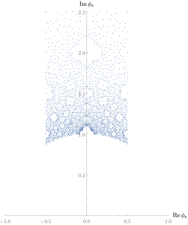
Figure 1: A sampling of vacua (7.25) filling the fundamental domain (7.22), for the values of the constants $e_{I},m^{J}\in[-11,11]$.

On the other hand, in order to identify the inequivalent vacua, corresponding to inequivalent choices of the constants (7.19) and of the corresponding effective potentials, we can restrict ourselves to the vacua (7.25) which sit in the fundamental domain of (7.22). The set of such vacua is plotted in Fig. 1. A similar set of vacua appears in the simplest models of type IIB flux compactifications on a rigid Calabi–Yau [81], in which $\phi$ can be identified with the axion-dilaton. In the type IIB models one needs to impose the tadpole cancellation condition, which adds a constraint on the set of allowed vacua. In our formulation with gauge three-forms, the tadpole cancellation condition can be implemented as outlined at the end of Section 3.3.

8 Domain walls between aligned vacua

In this section we explicitly construct a class of domain walls of the kind discussed in Section 6, relating pairs of vacua $\phi|_{-\infty}=\phi_{*}$ and $\phi|_{+\infty}=\phi_{*}^{\prime}$ of the form (7.25), corresponding to two sets of constants $\alpha_{I}$ and $\alpha_{I}^{\prime}$ respectively. We make the simplifying assumption that the phases of ${\cal Z}_{*}$ and ${\cal Z}^{\prime}_{*}$ are aligned and that the phase of ${\cal Z}(y)$ remains constant along the flow. Of course, in order to have a (non-trivial) domain wall $|{\cal Z}_{*}|$ and $|{\cal Z}^{\prime}_{*}|$ should be different and then the corresponding vacua cannot be related by a $SL(2,\mathbb{Z})$ duality. From (6.12) we see that we should impose ${\rm Im\hskip 1.00006pt}(\dot{\phi}\,\partial_{\phi}K)=0$ with $K$ as in (7.8). This is possible only if ${\rm Re\hskip 1.00006pt}\phi$ is constant and equals to

$${\rm Re\hskip 1.00006pt}\phi_{*}=-\frac{{\rm Im\hskip 1.00006pt}(\alpha_{0}\bar{\alpha}_{1})}{|\alpha_{1}|^{2}}.$$ (8.1)

Clearly, we should also require ${\rm Re\hskip 1.00006pt}\phi_{*}^{\prime}={\rm Re\hskip 1.00006pt}\phi_{*}$ . Hence,

$$v(y)\equiv{\rm Im\hskip 1.00006pt}\phi(y)$$ (8.2)

is the only dynamical real field along the flow. As in Section 6, we will assume that $|{\cal Z}|$ is always increasing along the flow, which drives the field $v$ from $v|_{-\infty}=v_{*}$ towards $v|_{+\infty}=v_{*}^{\prime}$ and, at $y=0$, it crosses a membrane of charges $p^{I},q_{J}$ such that

$$q_{0}-{\rm i}p^{1}=\alpha_{0}-\alpha_{0}^{\prime}\,,\quad q_{1}-{\rm i}p^{0}=\alpha_{1}-\alpha^{\prime}_{1}\,.$$ (8.3)

The equations of the flow (6.20) are governed by the growth of $|{\cal Z}|$. In particular, equation (6.20a) reduces to

$$\dot{v}=4v^{2}\,\frac{\text{d}}{\text{d}v}|{\cal Z}|\,.$$ (8.4)

For $y<0$, $|{\cal Z}|$ takes the following form

$$|{\cal Z}(v)|=\frac{e^{\frac{1}{2}\hat{K}_{0}}}{2\sqrt{v}}\left[|\alpha_{1}|v+\frac{{\rm Re\hskip 1.00006pt}(\alpha_{0}\bar{\alpha}_{1})}{|\alpha_{1}|}\right]\,.$$ (8.5)

For $y>0$ the from of $|{\cal Z}|$ is obtained by replacing $\alpha_{I}$ with $\alpha_{I}^{\prime}$ in (8.5).

On the left of the membrane, $v_{*}$ is a global minimum of $|{\cal Z}|$. Hence, it is a repulsive fixed point of (8.4), a flow is triggered and $v$ is driven away from $v_{*}$, letting the value of $|{\cal Z}|$ increase. When the membrane is reached at $y=0$, $v$ and consequently $|{\cal Z}|$ have evolved to certain values $v(0)$ and $|{\cal Z}|_{y=0}$. Here, the solution of the flow equations on the left should be glued to the one on the right. We are then led to impose the continuity of $v$ across $y=0$ while still keeping a growing $|{\cal Z}|$. However, since on the right of the membrane $v_{*}^{\prime}$ is also a global minimum of $|{\cal Z}|$, $v_{*}^{\prime}$ is a repulsive (rather than attractive) fixed point of (8.4). Hence the solution to the flow equations is such that $v$ reaches the value $v_{*}^{\prime}$ at $y=0$ and then remains constant

$$v(y)=v_{*}^{\prime}\quad\text{for}\;\,\,y\geq 0\,.$$ (8.6)

Correspondingly, $|{\cal Z}|$ starts from $|{\cal Z}_{*}|$ at $y=-\infty$ and smoothly grows until it reaches the membrane. At this point it jumps up to $|{\cal Z}^{\prime}_{*}|$ and then remains constant (see Fig. 4 for an example). Hence, on the right of the membrane, the background is just the AdS vacuum solution.

Recalling (6.36), we see that the bound

$$T_{\rm DW}\geq T_{\rm M}\,$$ (8.7)

is saturated if and only if on the left-hand side of the membrane $|{\cal Z}|$ is also constant. In the following we will first examine the case in which the bound (8.7) is saturated, leading to trivial flow equations on both sides of the membrane, and then we will consider an example for which the inequality (8.7) strictly holds.

As a warm up, let us assume that on the left of the membrane $\vec{\alpha}=0$, so that the potential (7.21) and ${\cal Z}$ are identically zero. Then, for $y<0$, the flow equations (6.20) are trivial and are immediately solved by taking $v$ and $D$ to be arbitrary constants. In particular, with no loss of generality, we can choose $D(y)\equiv 0$ for $y<0$. Therefore, on the left of the membrane, the bulk is always at a fixed Minkowski vacuum. As discussed above, on the right of the membrane, the bulk is at its supersymmetric AdS vacuum, in which $v$ takes the constant value $v_{*}^{\prime}$. Hence, by continuity, we should impose that $v(y)\equiv v_{*}^{\prime}$ also for $y<0$. Furthermore, by imposing also the continuity of the warp factor, we must set $D(y)=-|{\cal Z}^{\prime}_{*}|y$ for $y>0$.

It is worthwhile to mention that this particular case of trivial flow for both $y<0$ and $y>0$ can be realized only when on the left-hand side the vacuum is Minkowski, owing to the freedom in choosing any constant value of $v$ for $y<0$.

Let us now consider a more involved example, for which the flow on the left side of the membrane is nontrivial. For any choice of initial constants $\alpha_{0},\alpha_{1}$ and any $k\in\mathbb{Q}$ such that

$$k\alpha_{1}\in\mathbb{Z}+{\rm i}\mathbb{Z}$$ (8.8)

we can choose a jump to new constants

$$\alpha_{0}^{\prime}=\alpha_{0}+k\alpha_{1}\,,\quad\alpha_{1}^{\prime}=\alpha_{1}\,,$$ (8.9)

which clearly satisfies ${\rm Re\hskip 1.00006pt}\phi_{*}^{\prime}={\rm Re\hskip 1.00006pt}\phi_{*}$. Notice that

$${\rm Im\hskip 1.00006pt}\phi^{\prime}_{*}={\rm Im\hskip 1.00006pt}\phi_{*}+k\,.$$ (8.10)

The flow moves along the vertical direction of the upper-half-plane parametrized by $\phi$ (see Fig. 2). With no loss of generality, we take $k>0$, so that ${\rm Im\hskip 1.00006pt}\phi^{\prime}_{*}>{\rm Im\hskip 1.00006pt}\phi_{*}$. From (7.28), one can also see that $|{\cal Z}_{*}^{\prime}|>|{\cal Z}_{*}|$ which is the default assumption in Section 6.

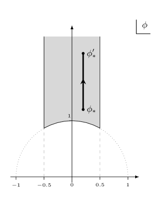
Figure 2: The fundamental domain of $\phi$. Along the domain wall, $\phi$ flows up along the vertical line specified by ${\rm Re\hskip 0.80005pt}\phi_{*}$.

Under these restrictions, the initial and final values of $v(y)$ are

$$v_{*}=\frac{{\rm Re\hskip 1.00006pt}(\alpha_{0}\bar{\alpha}_{1})}{|\alpha_{1}|^{2}}\,,\quad~{}~{}~{}~{}v_{*}^{\prime}=\frac{{\rm Re\hskip 1.00006pt}(\alpha_{0}\bar{\alpha}_{1})}{|\alpha_{1}|^{2}}+k$$ (8.11)

and the membranes charges are

$$p^{0}=0\,,\quad p^{1}=k\,{\rm Im\hskip 1.00006pt}\alpha_{1}\,,\quad q_{0}=-k\,{\rm Re\hskip 1.00006pt}\alpha_{1}\,,\quad q_{1}=0\,.$$ (8.12)

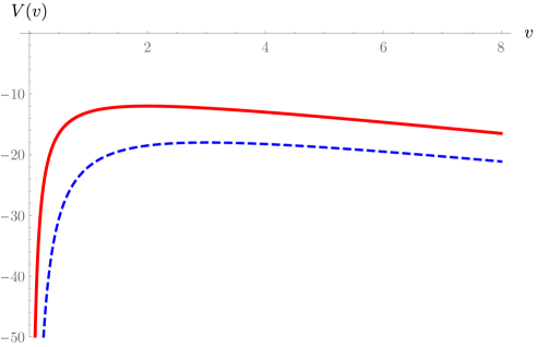
Figure 3: The potential (7.21) for the choice of the constants $e_{1}=m^{0}=1$, $e_{0}=m^{1}=2$, $k=1$ and keeping ${\rm Re\hskip 0.80005pt}\phi=0$. The solid red line refers to the potential on the left of the membrane, while the dashed blue line to that on the right. This potential exhibits, on the left of the membrane, a supersymmetric AdS critical point located at $v_{*}=2$ and, on the right, a supersymmetric AdS critical point at $v_{*}^{\prime}=3$.

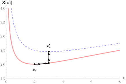
Figure 4: The flow of $|{\cal Z}|$ for the same set of parameters as in Fig. 3. The solid red line refers to $|{\cal Z}|$ on the left of the membrane, while the dashed blue line to that on the right. The flow drives $v_{*}$ towards the value $v_{*}^{\prime}$, at which $|{\cal Z}|$ jumps so that $v$ is located at new supersymmetric vacuum on the right.

We can now compute the function ${\cal Z}(v,y)$ corresponding to our setting

$${\cal Z}(v,y)=\frac{\bar{\alpha}_{1}e^{\frac{1}{2}\hat{K}_{0}}}{2|\alpha_{1}|\sqrt{v}}\left[|\alpha_{1}|v+\frac{{\rm Re\hskip 1.00006pt}(\alpha_{0}\bar{\alpha}_{1})}{|\alpha_{1}|}+k|\alpha_{1}|\Theta(y)\right].$$ (8.13)

In agreement with (6.21), ${\cal Z}(v,y)$ is discontinuous at $y=0$ and the width of the discontinuity is set by the tension of the membrane with the charges (8.12)

$$\lim_{\varepsilon\rightarrow 0}\Big{|}{\cal Z}(y_{\rm M}+\varepsilon)-{\cal Z}(y_{\rm M}-\varepsilon)\Big{|}=\frac{k|\alpha_{1}|e^{\frac{1}{2}\hat{K}_{0}}}{2\sqrt{v|_{y=0}}}\equiv\frac{1}{2}T_{M}.$$ (8.14)

An example for the flow of $|{\cal Z}|$ is depicted in Fig. 4.

Consider now the flow equation (8.4). For the examples under consideration, it takes the explicit form

$$\dot{v}=e^{\frac{1}{2}\hat{K}_{0}}\sqrt{v}\left[|\alpha_{1}|v-\frac{{\rm Re\hskip 1.00006pt}(\alpha_{0}\bar{\alpha}_{1})}{|\alpha_{1}|}-k|\alpha_{1}|\Theta(y)\right]\,,$$ (8.15)

which is solved by

$$v(y)=\left\{\begin{array}[]{l}v_{*}\coth^{2}\left[\frac{1}{2}|{\cal Z}_{*}|(y+c)\right]\quad~{}~{}\text{for $y\leq 0$}\,,\\ v_{*}^{\prime}\quad~{}~{}~{}~{}~{}~{}~{}~{}~{}~{}~{}~{}~{}~{}~{}~{}~{}~{}~{}~{}~{}~{}~{}~{}~{}~{}~{}~{}~{}\text{for $y\geq 0$}\,.\end{array}\right.\,$$ (8.16)

The integration constant $c$ must be negative, $c<0$, and is fixed by the continuity at $y=0$, which imposes $v_{*}\coth^{2}\left[\frac{1}{2}c\,|{\cal Z}_{*}|\right]=v_{*}^{\prime}$ and always admits a solution.

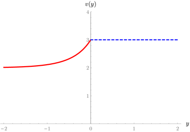
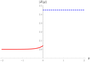
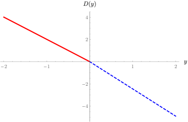
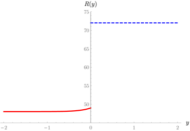
Figure 5: Above are depicted all the solutions to the flow equations (8.15), (8.18) for the same set of parameters as in Fig. 3. The solid red lines refer to the quantities in the region on the left of the membrane, while the dashed blue lines to those on the right. On the top left there is the evolution of the scalar field: starting from the critical point on the left of the membrane, the field $v$ is driven towards the critical point on the right of the membrane. On the top right there is the modulus of the covariantly holomorphic superpotential $|{\cal Z}|$, which is always increasing. On the bottom left there is the warping $D(y)$, which is always decreasing, using which the curvature, on the bottom right, can be obtained. As expected from the AdS vacua, the curvature is at a fixed positive value when the field $v$ reaches the vacua and, even though not explicitly shown here, is singular at the point $y=0$. In the figures $y$ is $|{\cal Z}_{*}|^{-1}$ units.

Since the bulk exhibits a non-trivial flow only on the left-hand side of the membrane, the membrane tension is given by the vacuum expectation value of $\phi_{*}^{\prime}$ to the right of the membrane

$$T_{\rm M}=\frac{k|\alpha_{1}|^{2}e^{\hat{K}_{0}}}{|{\cal Z}^{\prime}_{*}|}.$$ (8.17)

We still have to solve the equation for the warping (6.20b), which in the present case reads

$$\dot{D}=-\frac{e^{\frac{1}{2}\hat{K}_{0}}}{2\sqrt{v}}\left[|\alpha_{1}|v+\frac{{\rm Re\hskip 1.00006pt}(\alpha_{0}\bar{\alpha}_{1})}{|\alpha_{1}|}+k|\alpha_{1}|\Theta(y)\right].$$ (8.18)

It also admits an analytic solution given by

$$D(y)=\left\{\begin{array}[]{l}d+{e^{-\frac{1}{2}\hat{K}_{0}}\left(\log(-\sinh u)+\log\cosh u\right)}\quad~{}\text{for $y\leq 0$}\,,\\ -|{\cal Z}_{*}^{\prime}|y\quad~{}~{}~{}~{}~{}~{}~{}~{}~{}~{}~{}~{}~{}~{}~{}~{}~{}~{}~{}~{}~{}~{}~{}~{}~{}~{}~{}~{}~{}~{}~{}~{}~{}~{}~{}~{}~{}~{}~{}~{}~{}\text{for $y\geq 0$}\,,\end{array}\right.$$ (8.19)

where we have set to zero an arbitrary additive constant and $u(y)\equiv\frac{1}{2}|{\cal Z}_{*}|(y+c)$. The integration constant $d$ is fixed by imposing the continuity of $D(y)$ at $y=0$.

A couple of final comments. Notice that on the left-hand side of the membrane the deviation of the complete solution from the AdS vacuum is concentrated within a length of the same order of the AdS radius $|{\cal Z}_{*}|^{-1}$. Hence, in this sense, the domain wall may be considered as ‘thick’. Furthermore, clearly, we can make a coordinate redefinition $y\rightarrow y-y_{\rm M}$ to get a solution with the membrane localised at any point $y_{\rm M}$.

9 Conclusions

In this paper we have studied and expanded the ${\cal N}=1$ supergravities including double three-form multiplets introduced in [28]. We have focused on the subclass of models in which the dynamics of the double three-form multiplet sector is governed by a special Kähler structure and is covariant under symplectic tranformations.

Into this setup we have included supermembranes of arbirary (quantised) charges, which naturally couple to the supersymmetric completion of the three-form potentials via a WZ term. Given the WZ term, the worldvolume $\kappa$-symmetry of the membrane action fixes the form of its NG term which includes the dependence on the bulk scalar sector in the way expected from string compactification models (see Appendix D for the proof of $\kappa$-symmetry and Appendix E for further generalizations).

The back-reaction of the membrane induces a jump in the vevs of the four-form field-strengths. Hence, from a more conventional supergravity perspective (which can be retrieved from the three-form theory by setting the field-strengths on-shell), this implies the appearance of an effective superpotential with different coupling constants on the left and on the right-hand side of the membrane. Within this setup we have examined how supersymmetric vacua corresponding to different four-form flux integration constants separated by the membrane are connected by ‘jumping’ BPS domain walls. As a simple and instructive example we have considered a model with two double three-form multiplets and found explicit analytic solutions describing jumping domain walls therein. Thus, our results generalize the class of the BPS domain walls of four-dimensional $\mathcal{N}=1$ supergravities studied previously e.g. in [39, 40, 41, 42, 43, 8, 44, 33].

We believe that the results of this paper provide an appropriate starting point for describing, from an effective four-dimensional perspective, non-trivial dynamical processes involving at the same time membranes, fluxes and the scalar sector of flux compactifications, as for instance those considered in [9, 10]. In particular, in this paper we have only considered the effects of membranes on flat BPS domain walls, postponing the study of other possible dynamical effects (for example, the nucleation of non-BPS membrane bubbles) and their physical implications to the future.

Acknowledgements

We thank G. Dall’Agata, I. Garcίa-Etxebarria, S. Kuzenko and I. Valenzuela for useful discussions. Work of I.B. was supported in part by the Spanish MINECO/FEDER (ERDF) EU grant FPA 2015-66793-P, by the Basque Government Grant IT-979-16, and the Basque Country University program UFI 11/55. Work of F.F. is supported in part by the Interuniversity Attraction Poles Programme initiated by the Belgian Science Policy (P7/37), and in part by support from the KU Leuven C1 grant ZKD1118 C16/16/005. Work of S.L. and L.M. was partially supported by the Padua University Project CPDA144437. Work of D.S. was supported in part by the Russian Science Foundation grant 14-42-00047 in association with Lebedev Physical Institute and by the Australian Research Council project No. DP160103633. D.S. is grateful to the Department of Physics, UWA and the School of Mathematics, the University of Melbourne for hospitality at an intermediate stage of this project.

Appendix A Super-Weyl transformations

The Lagrangian (2.1) is invariant under the super-Weyl transformations of the chiral superfields and the super-vielbein [51, 52]

$$Z \rightarrow e^{-6\Upsilon}Z,$$ (A.1)

$$E^{a}_{M} \rightarrow e^{\Upsilon+\bar{\Upsilon}}E^{a}_{M},$$

$$E^{\alpha}_{M} \rightarrow e^{2\Upsilon-\bar{\Upsilon}}\left(E^{\alpha}_{M}-\frac{{\rm i}}{2}E_{M}^{\alpha}\sigma_{a}^{\alpha\dot{\alpha}}\bar{\cal D}_{\dot{\alpha}}\bar{\Upsilon}\right).$$

After singling out the chiral compensator as in (3.4), we can think of the super-Weyl transformation as acting on the chiral compensator only

$$Y\rightarrow e^{-6\Upsilon}Y$$ (A.2)

leaving the chiral superfields $\Phi^{i}$ invariant. Under a general Kähler transformation

$$K(\Phi,\bar{\Phi})\rightarrow K(\Phi,\bar{\Phi})+f(\Phi)+\bar{f}(\bar{\Phi})$$ (A.3)

the Lagrangian (2.1) is not invariant. Such invariance is only restored if (A.3) is accompanied by a super-Weyl rescaling of the compensator and the superpotential, namely

$$Y \rightarrow e^{-f(\Phi)}Y\,,$$ (A.4)

$$W(\Phi) \rightarrow e^{-f(\Phi)}W(\Phi)\,.$$

In other words, the chiral compensator and the superpotential are holomorphic sections of a complex line bundle over the Kähler manifold.

The prepotential $\mathcal{P}$ which determines the structure of the three-form gauge superfield $\mathcal{A}_{3}$ in (5.4) transforms under the Weyl rescaling as follows

$$\mathcal{P}\to e^{-2(\Upsilon+\bar{\Upsilon})}\mathcal{P}.$$ (A.5)

This ensures that $\mathcal{A}_{3}$ is Weyl invariant [34].

Appendix B General bosonic action

With the choice of the kinetic function as in (3.1) and (3.2), the most general superfield action built from (2.8) leads to the bosonic component action of the following form

$$S_{\rm bos}= -\int\text{d}^{4}x\,e\,\Big{(}\frac{1}{2}R+G_{IJ}f^{I}{}_{i}\bar{f}^{J}{}_{\bar{\jmath}}\;\partial\phi^{i}\partial\bar{\phi}^{\bar{\jmath}}+\hat{K}_{p\bar{q}}\,\partial t^{p}\partial\bar{t}^{\bar{q}}\Big{)}$$ (B.1)

$$+S_{\text{3-forms}}+S_{\hat{W}}\,$$

where the three-form action $S_{\text{3-forms}}$ is

$$S_{\text{3-forms}}=\int\text{d}^{4}x\,e\,{\cal T}^{IJ}{}^{*}\!\bar{\cal F}_{4I}\,{}^{*}{}\!{\cal F}_{4J}+S_{\rm 3-forms,\,bd}$$ (B.2)

and the $\hat{W}$-depending action $S_{\rm\hat{W}}$ is (where we use the property of the superpotential $\hat{W}=\hat{W}_{K}f^{K}$)

$$S_{\hat{W}}= \int\text{d}^{4}x\,e\,\left\{-\text{e}^{\cal K}\left[\hat{K}^{\bar{q}p}-\frac{1}{\gamma}\hat{K}^{\bar{q}l}\hat{K}_{l}\hat{K}^{\bar{l}p}\hat{K}_{\bar{l}}\right]\hat{W}_{p}\overline{\hat{W}}_{\bar{q}}\right\}$$ (B.3)

$$+{\rm Re\hskip 1.00006pt}\int\text{d}^{4}x\,e\,\Bigg{\{}-\frac{{\rm i}}{\gamma(f{\cal M}\bar{f})}\hat{K}_{\bar{q}}\hat{K}^{\bar{q}p}\hat{W}_{p}\bar{f}^{I}{}^{*}{}\!{\cal F}_{4I}+$$

$$+{\rm i}(f{\cal M}\bar{f})\left[\hat{W}_{K}G_{IL}{\cal M}^{LK}{\cal M}^{IN}-\frac{\hat{W}\bar{f}^{N}}{(f{\cal M}\bar{f})^{2}}\right]\,{}^{*}{}\!{\cal F}_{4N}\Bigg{\}}+S_{\hat{W},\,\rm bd}\,.$$

Here $\gamma$ is defined as in (3.16c). The boundary terms are given by

$$S_{\rm 3-forms,\,bd} =\,2{\rm Re\hskip 1.00006pt}\int_{\cal B}{\cal T}^{IJ}(\tilde{A}_{3I}-{\cal G}_{IK}A_{3}^{K}){}^{*}\!{\cal F}_{4J}\,$$ (B.4)

and

$$S_{\hat{W},\,\rm bd}= \,{\rm Re\hskip 1.00006pt}\int_{{\cal B}}\Bigg{\{}-\frac{{\rm i}}{\gamma(f{\cal M}\bar{f})}\hat{K}_{\bar{q}}\hat{K}^{\bar{q}p}\hat{W}_{p}\bar{f}^{I}(\tilde{A}_{3I}-{\cal G}_{IK}A_{3}^{K})+$$ (B.5)

$$+{\rm i}(f{\cal M}\bar{f})\left[\hat{W}_{K}G_{IL}{\cal M}^{LK}{\cal M}^{IN}-\frac{\hat{W}\bar{f}^{N}}{(f{\cal M}\bar{f})^{2}}\right](\tilde{A}_{3N}-{\cal G}_{NP}A_{3}^{P})\Bigg{\}}\,.$$

Appendix C Supersymmetry transformations of fermions

In the double three-form supergravity under consideration the supersymmetry transformations of the gravitino and the chiralini, in the bosonic background, have the following form

$$\delta\psi_{m}{}^{\alpha} =-2\hat{{\cal D}}_{m}\zeta^{\alpha}-{\rm i}e_{m}{}^{c}e^{-\frac{{\cal K}}{2}}W(\epsilon\sigma_{c}\bar{\zeta})^{\alpha}\,,$$ (C.1)

$$\delta\chi^{i}_{\alpha} =\sqrt{2}\zeta_{\alpha}e^{\frac{{\cal K}}{2}}K^{\bar{\jmath}i}(\overline{W}_{\bar{\jmath}}+K_{\bar{\jmath}}\overline{W})-{\rm i}\sqrt{2}\sigma_{\alpha\dot{\beta}}{}^{a}\bar{\zeta}^{\dot{\beta}}\partial_{a}\phi^{i}\,,$$

$$\delta\rho^{p}_{\alpha} =\sqrt{2}\zeta_{\alpha}e^{\frac{{\cal K}}{2}}\hat{K}^{\bar{q}p}K_{\bar{q}}\overline{W}-{\rm i}\sqrt{2}\sigma_{\alpha\dot{\beta}}{}^{a}\bar{\zeta}^{\dot{\beta}}\partial_{a}t^{p}\,,$$

where $W$ and $W_{i}$ were defined in (3.23), the covariant derivative of the supersymmetry parameter is given by

$$\begin{split}\hat{{\cal D}}_{m}\zeta^{\alpha}&\equiv\partial_{m}\zeta^{\alpha}+\zeta^{\beta}\omega_{m\beta}{}^{\alpha}-\frac{{\rm i}}{2}{\cal A}_{m}\zeta^{\alpha}\,,\end{split}$$ (C.2)

and the $U(1)$ Kähler connection is

$${\cal A}_{m}=\frac{{\rm i}}{2}\left(K_{i}\partial_{m}\phi^{i}-K_{{\overline{\imath}}}\partial_{m}\bar{\phi}^{\overline{\imath}}+\hat{K}_{p}\partial_{m}t^{p}-\hat{K}_{\bar{p}}\partial_{m}\bar{t}^{\bar{p}}\right)\,.$$ (C.3)

In the absence of $T_{p}$ multiplets, the BPS condition on the domain wall ansatz discussed in Section 6 is obtained by setting to zero the corresponding variations (C.1), which reduce to

$$\delta\psi_{y}{}^{\alpha}= -2\dot{\zeta}^{\alpha}+{\rm i}{\cal A}_{y}\zeta^{\alpha}-{\rm i}e^{\frac{{\cal K}}{2}}W(\epsilon\sigma_{\underline{y}}\bar{\zeta})^{\alpha}\,,$$ (C.4)

$$\delta\psi_{i}{}^{\alpha}= e^{D}\left[\dot{D}\ (\zeta\sigma_{\underline{y}}\bar{\sigma}_{\underline{i}})^{\alpha}-{\rm i}e^{\frac{{\cal K}}{2}}W(\epsilon\sigma_{\underline{i}}\bar{\zeta})^{\alpha}\right]\,,$$

$$\delta\chi^{i}_{\alpha}= \sqrt{2}\zeta_{\alpha}e^{\frac{{\cal K}}{2}}K^{\bar{\jmath}i}(\overline{W}_{\bar{\jmath}}+K_{\bar{\jmath}}\overline{W})-{\rm i}\sqrt{2}\sigma_{\alpha\dot{\beta}}{}^{\underline{y}}\bar{\zeta}^{\dot{\beta}}\dot{\phi}^{i}\,.$$

Appendix D Proof of $\kappa$-symmetry

In superspace, we mostly follow notation and conventions of [82]. In particular, for the superspace superform algebra of this and the following appendices, we adopt the inverse-index notation and the external-derivative acts from the right.

The action of the supermembrane in the background of supergravity and three-form multiplets, (5.11), (5.9) and (5.2), can be written in the following form

$$S_{M}=S_{NG}+S_{WZ}=-2\int_{{\cal C}}\text{d}^{3}\xi\sqrt{-\det\,h}\;|T|+\int_{{\cal C}}{\cal A}_{3}\;,\qquad$$ (D.1)

where $T$ is a composite special chiral superfield

$$T=q_{I}S^{I}-p^{I}{\cal G}_{I}(S)=q_{I}S^{I}-p^{I}{\cal G}_{IJ}(S)S^{J}\,,$$ (D.2)

which is constructed as

$$T=-\frac{{\rm i}}{4}(\bar{{{\cal D}}}^{2}-8{\cal R})\cal P$$ (D.3)

from the composite prepotential

$${\cal P}=q_{I}{\cal P}^{I}-p^{I}\tilde{{\cal P}}_{I}=-2q_{I}{\cal M}^{IJ}{\rm Im\hskip 1.00006pt}\Sigma_{J}+2p^{I}{\rm Im\hskip 1.00006pt}(\bar{\cal G}_{IJ}{\cal M}^{JK}\Sigma_{K})$$ (D.4)

in which ${\cal P}^{I}$ and $\tilde{{\cal P}}_{I}$ were defined in (4.9). The three-form ${\cal A}_{3}$ in the WZ term of (D.1) is constructed as in (5.4) with the composite prepotential (D.4). The field strength of this super-three-form is

$${\cal H}_{4} = \text{d}{\cal A}_{3}=\;{{\rm i}}E^{b}\wedge E^{a}\wedge\bar{E}^{\dot{\alpha}}\wedge\bar{E}^{\dot{\beta}}\bar{\sigma}_{ab\;\dot{\alpha}\dot{\beta}}T-{{\rm i}}E^{b}\wedge E^{a}\wedge E^{\alpha}\wedge E^{\beta}\sigma_{ab\;\alpha\beta}\bar{T}\qquad$$ (D.5)

$$-\frac{{\rm i}}{6}E^{c}\wedge E^{b}\wedge E^{a}\wedge\bar{E}^{\dot{\alpha}}\epsilon_{abcd}\sigma^{d}_{\alpha\dot{\alpha}}{\cal D}^{\alpha}{T}-\frac{{\rm i}}{6}E^{c}\wedge E^{b}\wedge E^{a}\wedge E^{\alpha}\epsilon_{abcd}\sigma^{d}_{\alpha\dot{\alpha}}\bar{{\cal D}}^{\dot{\alpha}}\bar{T}$$

$$+\frac{1}{96}E^{d}\wedge E^{c}\wedge E^{b}\wedge E^{a}\epsilon_{abcd}\left(({\cal D}{\cal D}-24\bar{{\cal R}}){T}+(\bar{{\cal D}}\bar{{\cal D}}-24{\cal R})\bar{T}\right)\,.\qquad$$

The measure $\text{d}^{3}\xi$ in the Nambu-Goto type term is defined by

$$\text{d}\xi^{i}\wedge\text{d}\xi^{j}\wedge\text{d}\xi^{k}=\epsilon^{ijk}\,\text{d}^{3}\xi\;.$$ (D.6)

This implies the identities

$$\text{d}^{3}\xi\sqrt{-h}=\frac{1}{3}{}^{*_{3}}\!E_{a}\wedge E^{a}\;,\qquad\text{d}^{3}\xi\,\delta\sqrt{-h}={}^{*_{3}}\!E_{a}\wedge\delta E^{a}\;,\qquad$$ (D.7)

where the action of worldvolume Hodge duality operation ${}^{*_{3}}$ on a one-form is defined by

$${}^{*_{3}}\!E^{A}:=\frac{1}{2}\text{d}\xi^{j}\wedge\text{d}\xi^{i}\sqrt{-h}\epsilon_{ijk}h^{kl}E_{l}^{A}\;.\qquad$$ (D.8)

This latter can be used to write the variation of the Nambu-Goto action with respect to the embedding coordinates $z^{M}(\xi)$ in the form

$$\delta S_{NG}=-2\int_{{\cal C}}{}^{*_{3}}\!E_{a}\wedge\delta E^{a}\,|T|-2\int_{{\cal C}}\text{d}^{3}\xi\sqrt{-h}\frac{T\delta\bar{T}+\delta T\,\bar{T}}{|T|}\;,\qquad$$ (D.9)

while the variation of the Wess-Zumino term is

$$\delta S_{WZ}=\int_{{\cal C}}\delta{\cal A}_{3}=\int_{{\cal C}}(i_{\delta z}\text{d}{\cal A}_{3}+\text{d}\,i_{\delta z}{\cal A}_{3})=\int_{{\cal C}}i_{\delta z}{\cal H}_{4}.$$ (D.10)

Here for varying ${{\cal C}}$ we used the Lie derivative formula $\delta_{z}=\text{d}i_{\delta z}+i_{\delta_{z}}\text{d}$ and its Lorentz covariant extension

$$\delta_{z}={\cal D}i_{\delta z}+i_{\delta z}{\cal D}\,,$$ (D.11)

which is equivalent to the Lie derivative modulo local Lorentz transformations.

We are searching for $\kappa$-symmetry transformations, leaving the supermembrane action invariant, in the form which is common for a general class of superbranes, i.e.

$$\begin{split}&i_{\kappa}E^{a}=\delta_{\kappa}z^{M}E_{M}^{a}(z)=0\;,\qquad\\ &i_{\kappa}E^{\alpha}=\delta_{\kappa}z^{M}E_{M}^{\alpha}(z)=\kappa^{\alpha}\;,\qquad i_{\kappa}E^{\dot{\alpha}}=\delta_{\kappa}z^{M}E_{M}^{\dot{\alpha}}(z)=\bar{\kappa}{}^{\dot{\alpha}}\;.\qquad\end{split}$$ (D.12)

For this transformations the variations of the bosonic supervielbein, chiral superfields and the WZ term take the form

$$\delta_{\kappa}E^{a}={\cal D}i_{\kappa}E^{a}+i_{\kappa}{\cal D}E^{a}=-2{\rm i}E^{\alpha}(\sigma^{a}\bar{\kappa})_{\alpha}+2{\rm i}({\kappa}\sigma^{a})_{\dot{\alpha}}E^{\dot{\alpha}}\;,$$ (D.13)

$$\delta_{\kappa}T=\kappa^{\alpha}{\cal D}_{\alpha}T\;,\qquad\delta_{\kappa}\bar{T}=\kappa^{\alpha}\bar{{\cal D}}_{\dot{\alpha}}\bar{T}\,,$$ (D.14)

$$\begin{split}i_{\kappa}{\cal H}_{4}=\;&-2{\rm i}E^{b}\wedge E^{a}\wedge\bar{E}^{\dot{\alpha}}(\bar{\kappa}\bar{\sigma}_{ab})_{\dot{\alpha}}T+2{\rm i}E^{b}\wedge E^{a}\wedge E^{\alpha}(\sigma_{ab}\kappa)_{\alpha}\bar{T}-\\ &-\frac{{\rm i}}{6}E^{c}\wedge E^{b}\wedge E^{a}\epsilon_{abcd}(\sigma^{d}\bar{\kappa})_{\alpha}{\cal D}^{\alpha}{T}-\frac{{\rm i}}{6}E^{c}\wedge E^{b}\wedge E^{a}\epsilon_{abcd}(\kappa\sigma^{d})_{\dot{\alpha}}\bar{{\cal D}}^{\dot{\alpha}}\bar{T}\;.\end{split}$$ (D.15)

Now, using the identities

$$E^{b}\wedge E^{c}\wedge E^{\beta}\sigma_{bc\,\beta}{}^{\alpha}=-2\,{}^{*_{3}}\!E^{a}\wedge E^{\beta}(\sigma_{a}\,{\Gamma})_{\beta}{}^{\alpha}\;,$$ (D.16)

$$\text{d}^{3}\xi\sqrt{-h}{\Gamma}=\frac{{\rm i}}{3!}\sigma^{a}\epsilon_{abcd}E^{b}\wedge E^{c}\wedge E^{d}\,,$$

one can check that the variation of the WZ term (D.10) cancel the variation (D.9) of the NG term, provided

$$\kappa_{\alpha}=\frac{T}{|T|}({\Gamma}\bar{\kappa})_{\alpha}\;.$$ (D.17)

This is exactly the condition (5.13) of the main text.

Appendix E Generic systems of 3-form matter, supergravity and supermembranes

The supermembrane interaction with a single three-form multiplet is described by the equations from the previous section, if we consider the special chiral superfield $T$ to be fundamental, i.e. expressed through a single fundamental real prepotential ${\cal P}$ rather than composite as in (D.2). In this case the chiral superfield $T$ has the auxiliary field $F_{T}=F+{\rm i}{}^{*}\!F_{4}$ whose real part is a scalar and the imaginary part is the dual of the single four-form.

Now, to describe general systems of supergravity and three-forms coupled to the membrane we introduce a set of chiral superfields of conformal weight 3, $Z^{\Lambda}$ ($\Lambda=(\mathfrak{I},I)$), where the indices $\mathfrak{I}$ and $I$ label the subsets of double and single three-form superfields. In this set the conformal compensator $Y$ can be chosen at will. It can be either single- or double three-form superfield. Then the other superfields are associated with the double or single 3-form matter supermultiplets. Note that there also is a third case in which the conformal compensator is not among the independent fields of the set $Z^{\Lambda}$ coupled to the membrane. Then the supermembrane couples to supergravity only via the physical three-form superfields. In this case the off-shell supergravity can be consistently chosen to be the conventional old-minimal supergravity with the both components of its complex auxiliary field being scalars (and not three-forms).

The general action for the supermebrane coupled to the superfields $Z^{\Lambda}$ has the following form

$$S_{p=2}=-2\int_{{\cal C}}\text{d}^{3}\xi\sqrt{{-}h}|q_{\Lambda}{Z}^{\Lambda}|+q_{\mathfrak{I}}\int_{{\cal C}}{C}_{3}{}^{\mathfrak{I}}+\bar{q}_{\mathfrak{I}}\int_{{\cal C}}{\bar{C}}{}_{3}^{\mathfrak{I}}+q_{I}\int_{{\cal C}}{A}{}_{3}^{I}\;,\qquad$$ (E.1)

where $C_{3}^{\mathfrak{I}}$ are the complex super three-forms associated with the double three-form supermultiplets and the real super three-forms $A_{3}^{I}$ are associated with the single three-form ones.

The action is invariant under the kappa-symmetry transformations (D.13) and (D.17) in which $T={{q}_{\Lambda}{Z}^{\Lambda}}$.

Appendix F Membrane equations of motion

Here we enlist the equations of motion coming from the complete action (3.14)+(5.15) and their form after employing the domain wall ansatz (6.5).

First, the equation of motion of the graviton is

$$R^{mn}-{\frac{1}{2}}g^{mn}R=T^{mn}+g^{mn}V+\int\,\text{d}^{3}\xi\,T_{M}\frac{\sqrt{-h}}{\sqrt{-g}}\delta\left(x^{m}-z^{m}(\xi)\right)h^{ab}\partial_{a}z^{m}\partial_{b}z^{n}$$ (F.1)

with

$$T^{mn} =K_{i\bar{\jmath}}\left(g^{mn}g^{pq}-2g^{mp}g^{nq}\right)\partial_{p}\phi^{i}\partial_{q}\bar{\phi}^{j}.$$ (F.2)

Taking the trace of (F.1), we get the following equation for the scalar curvature

$$-\frac{R}{2}=K_{i\bar{\jmath}}\,\partial^{m}\phi^{i}\partial_{m}\bar{\phi}^{j}+2V+\frac{3}{2}\int\text{d}^{3}\xi\,\frac{\sqrt{-h}}{\sqrt{-g}}\delta\left(x^{m}-z^{m}(\xi)\right)T_{M}.$$ (F.3)

In the static gauge $x^{\mu}(\xi)=\xi^{i}\delta_{i}^{\mu}$, in which the only nontrivial worldvolume bosonic field is $y(x)$, the last term in (F.3) reduces to $\frac{3}{2}T_{M}\frac{\sqrt{-h}}{\sqrt{-g}}\delta\left(y-y(x)\right)$ and the equation for the scalar curvature becomes

$$-\frac{R}{2}=K_{i\bar{\jmath}}\,\partial^{m}\phi^{i}\partial_{m}\bar{\phi}^{j}+2{\cal T}^{IJ}{}^{*}\!\bar{\cal F}_{4I}\,{}^{*}\!{\cal F}_{4J}+\frac{3}{2}\frac{\sqrt{-h}}{\sqrt{-g}}\delta\left(y-y(x)\right)T_{M}.$$ (F.4)

The domain wall ansatz (6.5) implies that the only nonvanishing (vielbein) component of the spin connection is

$$\omega_{i}^{a3}=-\delta_{i}^{a}e^{2D(y)}\dot{D}\,,$$ (F.5)

so that the curvature two-form reduces to

$$R^{ab}=-e^{a}\wedge e^{b}\dot{D}^{2}+2\delta_{3}^{[a}e^{b]}\wedge dy\,\ddot{D}\;$$ (F.6)

and the Ricci scalar is

$$R=6\left(2\dot{D}^{2}+\ddot{D}\right)\;.$$ (F.7)

We can then combine (F.3) with the flow equation (6.20b), immediately getting

$$\frac{\text{d}|{\cal Z}|}{\text{d}y}=K_{i\bar{\jmath}}\dot{\phi}^{i}\dot{\bar{\phi}}^{\bar{\jmath}}+\frac{1}{2}T_{\rm M}\,\delta(y)$$ (F.8)

coherently with (6.21). The above equation is also implied by the three-form field equations (6.2) if one uses the definition of $W$ in (3.23). This shows the consistency of the supergravity equations of motion with the domain wall ansatz [8] and the flow equations [33].

Let us now come to the equations of motion for the membrane. When all the fermions are set to zero, in the Einstein frame the supermembrane action has the form (5.15), which we write as

$$S_{M}=-2\int\limits_{{\cal C}}d^{3}\xi\sqrt{-h}T_{M}+q^{I}\int\limits_{{\cal C}}A_{3}^{I}-p^{I}\int\limits_{{\cal C}}\tilde{A}_{3I}$$ (F.9)

with

$$T_{M}={\cal Z}=e^{\frac{1}{2}{\cal K}}|(q_{I}f^{I}(\phi)-p^{I}{\cal G}_{I}(\phi))|\,.$$ (F.10)

The supermembrane equations are then

$${\cal D}_{i}\left(\sqrt{-h}h^{ij}E_{ja}T_{M}\right)=\sqrt{-h}\,{\cal D}_{a}T_{M}+\frac{1}{3!}\varepsilon_{abcd}\varepsilon^{ijk}E_{i}^{b}E_{j}^{c}E_{k}^{d}\left(q_{I}{}^{*}\!F^{I}_{4}-p^{I}\!{}^{*}\tilde{F}_{I4}\right)\;,$$ (F.11)

where $E_{i}^{a}$ are coefficients of the pull back of the bosonic vielbein, $E_{i}^{a}=\partial_{i}x^{m}e_{m}^{a}(x(\xi))$. In the bosonic background (6.5), after fixing the ‘static gauge’ $x^{\mu}=\xi^{i}\delta_{i}^{\mu}$, these latter acquire the form

$$E_{i}^{a}=\partial_{i}y(x)\delta_{3}^{a}+e^{D(y)}\delta_{i}^{a}$$ (F.12)

so that

$$\begin{split}h_{ij}&=e^{2D(y)}\eta_{ij}+\partial_{i}y(x)\partial_{j}y(x)\;,\\ h^{ij}&=e^{-2D(y)}\left(\eta_{ij}-\frac{e^{-2D(y)}\partial^{i}y(x)\partial^{j}y(x)}{1+e^{-2D(y)}\partial^{k}y(x)\partial_{k}y(x)}\,\right)\;,\end{split}$$ (F.13)

where $\partial^{i}y(x)=\eta^{ij}\partial_{j}y(x)$. Let us consider a ground state solution of these equations in the domain wall background (6.5) in which the scalar fields depend only on the transverse coordinate $y$, $T_{M}=T_{M}(y)$, the three-form gauge potentials have the form (6.8), while

$${}^{*}\!F_{4}^{I}=-e^{-3D}\frac{\text{d}}{\text{d}y}\alpha^{I}(y)\;,\qquad{}^{*}\!\tilde{F}_{4I}=-e^{-3D}\frac{\text{d}}{\text{d}y}\tilde{\alpha}_{I}(y)\;,$$ (F.14)

and ${\cal D}_{a}T_{M}=\delta_{a}^{3}\frac{\text{d}}{\text{d}y}T_{M}$.

It is natural to assume that the ground state solution describes a flat membrane worldvolume such that

$$\partial_{i}y=0\quad\Rightarrow\qquad y(x)=y_{0}={\rm const}\;,$$

where $y_{0}$ indicates the place of the membrane in the bulk.

This implies that $E_{i}^{a}=e^{D(y_{0})}\delta_{i}^{a}$, $h_{ij}=e^{2D(y_{0})}\eta_{ij}$, ${\cal D}_{i}\left(\sqrt{-h}h^{ij}E_{ja}T_{M}\right)=-3\delta_{a}^{3}\dot{D}e^{D}T_{M}(y_{0})$, and the only nontrivial ($a=3$) component of the equations (F.11) takes the form

$$\left.\left(3\dot{D}T_{M}+\frac{\text{d}}{\text{d}y}T_{M}-q_{I}{}^{*}\!F^{4}_{I}(y)+p^{I}{}^{*}\!\tilde{F}_{4I}(y)\right)\right|_{y=y_{0}}=0\,,$$ (F.15)

or, taking into account (F.14), we have

$${}\left.\frac{\text{d}}{\text{d}y}\left(e^{3D}T_{M}+q_{I}\alpha^{I}-p^{I}\tilde{\alpha}_{I}\right)\right|_{y=y_{0}}=0\;,$$ (F.16)

where $T(y_{0})=T_{M}$ is the membrane tension.

Let us now connect the previous discussion with that of Section 6. There, we considered the (super)membrane action (5.15) as part of the action for the interacting system including dynamical supergravity and matter fields. In general, actions of this kind possess the bulk diffeomorphism invariance which can be used to choose, directly in the action, the gauge in which the embedding of the supermembrane worldvolume into the bulk is described by the equation

$$y(x)=0\,,$$ (F.17)

so that the transverse fluctuations of the membrane look ‘frozen’. Nevertheless, the supermembrane equations can still be obtained from the action in this gauge. They appear as self-consistency conditions of the supergravity (and matter) field equations (see [68, 70] and [80] for discussion and more references). A particular manifestation of this effect is that the membrane equations (6.40) are satisfied identically due to the consequence (6.41) of the flow equations (6.9).

References

- [1] M. J. Duff and P. van Nieuwenhuizen, Quantum Inequivalence of Different Field Representations, Phys. Lett. B94 (1980) 179–182.
- [2] A. Aurilia, H. Nicolai, and P. K. Townsend, Hidden Constants: The Theta Parameter of QCD and the Cosmological Constant of N=8 Supergravity, Nucl. Phys. B176 (1980) 509–522.
- [3] S. W. Hawking, The Cosmological Constant Is Probably Zero, Phys. Lett. B134 (1984) 403.
- [4] J. D. Brown and C. Teitelboim, Dynamical Neutralization of the Cosmological Constant, Phys. Lett. B195 (1987) 177–182.
- [5] J. D. Brown and C. Teitelboim, Neutralization of the Cosmological Constant by Membrane Creation, Nucl. Phys. B297 (1988) 787–836.
- [6] M. J. Duff, The Cosmological Constant Is Possibly Zero, but the Proof Is Probably Wrong, Phys. Lett. B226 (1989) 36. [Conf. Proc.C8903131,403(1989)].
- [7] M. J. Duncan and L. G. Jensen, Four Forms and the Vanishing of the Cosmological Constant, Nucl. Phys. B336 (1990) 100–114.
- [8] B. A. Ovrut and D. Waldram, Membranes and three form supergravity, Nucl. Phys. B506 (1997) 236–266, arXiv:hep-th/9704045 [hep-th].
- [9] R. Bousso and J. Polchinski, Quantization of four form fluxes and dynamical neutralization of the cosmological constant, JHEP 06 (2000) 006, arXiv:hep-th/0004134 [hep-th].
- [10] J. L. Feng, J. March-Russell, S. Sethi, and F. Wilczek, Saltatory relaxation of the cosmological constant, Nucl. Phys. B602 (2001) 307–328, arXiv:hep-th/0005276 [hep-th].
- [11] Z. C. Wu, The Cosmological Constant is Probably Zero, and a Proof is Possibly Right, Phys. Lett. B659 (2008) 891–893, arXiv:0709.3314 [gr-qc].
- [12] I. A. Bandos and C. Meliveo, Superfield equations for the interacting system of D=4 N=1 supermembrane and scalar multiplet, Nucl. Phys. B849 (2011) 1–27, arXiv:1011.1818 [hep-th].
- [13] I. A. Bandos and C. Meliveo, Three form potential in (special) minimal supergravity superspace and supermembrane supercurrent, J. Phys. Conf. Ser. 343 (2012) 012012, arXiv:1107.3232 [hep-th].
- [14] I. A. Bandos and C. Meliveo, Supermembrane interaction with dynamical D=4 N=1 supergravity. Superfield Lagrangian description and spacetime equations of motion, JHEP 08 (2012) 140, arXiv:1205.5885 [hep-th].
- [15] F. Farakos, A. Kehagias, D. Racco, and A. Riotto, Scanning of the Supersymmetry Breaking Scale and the Gravitino Mass in Supergravity, JHEP 06 (2016) 120, arXiv:1605.07631 [hep-th].
- [16] N. Kaloper and L. Sorbo, A Natural Framework for Chaotic Inflation, Phys. Rev. Lett. 102 (2009) 121301, arXiv:0811.1989 [hep-th].
- [17] N. Kaloper, A. Lawrence, and L. Sorbo, An Ignoble Approach to Large Field Inflation, JCAP 1103 (2011) 023, arXiv:1101.0026 [hep-th].
- [18] F. Marchesano, G. Shiu, and A. M. Uranga, F-term Axion Monodromy Inflation, JHEP 09 (2014) 184, arXiv:1404.3040 [hep-th].
- [19] S. Bielleman, L. E. Ibanez, and I. Valenzuela, Minkowski 3-forms, Flux String Vacua, Axion Stability and Naturalness, JHEP 12 (2015) 119, arXiv:1507.06793 [hep-th].
- [20] E. Dudas, Three-form multiplet and Inflation, JHEP 12 (2014) 014, arXiv:1407.5688 [hep-th].
- [21] I. Valenzuela, Backreaction Issues in Axion Monodromy and Minkowski 4-forms, arXiv:1611.00394 [hep-th].
- [22] G. Dvali, Three-form gauging of axion symmetries and gravity, arXiv:hep-th/0507215 [hep-th].
- [23] G. Dvali, Large hierarchies from attractor vacua, Phys. Rev. D74 (2006) 025018, arXiv:hep-th/0410286 [hep-th].
- [24] G. Dvali, A Vacuum accumulation solution to the strong CP problem, Phys. Rev. D74 (2006) 025019, arXiv:hep-th/0510053 [hep-th].
- [25] G. Dvali, S. Folkerts, and A. Franca, How neutrino protects the axion, Phys. Rev. D89 (2014) no. 10, 105025, arXiv:1312.7273 [hep-th].
- [26] G. Dvali and L. Funcke, Small neutrino masses from gravitational -term, Phys. Rev. D93 (2016) no. 11, 113002, arXiv:1602.03191 [hep-ph].
- [27] G. Dvali and L. Funcke, Domestic Axion, arXiv:1608.08969 [hep-ph].
- [28] F. Farakos, S. Lanza, L. Martucci, and D. Sorokin, Three-forms in Supergravity and Flux Compactifications, Eur. Phys. J. C77 (2017) no. 9, 602, arXiv:1706.09422 [hep-th].
- [29] F. Carta, F. Marchesano, W. Staessens, and G. Zoccarato, Open string multi-branched and Kähler potentials, JHEP 09 (2016) 062, arXiv:1606.00508 [hep-th].
- [30] A. Herraez, L. E. Ibanez, F. Marchesano, and G. Zoccarato, The Type IIA Flux Potential, 4-forms and Freed-Witten anomalies, arXiv:1802.05771 [hep-th].
- [31] P. Candelas and X. de la Ossa, Moduli Space of Calabi-Yau Manifolds, Nucl. Phys. B355 (1991) 455–481.
- [32] A. Achucarro, J. P. Gauntlett, K. Itoh, and P. K. Townsend, World Volume Supersymmetry From Space-time Supersymmetry of the Four-dimensional Supermembrane, Nucl. Phys. B314 (1989) 129–157.
- [33] M. Huebscher, P. Meessen, and T. Ortin, Domain walls and instantons in N=1, d=4 supergravity, JHEP 06 (2010) 001, arXiv:0912.3672 [hep-th].
- [34] S. M. Kuzenko and G. Tartaglino-Mazzucchelli, Complex three-form supergravity and membranes, JHEP 12 (2017) 005, arXiv:1710.00535 [hep-th].
- [35] E. I. Buchbinder, J. Hutomo, S. M. Kuzenko, and G. Tartaglino-Mazzucchelli, Two-form supergravity, superstring couplings, and Goldstino superfields in three dimensions, arXiv:1710.00554 [hep-th].
- [36] R. Harvey and H. B. Lawson, Calibrated geometries, Acta Math. 148 (1982) 47–157.
- [37] L. Martucci and P. Smyth, Supersymmetric D-branes and calibrations on general N=1 backgrounds, JHEP 11 (2005) 048, arXiv:hep-th/0507099 [hep-th].
- [38] L. Martucci, D-branes on general N=1 backgrounds: Superpotentials and D-terms, JHEP 06 (2006) 033, arXiv:hep-th/0602129 [hep-th].
- [39] M. Cvetic, S. Griffies, and S.-J. Rey, Static domain walls in N=1 supergravity, Nucl. Phys. B381 (1992) 301–328, arXiv:hep-th/9201007 [hep-th].
- [40] M. Cvetic, S. Griffies, and S.-J. Rey, Nonperturbative stability of supergravity and superstring vacua, Nucl. Phys. B389 (1993) 3–24, arXiv:hep-th/9206004 [hep-th].
- [41] M. Cvetic and S. Griffies, Domain walls in N=1 supergravity, in International Symposium on Black holes, Membranes, Wormholes and Superstrings Woodlands, Texas, January 16-18, 1992, pp. 203–219. 1992. arXiv:hep-th/9209117 [hep-th].
- [42] M. Cvetic, S. Griffies, and H. H. Soleng, Local and global gravitational aspects of domain wall space-times, Phys. Rev. D48 (1993) 2613–2634, arXiv:gr-qc/9306005 [gr-qc].
- [43] M. Cvetic and H. H. Soleng, Supergravity domain walls, Phys. Rept. 282 (1997) 159–223, arXiv:hep-th/9604090 [hep-th].
- [44] A. Ceresole, G. Dall’Agata, A. Giryavets, R. Kallosh, and A. D. Linde, Domain walls, near-BPS bubbles, and probabilities in the landscape, Phys. Rev. D74 (2006) 086010, arXiv:hep-th/0605266 [hep-th].
- [45] S. J. Gates, Jr., Super P-Form Gauge Superfields, Nucl. Phys. B184 (1981) 381–390.
- [46] S. J. Gates, Jr. and W. Siegel, Variant Superfield Representations, Nucl. Phys. B187 (1981) 389–396.
- [47] I. L. Buchbinder and S. M. Kuzenko, Quatization of the Classically Equivalent Theories in the Superspace of Simple Supergravity and Quantum Equivalence, Nucl. Phys. B308 (1988) 162–190.
- [48] P. Binetruy, G. Girardi, and R. Grimm, Supergravity couplings: A Geometric formulation, Phys. Rept. 343 (2001) 255–462, arXiv:hep-th/0005225 [hep-th].
- [49] E. I. Buchbinder and S. M. Kuzenko, Three-form multiplet and supersymmetry breaking, arXiv:1705.07700 [hep-th].
- [50] F. Farakos, S. Lanza, L. Martucci, and D. Sorokin, Three-forms, Supersymmetry and String Compactifications, 2017. arXiv:1712.09366 [hep-th].
- [51] P. S. Howe and R. W. Tucker, Scale Invariance in Superspace, Phys. Lett. B80 (1978) 138–140.
- [52] W. Siegel, Superconformal Invariance of Superspace With Nonminimal Auxiliary Fields, Phys. Lett. B80 (1979) 224–227.
- [53] T. Kugo and S. Uehara, Improved Superconformal Gauge Conditions in the Supergravity Yang-Mills Matter System, Nucl. Phys. B222 (1983) 125–138.
- [54] I. Buchbinder and S. Kuzenko, Ideas and methods of supersymmetry and supergravity: A Walk through superspace, 1995 .
- [55] G. W. Gibbons and S. W. Hawking, Action Integrals and Partition Functions in Quantum Gravity, Phys. Rev. D15 (1977) 2752–2756.
- [56] T. W. Grimm and J. Louis, The Effective action of type IIA Calabi-Yau orientifolds, Nucl. Phys. B718 (2005) 153–202, arXiv:hep-th/0412277 [hep-th].
- [57] T. W. Grimm and J. Louis, The Effective action of N = 1 Calabi-Yau orientifolds, Nucl. Phys. B699 (2004) 387–426, arXiv:hep-th/0403067 [hep-th].
- [58] B. Craps, F. Roose, W. Troost, and A. Van Proeyen, What is special Kahler geometry?, Nucl. Phys. B503 (1997) 565–613, arXiv:hep-th/9703082 [hep-th].
- [59] K. Groh, J. Louis, and J. Sommerfeld, Duality and Couplings of 3-Form-Multiplets in N=1 Supersymmetry, JHEP 05 (2013) 001, arXiv:1212.4639 [hep-th].
- [60] S. Gukov, C. Vafa, and E. Witten, CFT’s from Calabi-Yau four folds, Nucl. Phys. B584 (2000) 69–108, arXiv:hep-th/9906070 [hep-th]. [Erratum: Nucl. Phys.B608,477(2001)].
- [61] T. R. Taylor and C. Vafa, R R flux on Calabi-Yau and partial supersymmetry breaking, Phys. Lett. B474 (2000) 130–137, arXiv:hep-th/9912152 [hep-th].
- [62] J. Louis and A. Micu, Type 2 theories compactified on Calabi-Yau threefolds in the presence of background fluxes, Nucl. Phys. B635 (2002) 395–431, arXiv:hep-th/0202168 [hep-th].
- [63] R. Blumenhagen, D. Lust, and T. R. Taylor, Moduli stabilization in chiral type IIB orientifold models with fluxes, Nucl. Phys. B663 (2003) 319–342, arXiv:hep-th/0303016 [hep-th].
- [64] D. Lust, P. Mayr, S. Reffert, and S. Stieberger, F-theory flux, destabilization of orientifolds and soft terms on D7-branes, Nucl. Phys. B732 (2006) 243–290, arXiv:hep-th/0501139 [hep-th].
- [65] T. Banks and N. Seiberg, Symmetries and Strings in Field Theory and Gravity, Phys. Rev. D83 (2011) 084019, arXiv:1011.5120 [hep-th].
- [66] D. Z. Freedman and A. Van Proeyen, Supergravity. Cambridge Univ. Press, Cambridge, UK, 2012.
- [67] E. Bergshoeff, R. Kallosh, T. Ortin, and G. Papadopoulos, Kappa-symmetry, supersymmetry and intersecting branes, Nucl. Phys. B502 (1997) 149–169, arXiv:hep-th/9705040.
- [68] I. A. Bandos, J. A. De Azcarraga, and J. M. Izquierdo, Supergravity interacting with bosonic p-branes and local supersymmetry, Phys. Rev. D65 (2002) 105010, arXiv:hep-th/0112207 [hep-th].
- [69] I. A. Bandos, J. A. de Azcarraga, J. M. Izquierdo, and J. Lukierski, On dynamical supergravity interacting with super p-brane sources, in 3rd International Sakharov Conference on Physics Moscow, Russia, June 24-29, 2002. 2002. arXiv:hep-th/0211065 [hep-th].
- [70] I. Bandos and J. A. de Azcarraga, Dirac equation for the supermembrane in a background with fluxes from a component description of the D=11 supergravity-supermembrane interacting system, JHEP 0509 (2005) 064, arXiv:hep-th/0507197 [hep-th].
- [71] I. A. Bandos, J. A. de Azcarraga, J. M. Izquierdo, and J. Lukierski, D = 4 supergravity dynamically coupled to a massless superparticle in a superfield Lagrangian approach, Phys. Rev. D67 (2003) 065003, arXiv:hep-th/0207139 [hep-th].
- [72] I. A. Bandos and J. M. Isidro, D = 4 supergravity dynamically coupled to superstring in a superfield Lagrangian approach, Phys. Rev. D69 (2004) 085009, arXiv:hep-th/0308102 [hep-th].
- [73] M. Cvetic, Extreme domain wall - black hole complementarity in N=1 supergravity with a general dilaton coupling, Phys. Lett. B341 (1994) 160–165, arXiv:hep-th/9402089 [hep-th].
- [74] P. Claus, R. Kallosh, J. Kumar, P. K. Townsend, and A. Van Proeyen, Conformal theory of M2, D3, M5 and D1+D5 branes, JHEP 06 (1998) 004, arXiv:hep-th/9801206.
- [75] L. Girardello, M. Petrini, M. Porrati, and A. Zaffaroni, Novel local CFT and exact results on perturbations of N=4 superYang Mills from AdS dynamics, JHEP 12 (1998) 022, arXiv:hep-th/9810126 [hep-th].
- [76] D. Z. Freedman, S. S. Gubser, K. Pilch, and N. P. Warner, Renormalization group flows from holography supersymmetry and a c theorem, Adv. Theor. Math. Phys. 3 (1999) 363–417, arXiv:hep-th/9904017 [hep-th].
- [77] M. Haack, D. Lust, L. Martucci, and A. Tomasiello, Domain walls from ten dimensions, JHEP 10 (2009) 089, arXiv:0905.1582 [hep-th].
- [78] M. Gurses and F. Gursey, Derivation of the String Equation of Motion in General Relativity, Phys. Rev. D11 (1975) 967.
- [79] C. Aragone and S. Deser, String Dynamics from Energy Momentum Conservation, Nucl. Phys. B92 (1975) 327–333.
- [80] I. A. Bandos, J. A. de Azcarraga, J. M. Izquierdo, and J. Lukierski, Gravity, p-branes and a space-time counterpart of the Higgs effect, Phys. Rev. D68 (2003) 046004, arXiv:hep-th/0301255 [hep-th].
- [81] F. Denef and M. R. Douglas, Distributions of flux vacua, JHEP 05 (2004) 072, arXiv:hep-th/0404116 [hep-th].
- [82] J. Wess and J. Bagger, Supersymmetry and supergravity. 1992.