A Distributed Quasi-Newton Algorithm for Empirical Risk Minimization with Nonsmooth Regularization

Abstract.

We propose a communication- and computation-efficient distributed optimization algorithm using second-order information for solving ERM problems with a nonsmooth regularization term. Current second-order and quasi-Newton methods for this problem either do not work well in the distributed setting or work only for specific regularizers. Our algorithm uses successive quadratic approximations, and we describe how to maintain an approximation of the Hessian and solve subproblems efficiently in a distributed manner. The proposed method enjoys global linear convergence for a broad range of non-strongly convex problems that includes the most commonly used ERMs, thus requiring lower communication complexity. It also converges on non-convex problems, so has the potential to be used on applications such as deep learning. Initial computational results on convex problems demonstrate that our method significantly improves on communication cost and running time over the current state-of-the-art methods.

1. Introduction

We consider solving the following regularized problem in a distributed manner:

(1) $$\min_{{\boldsymbol{w}}\in\mathbb{R}^{d}}\quad F({\boldsymbol{w}})\coloneqq f(X^{T}{\boldsymbol{w}})+g({\boldsymbol{w}}),$$

where $X$ is a $d$ by $n$ real-valued matrix, $g$ is a convex, closed, and extended-valued proper function that can be nondifferentiable, and $f$ is a differentiable function whose gradient is Lipschitz continuous with parameter $L>0$. Each column of $X$ represents a single data point or instance, and we assume that the set of data points is partitioned and spread across $K$ machines (i.e. distributed instance-wise). We can write $X$ as

$$X\coloneqq\left[X_{1},X_{2},\dotsc,X_{K}\right],$$

where $X_{k}$ is stored exclusively on the $k$th machine. We further assume that $f$ shares the same block-separable structure and can be written as follows:

$$f\left(X^{T}{\boldsymbol{w}}\right)=\sum_{k=1}^{K}f_{k}\left(X_{k}^{T}{\boldsymbol{w}}\right).$$

Unlike our instance-wise setting, some existing works consider the feature-wise partition setting, under which $X$ is partitioned by rows rather than columns. Although the feature-wise setting is a simpler one for algorithm design when $g$ is separable, storage of different features on different machines is often impractical.

The bottleneck in performing distributed optimization is often the high cost of communication between machines. For (1), the time required to retrieve $X_{k}$ over a network can greatly exceed the time needed to compute $f_{k}$ or its gradient with locally stored $X_{k}$. Moreover, we incur a delay at the beginning of each round of communication due to the overhead of establishing connections between machines. This latency prevents many efficient single-core algorithms such as coordinate descent (CD) and stochastic gradient and their asynchronous parallel variants from being employed in large-scale distributed computing setups. Thus, a key aim of algorithm design for distributed optimization is to improve the communication efficiency while keeping the computational cost affordable. Batch methods are preferred in this context, because fewer rounds of communication occur in distributed batch methods.

When $F$ is differentiable, many efficient batch methods can be used directly in distributed environments to solve (1). For example, Nesterov’s accelerated gradient (AG) (Nesterov, 1983) enjoys low iteration complexity, and since each iteration of AG only requires one round of communication to compute the new gradient, it also has good communication complexity. Although its supporting theory is not particularly strong, the limited-memory BFGS (LBFGS) method (Liu and Nocedal, 1989) is popular among practitioners of distributed optimization. It is the default algorithm for solving $\ell_{2}$-regularized smooth ERM problems in Apache Spark’s distributed machine learning library (Meng et al., 2016), as it is empirically much faster than AG (see, for example, the experiments in Wang et al. (2016)). Other modified batch methods that utilize the Hessian of the objective in various ways are also communication-efficient under their own additional assumptions (Shamir et al., 2014; Zhang and Lin, 2015; Lee et al., 2017; Zhuang et al., 2015; Lin et al., 2014).

When $g$ is nondifferentiable, neither LBFGS nor Newton’s method can be applied directly. Leveraging curvature information from $f$ can still be beneficial in this setting. For example, the orthant-wise quasi-Newton method OWLQN (Andrew and Gao, 2007) adapts the LBFGS algorithm to the special nonsmooth case in which $g(\cdot)\equiv\|\cdot\|_{1}$, and is popular for distributed optimization of $\ell_{1}$-regularized ERM problems. Extension of this approach to other nonsmooth $g$ is not well understood, and the convergence guarantees are only asymptotic, rather than global.

To the best of our knowledge, for ERMs with general nonsmooth regularizers in the instance-wise storage setting, proximal-gradient-like methods (Wright et al., 2009; Nesterov, 2013) are the only practical distributed optimization algorithms with convergence guarantees. Since these methods barely use the Hessian information of the smooth part (if at all), we suspect that proper utilization of second-order information has the potential to improve convergence speed and therefore communication efficiency dramatically. We thus propose a practical distributed inexact variable-metric algorithm for general (1) which uses gradients and which updates information from previous iterations to estimate curvature of the smooth part $f$ in a communication-efficient manner. We describe construction of this estimate and solution of the corresponding subproblem. We also provide convergence rate guarantees, which also bound communication complexity. These rates improve on existing distributed methods, even those tailor-made for specific regularizers.

Our algorithm leverages the more general framework provided in Lee and Wright (2018), and our major contribution in this work is to describe how the main steps of the framework can be implemented efficiently in a distributed environment. Our approach has both good communication and computational complexity, unlike certain approaches that focus only on communication at the expense of computation (and ultimately overall time). We believe that this work is the first to propose, analyze, and implement a practically feasible distributed optimization method for solving (1) with general nonsmooth regularizer $g$ under the instance-wise storage setting.

Our algorithm and implementation details are given in Section 2. Communication complexity and the effect of the subproblem solution inexactness are analyzed in Section 3. Section 4 discusses related works, and empirical comparisons are conducted in Section 5. Concluding observations appear in Section 6.

Notation

We use the following notation.

• $f(X^{T}{\boldsymbol{w}})$ is abbreviated as $\tilde{f}({\boldsymbol{w}})$.

• $\|\cdot\|$ denotes the 2-norm, both for vectors and for matrices.

• Given any symmetric positive semi-definite matrix $H\in\mathbb{R}^{d\times d}$ and any vector ${\boldsymbol{p}}\in\mathbb{R}^{d}$, $\|{\boldsymbol{p}}\|_{H}$ denotes the semi-norm $\sqrt{{\boldsymbol{p}}^{T}H{\boldsymbol{p}}}$.

2. Algorithm

At each iteration of our algorithm for optimizing (1), we construct a subproblem that consists of a quadratic approximation of $\tilde{f}$ added to the original regularizer $g$. Specifically, given the current iterate ${\boldsymbol{w}}$, we choose a positive semi-definite $H$ and define

$$Q_{H}({\boldsymbol{p}};{\boldsymbol{w}})\coloneqq\nabla\tilde{f}({\boldsymbol{w}})^{T}{\boldsymbol{p}}+\frac{1}{2}{\|{\boldsymbol{p}}\|_{H}^{2}}+g({\boldsymbol{w}}+{\boldsymbol{p}})-g({\boldsymbol{w}}),$$

the update direction is obtained by approximately solving

(2) $$\min_{{\boldsymbol{p}}\in\mathbb{R}^{d}}\quad Q_{H}({\boldsymbol{p}};{\boldsymbol{w}}).$$

A line search procedure determines a suitable stepsize $\alpha$, and we perform the update ${\boldsymbol{w}}\leftarrow{\boldsymbol{w}}+\alpha{\boldsymbol{p}}$.

We now discuss the following issues in the distributed setting: communication cost, the computation of $\nabla\tilde{f}$, the choice and construction of $H$, procedures for solving (2), and the line search procedure. In our description, we sometimes need to split some $n$-dimensional vectors over the machines, in accordance with the following disjoint partition $J_{1},\dotsc,J_{k}$ of $\{1,\dotsc,d\}$:

$$J_{i}\cap J_{k}=\phi,\forall i\neq k,\quad\cup_{i=1}^{K}J_{i}=\{1,\dotsc,d\}.$$

2.1. Communication Cost

For the ease of description, we assume the allreduce model of MPI (Message Passing Interface Forum, 1994), but it is also straightforward to extend the framework to a master-worker platform. Under this model, all machines simultaneously fulfill master and worker roles, and any data transmitted is broadcast to all machines. This can be considered as equivalent to conducting one map-reduce operation and then broadcasting the result to all nodes. The communication cost for the allreduce operation on a $d$-dimensional vector under this model is

(3) $$\log\left(K\right)T_{\text{initial}}+dT_{\text{byte}},$$

where $T_{\text{initial}}$ is the latency to establish connection between machines, and $T_{\text{byte}}$ is the per byte transmission time (see, for example, Chan et al. (2007, Section 6.3)).

The first term in (3) also explains why batch methods are preferable. Even if methods that frequently update the iterates communicate the same amount of bytes, it takes more rounds of communication to transmit the information, and the overhead of $\log(K)T_{\text{initial}}$ incurred at every round of communication makes this cost dominant, especially when $K$ is large.

In subsequent discussion, when an allreduce operation is performed on a vector of dimension $O(d)$, we simply say that $O(d)$ communication is conducted. We omit the latency term since batch methods like ours tend to have only a small constant number of rounds of communication per iteration. By contrast, non-batch methods such as CD or stochastic gradient require $O(d)$ or $O(n)$ rounds of communication per epoch and therefore face much more significant latency issues.

2.2. Computing $\nabla\tilde{f}$

The gradient of $\tilde{f}$ has the form

(4) $$\nabla\tilde{f}({\boldsymbol{w}})=X\nabla f(X^{T}{\boldsymbol{w}})=\sum_{k=1}^{K}\left(X_{k}\nabla f_{k}(X_{k}^{T}{\boldsymbol{w}})\right).$$

We see that, except for the sum over $k$, the computation can be conducted locally provided ${\boldsymbol{w}}$ is available to all machines. Our algorithm maintains $X_{k}^{T}{\boldsymbol{w}}$ on the $k$th machine throughout, and the most costly steps are the matrix-vector multiplications between $X_{k}$ and $\nabla f_{k}(X_{k}^{T}{\boldsymbol{w}})$, and $X^{T}{\boldsymbol{w}}$. The local $d$-dimensional partial gradients are then aggregated through an allreduce operation.

2.3. Constructing a good $H$ efficiently

We use the Hessian approximation constructed by the LBFGS algorithm (Liu and Nocedal, 1989), and propose a way to maintain and utilize it efficiently in a distributed setting. Using the compact representation in Byrd et al. (1994), given a prespecified integer $m>0$, at the $t$th iteration for $t>0$, let $\tilde{m}\coloneqq\min(m,t)$, and define

$${\boldsymbol{s}}_{i}\coloneqq{\boldsymbol{w}}_{i+1}-{\boldsymbol{w}}_{i},\quad{\boldsymbol{y}}_{i}\coloneqq\nabla\tilde{f}({\boldsymbol{w}}_{i+1})-\nabla\tilde{f}({\boldsymbol{w}}_{i}),\quad\forall i.$$

The LBFGS Hessian approximation matrix is

(5) $$H_{t}=\gamma_{t}I-U_{t}M_{t}^{-1}U_{t}^{T},$$

where

(6c) $$U_{t} \coloneqq\left[\gamma_{t}S_{t},Y_{t}\right],\quad M_{t}\coloneqq\left[\begin{array}[]{cc}\gamma_{t}S_{t}^{T}S_{t},&L_{t}\\ L_{t}^{T}&-D_{t}\end{array}\right],$$

(6d) $$\gamma_{t} \coloneqq\frac{{\boldsymbol{s}}_{t-1}^{T}{\boldsymbol{s}}_{t-1}}{{\boldsymbol{s}}_{t-1}^{T}y_{t-1}},$$

and

(7a) $$S_{t} \coloneqq\left[{\boldsymbol{s}}_{t-\tilde{m}},{\boldsymbol{s}}_{t-\tilde{m}+1},\dotsc,{\boldsymbol{s}}_{t-1}\right],$$

(7b) $$Y_{t} \coloneqq\left[{\boldsymbol{y}}_{t-\tilde{m}},{\boldsymbol{y}}_{t-\tilde{m}+1},\dotsc,{\boldsymbol{y}}_{t-1}\right],$$

(7c) $$D_{t} \coloneqq\text{diag}\left({\boldsymbol{s}}_{t-\tilde{m}}^{T}{\boldsymbol{y}}_{t-\tilde{m}},\dotsc,{\boldsymbol{s}}_{t-1}^{T}{\boldsymbol{y}}_{t-1}\right),$$

(7d) $$\left(L_{t}\right)_{i,j} \coloneqq\begin{cases}{\boldsymbol{s}}_{t-m-1+i}^{T}{\boldsymbol{y}}_{t-m-1+j},&\text{ if }i>j,\\ 0,&\text{ otherwise.}\end{cases}$$

At the first iteration where no ${\boldsymbol{s}}_{i}$ and ${\boldsymbol{y}}_{i}$ are available, we set $H_{0}\coloneqq a_{0}I$ for some positive scalar $a_{0}$. When $f$ is twice-differentiable and convex, we use

(8) $$a_{0}\coloneqq\frac{\left\|\nabla f({\boldsymbol{w}}_{0})\right\|^{2}_{\nabla^{2}f({\boldsymbol{w}}_{0})}}{\left\|\nabla f({\boldsymbol{w}}_{0})\right\|^{2}}.$$

If $f$ is not strongly convex, it is possible that (5) is only positive semi-definite. In this case, we follow Li and Fukushima (2001), taking the $m$ update pairs to be the most recent $m$ iterations for which the inequality

(9) $${\boldsymbol{s}}_{i}^{T}{\boldsymbol{y}}_{i}\geq\delta{\boldsymbol{s}}_{i}^{T}{\boldsymbol{s}}_{i}$$

is satisfied, for some predefined $\delta>0$. It can be shown that this safeguard ensures that $H_{t}$ are always positive definite and the eigenvalues are bounded within a positive range (see, for example, the appendix of Lee and Wright (2017)).

No additional communication is required to compute $H_{t}$. The gradients at all previous iterations have been shared with all machines through the allreduce operation, and the iterates ${\boldsymbol{w}}_{t}$ are also available on each machine, as they are needed to compute the local gradient. Thus the information needed to form $H_{t}$ is available locally on each machine.

We now consider the costs associated with the matrix $M_{t}$. In practice, $m$ is usually much smaller than $d$, so the $O(m^{3})$ cost of inverting the matrix directly is insignificant compared to the cost of the other steps. However, if $d$ is large, the computation of the inner products ${\boldsymbol{s}}_{i}^{T}{\boldsymbol{y}}_{j}$ and ${\boldsymbol{s}}_{i}^{T}{\boldsymbol{s}}_{j}$ can be expensive. We can significantly reduce this cost by computing and maintaining the inner products in parallel and assembling the results with $O(m)$ communication cost. At the $t$th iteration, given the new ${\boldsymbol{s}}_{t-1}$, we compute its inner products with both $S_{t}$ and $Y_{t}$ in parallel via the summations

$$\sum_{k=1}^{K}\left((S_{t})_{J_{k},:}^{T}({\boldsymbol{s}}_{t-1})_{J_{k}}\right),\quad\sum_{k=1}^{K}\left((Y_{t})_{J_{k},:}^{T}({\boldsymbol{s}}_{t-1})_{J_{k}}\right),$$

requiring $O(m)$ communication of the partial sums on each machine. We keep these results until ${\boldsymbol{s}}_{t-1}$ and ${\boldsymbol{y}}_{t-1}$ are discarded, so that at each iteration, only $2m$ (not $O(m^{2})$) inner products are computed.

2.4. Solving the Subproblem

The approximate Hessian $H_{t}$ is generally not diagonal, so there is no easy closed-form solution to (2). We will instead use iterative algorithms to obtain an approximate solution to this subproblem. In single-core environments, coordinate descent (CD) is one of the most efficient approaches for solving (2) (Yuan et al., 2012; Zhong et al., 2014; Scheinberg and Tang, 2016). Since the subproblem (2) is formed locally on all machines, a local CD process can be applied when $g$ is separable and $d$ is not too large. The alternative approach of applying proximal-gradient methods to (2) may be more efficient in distributed settings, since they can be parallelized with little communication cost for large $d$, and can be applied to larger classes of regularizers $g$.

The fastest proximal-gradient-type methods are accelerated gradient (AG) (Nesterov, 2013) and SpaRSA (Wright et al., 2009). SpaRSA is a basic proximal-gradient method with spectral initialization of the parameter in the prox term. SpaRSA has a few key advantages over AG despite its weaker theoretical convergence rate guarantees. It tends to be faster in the early iterations of the algorithm (Yang and Zhang, 2011), thus possibly yielding a solution of acceptable accuracy in fewer iterations than AG. It is also a descent method, reducing the objective $Q_{H}$ at every iteration, which ensures that the solution returned is at least as good as the original guess ${\boldsymbol{p}}=0$

In the rest of this subsection, we will describe a distributed implementation of SpaRSA for (2), with $H$ as defined in (5). To distinguish between the iterations of our main algorithm (i.e. the entire process required to update ${\boldsymbol{w}}$ a single time) and the iterations of SpaRSA, we will refer to them by main iterations and SpaRSA iterations respectively.

Since $H$ and ${\boldsymbol{w}}$ are fixed in this subsection, we will write $Q_{H}(\cdot;{\boldsymbol{w}})$ simply as $Q(\cdot)$. We denote the $i$th iterate of the SpaRSA algorithm as ${\boldsymbol{p}}^{(i)}$, and we initialize ${\boldsymbol{p}}^{(0)}\equiv 0$. We denote the smooth part of $Q_{H}$ by $\hat{f}({\boldsymbol{p}})$, and the nonsmooth $g({\boldsymbol{w}}+{\boldsymbol{p}})$ by $\hat{g}({\boldsymbol{p}})$. At the $i$th iteration of SpaRSA, we define

(10) $$\mathbf{u}^{(i)}_{\psi_{i}}\coloneqq{\boldsymbol{p}}^{(i)}-\frac{\nabla\hat{f}({\boldsymbol{p}}^{(i)})}{\psi_{i}},$$

and solve the following subproblem:

(11) $${\boldsymbol{p}}^{(i+1)}=\arg\min_{{\boldsymbol{p}}}\frac{1}{2}\left\|{\boldsymbol{p}}-\mathbf{u}^{(i)}_{\psi_{i}}\right\|^{2}+\frac{\hat{g}({\boldsymbol{p}})}{\psi_{i}},$$

where $\psi_{i}$ is defined by the following “spectral” formula:

(12) $$\psi_{i}=\frac{\left({\boldsymbol{p}}^{(i)}-{\boldsymbol{p}}^{(i-1)}\right)^{T}\left(\nabla\hat{f}({\boldsymbol{p}}^{(i)})-\nabla\hat{f}({\boldsymbol{p}}^{(i-1)})\right)}{\left\|{\boldsymbol{p}}^{(i)}-{\boldsymbol{p}}^{(i-1)}\right\|^{2}}.$$

When $i=0$, we use a pre-assigned value for $\psi_{0}$ instead. (In our LBFGS choice for $H_{t}$, we use the value of $\gamma_{t}$ from (6d) as the initial estimate of $\psi_{0}$.) The exact minimizer of (11) can be difficult to compute for general regularizers $g$. However, approximate solutions of (11) suffice to provide a convergence rate guarantee for solving (2) (Schmidt et al., 2011; Scheinberg and Tang, 2016; Ghanbari and Scheinberg, 2016; Lee and Wright, 2018). Since it is known (see (Li and Fukushima, 2001)) that the eigenvalues of $H$ are upper- and lower-bounded in a positive range after the safeguard (9) is applied, we can guarantee that this initialization of $\psi_{i}$ is bounded within a positive range; see Section 3. The initial value of $\psi_{i}$ defined in (12) is increased successively by a chosen constant factor $\beta>1$, and ${\boldsymbol{p}}^{(i+1)}$ is recalculated from (11), until the following sufficient decrease criterion is satisfied:

(13) $$Q\left({\boldsymbol{p}}^{(i+1)}\right)\leq Q\left({\boldsymbol{p}}^{(i)}\right)-\frac{\psi_{i}\sigma_{0}}{2}\left\|{\boldsymbol{p}}^{(i+1)}-{\boldsymbol{p}}^{(i)}\right\|^{2},$$

for some specified $\sigma_{0}\in(0,1)$. Note that the evaluation of $Q({\boldsymbol{p}})$ needed in (13) can be done efficiently through a parallel computation of $(\nabla\hat{f}({\boldsymbol{p}})+\nabla\tilde{f}({\boldsymbol{w}}))^{T}{\boldsymbol{p}}/2$ plus the $\hat{g}({\boldsymbol{p}})$ term. From the boundedness of $H$, one can easily prove that (13) is satisfied after a finite number of increases of $\psi_{i}$, as we will show in Section 3. In our algorithm, SpaRSA runs until either a fixed number of iterations is reached, or when some certain inner stopping condition for optimizing (2) is satisfied.

For general $H$, the computational bottleneck of $\nabla\hat{f}$ would take $O(d^{2})$ operations to compute the $H{\boldsymbol{p}}^{(i)}$ term. However, for our LBFGS choice of $H_{k}$, this cost is reduced to $O(md+m^{2})$ by utilizing the matrix structure, as shown in the following formula:

(14) $$\nabla\hat{f}\left({\boldsymbol{p}}\right)=\nabla\tilde{f}\left({\boldsymbol{w}}\right)+H{\boldsymbol{p}}=\nabla\tilde{f}({\boldsymbol{w}})+\gamma{\boldsymbol{p}}-U_{t}\left(M_{t}^{-1}\left(U_{t}^{T}{\boldsymbol{p}}\right)\right).$$

The computation of (14) can be parallelized, by first parallelizing computation of the inner product $U_{t}^{T}{\boldsymbol{p}}^{(i)}$ via the formula

$$\sum_{k=1}^{K}\left(U_{t}\right)_{J_{k},:}^{T}{\boldsymbol{p}}^{(i)}_{J_{k}}$$

with $O(m)$ communication. (We implement the parallel inner products as described in Section 2.3.) We either construct the whole vector $\mathbf{u}$ in (10) on all machines, or let each machine compute a subvector of $\mathbf{u}$ in (10). The former scheme is most suitable when $g$ is non-separable, but the latter has a lower computational burden per machine, in cases for which it is feasible to apply. We describe the latter scheme in more detail. The $k$th machine locally computes ${\boldsymbol{p}}^{(i)}_{J_{k}}$ without communicating the whole vector. Then at each iteration of SpaRSA, partial inner products between $(U_{t})_{J_{k},:}$ and ${\boldsymbol{p}}^{(i)}_{J_{k}}$ can be computed locally, and the results are assembled with one $O(m)$ communication. This technique also suggests a spatial advantage of our method: The rows of $S_{t}$ and $Y_{t}$ can be stored in a distributed manner consistent with the subvector partition. This approach incurs $O(m)$ communication cost per SpaRSA iteration, with the computational cost reduced from $O(md)$ to $O(md/K)$ per machine. Since both the $O(m)$ communication cost and the $O(md/K)$ computational cost are inexpensive when $m$ is small, in comparison to the computation of $\nabla\tilde{f}$, one can afford to conduct multiple iterations of SpaRSA at every main iteration. Note that the latency incurred at every communication as discussed in (3) can be capped by setting a maximum iteration limit for SpaRSA. Finally, after the SpaRSA procedure terminates, all machines conduct one $O(d)$ communication to gather the update step ${\boldsymbol{p}}$.

The distributed implementation of SpaRSA for solving (2) is summarized in Algorithm 1.

1:  Given $\beta>1$, $\sigma_{0}\in(0,1)$, $M_{t}^{-1}$, $U_{t}$, and $\gamma_{t}$;

2:  Set ${\boldsymbol{p}}^{(0)}_{J_{k}}\leftarrow 0$;

3:  for $i=0,1,2,\dotsc$ do

4:     if $i=0$ then

5:        $\psi=\gamma_{t}$;

6:     else

7:        Compute $\psi$ in (12) through

$$\sum_{j=1}^{K}\left({\boldsymbol{p}}^{(i)}_{J_{j}}-{\boldsymbol{p}}^{(i-1)}_{J_{j}}\right)^{T}\left(\nabla_{J_{j}}\hat{f}\left({\boldsymbol{p}}^{(i)}\right)-\nabla_{J_{j}}\hat{f}\left({\boldsymbol{p}}^{(i-1)}\right)\right),$$

and

$$\sum_{j=1}^{K}\left\|{\boldsymbol{p}}^{(i)}_{J_{j}}-{\boldsymbol{p}}^{(i-1)}_{J_{j}}\right\|^{2};$$

 $\triangleright$ $O(1)$ comm.

8:     end if

9:     Obtain

 $\triangleright$ $O(m)$ comm.

$$U_{t}^{T}{\boldsymbol{p}}^{(i)}=\sum_{j=1}^{K}\left(U_{t}\right)_{J_{j},:}^{T}{\boldsymbol{p}}^{(i)}_{J_{j}};$$

10:     Compute

$$\nabla_{J_{k}}\hat{f}\left({\boldsymbol{p}}^{(i)}\right)=\nabla_{J_{k}}\tilde{f}\left({\boldsymbol{w}}\right)+\gamma{\boldsymbol{p}}^{(i)}_{J_{k}}-\left(U_{t}\right)_{J_{k},:}\left(M_{t}^{-1}\left(U_{t}^{T}{\boldsymbol{p}}^{(i)}\right)\right)$$

by (14);

11:     while TRUE do

12:        Solve (11) on coordinates indexed by $J_{k}$ to obtain ${\boldsymbol{p}}_{J_{k}}$;

13:        if (13) holds

 $\triangleright$ $O(1)$ comm.

 then

14:           ${\boldsymbol{p}}^{(i+1)}_{J_{k}}\leftarrow{\boldsymbol{p}}_{J_{k}}$; $\psi_{i}\leftarrow\psi$;

15:           Break;

16:        end if

17:        $\psi\leftarrow\beta\psi$;

18:        Re-solve (11) with the new $\psi$ to obtain a new ${\boldsymbol{p}}_{J_{k}}$;

19:     end while

20:     Break if some stopping condition is met;

21:  end for

22:  Gather the final solution ${\boldsymbol{p}}$

 $\triangleright$ $O(d)$ comm.

Algorithm 1 Distributed SpaRSA for solving (2) with LBFGS quadratic approximation on machine $k$

2.5. Line Search

After obtaining an update direction ${\boldsymbol{p}}^{k}$ by approximately minimizing $Q_{H_{k}}(\cdot;{\boldsymbol{w}}_{k})$, a line search procedure is usually needed to find a step size $\alpha_{k}$ that ensures sufficient decrease in the objective value. We follow Tseng and Yun (2009) by using a modified-Armijo-type backtracking line search to find a suitable step size $\alpha$. Given the current iterate ${\boldsymbol{w}}$, the update direction ${\boldsymbol{p}}$, and parameters $\sigma_{1},\theta\in(0,1)$, we set

(15) $$\Delta\coloneqq\nabla\tilde{f}\left({\boldsymbol{w}}\right)^{T}{\boldsymbol{p}}+g\left({\boldsymbol{w}}+{\boldsymbol{p}}\right)-g\left({\boldsymbol{w}}\right)$$

and pick the step size as the largest of $\theta^{0},\theta^{1},\dotsc$ satisfying

(16) $$F\left({\boldsymbol{w}}+\alpha{\boldsymbol{p}}\right)\leq F\left({\boldsymbol{w}}\right)+\alpha\sigma_{1}\Delta.$$

The computation of $\Delta$ can again be done in a distributed manner. First, $X_{k}^{T}{\boldsymbol{p}}$ can be computed locally on each machine, then the first term in (15) is obtained by sending a scalar over the network. When $g$ is block-separable, its computation can also be distributed across machines. The vector $X_{k}^{T}{\boldsymbol{p}}$ is then used to compute the left-hand side of (16) for arbitrary values of $\alpha$. Writing $X_{k}^{T}({\boldsymbol{w}}+\alpha{\boldsymbol{p}})=\left(X_{k}^{T}{\boldsymbol{w}}\right)+\alpha\left(X_{k}^{T}{\boldsymbol{p}}\right)$, we see that once $X_{k}^{T}{\boldsymbol{w}}$ and $X_{k}^{T}{\boldsymbol{p}}$ are known, we can evaluate $X_{k}^{T}({\boldsymbol{w}}+\alpha{\boldsymbol{p}})$ via an “axpy” operation (weighted sum of two vectors). Because $H_{t}$ defined in (5) attempts to approximate the real Hessian, the unit step $\alpha=1$ frequently satisfies (16), so we use the value $1$ as the initial guess. Aside from the communication needed to compute the summation of the $f_{k}$ terms in the evaluation of $F$, the only other communication needed is to share the update direction ${\boldsymbol{p}}$ if (2) was solved in a distributed manner. Thus, two rounds of $O(d)$ communication are incurred per main iteration. Otherwise, if each machine solves the same subproblem (2) locally, then only one round of $O(d)$ communication is required.

Our distributed algorithm for (1) is summarized in Algorithm 2.

1:  Given $\theta,\sigma_{1}\in(0,1)$, $\delta>0$, an initial point ${\boldsymbol{w}}={\boldsymbol{w}}_{0}$, distributed $X=[X_{1},\dotsc,X_{K}]$;

2:  for Machines $k=1,\dotsc,K$ in parallel do

3:     Compute $X_{k}^{T}{\boldsymbol{w}}$ and $f_{k}(X_{k}^{T}{\boldsymbol{w}})$;

4:     $H\leftarrow aI$ for some $a>0$ (use (8) if possible);

5:     Obtain $F({\boldsymbol{w}})$;

 $\triangleright$ $O(1)$ comm.

6:     for $t=0,1,2,\dotsc$ do

7:        Compute $\nabla\tilde{f}({\boldsymbol{w}})$ through (4);

 $\triangleright$ $O(d)$ comm.

8:        if $t\neq 0$ and (9) holds for $({\boldsymbol{s}}_{t-1},{\boldsymbol{y}}_{t-1})$ then

9:           Update $U$, $M$, and $\gamma$ by (6)-(7);

 $\triangleright$ $O(m)$ comm.

10:           Construct a new $H$ from (5);

11:        end if

12:        if $H=aI$ then

13:           Solve (2) directly to obtain ${\boldsymbol{p}}$;

14:        else

15:           Solve (2) using Algorithm 1 either in a distributed manner or locally to obtain ${\boldsymbol{p}}$;

16:        end if

17:        Compute $X_{k}^{T}{\boldsymbol{p}}$;

18:        Compute $\Delta$ defined in (15);

 $\triangleright$ $O(1)$ comm.

19:        for $i=0,1,\dotsc$ do

20:           $\alpha=\theta^{i}$;

21:           Compute $(X_{k}^{T}{\boldsymbol{w}})+\alpha(X_{k}^{T}{\boldsymbol{p}})$;

22:           Compute $F({\boldsymbol{w}}+\alpha{\boldsymbol{p}})$;

 $\triangleright$ $O(1)$ comm.

23:           if $F({\boldsymbol{w}}+\alpha{\boldsymbol{p}})\leq F({\boldsymbol{w}})+\sigma_{1}\alpha\Delta$ then

24:              ${\boldsymbol{w}}\leftarrow{\boldsymbol{w}}+\alpha{\boldsymbol{p}}$, $F({\boldsymbol{w}})\leftarrow F({\boldsymbol{w}}+\alpha{\boldsymbol{p}})$;

25:              $X_{k}^{T}{\boldsymbol{w}}\leftarrow X_{k}^{T}{\boldsymbol{w}}+\alpha X_{k}^{T}{\boldsymbol{p}}$;

26:              ${\boldsymbol{w}}_{t+1}\leftarrow{\boldsymbol{w}}$;

27:              ${\boldsymbol{s}}_{t}\leftarrow{\boldsymbol{w}}_{t+1}-{\boldsymbol{w}}_{t}$, ${\boldsymbol{y}}_{t}\leftarrow\nabla\tilde{f}({\boldsymbol{w}}_{t+1})-\nabla\tilde{f}({\boldsymbol{w}}_{t})$;

28:              Break;

29:           end if

30:        end for

31:     end for

32:  end for

Algorithm 2 A distributed proximal variable-metric LBFGS method with line search for (1)

2.6. Cost Analysis

We now summarize the costs of our algorithm. For the distributed version of Algorithm 1, each iteration costs

(17) $$O\left(\frac{d}{K}+\frac{md}{K}+m^{2}\right)=O\left(\frac{md}{K}+m^{2}\right)$$

in computation and

$$O\left(m+1\times\text{number of times \eqref{eq:accept} is evaluated}\right)$$

in communication. In the next section, we will show that (13) is accepted in a constant number of times and thus the overall communication cost is $O(m)$.

For Algorithm 2, the computational cost per iteration is

(18) $$O\left(\frac{\#\text{nnz}}{K}+\frac{n}{K}+d+\frac{md}{K}+\frac{d}{K}\right)=O\left(\frac{\#\text{nnz}}{K}+d+\frac{md}{K}\right),$$

where #nnz is the number of nonzero elements in $X$, and the communication cost is

$$O\left(1+m+d\right)=O\left(d\right).$$

We note that the costs of Algorithm 1 are dominated by those of Algorithm 2 if a fixed number of SpaRSA iterations is conducted every main iteration.

3. Communication Complexity

The use of an iterative solver for the subproblem (2) generally results in an inexact solution. We first show that running SpaRSA for any fixed number of iterations guarantees a step ${\boldsymbol{p}}$ whose accuracy is sufficient to prove overall convergence.

Lemma 3.1.

Using $H_{t}$ as defined in (5) with the safeguard mechanism (9) in (2), we have the following.

1. There exist constants $c_{1}\geq c_{2}>0$ such that $c_{1}I\succeq H_{t}\succeq c_{2}I$ for all main iterations. Moreover, $\|X^{T}X\|L\geq\gamma_{t}\geq\delta$ for all $t>0$.

2. The initial estimate of $\psi_{i}$ at every SpaRSA iteration is bounded within the range of $[\min\{c_{2},\delta\},\max\{c_{1},\|X^{T}X\|L\}]$, and the final accepted value $\psi_{i}$ is upper-bounded.

3. SpaRSA is globally Q-linear convergent in solving (2). Therefore, there exists $\eta\in[0,1)$ such that if we run at least $S$ iterations of SpaRSA for all main iterations for any $S>0$, the approximate solution ${\boldsymbol{p}}$ satisfies

   (19) $$-\eta^{S}Q^{*}=\eta^{S}\left(Q\left(0\right)-Q^{*}\right)\geq Q\left({\boldsymbol{p}}\right)-Q^{*},$$

   where $Q^{*}$ is the optimal objective of (2).

Lemma 3.1 establishes how the number of iterations of SpaRSA affects the inexactness of the subproblem solution. Given this measure, we can leverage the results developed in Lee and Wright (2018) to obtain iteration complexity guarantees for our algorithm. Since in our algorithm, communication complexity scales linearly with iteration complexity, this guarantee provides a bound on the amount of communication. In particular, our method communicates $O(d+mS)$ bytes per iteration (where $S$ is the number of SpaRSA iterations used, as in Lemma 3.1) and the second term can usually be ignored for small $m$.

We show next that the step size generated by our line search procedure in Algorithm 2 is lower bounded by a positive value.

Lemma 3.2.

If SpaRSA is run at least $S$ iterations in solving (2), the corresponding $\Delta$ defined in (15) satisfies

(20) $$\Delta\leq-\frac{c_{2}\left\|d\right\|^{2}}{\left(1+\eta^{{S}/{2}}\right)}.$$

Moreover, the backtracking subroutine in Algorithm 2 terminates in finite steps and produces a step size

(21) $$\alpha\geq\bar{\alpha}\geq\min\left\{1,\frac{2\theta\left(1-\sigma_{1}\right)c_{2}}{\left\|X^{T}X\right\|L\left(1+\eta^{{S}/{2}}\right)}\right\}.$$

This result is just a worst-case guarantee; in practice we often observe that the line search procedure terminates with $\alpha=1$ for our choice of $H$, as we see in our experiments.

Next, we analyze communication complexity of Algorithm 2.

Theorem 3.3.

If we apply Algorithm 2 to solve (1), and Algorithm 1 is run for $S$ iterations at each main iteration, then the following claims hold.

• Suppose that the following variant of strong convexity holds: There exists $\mu>0$ such that for any ${\boldsymbol{w}}$ and any $a\in[0,1]$, we have

  (22) $$~{}F\left(a{\boldsymbol{w}}+\left(1-a\right)P_{\Omega}\left({\boldsymbol{w}}\right)\right)$$

  $$\leq ~{}aF\left({\boldsymbol{w}}\right)+\left(1-a\right)F^{*}-\frac{\mu a\left(1-a\right)}{2}\left\|{\boldsymbol{w}}-P_{\Omega}\left({\boldsymbol{w}}\right)\right\|^{2},$$

  where $F^{*}$ is the optimal objective value of (1), $\Omega$ is the solution set, and $P_{\Omega}$ is the projection onto this set. Then Algorithm 2 converges globally at a Q-linear rate. That is,

  $$\frac{F\left({\boldsymbol{w}}_{t+1}\right)-F^{*}}{F\left({\boldsymbol{w}}_{t}\right)-F^{*}} \leq 1-\frac{\bar{\alpha}\sigma_{1}\left(1-\eta^{S}\right)\mu}{\mu+c_{1}},\quad\forall t.$$

  Therefore, to get an approximate solution of (1) that is $\epsilon$-accurate in the sense of objective value, we need to perform at most

  (23) $$O\left(\frac{\mu+c_{1}}{\mu\sigma_{1}\bar{\alpha}\left(1-\eta^{S}\right)}\log\frac{1}{\epsilon}\right)$$

  rounds of $O(d)$ communication.

• When $F$ is convex, and the level set defined by ${\boldsymbol{w}}_{0}$ is bounded, define

  $$R_{0}\coloneqq\sup_{{\boldsymbol{w}}:F\left({\boldsymbol{w}}\right)\leq F\left({\boldsymbol{w}}_{0}\right)}\quad\left\|{\boldsymbol{w}}-P_{\Omega}({\boldsymbol{w}})\right\|.$$

  Then we obtain the following expressions for rate of convergence of the objective value.

  1. When $F({\boldsymbol{w}}_{t})-F^{*}\geq c_{1}R_{0}^{2}$,

     $$\frac{F({\boldsymbol{w}}_{t+1})-F^{*}}{F({\boldsymbol{w}}_{t})-F^{*}}\leq 1-\frac{\left(1-\eta^{S}\right)\sigma_{1}\bar{\alpha}}{2}.$$

  2. Otherwise, we have globally for all $t$ that

     $$\frac{F\left({\boldsymbol{w}}_{t}\right)-F^{*}}{2} \leq\frac{c_{1}R_{0}^{2}+F\left({\boldsymbol{w}}_{0}\right)-F^{*}}{\sigma_{1}t(1-\eta^{S})\bar{\alpha}}.$$

  This implies a communication complexity of

  $$\begin{cases}O\left(\frac{2}{\left(1-\eta^{S}\right)\sigma_{1}\bar{\alpha}}\log\frac{1}{\epsilon}\right)&\text{ if }\epsilon\geq c_{1}R_{0}^{2},\\ \frac{2\left(c_{1}R_{0}^{2}+F({\boldsymbol{w}}_{0})-F^{*}\right)}{\sigma_{1}(1-\eta^{S})\bar{\alpha}\epsilon}&\text{ else}.\end{cases}$$

• If $F$ is non-convex, the norm of the proximal gradient steps

  $$G_{t}\coloneqq\arg\min_{\boldsymbol{p}}\nabla f\left({\boldsymbol{w}}_{t}\right)^{T}{\boldsymbol{p}}+\frac{\|{\boldsymbol{p}}\|^{2}}{2}+g\left({\boldsymbol{w}}_{t}+{\boldsymbol{p}}\right)$$

  converge to zero at a rate of $O(1/\sqrt{t})$ in the following sense:

  $$\min_{0\leq i\leq t}\left\|G_{i}\right\|^{2}\leq\frac{F\left({\boldsymbol{w}}_{0}\right)-F^{*}}{\gamma\left(t+1\right)}\frac{c_{1}^{2}\left(1+\frac{1}{c_{2}}+\sqrt{1-\frac{2}{c_{1}}+\frac{1}{c_{2}^{2}}}\right)^{2}}{2c_{2}\bar{\alpha}(1-\eta^{S})}.$$

Note that it is known that the norm of $G_{t}$ is zero if and only if ${\boldsymbol{w}}_{t}$ is a stationary point (Lee and Wright, 2018), so this measure serves as a first-order optimality condition.

Our computational experiments cover the case of $F$ convex; exploration of the method on nonconvex $F$ is left for future work.

4. Related Works

The framework of using (2) to generate update directions for optimizing (1) has been discussed in existing works with different choices of $H$, but always in the single-core setting. Lee et al. (2014) focused on using $\nabla^{2}\tilde{f}$ as $H$, and proved local convergence results under certain additional assumptions. In their experiment, they used AG to solve (2). However, in distributed environments, using $\nabla^{2}\tilde{f}$ as $H$ incurs an $O(d)$ communication cost per AG iteration in solving (2), because computation of the term $\nabla^{2}\tilde{f}({\boldsymbol{w}}){\boldsymbol{p}}=X\nabla^{2}f(X^{T}{\boldsymbol{w}})X^{T}{\boldsymbol{p}}$ requires one allreduce operation to calculate a weighted sum of the columns of $X$.

Scheinberg and Tang (2016) and Ghanbari and Scheinberg (2016) showed global convergence rate results for a method based on (2) with bounded $H$, and suggested using randomized coordinate descent to solve (2). In the experiments of these two works, they used the same choice of $H$ as we do in this paper, with CD as the solver for (2), which is well suited to their single-machine setting. Aside from our extension to the distributed setting and the use of SpaRSA, the third major difference between their algorithm and ours is that they do not conduct line search on the step size. Instead, when the obtained solution with a unit step size does not result in sufficient objective value decrease, they add a scaled identity matrix to $H$ and solve (2) again starting from ${\boldsymbol{p}}^{(0)}=0$. The cost of repeatedly solving (2) from scratch can be high, which results in an algorithm with higher overall complexity. This potential inefficiency is exacerbated further by the inefficiency of coordinate descent in the distributed setting.

Our method can be considered as a special case of the algorithmic framework in Lee and Wright (2018); Bonettini et al. (2016), which both focus on analyzing the theoretical guarantees under various conditions. In the experiments of Bonettini et al. (2016), $H$ is obtained from the diagonal entries of $\nabla^{2}\tilde{f}$, making the subproblem (2) easy to solve, but this simplification does not take full advantage of curvature information. Although our theoretical convergence analysis follows directly from Lee and Wright (2018), that paper does not provide details of experimental results or implementation, and its analysis focuses on general $H$ rather than the LBFGS choice we use here.

Some methods consider solving (1) in a distributed environment where $X$ is partitioned feature-wise (i.e. along rows instead of columns). There are two potential disadvantages of this approach. First, new data points can easily be assigned to one of the machines in our approach, whereas in the feature-wise approach, the features of all new points would need to be distributed around the machines. Second, local curvature information is obtained, so the update direction can be poor if the data is distributed nonuniformly across features. (Data is more likely to be distributed evenly across instances than across features.) In the extreme case in which each machine contains only one row of $X$, only the diagonal entries of the Hessian can be obtained locally, so the method reduces to a scaled version of proximal gradient.

5. Numerical Experiments

We investigate the empirical performance of Algorithm 2 in solving $\ell_{1}$-regularized logistic regression problems. The code used in our experiment is available at http://github.com/leepei/dplbfgs/. Given training data points $({\boldsymbol{x}}_{i},y_{i})\in\mathbb{R}^{d}\times\{-1,1\}$ for $i=1,\dotsc,n$, the objective function is

(24) $$F({\boldsymbol{w}})=C\sum_{i=1}^{n}\log\left(1+e^{-y_{i}{\boldsymbol{x}}_{i}^{T}{\boldsymbol{w}}}\right)+\|{\boldsymbol{w}}\|_{1},$$

where $C>0$ is a parameter prespecified to trade-off between the loss term and the regularization term. We fix $C$ to $1$ for simplicity in our experiments. We consider the publicly available binary classification data sets listed in Table 1, and partitioned the instances evenly across machines.

The parameters of our algorithm were set as follows: $\theta=0.5$, $\beta=2$, $\sigma_{0}=10^{-2}$, $\sigma_{1}=10^{-4}$, $m=10$, $\delta=10^{-10}$. The parameters in SpaRSA follow the setting in (Wright et al., 2009), $\theta$ is set to halve the step size each time, the value of $\sigma_{0}$ follows the default experimental setting of (Lee et al., 2017), $\delta$ is set to a small enough number, and $m=10$ is a common choice for LBFGS.

Table 1. Data statistics.

Data set	$n$	$d$	#nonzeros
news	19,996	1,355,191	9,097,916
epsilon	400,000	2,000	800,000,000
webspam	350,000	16,609,143	1,304,697,446
avazu-site	25,832,830	999,962	387,492,144

We ran our experiments on a local cluster of $16$ machines running MPICH2, and all algorithms are implemented in C/C++. The inversion of $M$ defined in (6) is performed through LAPACK (Anderson et al., 1999). The comparison criteria are the relative objective error $(F({\boldsymbol{w}})-F^{*})/F^{*}$, versus either the amount communicated (divided by $d$) or the overall running time. The former criterion is useful in estimating the performance in environments in which communication cost is extremely high.

5.1. Effect of Inexactness in the Subproblem Solution

We first examine how the degree of inexactness of the approximate solution of subproblems (2) affects the convergence of the overall algorithm. Instead of treating SpaRSA as a steadily linearly converging algorithm, we take it as an algorithm that sometimes decreases the objective much faster than the worst-case guarantee, thus an adaptive stopping condition is used. In particular, we terminate Algorithm 1 when the norm of the current update step is smaller than $\epsilon_{1}$ times that of the first update step, for some prespecified $\epsilon_{1}>0$. From the proof of Lemma 3.1, the norm of the update step bounds the value of $Q({\boldsymbol{p}})-Q^{*}$ both from above and from below, and thus serves as a good measure of the solution precision. In Table 2, we compare runs with the values $\epsilon_{1}=10^{-1},10^{-2},10^{-3}$. For the datasets news20 and webspam, it is as expected that tighter solution of (2) results in better updates and hence lower communication cost. This may not result in a longer convergence time. As for the dataset epsilon, which has a smaller data dimension $d$, the $O(m)$ communication cost per SpaRSA iteration for calculating $\nabla\tilde{f}$ is significant in comparison. In this case, setting a tighter stopping criteria for SpaRSA can result in higher communication cost and longer running time.

In Table 3, we show the distribution of the step sizes over the main iterations, for the same set of values of $\epsilon_{1}$. As we discussed in Section 3, although the smallest $\alpha$ can be much smaller than one, the unit step is usually accepted. Therefore, although the worst-case communication complexity analysis is dominated by the smallest step encountered, the practical behavior is much better.

Table 2. Different stopping conditions of SpaRSA as an approximate solver for (2). We show required amount of communication (divided by $d$) and running time (in seconds) to reach $F({\boldsymbol{w}}_{t})-F^{*}\leq 10^{-3}F^{*}$.

Data set	$\epsilon_{1}$	Communication	Time
news20	$10^{-1}$	28	11
	$10^{-2}$	25	11
	$10^{-3}$	23	14
epsilon	$10^{-1}$	144	45
	$10^{-2}$	357	61
	$10^{-3}$	687	60
webspam	$10^{-1}$	452	3254
	$10^{-2}$	273	1814
	$10^{-3}$	249	1419

Table 3. Step size distributions.

Data set	$\epsilon_{1}$	percent of $\alpha=1$	smallest $\alpha$
news20	$10^{-1}$	$95.5\%$	$2^{-3}$
	$10^{-2}$	$95.5\%$	$2^{-4}$
	$10^{-3}$	$95.5\%$	$2^{-3}$
epsilon	$10^{-1}$	$96.8\%$	$2^{-5}$
	$10^{-2}$	$93.4\%$	$2^{-6}$
	$10^{-3}$	$91.2\%$	$2^{-3}$
webspam	$10^{-1}$	$98.5\%$	$2^{-3}$
	$10^{-2}$	$97.6\%$	$2^{-2}$
	$10^{-3}$	$97.2\%$	$2^{-2}$

5.2. Comparison with Other Methods

Now we compare our method with two state-of-the-art distributed algorithms for (1). In addition to a proximal-gradient-type method that can be used to solve general (1) in distributed environments easily, we also include one solver specifically designed for $\ell_{1}$-regularized problems in our comparison. These methods are:

• DPLBFGS: our Distributed Proximal LBFGS approach. We fix $\epsilon_{1}=10^{-2}$ in this experiment.

• SPARSA (Wright et al., 2009): the method described in Section 2.4, but applied directly to (1).

• OWLQN (Andrew and Gao, 2007): an orthant-wise quasi-Newton method specifically designed for $\ell_{1}$-regularized problems. We fix $m=10$ in the LBFGS approximation.

We implement all methods in C/C++ and MPI. Note that the AG method (Nesterov, 2013) can also be used, but its empirical performance has been shown to be similar to SpaRSA (Yang and Zhang, 2011) and it requires strong convexity and Lipschitz parameters to be estimated, which induces an additional cost. A further examination on different values of $m$ indicates that convergence speed of our method improves with larger $m$, while in OWLQN, larger $m$ usually does not lead to better results. We use the same value of $m$ for both methods and choose a value that favors OWLQN.

The results are provided in Figure 1. Our method is always the fastest in both criteria. For epsilon, our method is orders of magnitude faster, showing that correctly using the curvature information of the smooth part is indeed beneficial in reducing the communication complexity.

It is possible to include specific heuristics for $\ell_{1}$-regularized problems, such as those applied in Yuan et al. (2012); Zhong et al. (2014), to further accelerate our method, and the exploration on this direction is an interesting topic for future work.

Communication	Time
news20
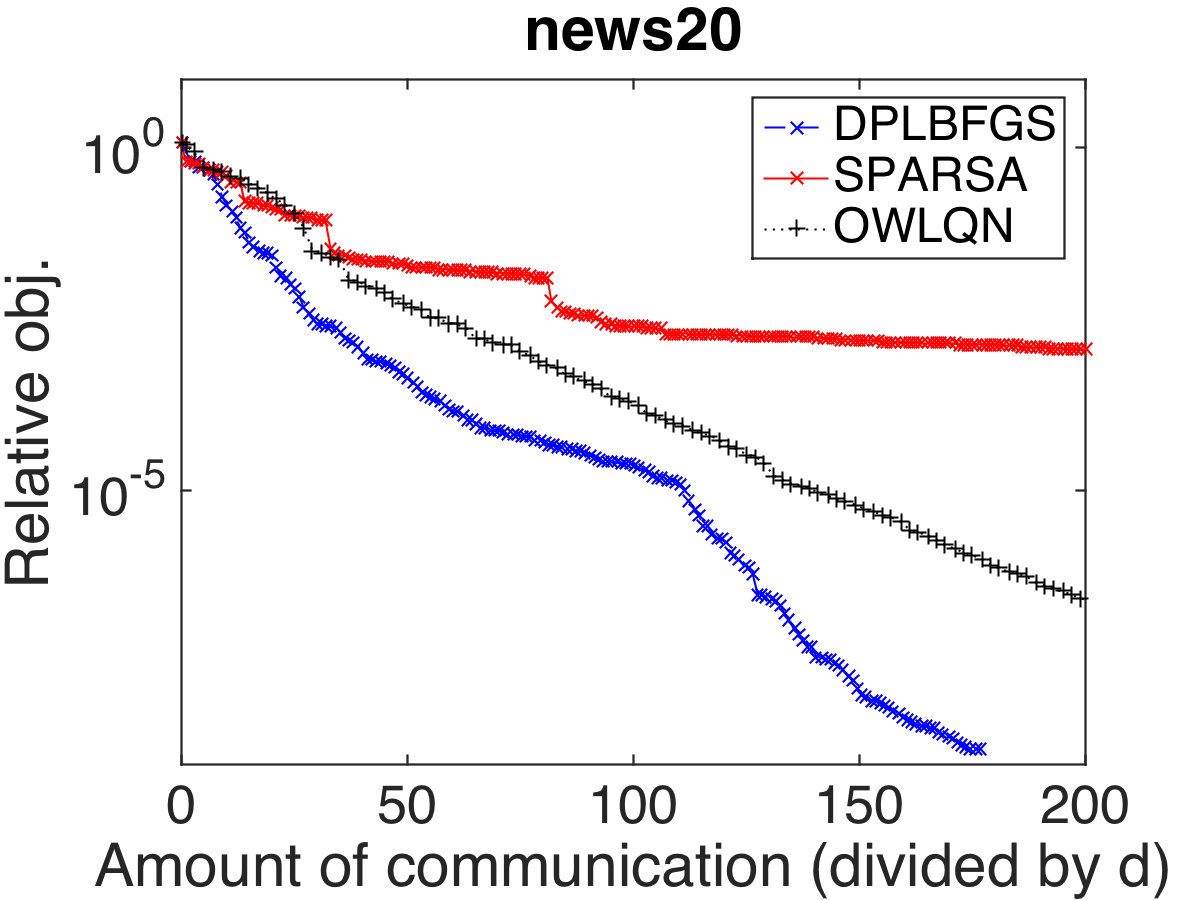
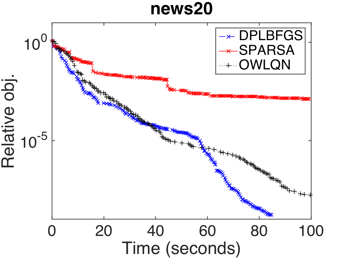
epsilon
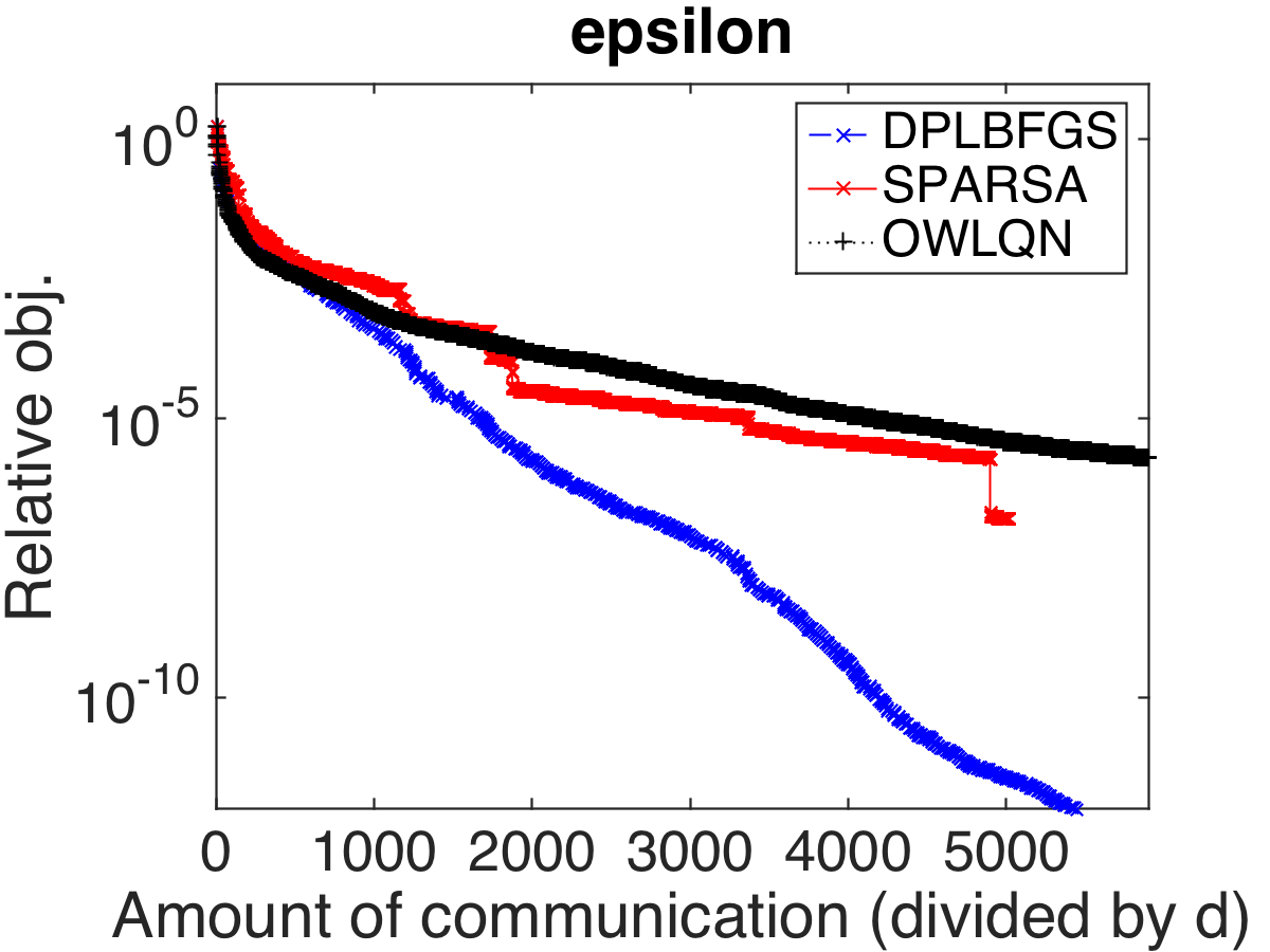
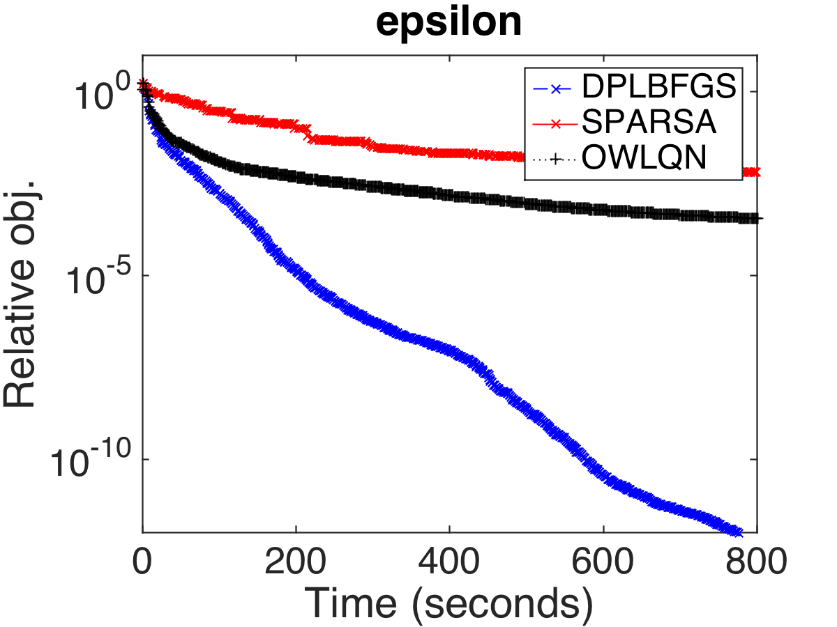
webspam
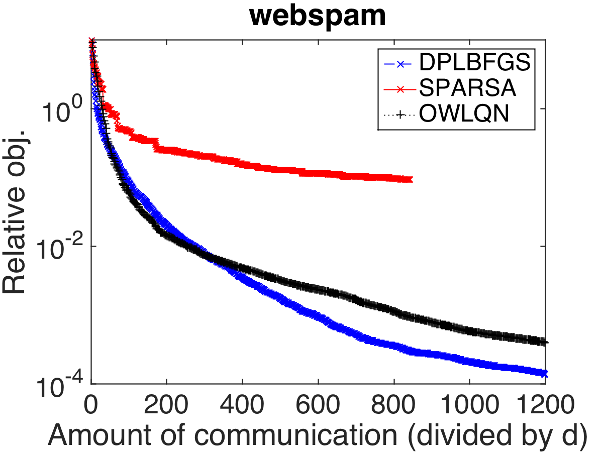
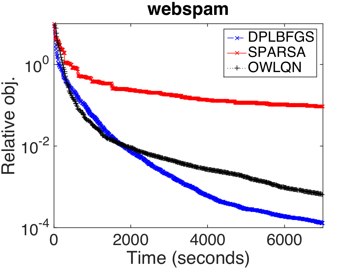
avazu-site

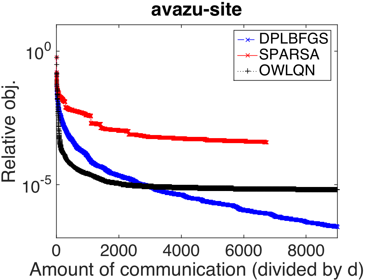
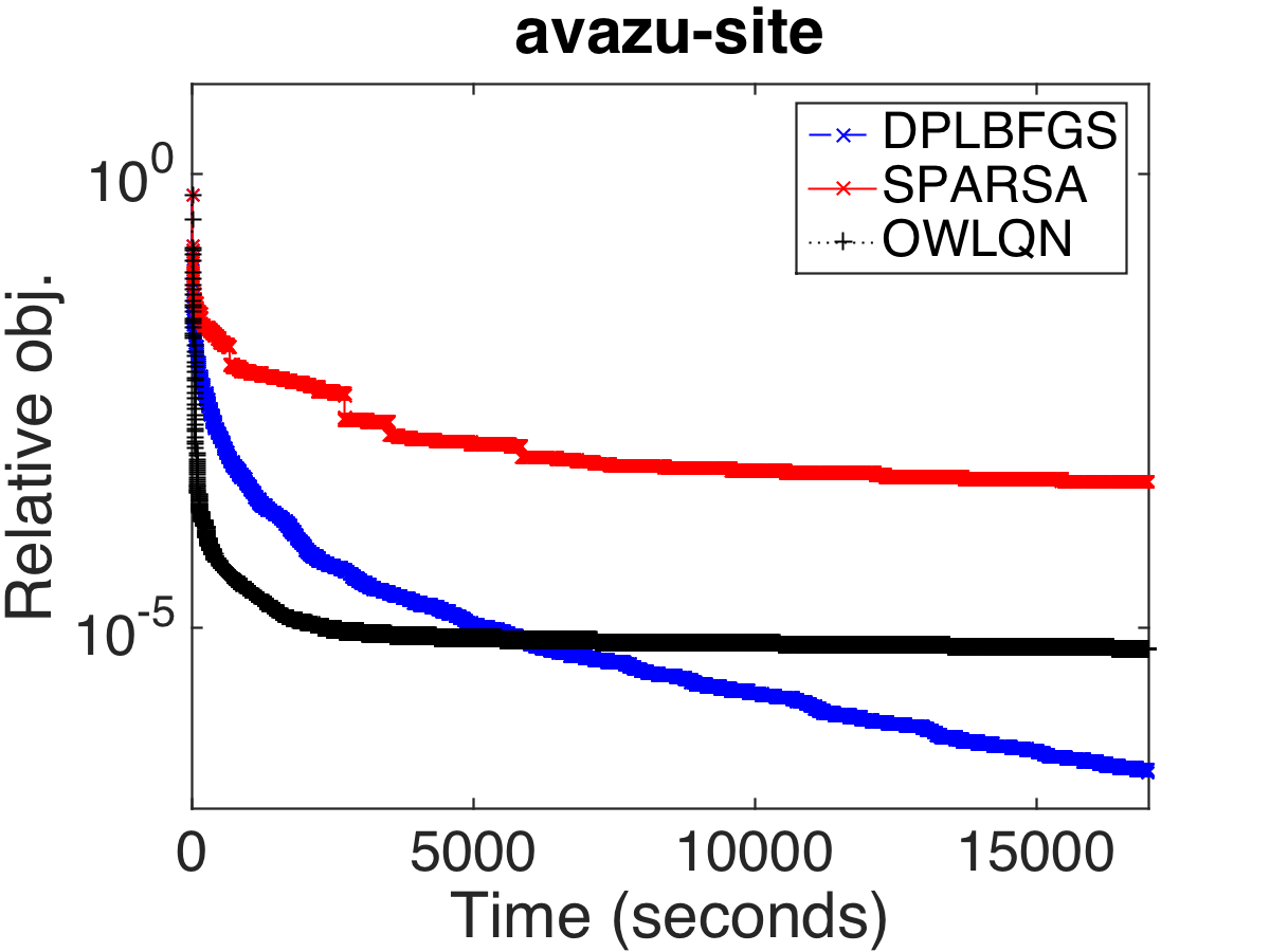
Figure 1. Comparison between different methods for $\ell_{1}$-regularized logistic regression in terms of relative objective difference to the optimum. Left: communication (divided by $d$); right: running time (in seconds).

6. Conclusions

In this work, we propose a practical and communication-efficient distributed algorithm for solving general regularized nonsmooth ERM problems. Our algorithm enjoys fast performance both theoretically and empirically and can be applied to a wide range of ERM problems. It is possible to extend our approach for solving the distributed dual ERM problem with a strongly convex primal regularizer, and we expect our framework to outperform state of the art, which only uses block-diagonal parts of the Hessian that can be computed locally. These topics are left for future work.

Appendix A Proofs

We provide proof of Lemma 3.1 in this section. The rest of Section 3 directly follows the results in Lee and Wright (2018) by noting that $\nabla\tilde{f}({\boldsymbol{w}})$ is $\|X^{T}X\|L$-Lipschitz continuous, and are therefore omitted.

Proof of Lemma 3.1.

We prove the three results separately.

1. The boundedness of $H_{t}$ directly follow from the results in Li and Fukushima (2001). A more detailed proof can be found in, for example, Lee and Wright (2017, Appendix E). The lower bound of $\gamma_{t}$ is directly through (9), and the upper bound is from the Lipschitz continuity of $\nabla\tilde{f}$.

2. By directly expanding $\nabla\hat{f}$, we have that for any ${\boldsymbol{p}}_{1},{\boldsymbol{p}}_{2}$,

   $$\nabla\hat{f}({\boldsymbol{p}}_{1})-\nabla\hat{f}({\boldsymbol{p}}_{2}) =\nabla\tilde{f}({\boldsymbol{w}})+H{\boldsymbol{p}}_{1}-\left(\nabla\tilde{f}({\boldsymbol{w}})+H{\boldsymbol{p}}_{2}\right)$$

   $$=H({\boldsymbol{p}}_{1}-{\boldsymbol{p}}_{2}).$$

   Therefore, we have

   $$\frac{\left(\nabla\hat{f}({\boldsymbol{p}}_{1})-\nabla\hat{f}({\boldsymbol{p}}_{2})\right)^{T}\left({\boldsymbol{p}}_{1}-{\boldsymbol{p}}_{2}\right)}{\left\|{\boldsymbol{p}}_{1}-{\boldsymbol{p}}_{2}\right\|^{2}}=\frac{\left\|{\boldsymbol{p}}_{1}-{\boldsymbol{p}}_{2}\right\|_{H}^{2}}{\left\|{\boldsymbol{p}}_{1}-{\boldsymbol{p}}_{2}\right\|^{2}}\in\left[c_{2},c_{1}\right]$$

   for bounding $\psi_{i}$ for $i>0$, and the bound for $\psi_{0}$ is directly from the bounds of $\gamma_{t}$. The combined bound is therefore $[\min\{c_{2},\delta\},\max\{c_{1},\|X^{T}X\|L\}]$. Next, we show that the final $\psi_{i}$ is always upper-bounded. The right-hand side of (11) is equivalent to the following:

   (25) $$\arg\min_{\boldsymbol{d}}\hat{Q}_{\psi_{i}}\left({\boldsymbol{d}}\right)\coloneqq\nabla\hat{f}({\boldsymbol{p}}^{(i)})^{T}{\boldsymbol{d}}+\frac{\psi_{i}\left\|{\boldsymbol{d}}\right\|^{2}}{2}+\hat{g}\left({\boldsymbol{d}}+{\boldsymbol{p}}\right)-\hat{g}\left({\boldsymbol{p}}\right).$$

   Denote the optimal solution by ${\boldsymbol{d}}^{*}$, then we have ${\boldsymbol{p}}^{(i+1)}={\boldsymbol{p}}^{(i)}+{\boldsymbol{d}}^{*}$. Because $H$ is upper-bounded by $c_{1}$, we have that $\nabla\hat{f}$ is $c_{1}$-Lipschitz continuous. Therefore, using Lemma 12 of Lee and Wright (2018), we get

   (26) $$\hat{Q}_{\psi_{i}}\left({\boldsymbol{d}}^{*}\right)\leq-\frac{\psi_{i}}{2}\left\|{\boldsymbol{d}}^{*}\right\|^{2}.$$

   We then have from $c_{1}$-Lipschitz continuity of $\nabla\hat{f}$ that

   $$~{}Q\left({\boldsymbol{p}}^{(i+1)}\right)-Q\left({\boldsymbol{p}}^{(i)}\right)$$

   $$\leq ~{}\nabla\hat{f}({\boldsymbol{p}}^{(i)})^{T}\left({\boldsymbol{p}}^{(i+1)}-{\boldsymbol{p}}^{(i)}\right)+\frac{c_{1}}{2}\left\|{\boldsymbol{p}}^{(i+1)}-{\boldsymbol{p}}^{(i)}\right\|^{2}$$

   $$\qquad+\hat{g}\left({\boldsymbol{p}}^{(i+1)}\right)-\hat{g}\left({\boldsymbol{p}}^{(i)}\right)$$

   $$\stackrel{{\scriptstyle\eqref{eq:hatQ}}}{{=}} ~{}\hat{Q}_{\psi_{i}}({\boldsymbol{d}}^{*})-\frac{\psi_{i}}{2}\left\|{\boldsymbol{d}}^{*}\right\|^{2}+\frac{c_{1}}{2}\left\|{\boldsymbol{d}}^{*}\right\|^{2}$$

   $$\stackrel{{\scriptstyle\eqref{eq:Qbound}}}{{\leq}} ~{}\left(\frac{c_{1}}{2}-\psi_{i}\right)\|{\boldsymbol{d}}^{*}\|^{2}.$$

   Therefore, whenever

   $$\frac{c_{1}}{2}-\psi_{i}\leq-\frac{\sigma_{0}\psi_{i}}{2},$$

   (13) holds. This is equivalent to

   $$\psi_{i}\geq\frac{c_{1}}{2-\sigma_{0}}.$$

   Since $\sigma_{0}\in(0,1)$, we must have $c_{1}/(2-\sigma_{0})\in(c_{1}/2,c_{1})$, Note that the initialization of $\psi_{i}$ is upper-bounded by $c_{1}$ for all $i>1$, so the final $\psi_{i}$ is upper bounded by $2c_{1}$. Together with the first iteration that we start with $\psi_{0}=\gamma_{t}$, we have that $\psi_{i}$ are always upper-bounded by $\max\{2c_{1},\gamma_{t}\}$, and we have already proven $\gamma_{t}$ is upper-bounded by $\|X^{T}X\|L$.

3. We note that since $Q$ is $c_{2}$-strongly convex, the following condition holds.

   (27) $$\frac{\min_{{\boldsymbol{s}}\in\nabla\hat{f}\left({\boldsymbol{p}}^{(i+1)}\right)+\partial\hat{g}\left({\boldsymbol{p}}^{(i+1)}\right)}\left\|{\boldsymbol{s}}\right\|^{2}}{2c_{2}}\geq Q\left({\boldsymbol{p}}^{(i+1)}\right)-Q^{*}$$

   On the other hand, from the optimality condition of (25), we have that

   (28) $$\psi_{i}{\boldsymbol{d}}^{*}=\nabla\hat{f}\left({\boldsymbol{p}}^{(i)}\right)+{\boldsymbol{s}}_{i+1},$$

   for some

   $${\boldsymbol{s}}_{i+1}\in\partial\hat{g}\left({\boldsymbol{p}}^{(i+1)}\right).$$

   Therefore,

   $$~{}Q\left({\boldsymbol{p}}^{(i+1)}\right)-Q^{*}$$

   $$\stackrel{{\scriptstyle\eqref{eq:kl}}}{{\leq}} ~{}\frac{1}{2c_{2}}\left\|\nabla\hat{f}\left({\boldsymbol{p}}^{(i+1)}\right)-\nabla\hat{f}\left({\boldsymbol{p}}^{(i)}\right)+\nabla\hat{f}\left({\boldsymbol{p}}^{(i)}\right)+{\boldsymbol{s}}_{i+1}\right\|^{2}$$

   $$\stackrel{{\scriptstyle\eqref{eq:dopt}}}{{\leq}} ~{}\frac{1}{c_{2}}\left\|\nabla\hat{f}\left({\boldsymbol{p}}^{(i+1)}\right)-\nabla\hat{f}\left({\boldsymbol{p}}^{(i)}\right)\right\|^{2}+\left\|\psi_{i}{\boldsymbol{d}}^{*}\right\|^{2}$$

   (29) $$\leq ~{}\frac{1}{c_{2}}\left(c_{1}^{2}+\psi^{2}\right)\left\|{\boldsymbol{d}}^{*}\right\|^{2}.$$

   By combining (13) and (29), we obtain

   $$Q\left({\boldsymbol{p}}^{(i+1)}\right)-Q\left({\boldsymbol{p}}^{(i)}\right) \leq-\frac{\sigma_{0}\psi_{i}}{2}\left\|{\boldsymbol{d}}^{*}\right\|^{2}$$

   $$\leq-\frac{\sigma_{0}\psi_{i}}{2}\frac{c_{2}}{c_{1}^{2}+\psi^{2}}\left(Q\left({\boldsymbol{p}}^{(i+1)}\right)-Q^{*}\right).$$

   Rearranging the terms, we obtain

   $$\left(1+\frac{c_{2}\sigma_{0}\psi_{i}}{2(c_{1}^{2}+\psi^{2})}\right)\left(Q\left({\boldsymbol{p}}^{(i+1)}\right)-Q^{*}\right)\leq Q\left({\boldsymbol{p}}^{(i)}\right)-Q^{*},$$

   showing Q-linear convergence of SpaRSA, with

   $$\eta=\left(1+\frac{c_{2}\sigma_{0}\psi_{i}}{2\left(c_{1}^{2}+\psi_{i}^{2}\right)}\right)^{-1}\in[0,1].\qed$$

References

- (1)
- Anderson et al. (1999) Edward Anderson, Zhaojun Bai, Christian Bischof, L Susan Blackford, James Demmel, Jack Dongarra, Jeremy Du Croz, Anne Greenbaum, Sven Hammarling, Alan McKenney, et al. 1999. LAPACK Users’ guide. SIAM.
- Andrew and Gao (2007) Galen Andrew and Jianfeng Gao. 2007. Scalable Training of L1-Regularized Log-Linear Models. In International Conference on Machine Learning.
- Bonettini et al. (2016) Silvia Bonettini, Ignace Loris, Federica Porta, and Marco Prato. 2016. Variable metric inexact line-search-based methods for nonsmooth optimization. SIAM journal on optimization 26, 2 (2016), 891–921.
- Byrd et al. (1994) Richard H. Byrd, Jorge Nocedal, and Robert B. Schnabel. 1994. Representations of quasi-Newton matrices and their use in limited memory methods. Mathematical Programming 63, 1-3 (1994), 129–156.
- Chan et al. (2007) Ernie Chan, Marcel Heimlich, Avi Purkayastha, and Robert Van De Geijn. 2007. Collective communication: theory, practice, and experience. Concurrency and Computation: Practice and Experience 19, 13 (2007), 1749–1783.
- Ghanbari and Scheinberg (2016) Hiva Ghanbari and Katya Scheinberg. 2016. Proximal Quasi-Newton Methods for Convex Optimization. Technical Report. arXiv:1607.03081.
- Lee et al. (2017) Ching-pei Lee, Po-Wei Wang, Weizhu Chen, and Chih-Jen Lin. 2017. Limited-memory Common-directions Method for Distributed Optimization and its Application on Empirical Risk Minimization. In Proceedings of SIAM International Conference on Data Mining.
- Lee and Wright (2017) Ching-pei Lee and Stephen J. Wright. 2017. Using Neural Networks to Detect Line Outages from PMU Data. Technical Report. arXiv:1710.05916.
- Lee and Wright (2018) Ching-pei Lee and Stephen J. Wright. 2018. Inexact Successive Quadratic Approximation for Regularized Optimization. Technical Report.
- Lee et al. (2014) Jason D. Lee, Yuekai Sun, and Michael A. Saunders. 2014. Proximal Newton-type methods for minimizing composite functions. SIAM Journal on Optimization 24, 3 (2014), 1420–1443.
- Li and Fukushima (2001) Dong-Hui Li and Masao Fukushima. 2001. On the global convergence of the BFGS method for nonconvex unconstrained optimization problems. SIAM Journal on Optimization 11, 4 (2001), 1054–1064.
- Lin et al. (2014) Chieh-Yen Lin, Cheng-Hao Tsai, Ching-Pei Lee, and Chih-Jen Lin. 2014. Large-scale logistic regression and linear support vector machines using Spark. In Proceedings of the IEEE International Conference on Big Data. 519–528.
- Liu and Nocedal (1989) Dong C. Liu and Jorge Nocedal. 1989. On the limited memory BFGS method for large scale optimization. Mathematical programming 45, 1 (1989), 503–528.
- Meng et al. (2016) Xiangrui Meng, Joseph Bradley, Burak Yavuz, Evan Sparks, Shivaram Venkataraman, Davies Liu, Jeremy Freeman, DB Tsai, Manish Amde, Sean Owen, et al. 2016. MLlib: Machine learning in Apache Spark. Journal of Machine Learning Research 17, 1 (2016), 1235–1241.
- Message Passing Interface Forum (1994) Message Passing Interface Forum. 1994. MPI: a message-passing interface standard. International Journal on Supercomputer Applications 8, 3/4 (1994).
- Nesterov (1983) Yu Nesterov. 1983. A method of solving a convex programming problem with convergence rate . Soviet Mathematics Doklady 27 (1983), 372–376.
- Nesterov (2013) Yu Nesterov. 2013. Gradient methods for minimizing composite functions. Mathematical Programming 140, 1 (2013), 125–161.