Deep Network Regularization via Bayesian Inference of Synaptic Connectivity

Abstract

Deep neural networks (DNNs) often require good regularizers to generalize well. Currently, state-of-the-art DNN regularization techniques consist in randomly dropping units and/or connections on each iteration of the training algorithm. Dropout and DropConnect are characteristic examples of such regularizers, that are widely popular among practitioners. However, a drawback of such approaches consists in the fact that their postulated probability of random unit/connection omission is a constant that must be heuristically selected based on the obtained performance in some validation set. To alleviate this burden, in this paper we regard the DNN regularization problem from a Bayesian inference perspective: We impose a sparsity-inducing prior over the network synaptic weights, where the sparsity is induced by a set of Bernoulli-distributed binary variables with Beta (hyper-)priors over their prior parameters. This way, we eventually allow for marginalizing over the DNN synaptic connectivity for output generation, thus giving rise to an effective, heuristics-free, network regularization scheme. We perform Bayesian inference for the resulting hierarchical model by means of an efficient Black-Box Variational inference scheme. We exhibit the advantages of our method over existing approaches by conducting an extensive experimental evaluation using benchmark datasets.

1 Introduction

In the last few years, the field of machine learning has experienced a new wave of innovation; this is due to the rise of a family of modeling techniques commonly referred to as deep neural networks (DNNs) [10]. DNNs constitute large-scale neural networks, that have successfully shown their great learning capacity in the context of diverse application areas. Since DNNs comprise a huge number of trainable parameters, it is key that appropriate techniques be employed to prevent them from overfitting. Indeed, it is now widely understood that one of the reasons behind the explosive success and popularity of DNNs consists in the availability of simple, effective, and efficient regularization techniques, developed in the last few years [10].

Dropout is a popular regularization technique for (dense-layer) DNNs [13]. In essence, it consists in randomly dropping different units of the network on each iteration of the training algorithm. This way, only the parameters related to a subset of the network units are trained on each iteration; this ameliorates the associated network overfitting tendency, and it does so in a way that ensures that all network parameters are effectively trained. In a different vein, [14] proposed randomly dropping DNN synaptic connections, instead of network units (and all the associated parameters); they dub this approach DropConnect. As showed therein, such a regularization scheme yields better results than Dropout in several benchmark datasets, while offering provable bounds of computational complexity.

Despite these merits, one drawback of these regularization schemes can be traced to their very foundation and rationale: The postulated probability of random unit/connection omission (e.g., dropout rate) is a constant that must be heuristically selected; this is effected by evaluating the network’s predictive performance under different selections of this probability, in some validation set, and retaining the best performing value. This drawback has recently motivated research on the theoretical properties of these techniques. Indeed, recent theoretical work at the intersection of deep learning and Bayesian statistics has shown that Dropout can be viewed as a simplified approximate Bayesian inference algorithm, and enjoys links with Gaussian process models under certain simplistic assumptions (e.g., [1, 5]).

These recent results form the main motivation behind this paper. Specifically, the main question this work aims to address is the following: Can we devise an effective DNN regularization scheme, that marginalizes over all possible configurations of network synaptic connectivity (i.e., active synaptic connections), with the posterior over them being inferred from the data? To address this problem, in this paper, for the first time in the literature, we regard the DNN regularization problem from the following Bayesian inference perspective: We impose a sparsity-inducing prior over the network synaptic weights, where the sparsity is induced by a set of Bernoulli-distributed binary variables. Further, the parameters of the postulated Bernoulli-distributed binary variables are imposed appropriate Beta (hyper-)priors, which give rise to a full hierarchical Bayesian treatment for the proposed model.

Under this hierarchical Bayesian construction, we can derive appropriate posteriors over the postulated binary variables, which essentially function as indicators of whether some (possible) synaptic connection is retained or dropped from the network. Once these posteriors are obtained using some available training data, prediction can be performed by averaging (under a Bayesian inference sense) over multiple (posterior) samples of the network configuration. This inferential setup constitutes the main point of differentiation between our approach and DropConnect. For simplicity, and to facilitate reference, we dub our approach DropConnect++. We derive an efficient inference algorithm for our model by resorting to the Black-Box Variational Inference (BBVI) scheme [12].

The remainder of this paper is organized as follows: In Section 2, we provide a brief overview of the theoretical background of our approach. Specifically, we first briefly review DropConnect, which is the existing work closest related to our approach; subsequently, we review the inferential framework that will be used in the context of the proposed approach, namely BBVI. In Section 3, we introduce our approach, and derive its inference and prediction generation algorithms. Next, we perform an extensive experimental evaluation of our approach, and compare to popular (dense-layer) DNN regularization approaches, including Dropout and DropConnect. To this end, we consider a number of well-established benchmarks in the related literature. Finally, in the concluding section, we summarize our contribution and discuss our results.

2 Theoretical Background

2.1 DropConnect

As discussed in the Introduction, DropConnect is a generalization of Dropout under which each connection, rather than each unit, may be dropped with some heuristically selected probability. Hence, the rationale of DropConnect is similar to that of Dropout, since both introduce dynamic sparsity within the model. Their core difference consists in the fact that Dropout imposes sparsity on the output vectors of a (dense) layer, while DropConnect imposes sparsity on the synaptic weights $\boldsymbol{W}$.

Note that this is not equivalent to setting $\boldsymbol{W}$ to be a fixed sparse matrix during training. Indeed, for a DropConnect layer, the output is given as [14]:

$$\boldsymbol{r}=a((\boldsymbol{Z}\circ\boldsymbol{W})\boldsymbol{v})$$ (1)

where $\circ$ is the elementwise product, $a(\cdot)$ is the adopted activation function, $\boldsymbol{W}$ is the matrix of synaptic weights, $\boldsymbol{v}$ is the layer input vector, and $\boldsymbol{r}$ is the layer output vector. Further, $\boldsymbol{Z}$ is a matrix of binary variables (indicators) encoding the connection information, with

$$[\boldsymbol{Z}]_{i,j}\sim\mathrm{Bernoulli}(p)$$ (2)

where $p$ is a heuristically selected probability. Hence, DropConnect is a generalization of Dropout to the full connection structure of a layer [14].

Training of a DropConnect layer begins by selecting an example $\boldsymbol{v}$, and drawing a mask matrix $\boldsymbol{Z}$ from a $\mathrm{Bernoulli}(p)$ distribution to mask out elements of both the weight matrix and the biases in the DropConnect layer. The parameters throughout the model can be updated via stochastic gradient descent (SGD), or some modern variant of it, by backpropagating gradients of the postulated loss function with respect to the parameters. To update the weight matrix $\boldsymbol{W}$ in a DropConnect layer, the mask is applied to the gradient to update only those elements that were active in the forward pass. Additionally, when passing gradients down, the masked weight matrix $\boldsymbol{Z}\circ\boldsymbol{W}$ is used.

2.2 BBVI

In general, Bayesian inference for a statistical model can be performed either exactly, by means of Markov Chain Monte Carlo (MCMC), or via approximate techniques. Variational inference is the most widely used approximate technique; it approximates the posterior with a simpler distribution, and fits that distribution so as to have minimum Kullback-Leibler (KL) divergence from the exact posterior [8]. This way, variational inference effectively converts the problem of approximating the posterior into an optimization problem.

One of the significant drawbacks of traditional variational inference consists in the fact that its objective entails posterior expectations which are tractable only in the case of conjugate postulated models. Hence, recent innovations in variational inference have attempted to allow for rendering it feasible even in cases of more complex, non-conjugate model formulations. Indeed, recently proposed solutions to this problem consist in using stochastic optimization, by forming noisy gradients with Monte Carlo (MC) approximation. In this context, a number of different techniques have been proposed so as to successfully reduce the unacceptably high variance of conventional MC estimators. BBVI [12] is one of these recently proposed alternatives, amenable to non-conjugate probabilistic models that entail both discrete and continuous latent variables.

Let us consider a probabilistic model $p(\boldsymbol{x},\boldsymbol{z})$ with observations $\boldsymbol{x}$ and latent variables $\boldsymbol{z}$, as well as a sought variational family $q(\boldsymbol{z};\boldsymbol{\phi})$. BBVI optimizes an evidence lower bound (ELBO), with expression

$$\mathrm{log}\,p(\boldsymbol{x})\geq\mathcal{L}(\boldsymbol{\phi})=\mathbb{E}_{q(\boldsymbol{z};\boldsymbol{\phi})}[\mathrm{log}\,p(\boldsymbol{x},\boldsymbol{z})-\mathrm{log}\,q(\boldsymbol{z};\boldsymbol{\phi})]$$ (3)

This is performed by relying on the “log-derivative trick” [7, 15] to obtain MC estimates of the gradient. Specifically, by application of the identities

$$\nabla_{\boldsymbol{\phi}}q(\boldsymbol{z};\boldsymbol{\phi})=q(\boldsymbol{z};\boldsymbol{\phi})\nabla_{\boldsymbol{\phi}}\mathrm{log}\,q(\boldsymbol{z};\boldsymbol{\phi})$$ (4)

$$\mathbb{E}_{q(\boldsymbol{z};\boldsymbol{\phi})}[\nabla_{\boldsymbol{\phi}}\mathrm{log}\,q(\boldsymbol{z};\boldsymbol{\phi})]=0$$ (5)

the gradient of the ELBO (3) reads

$$\nabla_{\boldsymbol{\phi}}\mathcal{L}(\boldsymbol{\phi})=\mathbb{E}_{q(\boldsymbol{z};\boldsymbol{\phi})}[f(\boldsymbol{z})]$$ (6)

where

$$f(\boldsymbol{z})=\nabla_{\boldsymbol{\phi}}\mathrm{log}\,q(\boldsymbol{z};\boldsymbol{\phi})\left[\mathrm{log}\,p(\boldsymbol{x},\boldsymbol{z})-\mathrm{log}\,q(\boldsymbol{z};\boldsymbol{\phi})\right]$$ (7)

The so-obtained MC estimator, based on computing the posterior expectations $\mathbb{E}_{q(\boldsymbol{z};\boldsymbol{\phi})}[\cdot]$ via sampling from $q(\boldsymbol{z};\boldsymbol{\phi})$, only requires evaluating the log-joint distribution $\mathrm{log}\,p(\boldsymbol{x},\boldsymbol{z})$, the log-variational distribution $\mathrm{log}\,q(\boldsymbol{z};\boldsymbol{\phi})$, and the score function $\nabla_{\boldsymbol{\phi}}\mathrm{log}\,q(\boldsymbol{z};\boldsymbol{\phi})$, which is easy for a large class of models. However, the resulting estimator may have high variance, especially if the variational approximation $q(\boldsymbol{z};\boldsymbol{\phi})$ is a poor fit to the actual posterior. In order to reduce the variance of the estimator, one common strategy in BBVI consists in the use of control variates.

A control variate is a random variable that is included in the estimator, preserving its expectation but reducing its variance. The most usual choice for control variates, which we adopt in this work, is the so-called weighted score function: Under this selection, the ELBO gradient becomes

$$\nabla_{\boldsymbol{\phi}}\mathcal{L}(\boldsymbol{\phi})=\mathbb{E}_{q(\boldsymbol{z};\boldsymbol{\phi})}[f(\boldsymbol{z})-\varpi h(\boldsymbol{z})]$$ (8)

where the score function reads

$$h(\boldsymbol{z})=\nabla_{\boldsymbol{\phi}}\mathrm{log}\,q(\boldsymbol{z};\boldsymbol{\phi})$$ (9)

while the weights $\varpi$ yield the (optimized) expression [12]

$$\varpi=\frac{\mathrm{Cov}\left(f(\boldsymbol{z}),h(\boldsymbol{z})\right)}{\mathrm{Var}\left(h(\boldsymbol{z})\right)}$$ (10)

On this basis, derivation of the sought variational posteriors is performed by utilizing the gradient expression (8) in the context of popular, off-the-shelf optimization algorithms, e.g. AdaM [9] and Adagrad [4].

3 Proposed Approach

The output expression of a DropConnect++ layer is fundamentally similar to conventional DropConnect, and is given by (1). However, DropConnect++ introduces an additional hierarchical set of assumptions regarding the matrix of binary (mask) variables $\boldsymbol{Z}=[z_{ij}]_{i,j}$, which indicate whether a synaptic connection is inferred to be on or off.

Specifically, as usual in hierarchical graphical models, we assume that the random matrix $\boldsymbol{Z}$ is drawn from an appropriate prior; we postulate

$$p(\boldsymbol{Z}|\boldsymbol{\Pi})=\prod_{i,j}p(z_{ij}|\pi_{ij})=\prod_{i,j}\mathrm{Bernoulli}(z_{ij}|\pi_{ij})$$ (11)

Subsequently, to facilitate further regularization for DropConnect++ layers under a Bayesian inferential perspective, the prior parameters $\pi_{ij}\triangleq p(z_{ij}=1)$ are imposed their own (hyper-)prior. Specifically, we elect to impose a Beta hyper-prior, yielding

$$p(\pi_{ij}|\alpha,\beta)=\mathrm{Beta}(\pi_{ij}|\alpha,\beta),\;\forall i,j$$ (12)

Under this definition, to train a postulated DNN incorporating DropConnect++ layers, we need to resort to some sort of Bayesian inference technique. In this paper, we resort to BBVI, as we explain next.

3.1 Training DNNs with DropConnect++ layers

Let us consider a DNN the observed training data of which constitute the set $\mathcal{D}=\{\boldsymbol{d}_{n}\}_{n=1}^{N}$. In case of a generative modeling scheme, each example $\boldsymbol{d}_{n}$ is a single observation, say $\boldsymbol{x}_{n}$, from the distribution we wish to model. On the other hand, in case of a discriminative modeling task, each example $\boldsymbol{d}_{n}$ is an input/output pair, for instance $\boldsymbol{d}_{n}=(\boldsymbol{x}_{n},\boldsymbol{y}_{n})$. In both cases, conventional DNN training consists in optimizing a negative loss function, measuring the fit of the model to the training dataset $\mathcal{D}$. Such measures can be equivalently expressed in terms of a log-likelihood function $\mathrm{log}\,p(\mathcal{D})$; under this regard, DNN training effectively boils down to maximum-likelihood estimation [3, 6].

The deviation of a DNN comprising DropConnect++ layers from this simple training scheme stems from obtaining appropriate posterior distributions over the latent variables of DropConnect++, namely the binary indicator matrices of synaptic connectivity, $\boldsymbol{Z}$, as well as the associated parameters with hyper-priors imposed over them, namely the matrices of (prior) parameters $\boldsymbol{\Pi}$. To this end, DropConnect++ postulates separate posteriors over each entry of the random matrices $\boldsymbol{Z}$, that correspond to each individual synapse, $(i,j)$:

$$q(\boldsymbol{Z})=\prod_{i,j}q(z_{ij}|\tilde{\pi}_{ij}),\mathrm{\;with:}\qquad q(z_{ij}|\tilde{\pi}_{ij})=\mathrm{Bernoulli}(z_{ij}|\tilde{\pi}_{ij})$$ (13)

Further, we consider that the matrices of prior parameters, $\boldsymbol{\Pi}$, yield a factorized (hyper-)posterior with Beta-distributed factors of the form

$$q(\pi_{ij})=\mathrm{Beta}(\pi_{ij}|\tilde{\alpha}_{ij},\tilde{\beta}_{ij})$$ (14)

Our construction entails a conditional log-likelihood term, $\mathrm{log}\,p(\mathcal{D}|\boldsymbol{Z})$. This is similar to a conventional DNN, with the weight matrices $\boldsymbol{W}$ at each layer multiplied with the corresponding latent indicator (mask) matrices, $\boldsymbol{Z}$ (in analogy to DropConnect). The corresponding posterior expectation term, $\mathbb{E}_{q(\boldsymbol{Z})}[\mathrm{log}\,p(\mathcal{D}|\boldsymbol{Z})]$, constitutes part of the ELBO expression of our model. Unfortunately, this term is analytically intractable due to the entailed nonlinear dependencies on the indicator matrix $\boldsymbol{Z}$, which stem from the nonlinear activation function $a(\cdot)$. Following the previous discussion, we ameliorate this issue by resorting to an efficient approximation obtained by drawing MC samples. The so-obtained ELBO functional expression eventually becomes:

$$\mathcal{L}(\mathcal{D})\approx -\sum_{i,j}\mathrm{KL}\big{[}q(z_{ij}|\tilde{\pi}_{ij})||p(z_{ij}|\pi_{ij})\big{]}-\sum_{i,j}\mathrm{KL}\big{[}q(\pi_{ij}|\tilde{\alpha}_{ij},\tilde{\beta}_{ij})||p(\pi_{ij}|\alpha,\beta)\big{]}$$ (15)

$$+\frac{1}{L}\sum_{l,n=1}^{L,N}\mathrm{log}\,p(\boldsymbol{d}_{n}|\boldsymbol{Z}^{(l)})$$

where $L$ is the number of samples, $\boldsymbol{Z}^{(l)}=[z_{ij}^{(l)}]_{i,j}$ and $z_{ij}^{(l)}\sim\mathrm{Bernoulli}(z_{ij}|\tilde{\pi}_{ij})$.

This concludes the formulation of the proposed inferential setup for a DNN that contains DropConnect++ layers. On this basis, inference is performed by resorting to BBVI, which proceeds as described previously. Denoting $\tilde{\boldsymbol{\pi}}=(\tilde{\pi}_{ij})_{i,j},\tilde{\boldsymbol{\alpha}}=(\tilde{\alpha}_{ij})_{i,j},\tilde{\boldsymbol{\beta}}=(\tilde{\beta}_{ij})_{i,j}$, the used ELBO gradient reads

$$\nabla_{\tilde{\boldsymbol{\pi}},\tilde{\boldsymbol{\alpha}},\tilde{\boldsymbol{\beta}},\boldsymbol{W}}\mathcal{L}(\mathcal{D})\approx \frac{1}{L}\sum_{l,n=1}^{L,N}\nabla_{\boldsymbol{W}}\mathrm{log}\,p(\boldsymbol{d}_{n}|\boldsymbol{Z}^{(l)})-\sum_{i,j}\nabla_{\tilde{\boldsymbol{\pi}},\tilde{\boldsymbol{\alpha}},\tilde{\boldsymbol{\beta}}}\mathrm{KL}\big{[}q(z_{ij}|\tilde{\pi}_{ij})||p(z_{ij}|\pi_{ij})\big{]}$$ (16)

$$-\sum_{i,j}\nabla_{\tilde{\boldsymbol{\alpha}},\tilde{\boldsymbol{\beta}}}\mathrm{KL}\big{[}q(\pi_{ij}|\tilde{\alpha}_{ij},\tilde{\beta}_{ij})||p(\pi_{ij}|\alpha,\beta)\big{]}$$

$$-\varpi\sum_{i,j}\nabla_{\tilde{\boldsymbol{\pi}},\tilde{\boldsymbol{\alpha}},\tilde{\boldsymbol{\beta}}}[\mathrm{log}\,q(z_{ij}|\tilde{\pi}_{ij})+q(\pi_{ij}|\tilde{\alpha}_{ij},\tilde{\beta}_{ij})]$$

where $\varpi$ is defined in (10). As one can note, we do not perform Bayesian inference for the synaptic weight parameters $\boldsymbol{W}$. Instead, we obtain point-estimates, similar to conventional DropConnect.

3.2 Feedforward computation in DNNs with DropConnect++ layers

Computation of the output of a trained DNN with DropConnect++ layers, given some network input $\boldsymbol{x}_{*}$, requires that we come up with an appropriate solution to the problem of computing the posterior expectation of the DropConnect++ layers output, say $\boldsymbol{r}_{*}$.

Let us consider a DropConnect++ layer with input $\boldsymbol{v}_{*}$ (corresponding to a DNN input observation $\boldsymbol{x}_{*}$); we have

$$\boldsymbol{r}_{*}=\mathbb{E}_{q(\boldsymbol{Z})}[a((\boldsymbol{Z}\circ\boldsymbol{W})\boldsymbol{v}_{*})]$$ (17)

This computation essentially consists in marginalizing out the layer synaptic connectivity structure, by appropriately utilizing the variational posterior distribution $q(\boldsymbol{Z})$, learned by means of BBVI, as discussed in the previous Section. Unfortunately, this posterior expectation cannot be computed analytically, due to the nonlinear activation function $a(\cdot)$.

This problem can be solved by approximating (17) via simple MC sampling:

$$\boldsymbol{r}_{*}\approx\frac{1}{L}\sum_{l=1}^{L}a((\boldsymbol{Z}^{(l)}\circ\boldsymbol{W})\boldsymbol{v}_{*})$$ (18)

where the $\boldsymbol{Z}^{(l)}$ are drawn from $q(\boldsymbol{Z})$. However, an issue such an approach suffers from is the need to retain in memory large sample matrices $\{\boldsymbol{Z}^{(l)}\}_{l=1}^{L}$, that may comprise millions of entries, in cases of large-scale DNNs. To completely alleviate such computational efficiency issues, in this work we opt for an alternative approximation that reads

$$\boldsymbol{r}_{*}\approx a((\tilde{\boldsymbol{\Pi}}\circ\boldsymbol{W})\boldsymbol{v}_{*})$$ (19)

where the matrix $\tilde{\boldsymbol{\Pi}}=[\tilde{\pi}_{ij}]_{i,j}$ is obtained from the model training algorithm, described previously. Note that such an approximation is similar to the solution adopted by Dropout [13], which undoubtedly constitutes the most popular DNN regularization technique to date. We shall examine how this solution compares to MC sampling in the experimental section of this work.

Table 1: Predictive accuracy (%) of the evaluated methods.

Method	CIFAR-10	CIFAR-100	SVHN	NORB
No regularization	74.47	41.96	90.53	90.55
Dropout	75.70	46.65	92.14	92.07
DropConnect	76.06	46.12	91.41	91.88
DropConnect++	76.54	47.01	91.99	93.75

Table 2: Computational complexity per iteration at training time ($L=1$).

#Method	CIFAR-10	CIFAR-100	SVHN	NORB
No regularization	9s	10s	15s	5s
Dropout	9s	10s	15s	5s
DropConnect	9s	10s	15s	5s
DropConnect++	10s	13s	19s	6s

4 Experimental Evaluation

To empirically evaluate the performance of our approach, we consider a number of supervised learning experiments, using the CIFAR-10, CIFAR-100, SVHN, and NORB benchmarks. In all our experiments, the used datasets are normalized with local zero mean and unit variance; no other pre-processing is implemented in this work. To obtain some comparative results, apart from our method we also evaluate in our experiments DNNs with similar architecture but: (i) application of no regularization technique; (ii) regularized via Dropout; and (iii) regularized via DropConnect.

In all cases, we use Adagrad with minibatch size equal to 128. Adagrad’s global stepsize is chosen from the set $\{0.005,0.01,0.05\}$, based on the network performance on the training set in the first few iterations. The units of all the postulated DNNs comprise ReLU nonlinearities [11]. Initialization of the network parameters is performed via Glorot-style uniform initialization [6]. To account for the effects of random initialization on the observed performances, we repeat our experiments 50 times; we report the resulting mean accuracies, and run the Student’s-t statistical significance test to examine the statistical significance of the reported performance differences.

Prediction generation using our method is performed by employing the efficient approximation (19). The alternative approach of relying on MC sampling to perform feedforward computation [Eq. (18)] is evaluated in Section 4.2. In all cases, we set the prior hyperparameters of DropConnect++ to $\alpha=\beta=1$; this is a convenient selection which reflects that we have no preferred values for the priors $\pi_{ij}$. The Dropout and DropConnect rates are selected on the grounds of performance maximization, following the selection procedures reported in the related literature. Our source codes have been developed in Python, using the Theano [2] and Lasagne libraries. We run our experiments on an Intel Xeon 2.5GHz Quad-Core server with 64GB RAM and an NVIDIA Tesla K40 GPU.

CIFAR-10

The CIFAR-10 dataset consists of color images of size 32$\times$32, that belong to 10 categories (airplanes, automobiles, birds, cats, deers, dogs, frogs, horses, ships, trucks). We perform our experiments using the available 50,000 training samples and 10,000 test samples. All the evaluated methods comprise a convolutional architecture with three layers, 32 feature maps in the first layer, 32 feature maps in the second layer, 64 feature maps in the third layer, a $5\times 5$ filter size, and a max-pooling sublayer with a pool size of 3$\times$3. These three layers are followed by a dense layer with 64 hidden units, regularized via Dropout, DropConnect, or DropConnect++. The resulting performance statistics (predictive accuracy) of the evaluated methods are depicted in the first column of Table 1. As we observe, our approach outperforms all the considered competitors.

CIFAR-100

The CIFAR-100 dataset consists of 50,000 training and 10,000 testing color images of size 32$\times$32, that belong to 100 categories. We retain this split of the data into a training set and a test set in the context of our experiments. The trained DNN comprises three convolutional layers of same architecture as the ones adopted in the CIFAR-10 experiment, that are followed by a dense layer comprising 512 hidden units. As we show in Table 1, our approach outperforms all its competitors, yielding the best predictive performance. Note also that the DropConnect method, which is closely related to our approach, yields in this experiment worse results than Dropout.

SVHN

The Street View House Numbers (SVHN) dataset consists of 73,257 training and 26,032 test color images of size 32x32; these depict house numbers collected by Google Street View. We retain this split of the data into a training set and a test set in the context of our experiments, and adopt exactly the same DNN architecture as in the CIFAR-100 experiment. As we show in Table 1, our method improves over the related DropConnect method.

NORB

The NORB (small) dataset comprises a collection of stereo images of 3D models that belong to 6 classes (animal, human, plane, truck, car, blank). We downsample the images from 96$\times$96 to 32$\times$32, and perform training and testing using the provided dataset split. We train DNNs with architecture similar to the one adopted in the context of the SVHN and CIFAR-100 datasets. As we show in Table 1, our method outperforms all the considered competitors.

Table 3: Variation of the predictive accuracy (%) of the MC-driven approach (18) with the number of MC samples.

#Samples, $L$	CIFAR-10	CIFAR-100	SVHN	NORB
1	74.57	43.28	91.32	90.04
30	75.95	46.33	91.70	90.78
50	76.01	46.33	91.72	91.04
100	76.01	46.54	91.78	91.41
500	76.36	46.94	91.78	91.58

4.1 Computational complexity

Another significant aspect that affects the efficacy of a regularization technique is its final computational costs, and how they compare to the competition. To allow for investigating this aspect, in Table 2 we illustrate the time needed to complete one iteration of the training algorithms of the evaluated networks in our implementation. As we observe, the training algorithm of our approach imposes an 11%-30% increase in the computational time per iteration, depending on the sizes of the network and the dataset. Note though that DNN training is an offline procedure; hence, a relatively small increase in the required training time is reasonable, given the observed predictive performance gains.

On the other hand, when it comes to using a trained DNN for prediction generation (test time), we emphasize that the computational costs of our approach are exactly the same as in the case of Dropout. This is, indeed, the case due to our utilization of the approximation (19), which results in similar feedforward computations for DropConnect++ as in the case of Dropout.

4.2 Further investigation

A first issue that requires deeper investigation concerns the statistical significance of the observed performance differences. Application of the Student’s-t test on the obtained sets of performances of each method (after 50 experiment repetitions from different random starts) has shown that these differences are statistically significant among all relevant pairs of methods (i.e. DropConnect++ vs. DropConnect, DropConnect++ vs. DropOut, and DropConnect++ vs. no regularization); only exception is the SVHN dataset, where DropConnect++ and DropOut are shown to be of statistically comparable performance.

Further, in Table 3 we show how the predictive performance of DropConnect++ changes if we perform feedforward computation via MC sampling, as described in Eq. (18). As we observe, using only one MC sample results in rather poor performance; this changes fast as we increase the number of samples. However, it appears that even with a high number of drawn samples, the MC-driven approach (18) does not yield any performance improvement over the approximation (19), despite imposing considerable computational overheads.

Further, in Fig. 1(a) we illustrate predictive accuracy convergence; for demonstration purposes, we consider the experimental case of the CIFAR-10 benchmark. Our exhibition concerns both application of the approximate feedforward computation rule (19), as well as resorting to MC sampling. We observe a clear and consistent convergence pattern in both cases.

Finally, it is interesting to get a feeling of the values that take the inferred posterior probabilities, $\tilde{\boldsymbol{\pi}}$, of synaptic connectivity. In Fig. 1(b), we illustrate the inferred values of $\tilde{\boldsymbol{\pi}}$ for all the network synapses, in the case of the CIFAR-10 experiment. As we observe, out of the almost 300K synapses, around 50K take values less than 0.35, another 50K take values greater than 0.6, while the rest 200K take values approximately in the interval $[0.4,0.6]$. This implies that, out of the total 300K postulated synapses, almost half of them are most likely to be omitted during inference. Most significantly, this figure depicts that our approach infers (in a data-driven fashion) which specific synapses are most useful to the network (thus yielding relatively high values of $\tilde{\pi}_{ij}$), and which should rather be omitted. This is in contrast to existing approaches, which merely apply a homogeneous, random omission/retention rate on each layer.

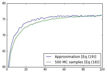
(a)

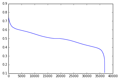
(b)

Figure 1: (a) Accuracy convergence. (b) Inferred posterior probabilities, $\tilde{\boldsymbol{\pi}}$.

5 Conclusions

In this paper, we examined whether there is a feasible way of performing DNN regularization by marginalizing over network synaptic connectivity in a Bayesian manner. Specifically, we sought to derive an appropriate posterior distribution over the network synaptic connectivity, inferred from the data. To this end, we imposed a sparsity-inducing prior over the network synaptic weights, where the sparsity is induced by a set of Bernoulli-distributed binary variables. Further, we imposed appropriate Beta (hyper-)priors over the parameters of the postulated Bernoulli-distributed binary variables. Under this hierarchical Bayesian construction, we obtained appropriate posteriors over the postulated binary variables, which indicate which synaptic connections are retained and which or dropped during inference. This was effected in an efficient and elegant fashion, by resorting to BBVI. We performed an extensive experimental evaluation, using several benchmark datasets. In most cases, our approach yielded a statistically significant performance improvement, for competitive computational costs.

Acknowledgment

We gratefully acknowledge the support of NVIDIA Corporation with the donation of one Tesla K40 GPU used for this research.

Appendix

$$\mathrm{KL}[q(z_{ij}|\tilde{\pi}_{ij})||p(z_{ij}|\pi_{ij})\big{]} =\tilde{\pi}_{ij}\mathrm{log}\tilde{\pi}_{ij}+(1-\tilde{\pi}_{ij})\mathrm{log}(1-\tilde{\pi}_{ij})$$ (20)

$$-\tilde{\pi}_{ij}\mathbb{E}_{q(\pi_{ij})}[\mathrm{log}\pi_{ij}]-(1-\tilde{\pi}_{ij})\mathbb{E}_{q(\pi_{ij})}[\mathrm{log}(1-\pi_{ij})]$$

$$\mathrm{KL}\big{[}q(\pi_{ij}|\tilde{\alpha}_{ij},\tilde{\beta}_{ij})||p(\pi_{ij}|\alpha,\beta)\big{]} =\mathrm{log}\Gamma(\tilde{\alpha}_{ij}+\tilde{\beta}_{ij})-\mathrm{log}\Gamma(\tilde{\alpha}_{ij})-\mathrm{log}\Gamma(\tilde{\beta}_{ij})$$ (21)

$$+(\tilde{\alpha}_{ij}-\alpha) \mathbb{E}_{q(\pi_{ij})}[\mathrm{log}\pi_{ij}]+(\tilde{\beta}_{ij}-\beta)\mathbb{E}_{q(\pi_{ij})}[\mathrm{log}(1-\pi_{ij})]$$

where:

$$\mathbb{E}_{q(\pi_{ij})}[\mathrm{log}\pi_{ij}]=\psi(\tilde{\alpha}_{ij})-\psi(\tilde{\alpha}_{ij}+\tilde{\beta}_{ij})$$ (22)

$$\mathbb{E}_{q(\pi_{ij})}[\mathrm{log}(1-\pi_{ij})]=\psi(\tilde{\beta}_{ij})-\psi(\tilde{\alpha}_{ij}+\tilde{\beta}_{ij})$$ (23)

$\Gamma(\cdot)$ is the Gamma function, and $\psi(\cdot)$ is the Digamma function.

References

- [1] Baldi, P., Sadowski, P.: Understanding dropout. In: Proc. NIPS (2013)
- [2] Bastien, F., Lamblin, P., Pascanu, R., Bergstra, J., Goodfellow, I.J., Bergeron, A., Bouchard, N., Bengio, Y.: Theano: new features and speed improvements. Deep Learning and Unsupervised Feature Learning NIPS 2012 Workshop (2012)
- [3] Bengio, Y., Yao, L., Alain, G., Vincent, P.: Generalized denoising autoencoders as generative models. In: Proc. NIPS. pp. 899– 907 (2013)
- [4] Duchi, J., Hazan, E., Singer, Y.: Adaptive subgradient methods for online learning and stochastic optimization. J. Machine Learning Research 12, 2121– 2159 (2010)
- [5] Gal, Y., Ghahramani, Z.: Dropout as a Bayesian approximation: Insights and applications. In: Deep Learning Workshop, ICML (2015)
- [6] Glorot, X., Bengio, Y.: Understanding the difficulty of training deep feedforward neural networks. In: Proc. AISTATS (2010)
- [7] Glynn, P.W.: Likelihood ratio gradient estimation for stochastic systems. Communications of the ACM 33(10), 75–84 (1990)
- [8] Jaakkola, T., Jordan, M.: Bayesian parameter estimation via variational methods. Statistics and Computing 10, 25–37 (2000)
- [9] Kingma, D., Ba, J.: Adam: A method for stochastic optimization. In: Proc. ICLR (2015)
- [10] LeCun, Y., Bengio, Y., Hinton, G.: Deep learning. Nature 512, 436–444 (2015)
- [11] Nair, V., Hinton, G.: Rectified linear units improve restricted Boltzmann machines. In: Proc. ICML (2010)
- [12] Ranganath, R., Gerrish, S., Blei, D.M.: Black box variational inference. In: Proc. AISTATS (2014)
- [13] Srivastava, N., Hinton, G.E., Krizhevsky, A., Sutskever, I., Salakhutdinov, R.R.: Dropout: A simple way to prevent neural networks from overfitting. J. Machine Learning Research 15(6), 1929–1958 (June 2014)
- [14] Wan, L., Zeiler, M., Zhang, S., LeCun, Y., Fergus, R.: Regularization of neural networks using DropConnect. In: Proc. ICML (2013)
- [15] Williams, R.J.: Simple statistical gradient-following algorithms for connectionist reinforcement learning. Machine Learning 8(3-4), 229–256 (1992)