Training Deep Learning Based Denoisers without Ground Truth Data

Abstract

Recently developed deep-learning-based denoisers often outperform state-of-the-art conventional denoisers such as the BM3D. They are typically trained to minimize the mean squared error (MSE) between the output image of a deep neural network (DNN) and a ground truth image. Thus, it is important for deep-learning-based denoisers to use high quality noiseless ground truth data for high performance. However, it is often challenging or even infeasible to obtain noiseless images in some applications. Here, we propose a method based on Stein’s unbiased risk estimator (SURE) for training DNN denoisers based only on the use of noisy images in the training data with Gaussian noise. We demonstrate that our SURE-based method, without the use of ground truth data, is able to train DNN denoisers to yield performances close to those networks trained with ground truth for both grayscale and color images. We also propose a SURE-based refining method with a noisy test image for further performance improvement. Our quick refining method outperformed conventional BM3D, deep image prior, and often the networks trained with ground truth. Potential extension of our SURE-based methods to Poisson noise model was also investigated.

1 Introduction

Deep neural network (DNN) has been successfully used in various high-level computer vision tasks, such as image classification [1, 2, 3], object detection [4, 5, 6], semantic segmentation [7, 8, 9], and image generation [10, 11, 12]. DNN has also been investigated for low-level computer vision tasks, such as image denoising [13, 14, 15, 16, 17], image inpainting [18, 19, 20], image super resolution [21, 22, 23], and image restoration [24, 25, 26]. In particular, image denoising is a fundamental computer vision task that yields images with reduced noise, and improves the execution of other tasks, such as image classification [13] and image restoration [26].

Deep learning based image denoisers have yielded performances that are equivalent to or better than those of conventional state-of-the-art denoising techniques such as BM3D [27]. These deep denoisers typically train their networks by minimizing the mean-squared error (MSE) between the output of a network and a ground truth (noiseless) image. Thus, it is crucial to have high quality noiseless images for high performance denoising. Thus far, DNN denoisers have been successful since high quality camera sensors and abundant light allow the acquisition of high quality, almost noiseless 2D images in daily environment tasks. Acquiring such high quality photographs is quite cheap with the use of smart phones and digital cameras.

However, it is often challenging to apply currently developed DNN based image denoisers with minimum MSE to some application areas, such as hyperspectral remote sensing and medical imaging, where the acquisition of noiseless ground truth data is expensive or sometimes even infeasible. For example, hyperspectral imaging contains hundreds of spectral information per pixel, often leading to increased noise in imaging sensors [28]. Long acquisitions may improve image quality, but it is challenging to perform them with spaceborne or airborne imaging. Similarly, in X-ray CT, image noise can be substantially reduced by increasing the radiation dose. Recent studies on deep learning based image denoisers used CT images generated with normal doses as the ground truth so that denoising networks would be able to be trained to yield excellent performance [29, 30]. However, increased radiation dose leads to harmful effects in scanned subjects, while excessively high doses may saturate the CT detectors. Thus, acquiring ground truth data with newly developed scanners seems challenging without compromising the subjects’ safety.

Recently, deep learning based denoising methods have been investigated that do not require ground truth training images. Noise2noise was developed for unsupervised training of DNNs for various applications including image denoising for Gaussian, Poisson, and Bernoulli noises [31]. However, it requires two noise realizations for each image for training. Deep image prior (DIP) does not require any training data and uses an input noisy image to perform blind denoising [32]. However, it achieved lower performance than conventional BM3D and it required well-designed DNNs with hyperparameters and constraints to network architectures. We recently proposed a Stein’s unbiased risk estimator (SURE) based unsupervised training method for DNN based Gaussian denoisers [33]. Unlike noise2noise, it requires only one noise realizations for each image for training.

It is worth noting that SURE, an unbiased MSE estimator [34], has been investigated for optimizing the hyperparameters of conventional denoisers without ground truth data [35, 36]. The analytical form of SURE [37, 38, 39], a Monte-Carlo-based SURE (MC-SURE) [40], and the approximation of a weak gradient of SURE [41] have been investigated for the optimal or near-optimal denoisers with hyperparameters in low dimensional spaces.

In this paper, we propose SURE based unsupervised training and refining methods of DNN based denoisers by extending our previous work [33] to 1) investigating unsupervised training of blind deep learning based denoisers with color images, 2) developing a SURE based unsupervised refining method with an input test image for further performance improvement, and 3) investigating a training method of DNNs for Poisson noise instead of Gaussian to demonstrate the feasibility of our proposed method for other noise type. Section 2 reviews SURE, MC-SURE, and supervised training of DNN denoisers. Then, Section 3 describes proposed methods for unsupervised training and refining of blind DNN denoisers with color images for Gaussian noise and also investigates unsupervised training for Poisson noise. In Section 4, simulation results are presented to show state-of-the-art performance of our proposed methods over conventional methods as well as often over DNN based methods trained with ground truth. Lastly, Section 5 concludes this article by discussing several potential issues for further studies.

2 Background

2.1 Stein’s unbiased risk estimator (SURE)

A signal (or image) with Gaussian noise can be modeled as

$$\boldsymbol{y}=\boldsymbol{x}+\boldsymbol{n}$$ (1)

where $\boldsymbol{x}\in\mathbb{R}^{K}$ is an unknown signal in accordance with $\boldsymbol{x}\sim p(\boldsymbol{x})$, $\boldsymbol{y}\in\mathbb{R}^{K}$ is a known measurement, $\boldsymbol{n}\in\mathbb{R}^{K}$ is an i.i.d. Gaussian noise such that $\boldsymbol{n}\sim\mathcal{N}(\boldsymbol{0},\sigma^{2}\boldsymbol{I})$, and where $\boldsymbol{I}$ is an identity matrix. We denote $\boldsymbol{n}\sim\mathcal{N}(\boldsymbol{0},\sigma^{2}\boldsymbol{I})$ as $\boldsymbol{n}\sim\mathcal{N}_{0,\sigma^{2}}$. An estimator of $\boldsymbol{x}$ from $\boldsymbol{y}$ (or denoiser) can be defined as a function $\boldsymbol{h}(\boldsymbol{y})$ of $\boldsymbol{y}$ where $\boldsymbol{h}$ is a function from $\mathbb{R}^{K}$ to $\mathbb{R}^{K}$. The SURE for $\boldsymbol{h}(\boldsymbol{y})$ can be derived as

$$\eta(\boldsymbol{h}(\boldsymbol{y}))=\frac{\|\boldsymbol{y}-\boldsymbol{h}(\boldsymbol{y})\|^{2}}{K}-\sigma^{2}+\frac{2\sigma^{2}}{K}\sum_{i=1}^{K}\frac{\partial\boldsymbol{h}_{i}(\boldsymbol{y})}{\partial\boldsymbol{y}_{i}}$$ (2)

where $\eta:\mathbb{R}^{K}\to\mathbb{R}$ and $\boldsymbol{y}_{i}$ is the $i$th element of $\boldsymbol{y}$. For a fixed $\boldsymbol{x}$, the following theorem holds:

Theorem 1 ([34, 42]).

The random variable $\eta(\boldsymbol{h}(\boldsymbol{y}))$ is an unbiased estimator of

$$\mathrm{MSE}(\boldsymbol{h}(\boldsymbol{y}))=\frac{1}{K}\|\boldsymbol{x}-\boldsymbol{h}(\boldsymbol{y})\|^{2}$$

or

$$\mathbb{E}_{\boldsymbol{n}\sim\mathcal{N}_{0,\sigma^{2}}}\left\{\frac{\|\boldsymbol{x}-\boldsymbol{h}(\boldsymbol{y})\|^{2}}{K}\right\}=\mathbb{E}_{\boldsymbol{n}\sim\mathcal{N}_{0,\sigma^{2}}}\left\{\eta(\boldsymbol{h}(\boldsymbol{y}))\right\}$$

where $\mathbb{E}_{\boldsymbol{n}\sim\mathcal{N}_{0,\sigma^{2}}}\{\cdot\}$ is the expectation operator in terms of the random vector $\boldsymbol{n}$. Note that in Theorem 1, $\boldsymbol{x}$ is treated as a fixed, deterministic vector.

In practice, $\sigma^{2}$ can be estimated [40] and $\|\boldsymbol{y}-\boldsymbol{h}(\boldsymbol{y})\|^{2}$ only requires the output of the estimator (or denoiser). Unfortunately, it is challenging to calculate the last divergence term of (2) analytically for general denoising methods $\boldsymbol{h}(\boldsymbol{y})$.

2.2 Monte-Carlo Stein’s unbiased risk estimator

Ramani et al. introduced a fast Monte-Carlo (MC) approximation of the divergence term in (2) for general denoisers [40]. For a fixed unknown true image $\boldsymbol{x}$, the following theorem is valid:

Theorem 2 ([40]).

Let $\boldsymbol{\tilde{n}}\sim\mathcal{N}_{0,1}\in\mathbb{R}^{K}$ be independent of $\boldsymbol{n}$ and $\boldsymbol{y}$. Then,

$$\sum_{i=1}^{K}\frac{\partial\boldsymbol{h}_{i}(\boldsymbol{y})}{\partial\boldsymbol{y}_{i}}=\lim_{\epsilon\to 0}\mathbb{E}_{\boldsymbol{\tilde{n}}}\left\{\boldsymbol{\tilde{n}}^{\mathrm{t}}\left(\frac{\boldsymbol{h}(\boldsymbol{y}+\epsilon\boldsymbol{\tilde{n}})-\boldsymbol{h}(\boldsymbol{y})}{\epsilon}\right)\right\},$$ (3)

provided that $\boldsymbol{h}(\boldsymbol{y})$ admits a well-defined second-order Taylor expansion. If not, this is still valid in the weak sense provided that $\boldsymbol{h}(\boldsymbol{y})$ is tempered.

Based on the Theorem 2, the divergence term in (2) can be approximated by one realization of $\boldsymbol{\tilde{n}}\sim\mathcal{N}_{0,1}$ and a fixed small positive value $\epsilon$:

$$\frac{1}{K}\sum_{i=1}^{K}\frac{\partial\boldsymbol{h}_{i}(\boldsymbol{y})}{\partial\boldsymbol{y}_{i}}\approx\frac{1}{\epsilon K}\boldsymbol{\tilde{n}}^{\mathrm{t}}\left(\boldsymbol{h}(\boldsymbol{y}+\epsilon\boldsymbol{\tilde{n}})-\boldsymbol{h}(\boldsymbol{y})\right),$$ (4)

where $\mathrm{t}$ is the transpose operator. This expression has been shown to yield accurate unbiased estimates of MSE for many conventional denoising methods $\boldsymbol{h}(\boldsymbol{y})$ [40].

2.3 Supervised training of DNN based denoisers

A typical risk for image denoisers with the signal generation model (1) is

$$\mathbb{E}_{\boldsymbol{x}\sim p(\boldsymbol{x}),\boldsymbol{n}\sim\mathcal{N}_{0,\sigma^{2}}}\|\boldsymbol{x}-\boldsymbol{h}(\boldsymbol{y};{\boldsymbol{\theta}})\|^{2},$$ (5)

where $\boldsymbol{h}(\boldsymbol{y};{\boldsymbol{\theta}})$ is a deep learning based denoiser parametrized with a large-scale vector ${\boldsymbol{\theta}}\in\mathbb{R}^{P}$. It is usually infeasible to calculate (5) exactly due to expectation operator. Thus, the empirical risk for (5) is used as a cost function:

$$\frac{1}{N}\sum_{j=1}^{N}\|\boldsymbol{h}(\boldsymbol{y}^{(j)};{\boldsymbol{\theta}})-\boldsymbol{x}^{(j)}\|^{2},$$ (6)

where $\{(\boldsymbol{x}^{(1)},\boldsymbol{y}^{(1)}),\cdots,(\boldsymbol{x}^{(N)},\boldsymbol{y}^{(N)})\}$ are the $N$ pairs of a training dataset, sampled from the joint distribution of $\boldsymbol{x}^{(j)}\sim p(\boldsymbol{x})$ and $\boldsymbol{n}^{(j)}\sim\mathcal{N}_{0,\sigma^{2}}$. Note that (6) is an unbiased estimator of (5).

To train the deep learning network $\boldsymbol{h}(\boldsymbol{y};{\boldsymbol{\theta}})$ with respect to ${\boldsymbol{\theta}}$, a gradient-based optimization algorithm is used such as the stochastic gradient descent (SGD) [43], momentum, Nesterov momentum [44], or the Adam optimization algorithm [45]. For any gradient-based optimization method, it is essential to calculate the gradient of (5) with respect to ${\boldsymbol{\theta}}$:

$$\mathbb{E}_{\boldsymbol{x}\sim p(\boldsymbol{x}),\boldsymbol{n}\sim\mathcal{N}_{0,\sigma^{2}}}2\nabla_{\boldsymbol{\theta}}\boldsymbol{h}(\boldsymbol{y};{\boldsymbol{\theta}})^{\mathrm{t}}\left(\boldsymbol{h}(\boldsymbol{y};{\boldsymbol{\theta}})-\boldsymbol{x}\right).$$ (7)

Therefore, it is sufficient to calculate the gradient of the empirical risk (6) to approximate (7).

In practice, calculating the gradient of (6) for large $N$ is inefficient since a small amount of well-shuffled training data can often well-approximate the gradient of (6). Thus, a mini-batch is typically used for efficient DNN training by calculating the mini-batch empirical risk as follows:

$$\frac{1}{M}\sum_{j=1}^{M}\|\boldsymbol{h}(\boldsymbol{y}^{(j)};{\boldsymbol{\theta}})-\boldsymbol{x}^{(j)}\|^{2},$$ (8)

where $M$ is the size of one mini-batch. Equation (8) is still an unbiased estimator of (5) provided that the training data is randomly permuted every epoch. In deep learning based image processing such as image denoising or single image super resolution, it is often more efficient to use image patches instead of whole images for training. For example, $\boldsymbol{x}^{(j)}$ and $\boldsymbol{y}^{(j)}$ can be image patches from a ground truth image and a noisy image, respectively.

3 Methods

We will develop our proposed MC-SURE-based method for training and fine-tuning deep learning based (blind) denoisers without ground truth images by assuming a Gaussian noise model in (1). We will also investigate how to extend it to other noise model such as a Poisson model.

3.1 Unsupervised training of DNN based denoisers

To incorporate MC-SURE into a stochastic gradient-based optimization algorithm for training, such as the SGD or the Adam optimization algorithms, we modify the risk (5) in accordance with

$$\mathbb{E}_{\boldsymbol{x}\sim p(\boldsymbol{x})}\left[\mathbb{E}_{\boldsymbol{n}\sim\mathcal{N}_{0,\sigma^{2}}}\left(\|\boldsymbol{x}-\boldsymbol{h}(\boldsymbol{y};{\boldsymbol{\theta}})\|^{2}|\boldsymbol{x}\right)\right],$$ (9)

where (9) is equivalent to (5) owing to conditioning.

From Theorem 1, an unbiased estimator for $\mathbb{E}_{\boldsymbol{n}\sim\mathcal{N}_{0,\sigma^{2}}}\left(\|\boldsymbol{x}-\boldsymbol{h}(\boldsymbol{y};{\boldsymbol{\theta}})\|^{2}|\boldsymbol{x}\right)$ can be derived as

$$K\eta(\boldsymbol{h}(\boldsymbol{y};{\boldsymbol{\theta}}))$$

such that for a fixed $\boldsymbol{x}$,

$$\mathbb{E}_{\boldsymbol{n}\sim\mathcal{N}_{0,\sigma^{2}}}\left(\|\boldsymbol{x}-\boldsymbol{h}(\boldsymbol{y};{\boldsymbol{\theta}})\|^{2}|\boldsymbol{x}\right)$$ (10)

$$=\mathbb{E}_{\boldsymbol{n}\sim\mathcal{N}_{0,\sigma^{2}}}\|\boldsymbol{x}-\boldsymbol{h}(\boldsymbol{y};{\boldsymbol{\theta}})\|^{2}=K\mathbb{E}_{\boldsymbol{n}\sim\mathcal{N}_{0,\sigma^{2}}}\eta(\boldsymbol{h}(\boldsymbol{y};{\boldsymbol{\theta}})).$$

Therefore, a new risk for image denoisers will be

$$\mathbb{E}_{\boldsymbol{x},\boldsymbol{n}\sim p(\boldsymbol{x}),\mathcal{N}_{0,\sigma^{2}}}\|\boldsymbol{x}-\boldsymbol{h}(\boldsymbol{y};{\boldsymbol{\theta}})\|^{2}=\mathbb{E}_{\boldsymbol{y}\sim q(\boldsymbol{y})}K\eta(\boldsymbol{h}(\boldsymbol{y};{\boldsymbol{\theta}}))$$ (11)

where $q(\boldsymbol{y})=p(\boldsymbol{x})\mathcal{N}_{0,\sigma^{2}}$ due to (1). Note that no noiseless ground truth data $\boldsymbol{x}$ is required for the right-side risk function of (11) and there is no approximation in (11).

The strong law of large numbers (SLLN) allows (11) to be well-approximated as the following empirical risk that is an unbiased estimator for (5):

$$\frac{1}{M}\sum_{j=1}^{M}\bigg{\{}\|\boldsymbol{y}^{(j)}-\boldsymbol{h}(\boldsymbol{y}^{(j)};{\boldsymbol{\theta}})\|^{2}-K\sigma^{2}$$

$$+2\sigma^{2}\sum_{i=1}^{K}\frac{\partial\boldsymbol{h}_{i}(\boldsymbol{y}^{(j)};{\boldsymbol{\theta}})}{\partial\boldsymbol{y}_{i}}\bigg{\}}.$$ (12)

Finally, the last divergence term in (12) can be approximated using MC-SURE so that the final estimator for (5) will be

$$\frac{1}{M}\sum_{j=1}^{M}\bigg{\{}\|\boldsymbol{y}^{(j)}-\boldsymbol{h}(\boldsymbol{y}^{(j)};{\boldsymbol{\theta}})\|^{2}-K\sigma^{2}$$ (13)

$$+\frac{2\sigma^{2}}{\epsilon}(\boldsymbol{\tilde{n}}^{(j)})^{\mathrm{t}}\left(\boldsymbol{h}(\boldsymbol{y}^{(j)}+\epsilon\boldsymbol{\tilde{n}}^{(j)};{\boldsymbol{\theta}})-\boldsymbol{h}(\boldsymbol{y}^{(j)};{\boldsymbol{\theta}})\right)\bigg{\}},$$

where $\epsilon$ is a small fixed positive number and $\boldsymbol{\tilde{n}}^{(j)}$ is a single realization from the standard normal distribution for each training data $j$. In order to make sure that the estimator (13) is unbiased, the order of $\boldsymbol{y}^{(j)}$ should be randomly permuted and the new set of $\boldsymbol{\tilde{n}}^{(j)}$ should be generated at every epoch.

We propose to use MC based divergence approximation instead of direct calculation for it mainly due to computation complexity. Note the the last term of (12) contains $MK$ derivatives of the denoiser with respect to image intensity on each pixel. Moreover, during the training, the derivative with respect to ${\boldsymbol{\theta}}$ must be calculated in each iteration so that the total of $KMP$ derivatives must be evaluated for one mini-batch iteration (e.g., $K=50^{2}=2500$ in one of our simulations). However, our MC based approximation allows to reduce computation up to $2MP$.

The deep learning based image denoiser with the cost function of (13) can be implemented using a deep learning development framework, such as TensorFlow [46], by properly defining the cost function. Thus, the gradient of (13) can be automatically calculated when the training is performed.

One of the potential advantages of our SURE-based training method is that we can use all the available data without noiseless ground truth images. In other words, we can train deep neural networks with the use of both training and testing data. This advantage may further improve the performance of deep learning based denoisers. We will investigate more about this shortly.

Lastly, almost any DNN denoiser can utilize our MC-SURE-based training by modifying the cost function from (8) to (13) as far as it satisfies the condition in Theorem 2. Many deep learning based denoisers with differentiable activation functions (e.g., sigmoid) can comply with this condition. Some denoisers with piecewise differentiable activation functions (e.g., ReLU) can still utilize Theorem 2 in the weak sense since

$$\|\boldsymbol{h}(\boldsymbol{y};{\boldsymbol{\theta}})\|\leq C_{0}(1+\|\boldsymbol{y}\|^{n_{0}}),$$

for some $n_{0}>1$ and $C_{0}>0$. Therefore, we expect that our proposed method should work for most deep learning image denoisers [13, 14, 15, 16, 17]. In our simulations, we demonstrate that our methods work for [13, 16].

3.2 Unsupervised training of blind image denoisers

DNN based denoisers are often trained as blind image denoisers for a certain range of noise levels instead of for one noise level. It seems straightforward to extend (13) to the case of blind denoising. Assuming that an image (or image patch) contains noise with the level of $\sigma^{(j)}$, we derived the following empirical risk:

$$\frac{1}{M}\sum_{j=1}^{M}\bigg{\{}\|\boldsymbol{y}^{(j)}-\boldsymbol{h}(\boldsymbol{y}^{(j)};{\boldsymbol{\theta}})\|^{2}-K\left(\sigma^{(j)}\right)^{2}$$ (14)

$$+\frac{2\left(\sigma^{(j)}\right)^{2}}{\epsilon^{(j)}}(\boldsymbol{\tilde{n}}^{(j)})^{\mathrm{t}}\left(\boldsymbol{h}(\boldsymbol{y}^{(j)}+\epsilon\boldsymbol{\tilde{n}}^{(j)};{\boldsymbol{\theta}})-\boldsymbol{h}(\boldsymbol{y}^{(j)};{\boldsymbol{\theta}})\right)\bigg{\}}$$

where $\epsilon^{(j)}$ indicates that it can vary according to the noise level $\sigma^{(j)}$. Note that the SLLN for (14) holds if

$$\sum_{j=1}^{\infty}{\left(\sigma^{(j)}\right)^{2}}/{j^{2}}$$

converges. Thus, any blind denoiser that has a finite range of noise levels should meet this sufficient condition.

3.3 Unsupervised refining of DNN based denoisers

One of the advantages for our proposed method is its ability to refining a trained DNN based denoisers using noisy test image(s). Assume that there is a trained DNN based denoiser $\boldsymbol{h}(\cdot;\boldsymbol{\hat{\theta}})$ where $\boldsymbol{\hat{\theta}}$ is a trained DNN parameter vector. For a test image to denoise $\boldsymbol{\tilde{y}}$, we propose to refine $\boldsymbol{h}(\cdot;\boldsymbol{\hat{\theta}})$ by the following minimization:

$$\min_{\boldsymbol{\theta},\boldsymbol{B}\boldsymbol{\theta}=\boldsymbol{B}\boldsymbol{\hat{\theta}}}\bigg{\{}\|\boldsymbol{\tilde{y}}-\boldsymbol{h}(\boldsymbol{\tilde{y}};{\boldsymbol{\theta}})\|^{2}-K\tilde{\sigma}^{2}$$ (15)

$$+\frac{2\tilde{\sigma}^{2}}{\tilde{\epsilon}}\boldsymbol{\tilde{n}}^{\mathrm{t}}\left(\boldsymbol{h}(\boldsymbol{\tilde{y}}+\tilde{\epsilon}\boldsymbol{\tilde{n}};{\boldsymbol{\theta}})-\boldsymbol{h}(\boldsymbol{\tilde{y}};{\boldsymbol{\theta}})\right)\bigg{\}}$$

where $\boldsymbol{B}$ is the mask to select parameters in $\boldsymbol{h}(\cdot;\boldsymbol{\theta})$ that one would like to fix (e.g., batch normalization layers).

3.4 Unsupervised training for Poisson noise

In this section we extend our proposed MC-SURE based training method to Poisson noise case. A more general mixed Poisson-Gaussian noise model is given as follows:

$$\boldsymbol{y}=\zeta\boldsymbol{z}+\boldsymbol{n}\;\;\text{with}\;\;\begin{cases}\boldsymbol{z}\sim\mathcal{P}\left({\boldsymbol{x}}/{\zeta}\right)\\ \boldsymbol{n}\sim\mathcal{N}(\boldsymbol{0},\sigma^{2}\boldsymbol{I})\end{cases}$$

where $\boldsymbol{z}\in\mathbb{R}^{K}$ is a random variable that follows a Poisson distribution and $\zeta\geq 0$ is the gain of the acquisition process.

Luisier et al. [47] proposed an unbiased estimator of the MSE called PURE for the case of $\zeta=1$. In [48], a more general PG-URE estimator and its Monte-Carlo approximation were presented.

By utilizing them for the case of pure Poisson noise (i.e., in the absence of additive Gaussian noise), we derived an unbiased risk estimator for (5) for Poisson denoising:

$$\frac{1}{M}\sum_{j=1}^{M}\bigg{\{}\|\boldsymbol{y}^{(j)}-\boldsymbol{h}(\boldsymbol{y}^{(j)};{\boldsymbol{\theta}})\|^{2}-\zeta\sum_{i=1}^{K}\boldsymbol{y}^{(j)}_{i}$$

$$+\frac{2\zeta}{\dot{\epsilon}}(\boldsymbol{\dot{n}^{(j)}}\odot\boldsymbol{y^{(j)}})^{t}\left(\boldsymbol{h}(\boldsymbol{y^{(j)}}+\dot{\epsilon}\boldsymbol{\dot{n}^{(j)}})-\boldsymbol{h}(\boldsymbol{y^{(j)}})\right),$$ (16)

where $\boldsymbol{\dot{n}}\in\mathbb{R}^{K}$ is a random variable following a binary distribution taking values $-1$ and $-1$ with probability $0.5$ each, $\dot{\epsilon}$ is a small positive number similar to $\epsilon$ from (4), and $\odot$ is a componentwise multiplication.

4 Simulation results

In this section, denoising simulation results are presented with the MNIST dataset using a simple stacked denoising autoencoder (SDA) [13], and a large-scale natural image dataset using a deep convolutional neural network (CNN) image denoiser (DnCNN) [16].

All of the networks presented in this section (denoted by NET, which can be either SDA or DnCNN) were trained using one of the following two optimization objectives: (MSE) the minimum MSE between a denoised image and its ground truth image in (8) and (SURE) our proposed minimum MC-SURE without ground truth in (13). NET-MSE methods generated noisy training images at every epochs in accordance with [16], while our proposed NET-SURE methods used only noisy images obtained before training. We also propose the SURE-FT method which utilized noisy test images for fine-tuning (refining) pretrained networks. Table I summarizes all simulated configurations including conventional state-of-the-art denoiser, BM3D [27], that did not require any training, any ground truth data. Code is available at https://github.com/Shakarim94/Net-SURE.

TABLE I: Summary of denoising methods. NET can be either SDA or DnCNN.

Method	Description
BM3D	Conventional state-of-the-art method
NET-BM3D	Optimizing MSE with BM3D output as ground truth
NET-SURE	Optimizing SURE without ground truth
NET-SURE-FT	Optimizing SURE without ground truth, by fine-tuning on noisy test data
NET-MSE-GT	Optimizing MSE with ground truth

4.1 Results: MNIST dataset

We performed denoising simulations with the MNIST dataset. Noisy images were generated based on model (1) with two noise levels ($\sigma$ = 25, 50). For the experiments on the MNIST dataset which comprised $28\times 28$ pixels, a simple SDA network was chosen [13]. Decoder and encoder networks each consisted of two convolutional layers (conv) with kernel size $3\times 3$ and sigmoid activation functions, each of which had a stride of two (both conv and conv transposed). Thus, a training sample with a size of $28\times 28$ is downsampled to $7\times 7$, and then upsampled to $28\times 28$.

SDA was trained to output a denoised image using a set of 55,000 training and 5,000 validation images. The performance of the model was tested with 100 images randomly chosen from the default test set of 10,000 images. For all cases, SDA was trained with the Adam optimization algorithm [45] with the learning rate of $10^{-3}$ for 100 epochs. The batch size was set to 200 and bigger batch sizes did not improve the performance. The $\epsilon$ value in (4) was set to $10^{-4}$.

TABLE II: Performance of trained DNN denoisers for MNIST (performance in dB). Averages of 10 experiments are reported.

Methods	BM3D	SDA-REG	SDA-SURE	SDA-MSE-GT
$\sigma=25$	27.53	25.07	28.35	28.35
$\sigma=50$	21.82	19.85	25.23	25.24

Fig. 1 illustrates the visual quality of the outputs of the simulated denoising methods at the noise level of $\sigma$ = 50. All SDA-based methods clearly outperform the conventional BM3D method based on visual inspection since BM3D image looks blurry compared to other SDA-based results. In contrast, it is indistinguishable for the simulation results among SDA-SURE and SDA-MSE-GT methods. These observations were confirmed by the quantitative results as shown in Table II. Our proposed method SDA-SURE yielded a comparable performance to SDA-MSE-GT (only 0.01 dB difference) and outperformed the conventional BM3D for all simulated noise levels, $\sigma$ = 25, 50.

(a) Noisy

(b) BM3D

(c) SDA-REG

(d) SDA-SURE

(e) SDA-MSE-GT

Figure 1: Denoising results of SDA with various training methods for MNIST dataset at the noise level of $\sigma=50$.

4.2 Regularization effect of DNN denoisers

Parametrization of DNNs with different number of parameters and structures may introduce a regularization effect in training denoisers. We further investigated this regularization effect by training the SDA to minimize the MSE between the output of SDA and the input noisy image (SDA-REG). In the case of the noise level of $\sigma$ = 50, early stopping rule was applied when the network started to overfit the noisy dataset after the first few epochs. The performance of this method was significantly worse than those of all other methods with PSNR values of 25.07 dB ($\sigma$ = 25) and 19.85 dB ($\sigma$ = 50), as shown in Table II. These values are approximately 2 dB lower than the PSNRs of BM3D. Fig. 1 (c) shows that some noise patterns are still visible even though the regularization effect of SDA greatly reduced noise. This illustrates that the good performance of SDA is not only attributed to its structure, but also depends on the optimization of MSE or SURE.

4.3 Accuracy of MC-SURE approximation

A small value must be assigned to $\epsilon$ in (4) for accurate estimation of SURE. Ramani et al. [40] have observed that $\epsilon$ can take a wide range of values and its choice is not critical. According to our preliminary experiments for the SDA with an MNIST dataset, any choice for $\epsilon$ in the range of $[10^{-2},10^{-7}]$ worked well so that the SURE approximation matches close to the MSE during training, as illustrated in Fig. 3. However, note that these values are only for SDA trained with the MNIST dataset. The admissible range of $\epsilon$ depends on the DNN denoiser $\boldsymbol{h}(\boldsymbol{y};{\boldsymbol{\theta}})$. For example, we observed that a suitable $\epsilon$ value must be carefully selected in other cases, such as DnCNN with large-scale parameters and high resolution images for improved performance.

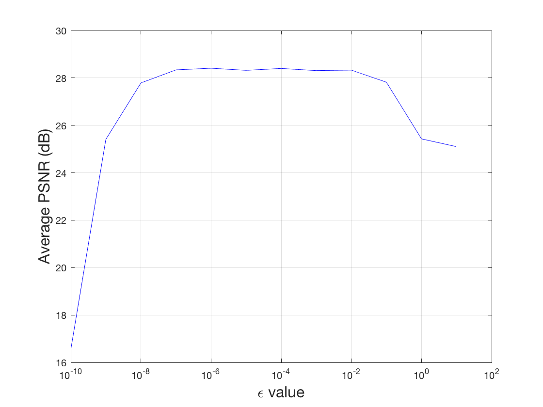
Figure 2: Performance of SDA-SURE for different $\epsilon$ values at $\sigma=25$.

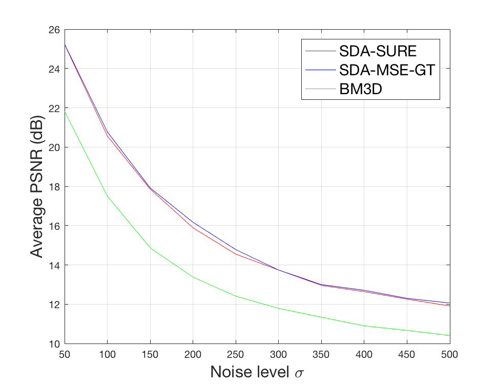
Figure 3: Performance of denoising methods at different $\sigma$ values.

The accuracy of MC-SURE also depends on the noise level $\sigma$. It was observed that the SURE loss curves become noisier compared to MSE loss curves as $\sigma$ increases. However, they still followed similar trends and yielded similar average PSNRs on MNIST dataset as shown in Fig. 3. We observed that after $\sigma=350$, SURE loss curves started to become too noisy and thus deviated from the trends of their corresponding MSE loss curves. Conversely, noise levels $\sigma>300$ were too high for both SDA-based denoisers and BM3D, so that they were not able to output recognizable digits. Therefore, SDA-SURE can be trained effectively on adequately high noise levels so that it can yield a performance that is comparable to SDA-MSE-GT and can consistently outperform BM3D.

TABLE III: Results of denoising methods on 12 widely used images (Set12 dataset) (Performance in dB).

Image	C.Man	House	Peppers	Starfish	Monar.	Airpl.	Parrot	Lena	Barbara	Boat	Man	Couple	Average
$\sigma=25$
BM3D	29.47	33.00	30.23	28.58	29.35	28.37	28.89	32.06	30.64	29.78	29.60	29.70	29.97
DnCNN-BM3D	29.34	31.99	30.13	28.38	29.21	28.46	28.91	31.53	28.89	29.6	29.52	29.54	29.63
DnCNN-SURE	29.80	32.70	30.58	29.08	30.11	28.94	29.17	32.06	29.16	29.84	29.89	29.76	30.09
DnCNN-MSE-GT	30.14	33.16	30.84	29.4	30.45	29.11	29.36	32.44	29.91	30.11	30.08	30.06	30.42
$\sigma=50$
BM3D	26.00	29.51	26.58	25.01	25.78	25.15	25.98	28.93	27.19	26.62	26.79	26.46	26.67
DnCNN-BM3D	25.76	28.43	26.5	24.9	25.66	25.15	25.82	28.36	25.3	26.5	26.6	26.17	26.26
DnCNN-SURE	26.48	29.14	26.77	25.38	26.50	25.66	26.21	28.79	24.86	26.78	26.97	26.51	26.67
DnCNN-MSE-GT	27.03	29.92	27.27	25.65	26.95	25.93	26.43	29.31	26.17	27.12	27.22	26.94	27.16
$\sigma=75$
BM3D	24.58	27.45	24.69	23.19	23.81	23.38	24.22	27.14	25.08	25.05	25.30	24.73	24.89
DnCNN-BM3D	24.11	27.02	24.48	23.09	23.73	23.40	24.06	27.11	23.80	24.84	25.19	24.59	24.62
DnCNN-SURE	24.65	27.16	24.49	23.25	24.10	23.52	24.13	26.92	23.02	25.09	25.37	24.70	24.70
DnCNN-MSE-GT	25.46	28.04	25.22	23.62	24.81	23.97	24.71	27.60	23.88	25.53	25.68	25.13	25.30

4.4 Results: high resolution natural images dataset

To demonstrate the capabilities of our SURE-based deep learning denoisers, we investigated a deeper and more powerful denoising network called DnCNN [16] using high resolution images. DnCNN consisted of 17 layers of CNN with batch normalization and ReLU activation functions. Each convolutional layer had 64 filters with sizes of $3\times 3$. Similar to [16], the network was trained with 400 images with matrix sizes of $180\times 180$ pixels. In total, $1772\times 128$ image patches with sizes of $40\times 40$ pixels were extracted randomly from these images. Two test sets were used to evaluate performance: one set consisted of 12 widely used images (Set12) [27], and the other was a BSD68 dataset. For all cases, the network was trained with 50 epochs using the Adam optimization algorithm with an initial learning rate of $10^{-3}$, which eventually decayed to $10^{-4}$ after 40 epochs. The batch size was set to 128 (note that bigger batch sizes did not improve performance). Images were corrupted at three noise levels ($\sigma$ = 25, 50, 75).

DnCNN used residual learning whereby the network was forced to learn the difference between noisy and ground truth images. The output residual image was then subtracted from the input noisy image to yield the estimated image. Thus, our network was trained with SURE as

$$\boldsymbol{h}(\boldsymbol{y};{\boldsymbol{\theta}})=\boldsymbol{y}-\boldsymbol{\mathrm{CNN}}_{{\boldsymbol{\theta}}}(\boldsymbol{y})$$ (17)

where $\boldsymbol{\mathrm{CNN}}_{{\boldsymbol{\theta}}}(.)$ is the DnCNN that is being trained using residual learning. For DnCNN, selecting an appropriate $\epsilon$ value in (4) turned out to be important for a good denoising performance. To achieve stable training with good performance, $\epsilon$ had to be tuned for each of the chosen noise levels of $\sigma$ = 25, 50, 75. We observed that the optimal value for $\epsilon$ was proportional to $\sigma$ as shown in [41]. All the experiments were performed with the setting of

$$\epsilon=\sigma\times 1.4\times 10^{-4}.$$ (18)

With the use of an NVidia Titan X GPU, the training process took approximately 7 hours for DnCNN-MSE-GT and approximately 11 hours for DnCNN-SURE. SURE based methods took more training time than MSE based methods because of the additional divergence calculations executed to optimize the MC-SURE cost function.

TABLE IV: Results of denoising methods on BSD68 dataset (Performance in dB).

Methods	BM3D	DnCNN-BM3D	DnCNN-SURE	DnCNN-MSE-GT
$\sigma=25$	28.56	28.54	28.97	29.20
$\sigma=50$	25.62	25.44	25.93	26.22
$\sigma=75$	24.20	24.09	24.31	24.66

Tables III and IV present denoising performance results using (a) the BM3D denoiser [27], (b) a state-of-the-art deep CNN (DnCNN) image denoiser trained with MSE [16], and (c) the same DnCNN image denoiser trained with SURE without the use of noiseless ground truth images. The MSE-based DnCNN image denoiser with ground truth data, DnCNN-MSE-GT, yielded the best denoising performance compared to other methods, such as the BM3D, which is consistent with the results in [16].

As seen in Table III, for the Set12 dataset, SURE-based denoisers achieved performances comparable to or better than that for BM3D for noise levels $\sigma=25$ and $50$. In contrast, for a higher noise level ($\sigma=75$), DnCNN-SURE yielded lower average PSNR value by 0.19 dB than BM3D. BM3D had exceptionally good denoising performance on the “Barbara” image (up to 2.33 dB better PSNR), and even outperformed the DnCNN-MSE-GT method. In the case of the BSD68 dataset in Table IV, the SURE-based method outperformed BM3D for all the noise levels. Unlike the case of Set12, we observed that DnCNN-SURE yielded significantly better performance than BM3D, and yielded increased average PSNR values by 0.11-0.41 dB.

Differences among the performances of denoisers in Tables III and IV can be explained by the working principle of BM3D. Since BM3D looks for similar image patches for denoising, repeated patterns (as in the “Barbara” image) and flat areas (as in “House” image) can be key factors to generating improved denoising results. One of the advantages of DnCNN-SURE over BM3D is that it does not suffer from rare patch effects. If the test image is relatively detailed and does not contain many repeated patterns, BM3D will have poorer performance than the proposed DnCNN-SURE method. Note that the DnCNN-BM3D method that trains networks by optimizing MSE with BM3D denoised images as the ground truth yielded slightly worse performance than the BM3D itself (Tables III, IV).

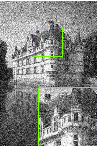
(a) Noisy image / 14.76dB

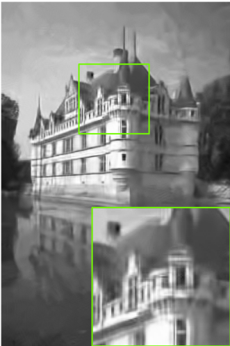
(b) BM3D / 26.14dB

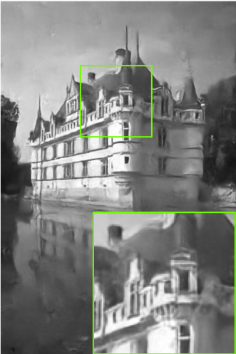
(c) DnCNN-SURE / 26.46dB

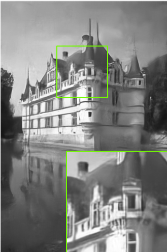
(d) DnCNN-MSE-GT / 26.85dB

Figure 4: Denoising results of an image from the BSD68 dataset for $\sigma=50$.

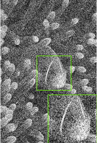
(a) Noisy image / 11.77dB

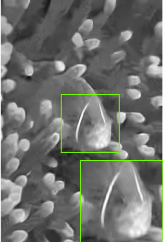
(b) BM3D / 26.21dB

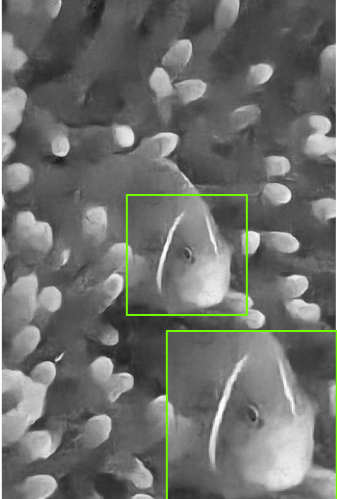
(c) DnCNN-SURE / 26.46dB

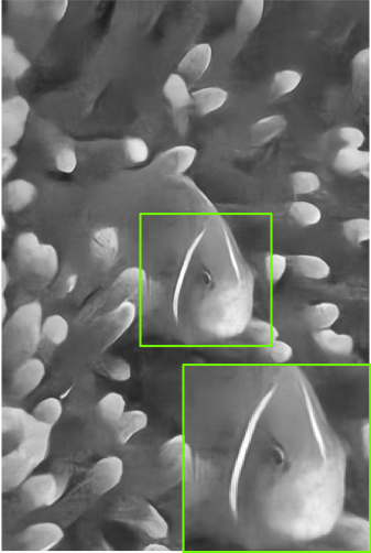
(d) DnCNN-MSE-GT / 27.10dB

Figure 5: Denoising results of an image from the BSD68 dataset for $\sigma=75$.

Fig. 4 illustrates the denoised results for an image from the BSD68 dataset. Visual quality assessment indicated that BM3D yielded blurrier images and thus yielded worse PSNR compared to the results generated by DNN denoisers. DnCNN-SURE effectively removed noise while preserving edges to yield sharper images. DnCNN-MSE-GT had the best denoised image with the highest PSNR of 26.85 dB. In Fig. 5, an image from the BSD68 dataset is contaminated with severe noise ($\sigma=75$). BM3D struggled to preserve important details in the image such as the outline of the fish’s eye, while DnCNN-SURE yielded much sharper image with higher PSNR.

4.5 Extension to blind color image denoising

We adopted the CDnCNN network from [16] for blind color denoising and incorporated our SURE-based training by minimizing (14). Following [16], the network consisted of 20 layers and was trained with 432 colored images. In total, $3000\times 128$ image patches with sizes of $50\times 50$ were randomly extracted from these images. We trained a single CDnCNN network for the noise levels of $\sigma=\left[0,55\right]$. The experiments were performed setting $\epsilon^{(j)}=\sigma^{(j)}\times 1.2\times 10^{-4}$. All the other simulation details were the same as the ones for grayscale denoising in Section 4.4.

TABLE V: Results of denoising methods on CBSD68 dataset (Performance in dB).

Methods	CBM3D	CDnCNN-SURE	CDnCNN-MSE-GT
$\sigma=25$	30.70	31.06	31.21
$\sigma=50$	27.38	27.75	27.96

(a) Noisy image / 14.67dB

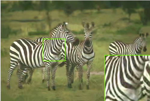
(b) CBM3D / 26.47dB

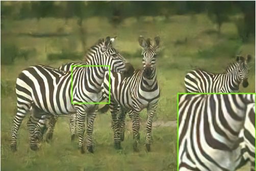
(c) CDnCNN-SURE / 27.28dB

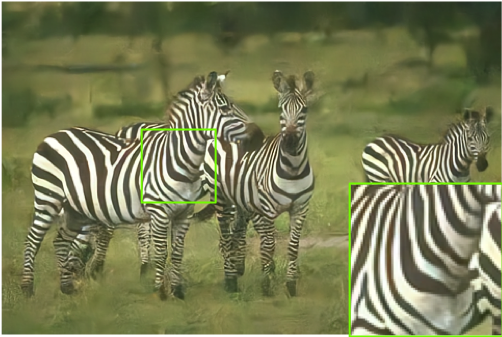
(d) CDnCNN-MSE-GT / 27.47dB

Figure 6: Denoising results of an image from the CBSD68 dataset for $\sigma=50$.

TABLE VI: Results of denoising methods on 9 widely used color images (Performance in dB). * indicates instances where SURE-FT outperformed MSE-GT.

Image	House	Peppers	Lena	Baboon	F16	Kodak1	Kodak2	Kodak3	Kodak12	Average
$\sigma=25$
CBM3D	33.02	31.23	32.27	25.95	32.76	29.17	32.44	34.61	33.76	31.69
DIP	31.75	29.09	30.50	22.67	31.56	25.21	30.39	30.56	30.71	29.16
CDnCNN-SURE	31.06	30.35	31.88	25.53	31.68	29.54	32.56	34.42	33.70	31.19
CDnCNN-SURE-FT	32.69*	31.35*	32.45*	26.47*	33.30*	29.77*	32.90*	34.72	33.94	31.95*
CDnCNN-MSE-GT	31.47	30.67	32.13	25.82	31.95	29.64	32.83	34.77	33.98	31.47
$\sigma=50$
CBM3D	30.54	28.97	29.90	23.14	29.76	25.90	29.89	31.43	30.98	28.95
DIP	28.39	26.98	28.41	21.21	27.79	23.96	27.52	28.09	27.63	26.66
CDnCNN-SURE	29.01	28.29	29.44	23.21	28.99	26.29	29.76	31.19	30.79	28.55
CDnCNN-SURE-FT	29.95*	29.03*	29.86*	23.64*	30.14*	26.50*	30.09	31.43	30.92	29.06*
CDnCNN-MSE-GT	29.57	28.69	29.74	23.40	29.36	26.45	30.21	31.66	31.19	28.92

Table V presents denoising performance on CBSD68 dataset using (a) the CBM3D denoiser [27], (b) CDnCNN image denoiser trained with MSE [16], and (c) the same CDnCNN image denoiser trained with SURE without the use of noiseless ground truth images. Both deep learning methods outperformed the conventional method CBM3D method by a large margin. This is consistent with the results of DnCNN methods on the grayscale BSD68 dataset. Even though color blind image denoising is a harder task than grayscale non-blind single noise level denoising, CDnCNN-SURE showed a superior denoising performance compared to the CBM3D. This illustrates the powerful capabilities of the SURE-based optimization for extended settings such as multiple noise levels and color images.

Fig. 6 illustrates the denoised results for an image from CBSD68 dataset that was contaminated at the noise level of $\sigma=50$. Both deep learning methods yielded higher quality images compared to the CBM3D. The denoised image CBM3D contained false color artifacts whereas CDnCNN methods preserved the true colors and fine details.

4.6 Unsupervised refining (fine-tuning) with SURE

Since our SURE-based training method does not require the ground truth images, we can utilize noisy test images to train the deep neural networks. One way to execute this could be just adding the noisy test images to the training datasets and train the network from scratch [33]. However, this method is slow and requires retraining the network for the future test sets. We propose a more practical and faster method called SURE-FT in which we fine-tune a pretrained denoising network on a noisy test image by minimizing (15).

To demonstrate the effectiveness of this method, we took CDnCNN-SURE from Section 4.5 as a baseline denoiser network and fine-tuned it on an individual noisy image (CDnCNN-SURE-FT) for all test images. Our proposed fine-tuning process is different from the original training process. Firstly, we used a single test image without dividing it into small patches for each fine-tuning. Secondly, we froze batch normalization layers in CDnCNN because of the change of the dataset size. The initial learning rate was set to $10^{-4}$ and the network was fine-tuned for 75 epochs (learning rate was decayed to $5\times 10^{-5}$ after 50 epochs). For each image, it took about 24.5, 75.25, 123.75 seconds per image (256 $\times$ 256, 512 $\times$ 512, , 768 $\times$ 512), respectively, for 75 epochs.

The methods are evaluated on 9 widely used color images [49] and CDnCNN-SURE-FT was implemented for each image separately. We additionally report the performance of deep image prior method (DIP) [32], which also optimizes DNNs using the input noisy image only. We used the official PyTorch implementation from the authors and took the hyperparameters from the paper [32].

Table VI demonstrates the performance of various denoising methods. Unlike the CBSD68 dataset, CBM3D has superior performance to both CDnCNN-SURE and CDnCNN-MSE-GT methods on most of the color images. The structure of these test images are quite different from the 432 training images and some contain many repeated patterns and flat areas which are favorable for CBM3D. This is where fine-tuning on the noisy test images can provide its benefits. Our proposed CDnCNN-SURE-FT vastly improved the performance over the CDnCNN-SURE on almost all of the test images, often by more than 1dB gain in some images. This shows that the network could learn the unique patterns and details from the noisy test images and denoised them effectively. As a result, CDnCNN-SURE-FT outperformed all the other methods on both noise levels, including CBM3D, CDnCNN-MSE-GT in many images and on average (indicated with *). The DIP method had the worst performance, falling behind the CDnCNN-SURE method by almost 2dB.

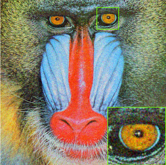
(a) Noisy image / 20.34dB

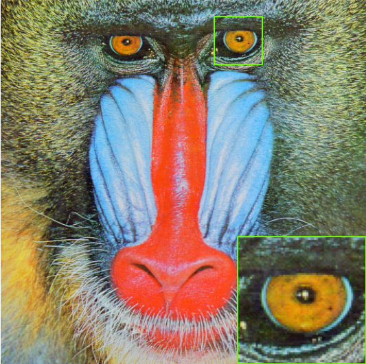
(b) Ground truth

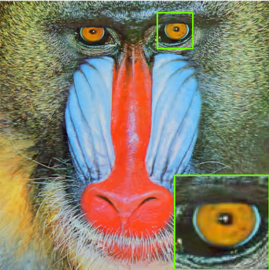
(c) CBM3D / 29.89dB

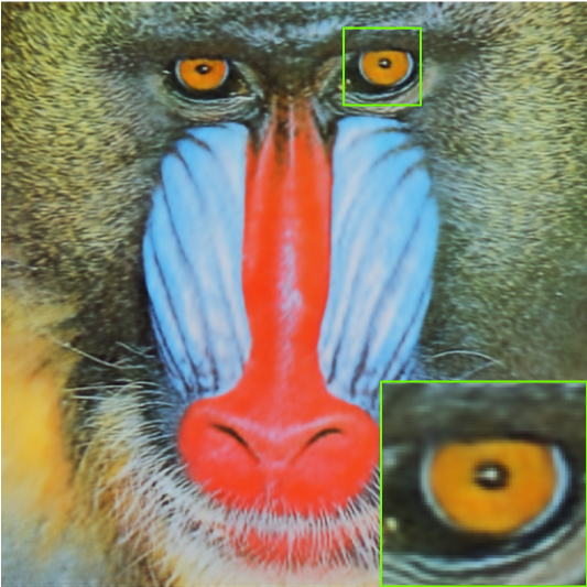
(d) DIP / 27.52dB

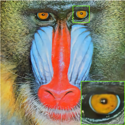
(e) CDnCNN-SURE / 29.76dB

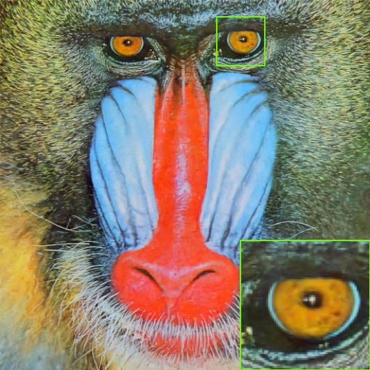
(f) CDnCNN-SURE-FT / 30.09dB

Figure 7: Denoising results of the “Baboon” image for $\sigma=25$.

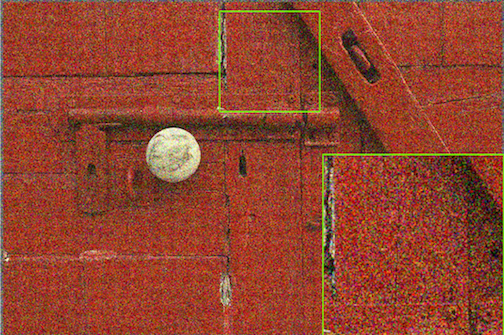
(a) Noisy image / 15.21dB

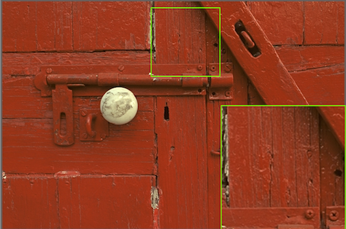
(b) Ground Truth

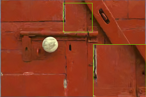
(c) CBM3D / 32.27dB

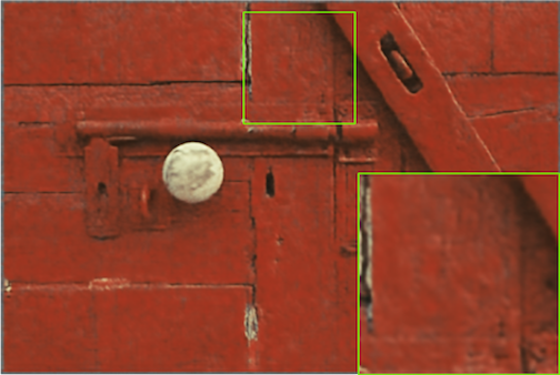
(d) DIP / 30.50dB

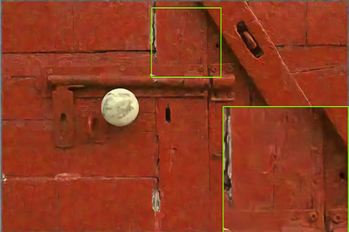
(e) CDnCNN-SURE / 31.88dB

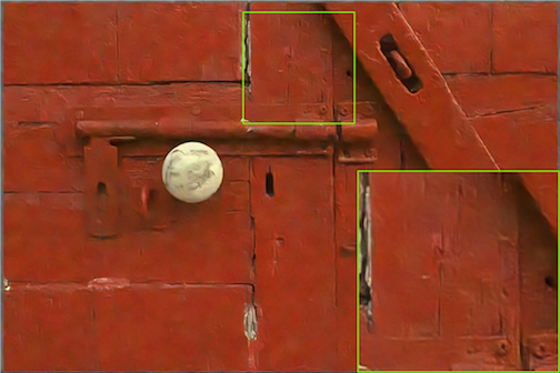
(f) CDnCNN-SURE-FT / 32.45dB

Figure 8: Denoising results of the “Kodak 2” image for $\sigma=50$.

(a) Noisy

(b) BM3D+VST

(c) SDA-PURE

(d) SDA-MSE-GT

Figure 9: Denoising results of SDA with various methods for MNIST dataset for $\zeta=0.1$.

(a) Noisy

(b) BM3D+VST

(c) SDA-PURE

(d) SDA-MSE-GT

Figure 10: Denoising results of SDA with various methods for MNIST dataset for $\zeta=0.2$.

Fig. 7 illustrates the denoised results of the “Baboon” image at $\sigma=25$. The eye region is good for the comparison of the methods. We can see that CBM3D had slightly better details and quantitative performance than CDnCNN-SURE, while DIP image was relatively blurry. Our proposed CDnCNN-SURE-FT yielded a sharper image which was closer to the ground truth image visually and quantitatively. In Fig. 8, all methods were evaluated on the “Kodak 2” image that was contaminated with the noise level of $\sigma=50$. CDnCNN-SURE image seemed to preserve more details than CBM3D (bottom right), however contained artifacts throughout the entire image. Our CDnCNN-SURE-FT got rid of most artifacts and yielded cleaner image. Moreover, the denoised image contained more details than CBM3D and was closer to the ground truth. The DIP yielded blurry and low quality image.

4.7 Extension to Poisson noise denoising

We performed Poisson denoising simulations with the MNIST dataset with the same SDA network as in Section 4.1. For the comparison, we chose the conventional BM3D+VST method [50] that uses the optimal Anscombe transformation. Table VII shows that for $\zeta=0.01$, all methods had similar performance in terms of average PSNR. However, for higher $\zeta=0.1,0.2$ values (higher noise), our proposed SDA-PURE method outperformed the conventional BM3D+VST method significantly, while SDA-MSE-GT that was trained with the ground truth data yielded the best results. Figs. 9 and 10 illustrate the visual quality of the outputs of the denoising methods for $\zeta=0.1$ and $0.2$, respectively. We observed that BM3D+VST images were considerably blurrier than the results of our SDA-based methods, especially for $\zeta=0.2$.

It was found that for $\dot{\epsilon}$ in the range of $\left[10^{-6},10^{-2}\right]$ worked well for PURE approximation, which is similar to the SURE case. At high values of $\zeta>0.1$, the approximation became highly inaccurate and after $\zeta>0.2$ the model could not converge and thus training was not feasible. These findings about the accuracy of PURE approximation are in agreement with [48].

TABLE VII: Results of Poisson noise denoisers for MNIST (Performance in dB). Averages of 10 experiments are reported.

Methods	BM3D+VST	SDA-PURE	SDA-MSE-GT
$\zeta=0.01$	30.57	30.55	30.55
$\zeta=0.1$	22.34	25.80	25.99
$\zeta=0.2$	19.56	23.51	24.27

5 Discussion

Our proposed SURE-based DNN denoisers can be useful for the applications with large amounts of noisy images, but with few noiseless images. Note that we proposed method to train and refine DNN denoisers in unsupervised ways rather than the denoiser network itself. Since deep learning based denoising research for novel DNN architectures is still evolving, incorporating our proposed SURE and SURE-FT methods into these new high performance DNN denoiser networks could possibly to achieve significantly better performances than BM3D, or other conventional state-of-the-art denoisers. Further investigation will be needed for high performance denoising networks for synthetic and real noise.

Our proposed SURE-FT method looks similar to recently proposed DIP [32] in terms of training (or refining) a DNN network for a given test image. While DIP has a wide variety of applications such as denoising, super resolution, inpainting, and reconstruction, our SURE-FT is restricted to Gaussian denoising. However, as shown in this article, our proposed SURE-FT yielded significantly better performance than DIP for Gaussian noise removal. SURE-FT can be applied to refine many existing, pretrained deep learning based denoisers, while DIP requires special network architecture such as U-Net [51] to achieve high performance. We also tried to train a network from scratch with SURE-FT (i.e. with a single noisy test image) that is similar to DIP, but that network was not able to yield good denoised performance. Thus, it seems important to apply SURE-FT to pretrained networks such as CDnCNN-SURE to benefit from the information provided by large training dataset. In other words, our SURE-FT combines both the state-of-the-art deep learning based denoising and learning to denoise the unique structures of an input image.

In this work, Gaussian with known $\sigma$ and Poisson noise with known $\zeta$ was assumed in all simulations. However, there are several methods to estimate those parameters that can be used with our methods (see [40] and  [48] for details). SURE can incorporate a variety of noise distributions other than Gaussian noise. Generalized SURE for exponential families has been proposed [52] so that other common noise types in imaging systems can be potentially considered for SURE-based methods. It should be noted that SURE does not require any prior knowledge on images. Thus, it can be applied to the measurement domain for different applications, such as medical imaging. Owing to noise correlation (colored noise) in the image domain (e.g., based on the Radon transform in the case of CT or PET), further investigations will be necessary to apply our proposed method directly to the image domain.

Note that unlike (5), the existence of the minimizer for (13) should be considered with care since it is theoretically possible that (13) becomes negative infinity due to the divergence term in (13). However, in practice, this issue can be addressed by introducing a regularizer (weight decay), with a DNN structure so that denoisers can impose regularity conditions on the function $h$ (e.g., bounded norm of $\nabla h$), either by choosing an adequate $\epsilon$ value, or by using proper training data. Lastly, note that we derived (13), an unbiased estimator for MSE, assuming a fixed $\boldsymbol{\theta}$. Thus, there is no guarantee that the resulting estimator (denoiser) that is tuned by SURE will be unbiased [53].

6 Conclusion

We proposed a SURE based training method for general deep learning denoisers in unsupervised ways. Our proposed method with SURE trained DNN denoisers without noiseless ground truth data so that they could yield comparable denoising performances to those elicited by the same denoisers that were trained with noiseless ground truth data, and outperform the conventional state-of-the-art BM3D. Our proposed SURE-based refining method with a noisy test image further improved performance and outperformed conventional BM3D, deep image prior, and often the networks trained with ground truth for both grayscale and color images. Potential extension of our SURE-based methods to Poisson noise model was also demonstrated.

References

- [1] A. Krizhevsky, I. Sutskever, and G. E. Hinton, “Imagenet classification with deep convolutional neural networks,” in Advances in Neural Information Processing Systems (NIPS) 25, 2012, pp. 1097–1105.
- [2] K. He, X. Zhang, S. Ren, and J. Sun, “Deep Residual Learning for Image Recognition,” in IEEE Conference on Computer Vision and Pattern Recognition (CVPR), 2016, pp. 770–778.
- [3] C. Szegedy, S. Ioffe, V. Vanhoucke, and A. A. Alemi, “Inception-v4, Inception-ResNet and the Impact of Residual Connections on Learning.” in AAAI Conference on Artificial Intelligence (AAAI), 2017, pp. 4278–4284.
- [4] R. Girshick, J. Donahue, and T. Darrell, “Rich feature hierarchies for accurate object detection and semantic segmentation,” in IEEE Conference on Computer Vision and Pattern Recognition (CVPR), 2014, pp. 580–587.
- [5] S. Ren, K. He, R. Girshick, and J. Sun, “Faster R-CNN: Towards real-time object detection with region proposal networks,” in Advances in Neural Information Processing Systems (NIPS) 28, 2015, pp. 91–99.
- [6] J. Redmon and A. Farhadi, “YOLO9000: Better, Faster, Stronger,” in IEEE Conference on Computer Vision and Pattern Recognition (CVPR). IEEE, Jul. 2017, pp. 6517–6525.
- [7] L.-C. Chen, G. Papandreou, I. Kokkinos, K. Murphy, and A. L. Yuille, “Semantic image segmentation with deep convolutional nets and fully connected crfs,” in International Conference on Learning Representation (ICLR), 2015.
- [8] J. Long, E. Shelhamer, and T. Darrell, “Fully convolutional networks for semantic segmentation,” in IEEE Conference on Computer Vision and Pattern Recognition (CVPR), 2015, pp. 3431–3440.
- [9] L.-C. Chen, Y. Zhu, G. Papandreou, F. Schroff, and H. Adam, “Encoder-Decoder with Atrous Separable Convolution for Semantic Image Segmentation,” in European Conference on Computer Vision (ECCV). Springer International Publishing, 2018, pp. 833–851.
- [10] I. Goodfellow, J. Pouget-Abadie, M. Mirza, B. Xu, D. Warde-Farley, S. Ozair, A. Courville, and Y. Bengio, “Generative Adversarial Nets,” in Advances in Neural Information Processing Systems (NIPS), 2014, pp. 2672–2680.
- [11] D. P. Kingma and M. Welling, “Auto-Encoding Variational Bayes,” in International Conference on Learning Representations (ICLR), 2014.
- [12] J.-Y. Zhu, T. Park, P. Isola, and A. A. Efros, “Unpaired Image-to-Image Translation Using Cycle-Consistent Adversarial Networks,” in IEEE International Conference on Computer Vision (ICCV). IEEE, 2017, pp. 2242–2251.
- [13] P. Vincent, H. Larochelle, I. Lajoie, Y. Bengio, and P. A. Manzagol, “Stacked denoising autoencoders: Learning Useful Representations in a Deep Network with a Local Denoising Criterion,” Journal of Machine Learning Research, vol. 11, pp. 3371–3408, Dec. 2010.
- [14] H. C. Burger, C. J. Schuler, and S. Harmeling, “Image denoising: Can plain neural networks compete with BM3D?” in IEEE Conference on Computer Vision and Pattern Recognition (CVPR), 2012, pp. 2392–2399.
- [15] Y.-Q. Wang and J.-M. Morel, “Can a Single Image Denoising Neural Network Handle All Levels of Gaussian Noise?” IEEE Signal Processing Letters, vol. 21, no. 9, pp. 1150–1153, May 2014.
- [16] K. Zhang, W. Zuo, Y. Chen, D. Meng, and L. Zhang, “Beyond a Gaussian Denoiser: Residual Learning of Deep CNN for Image Denoising,” IEEE Transactions on Image Processing, vol. 26, no. 7, pp. 3142–3155, May 2017.
- [17] S. Lefkimmiatis, “Non-local Color Image Denoising with Convolutional Neural Networks,” in IEEE Conference on Computer Vision and Pattern Recognition (CVPR), 2017, pp. 5882–5891.
- [18] J. Xie, L. Xu, and E. Chen, “Image denoising and inpainting with deep neural networks,” in Advances in Neural Information Processing Systems (NIPS) 25, 2012, pp. 341–349.
- [19] S. Iizuka, E. Simo-Serra, and H. Ishikawa, “Globally and locally consistent image completion,” ACM Transactions on Graphics, vol. 36, no. 4, pp. 1–14, Jul. 2017.
- [20] R. A. Yeh, C. Chen, T. Yian Lim, A. G. Schwing, M. Hasegawa-Johnson, and M. N. Do, “Semantic image inpainting with deep generative models,” in IEEE Conference on Computer Vision and Pattern Recognition (CVPR). IEEE, 2017, pp. 6882–6890.
- [21] C. Dong, C. C. Loy, K. He, and X. Tang, “Image super-resolution using deep convolutional networks,” IEEE transactions on pattern analysis and machine intelligence, vol. 38, no. 2, pp. 295–307, 2016.
- [22] B. Lim, S. Son, H. Kim, S. Nah, and K. M. Lee, “Enhanced Deep Residual Networks for Single Image Super-Resolution,” in IEEE Conference on Computer Vision and Pattern Recognition Workshops (CVPRW). IEEE, 2017, pp. 1132–1140.
- [23] D. Park, K. Kim, and S. Y. Chun, “Efficient module based single image super resolution for multiple problems,” in IEEE Conference on Computer Vision and Pattern Recognition Workshops (CVPRW), Ulsan National Institute of Science and Technology, Ulsan, South Korea. IEEE, 2018, pp. 995–1003.
- [24] X. J. Mao, C. Shen, and Y. B. Yang, “Image restoration using very deep convolutional encoder-decoder networks with symmetric skip connections,” in Advances in Neural Information Processing Systems (NIPS) 29, 2016, pp. 2810–2818.
- [25] R. Gao and K. Grauman, “On-demand learning for deep image restoration,” in IEEE International Conference on Computer Vision (ICCV), 2017.
- [26] K. Zhang, W. Zuo, S. Gu, and L. Zhang, “Learning Deep CNN Denoiser Prior for Image Restoration,” in IEEE Conference on Computer Vision and Pattern Recognition (CVPR), 2017, pp. 3929–3938.
- [27] K. Dabov, A. Foi, V. Katkovnik, and K. Egiazarian, “Image denoising by sparse 3-D transform-domain collaborative filtering,” IEEE Transactions on Image Processing, vol. 16, no. 8, pp. 2080–2095, Aug. 2007.
- [28] M. Ye, Y. Qian, and J. Zhou, “Multitask Sparse Nonnegative Matrix Factorization for Joint Spectral–Spatial Hyperspectral Imagery Denoising,” IEEE Transactions on Geoscience and Remote Sensing, vol. 53, no. 5, pp. 2621–2639, Dec. 2014.
- [29] H. Chen, Y. Zhang, M. K. Kalra, F. Lin, Y. Chen, P. Liao, J. Zhou, and G. Wang, “Low-Dose CT With a Residual Encoder-Decoder Convolutional Neural Network,” IEEE Transactions on Medical Imaging, vol. 36, no. 12, pp. 2524–2535, Nov. 2017.
- [30] E. Kang, J. Min, and J. C. Ye, “A deep convolutional neural network using directional wavelets for low-dose X-ray CT reconstruction,” Medical Physics, vol. 44, no. 10, pp. e360–e375, Oct. 2017.
- [31] J. Lehtinen, J. Munkberg, J. Hasselgren, S. Laine, T. Karras, M. Aittala, and T. Aila, “Noise2Noise: Learning Image Restoration without Clean Data,” in International Conference on Machine Learning (ICML), 2018, pp. 2965–2974.
- [32] D. Ulyanov, A. Vedaldi, and V. Lempitsky, “Deep Image Prior,” in IEEE Conference on Computer Vision and Pattern Recognition (CVPR), 2018, pp. 9446–9454.
- [33] S. Soltanayev and S. Y. Chun, “Training deep learning based denoisers without ground truth data,” in Advances in Neural Information Processing Systems 31, 2018, pp. 3261–3271.
- [34] C. M. Stein, “Estimation of the mean of a multivariate normal distribution,” The Annals of Statistics, vol. 9, no. 6, pp. 1135–1151, Nov. 1981.
- [35] D. L. Donoho and I. M. Johnstone, “Adapting to unknown smoothness via wavelet shrinkage,” Journal of the american statistical association, vol. 90, no. 432, pp. 1200–1224, 1995.
- [36] X.-P. Zhang and M. D. Desai, “Adaptive denoising based on sure risk,” IEEE signal processing letters, vol. 5, no. 10, pp. 265–267, 1998.
- [37] D. Van De Ville and M. Kocher, “SURE-Based Non-Local Means,” IEEE Signal Processing Letters, vol. 16, no. 11, pp. 973–976, Nov. 2009.
- [38] J. Salmon, “On Two Parameters for Denoising With Non-Local Means,” IEEE Signal Processing Letters, vol. 17, no. 3, pp. 269–272, Mar. 2010.
- [39] M. P. Nguyen and S. Y. Chun, “Bounded Self-Weights Estimation Method for Non-Local Means Image Denoising Using Minimax Estimators,” IEEE Transactions on Image Processing, vol. 26, no. 4, pp. 1637–1649, Feb. 2017.
- [40] S. Ramani, T. Blu, and M. Unser, “Monte-Carlo Sure: A Black-Box Optimization of Regularization Parameters for General Denoising Algorithms,” IEEE Transactions on Image Processing, vol. 17, no. 9, pp. 1540–1554, Aug. 2008.
- [41] C.-A. Deledalle, S. Vaiter, J. Fadili, and G. Peyré, “Stein unbiased gradient estimator of the risk (sugar) for multiple parameter selection,” SIAM Journal on Imaging Sciences, vol. 7, no. 4, pp. 2448–2487, 2014.
- [42] T. Blu and F. Luisier, “The SURE-LET Approach to Image Denoising,” IEEE Transactions on Image Processing, vol. 16, no. 11, pp. 2778–2786, Oct. 2007.
- [43] L. Bottou, “Online Learning and Stochastic Approximations,” in On-line learning in neural networks. Cambridge University Press New York, NY, USA, 1998, pp. 9–42.
- [44] Y. Nesterov, “A method of solving a convex programming problem with convergence rate o (1/k2),” in Soviet Mathematics Doklady, 1983.
- [45] D. P. Kingma and J. Ba, “Adam - A Method for Stochastic Optimization,” in International Conference on Learning Representation (ICLR), 2015.
- [46] M. Abadi et al., “Tensorflow: A system for large-scale machine learning,” in Proceedings of the 12th USENIX Conference on Operating Systems Design and Implementation, 2016, pp. 265–283.
- [47] F. Luisier, T. Blu, and M. Unser, “Image denoising in mixed poisson–gaussian noise,” IEEE Transactions on image processing, vol. 20, no. 3, pp. 696–708, 2011.
- [48] Y. Le Montagner, E. D. Angelini, and J.-C. Olivo-Marin, “An unbiased risk estimator for image denoising in the presence of mixed poisson–gaussian noise,” IEEE Transactions on Image Processing, vol. 23, no. 3, pp. 1255–1268, 2014.
- [49] A. Foi, “Image and video denoising by sparse 3d transform-domain collaborative filtering block-matching and 3d filtering (bm3d) algorithm and its extensions.” [Online]. Available: http://www.cs.tut.fi/~foi/GCF-BM3D/index.html#ref_results
- [50] M. Makitalo and A. Foi, “Optimal inversion of the anscombe transformation in low-count poisson image denoising,” IEEE transactions on Image Processing, vol. 20, no. 1, pp. 99–109, 2011.
- [51] O. Ronneberger, P. Fischer, and T. Brox, “U-Net: Convolutional Networks for Biomedical Image Segmentation,” in International Conference on Medical Image Computing and Computer-Assisted Intervention (MICCAI), 2015, pp. 234–241.
- [52] Y. C. Eldar, “Generalized SURE for Exponential Families: Applications to Regularization,” IEEE Transactions on Signal Processing, vol. 57, no. 2, pp. 471–481, Jan. 2009.
- [53] R. J. Tibshirani and S. Rosset, “Excess optimism: How biased is the apparent error of an estimator tuned by sure?” arXiv preprint arXiv:1612.09415, 2016.