Computational Results for the Higgs Boson Equation in the de Sitter Spacetime
Abstract
High performance computations are presented for the Higgs Boson Equation in the de Sitter Spacetime using explicit fourth order Runge-Kutta scheme on the temporal discretization and fourth order finite difference discretization in space. In addition to the fully three space dimensional equation its one space dimensional radial solutions are also examined. The numerical code for the three space dimensional equation has been programmed in CUDA Fortran and was performed on NVIDIA Tesla K40c GPU Accelerator. The radial form of the equation was simulated in MATLAB. The numerical results demonstrate the existing theoretical result that under certain conditions bubbles form in the scalar field. We also demonstrate the known blow-up phenomena for the solutions of the semilinear Klein-Gordon equation with imaginary mass. Our numerical studies suggest several previously not known properties of the solution for which theoretical proofs do not exist yet: 1. smooth solution exists for all time if the initial conditions are compactly supported and smooth; 2. under some conditions no bubbles form; 3. solutions converge to step functions related to unforced, damped Duffing equations.
The University of Texas Rio Grande Valley, Edinburg TX, 78539, United States
Keywords — Higgs boson equation in the de Sitter spacetime, High-performance computation, Unforced damped Duffing equations
1 Introduction
There are several open mathematical questions about the Higgs boson in the de Sitter spacetime. We are interested in the feature of this issue related to the partial differential equations theory and, especially, to the problem of the global in time existence of the solution. In fact, the equation is semilinear since it contains the Higgs potential and has time dependent coefficient. Because of the lack of mathematically rigorous proof of the existence of global in time solution we turn to numerical investigations which can shed a light on that issue, and also to indicate the creation of so-called bubbles. In order to achieve that aim, in this article we perform high-performance numerical computations using Graphical Processing Units for examining the behavior of solutions to the Higgs boson equation in the de Sitter spacetime.
The Klein-Gordon equation with the Higgs potential (the Higgs boson equation) in the de Sitter spacetime can be written as
| (1.1) | ||||
| (1.2) | ||||
| (1.3) |
Here is the Laplace operator in , is the time variable, the parameters are and , while is a real-valued function. From now on we consider solution to the Klein-Gordon equation which is at least continuous. It is of considerable interest for particle physics and inflationary cosmology to study the so-called bubbles [7, 19, 26]. In the quantum field theory a bubble is defined as a simply connected domain surrounded by a wall such that the field approaches one of the vacuums outside of a bubble (see, e.g., [7]). It is mathematically reasonable to define the bubble as a maximal connected set of spatial points at which solution to the Cauchy problem (1.1)–(1.3) changes sign.
First we discuss the existence of global in time solution of equations (1.1)–(1.3) and of the more general equation
| (1.4) |
where or , or some more general function, and . For this equation the local existence of solution in different spaces of functions is well investigated for appropriate values of and . The estimate for the lifespan of the solution is given as follows. The main parameter that controls estimates and solvability is the principal square root . The following result is from Theorem 0.1 in [29].
Let be the usual Sobolev space [1]. The function is said to be Lipschitz continuous with exponent in the space if there is a constant such that
| (1.5) |
for all . Assume that the nonlinear term is Lipschitz continuous in the space , , , and . According to (iii) of Theorem 0.1 from [29] we have the following statement: If , then the lifespan of the solution can be estimated from below as follows:
with some constant for sufficiently small and . In particular, this covers the cases
For the function , the equation (1.4) leads to
| (1.6) |
with . The last equation can be regarded as the Klein-Gordon equation whose squared physical mass is negative, . The quantum fields whose squared physical masses are negative (imaginary mass) represent tachyons (see, e.g., [4]). According to [4] the free tachyons in the Minkowski spacetime have to be rejected on stability grounds since the localized disturbances of the Klein-Gordon equation with imaginary mass spread with at most the speed of light, but grow exponentially.
Epstein and Moschella in [11] give a complete study of a family of scalar tachyonic quantum fields which are linear Klein-Gordon quantum fields on the de Sitter manifold whose squared masses are negative
| (1.7) |
and take an infinite set of discrete values , . The nonexistence of a global in time solution of the semilinear Klein-Gordon massive tachyonic (self-interacting quantum fields) equation in the de Sitter spacetime, that is a finite lifespan, is proved in [27]. In fact, Theorem 1.1 in [27] states that if , , and , then for every positive numbers and there exist functions , such that but the solution of the semilinear equation
| (1.8) |
with the initial values , , blows up in finite time. This would also imply the blowup of the sign-preserving solutions (under some additional conditions) of the equation
| (1.9) |
Thus the issue of the existence of a global in time of solution of equation (1.1) is still an open problem.
There have been numerous numerical approaches for solving the various types of nonlinear Klein-Gordon equations and other nonlinear wave equations. Most of the numerical results are for one space dimension, including a cubic B-spline collocation method presented in [23]; the Adomian decomposition method for solitary waves in [16]; and the method of lines in one space dimensions used in [13] for the mth-order Klein–Gordon equation. For computational analysis of nonlinear hyperbolic equations it is important to preserve not just the dissipation of energy (see [20]) but to minimize the dispersion error as well (see [5]). Explicit methods, even though they are only conditionally stable, have a tendency to have smaller dispersion error compared to the usually unconditionally stable implicit methods. Comparison of several explicit finite difference methods have been presented for the one spatial variable case in [15]. A differential transform method with variational iteration method with Adomian’s polynomials was presented very recently for the Higgs boson equation in de Sitter Spacetime in [30]. The Adomian decomposition method was also used for the Klein-Gordon equation with quadratic nonlinearity in [3] with a general method presented for the three space dimensional case and an example with a known solution presented for a one space dimensional case. Even in higher spatial dimensions if one uses radial basis functions the resulting problem becomes one-dimensional (see [8] and [10]). With a simple unit cube for the computation domain we chose a “quick and dirty” finite difference discretization with fourth order of accuracy for the spatial component along with a matching fourth-order Runge-Kutta method for the time variable. The resulting explicit numerical code (stencil code) is very well suited for high performance computations using Graphical Processing Units. In Section 2 we describe the numerical approach for the –dimensional general case and for –dimensional radial solutions. In Section 3 the main computational results are presented via various computational examples in order to test the numerical code as well as to examine the properties of the Higgs boson equation. Finally in Section 4 conclusions are given in the form of conjectures.
2 The Numerical Method
Our numerical approach uses a fourth order finite difference method in the three-dimensional space in combination with an explicit fourth order Runge-Kutta method in time for the discretization and numerical solution of the Higgs boson equation. In addition to the general case of three spatial dimensions we also investigate radial solutions in one spatial dimension, which is much less demanding computationally. In this section we describe these choices of approach.
2.1 General 3D Solutions
We only consider solutions of the Higgs boson equation (1.1) with compact support in space. Since the solution has the finite speed of propagation (see, e.g., [14]), the total distance travelled by the solution is The finite cone of influence along with a rescaling of the spatial domain enables us to use zero boundary conditions on the unit box as computational domain. The rescaled Higgs boson equation then has the form
| (2.1) | ||||
| (2.2) | ||||
| (2.3) | ||||
| (2.4) |
Here we set the initial condition to have compact support inside and choose large enough so that information propagating from the initial compact support will never reach the boundary of the unit box. Since the solution will be zero on continuous regions outside the compact support, we use finite difference method for spatial discretization, which is a local approach as opposed to global approaches like spectral methods. A uniform grid is chosen in all three space variables with grid spacing with and with notation
for and for . The second partial derivatives in the Laplacian are discretized using the fourth-order central difference scheme (see, e.g., [17])
We also transform equation (2.1) into a first-order-in-time system of two equations via notations
| (2.9) |
and
| (2.12) |
where . This way we obtain an evolution system in the form
| (2.13) |
with initial and boundary conditions
Note that the second component of the right-hand-side function (2.12) has the form
For time discretization we use the classical, explicit fourth-order Runge-Kutta method (see, e.g., [9])
where
This conditionally stable explicit numerical scheme enables us to use Graphical Processing Units for high-performance computing. We also reused variables for decreasing memory storage by setting
The numerical code has been programmed using PGI CUDA Fortran Compiler [22] and was performed on NVIDIA Tesla K40c GPU Accelerators. Using texture data/memory (see, e.g., [21]) we were able to speed up computations by more than . The longest calculation took 27 hours to reach the non-dimensional time in the simulation. The visualization was done using software packages ParaView [2] and MATLAB [25].
2.2 Radial Solutions
Some of our numerical examples are for radial solutions of the Higgs boson equation. This simplification is justified partly according to the cosmological principle (see, e.g., [18]) that the universe is homogeneous and isotropic on large scales. The radial form of equation (2.1) is
| (2.14) |
with boundary conditions
and with initial condition
| (2.15) | ||||
| (2.16) |
The singularity in equation (2.14) at is treated using L’Hospital’s rule
| (2.17) |
At the boundary symmetry is used for boundary conditions using grid points only from the spatial domain:
Simulations for the radial equation (2.14) and for the full three-space-dimensional equation (2.1) produced equivalent results. Below we provide all results obtained from numerical simulations for the full three-space-dimensional case both for radial and for general solutions.
3 Computational Examples
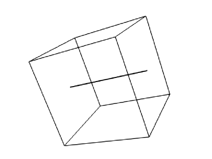
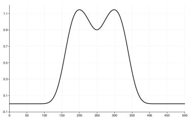
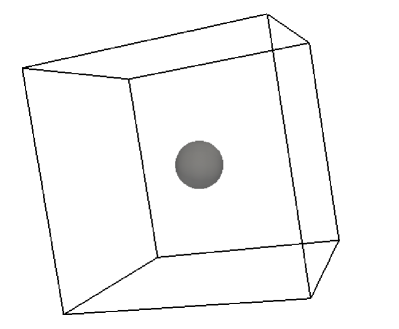
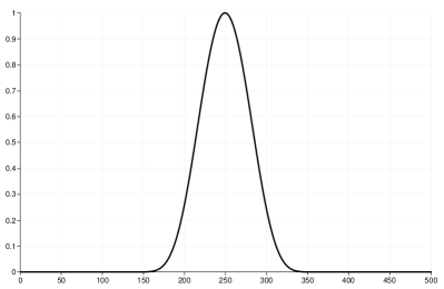
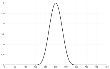
In this section we present several examples for different parameter values of , and for different initial conditions and . Unless otherwise noted in the examples the grid size in space is , resulting in uniform grid spacing . With the Courant–Friedrichs–Lewy (CFL) condition for stability (see, e.g., [24]) has been satisfied for all times and for each of our simulation examples for the Higgs boson equation. For the scaling factor the value has been used. For visualization of the solution we use line plots along either the line segment connecting the midpoints of the computational cube’s faces parallel to the –plane (mid-line parallel to the -axis) or the diagonal line segment connecting the corners and of the unit cube (see Figure 4.1). The horizontal axis shows ranges and respectively on these line plots due to grid the size and due to the diagonal line segment’s length being . For initial conditions we mostly use variations of the compactly supported, infinitely smooth bump function (often used as test functions in the theory of generalized functions (see, e.g., [12]))
| (3.1) |
with center and with radius . Here denotes the euclidean distance between points and . Note that these basic bump functions are nonnegative with maximum value (see Figure 4.2).
Example 1.
In order to examine the convergence properties of our numerical method we look at an example of Equation (2.1) with parameter values , and with the initial conditions.
| (3.2) | ||||
| (3.3) |
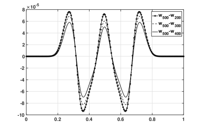
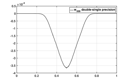
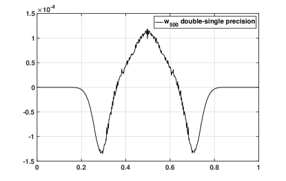
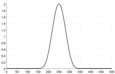
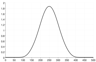
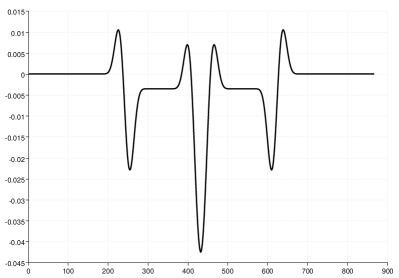
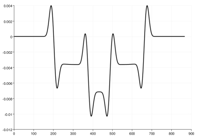
This case will be discussed in more details in Example 6, right now we only look at how solution changes with respect to different grid sizes and different precisions. We vary the grid size in space and compare the results for values , , and to the result with at times and . Since we are working with compactly supported radial solution starting from a bump function, the solution is nonzero only around the center of the computational domain, and we only consider line plots of the pointwise difference instead of , or other global error norms. Figure 4.3 shows stability as the difference between the numerical solutions decreases with increasing values of . The difference is the largest in the regions of high-slope, which moves outward from the center, suggesting that the difference in dispersion plays a role, as suggested for example in [6] for the acoustic wave equation. Figure 4.4 shows the difference between running our code in single and double precision at times and . While the difference is insignificant, and does not seem to increase with time, the double precision code required about more run-time than the single precision code.
Example 2.
As a second computational example we demonstrate that our numerical code can predict the blow up of the sign-preserving solution for not the Higgs boson equation but for the related Klein-Gordon equation with an imaginary mass (see Theorem 1.1 in [27]). For this purpose we set the parameter values as and . As initial conditions we use the bump functions
| (3.4) | ||||
| (3.5) |
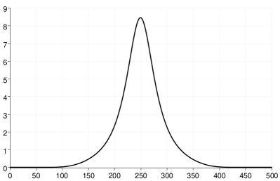
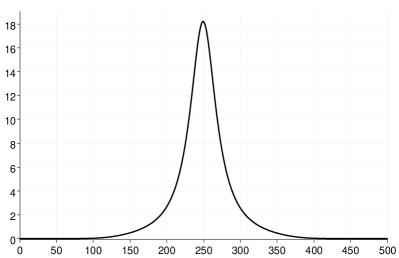
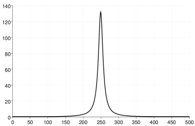
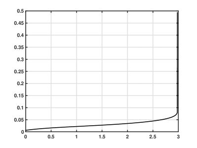
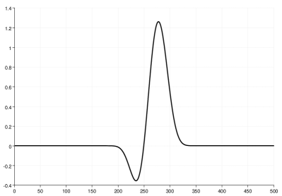
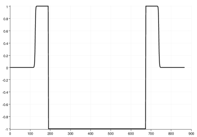
Figure 4.5, parts (a)-(e) show the line plot of the solution for various times. In particularly, we may notice from parts (a) and (b) of Figure 4.5, that from time to time the magnitude of the solution is around and it does not increase, but the compact support of the solution becomes larger instead. After time the magnitude of solution suddenly starts to increase and it reaches the value of approximately by time (part (e) of Figure 4.5). The blow up of the integral shortly after time can be observed on part (f) of Figure 4.5, demonstrating the theoretical results of Theorem 1.1 in [27].
Example 3.
In this example we demonstrate that under certain conditions the solution forms bubbles. For this purpose we reformulate the theoretical results of Corollary 1.4 in [28, page 453]:
Corollary 4.
[28, Corollary 1.4] Bubble forms if the initial data satisfy
| (3.6) | ||||
| (3.7) |
In particular, we consider as initial data the bump functions
| (3.8) | ||||
| (3.9) |
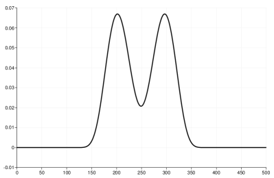
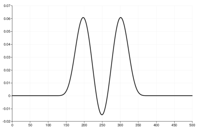
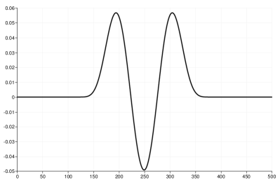
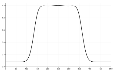
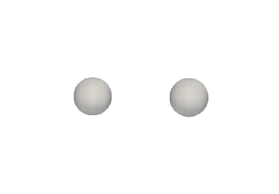
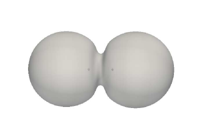
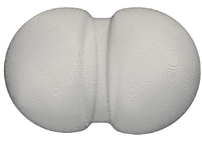
The line plot of the initial function (3.8) is depicted in part (a) of Figure 4.6. Note that the shift makes the initial data and hence the solution radial. The parameter values are , , and hence condition (3.6) is satisfied inside the domain of support. Condition (3.7) is also satisfied for and, by continuity, at least for small . Part (b) of Figure 4.6 shows that at time the values of solution are still all positive inside the domain of support. In parts (c), (d), and (e) of Figure 4.6 at time instances , , and we can see two points, where the solution has zero values with sign change inside the domain of support. These zero places move from the center towards the border of the domain as time goes by. In thee dimensions the isosurface corresponding to these zero values has the shape of a ball (hence the name bubble) centered at the point , as shown in part (f) of Figure 4.6. The radius of the ball increases in time, with the rate of increase decreasing exponentially following the finite speed of propagation .
Example 5.
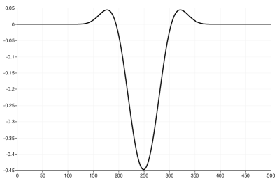
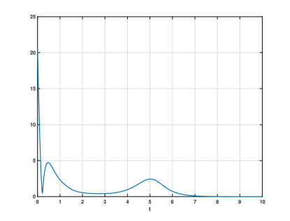
We go back now to Example 3 and continue it for larger time in order to investigate the long-time behavior of the solution. Figure 4.7 shows line plots of the solution for various times. The solution converges to a piecewise constant (step) function with values , , and . The step function’s shape with sharp corners raises the possibility that the solution looses smoothness. In order to examine the question of differentiability we look at how the quantity (related to the second term from equation (2.1)) changes in time. Figure 4.8 shows that the laplacian does not blow up in finite time and hence the solution remains smooth at least up to the second order derivative. Moreover, since converges fast to zero as the time increases, we obtain that equation (2.1) converges to the unforced, damped Duffing equation
| (3.10) | ||||
| (3.11) | ||||
| (3.12) |
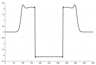
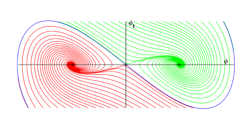
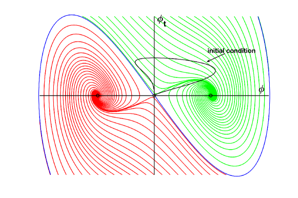
For this ordinary differential equation the two stable equilibrium points are , and the zero is an unstable equilibrium point (see Figure 4.9 for a phase portrait of equation (3.10)). Comparing these values to parts (e)-(f) of Figure 4.7 we can observe that after some initial time during which the dissipative term is not negligible, eventually the solution of the Higgs boson equation (2.1) converges to a step function corresponding to the positive and negative equilibrium points of the Duffing equation (3.10). It is our future plan to investigate and mitigate the numerical difficulty to correctly simulate the places with the sudden changes in the solution. Remarkably, our numerical method did not break down for the time intervals we present here. We will discuss the connection to Duffing equations further in the next examples.
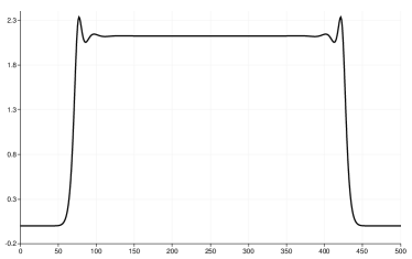
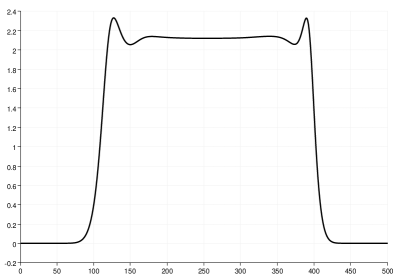
Example 6.
In this example we demonstrate that under some conditions bubbles do not form. This is a new conjecture supported by our computational result, with currently no theoretical proof existing for it in the literature. The parameter values are , as before, and the initial conditions are
| (3.13) | ||||
| (3.14) |
Figure 4.10 shows the line plot of the solution for various times. There are no zeros inside the domain of support, which means that no bubbles formed. Note that this initial data lies on the nonnegative horizontal axis of the phase portrait shown in Figure 4.9, hence, other than the unstable zero equilibrium, this initial data is in the positive equilibrium’s basin of attraction for all in the domain of support. Hence, it should be expected that the solution converges to a step function with values zero and , as suggested by the dynamical properties of the corresponding damped, unforced Duffing equation. The main effect the initially non-negligible dissipative term in equation (2.1) seems to have is to propagate the values in space while they converge to the step function’s values.
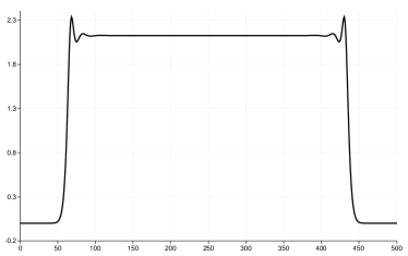
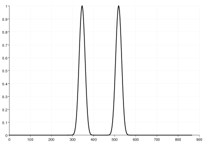
Example 7.
This example shows a slightly more complicated combination of initial conditions in order to demonstrate the connection between the asymptotic behavior of solutions to the Higgs boson equation (2.1) and the associated damped, unforced Duffing equation (3.10). The parameter values are , as before, and the initial conditions are
| (3.15) | ||||
| (3.16) |
Note that in the function of initial condition (3.15) the variable is the first component of the thee-dimensional space variable . Part (b) of Figure 4.11 shows the line plot of the initial function . Part (a) of Figure 4.11 depicts the curve for in the phase portrait of the Duffing equation. Note also that this initial data cannot be made radial by a simple shift in the spatial variable. On the other hand, this initial data lies in the damped, unforced Duffing equation’s stable positive equilibrium’s basin of attraction (and the unstable zero equilibrium point), even though changes sign. Part (a) of Figure 4.11 also suggests that the negative part of the initial function has to be small relative to the positive part of in order for the initial data to stay in the positive equilibrium’s basin of attraction. We can observe on the line plot of solution for time in part (c) of Figure 4.11 that the nonzero part of the solution becomes and stays positive for larger time and indeed it converges to the positive equilibrium point of the damped, unforced Duffing equation, as expected.
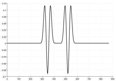
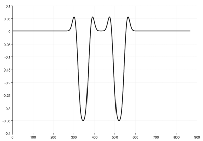
Example 8.
In our final example we look at a more complicated scenario with initial conditions that are the sums of two bump functions:
| (3.17) | ||||
| (3.18) |
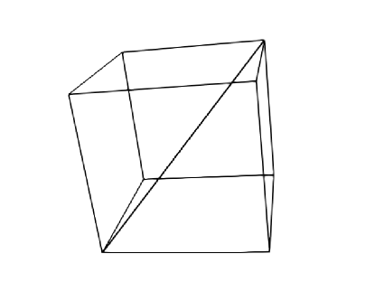
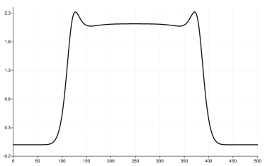
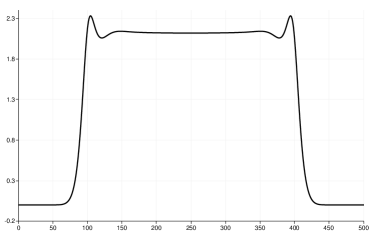
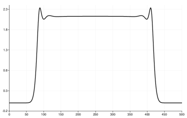
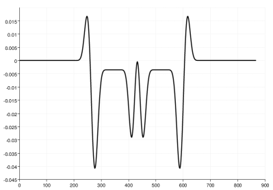
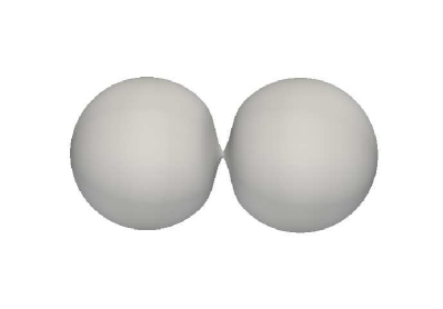
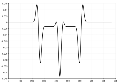
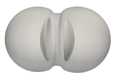
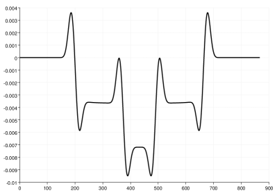
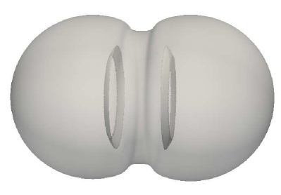
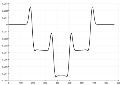
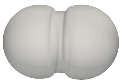
The parameter values are . Figure 4.12 shows a line plot of the first initial data , which cannot be made radial by a simple shift in the spatial variable. Initially the dissipative term is large compared to the speed at which the solution converges to the Duffing equation’s step function. As a result two bubbles form and they interact with each other. For line plots we used the main diagonal line segments of the computational cube, since the centers of the initial conditions’s bump functions are on that diagonal. Figures 4.13-4.15 show the formation and interactions of bubbles. Initially there is no bubble present. After the two bubbles form at around , their size grows continuously in time. Around time the two bubbles touch, and from that time on they are attached to each other. At time (shown on parts (a.1) and (a.2) of Figure 4.14) an additional, tiny bubble forms inside each of the now merged bubbles. These additional bubbles grow (parts (b.1) and (b.2) of Figure 4.14 at time ); then they flatten and become concave (part (c.1) and (c.2) of Figure 4.14 at time ). Later hole forms in these inside bubbles, and they become toroidal (parts (a.1) and (a.2) of Figure 4.15 at time ). Finally they disappear (parts (b.1) and (b.2) of Figure 4.15 at time ). The growth of the larger outer bubble exponentially slows down and it does not seem to change its shape after time . Parts (c.1) and (c.2) of Figure 4.15 show the bubble in a quasi-steady state due to the dissipative term in Equation (2.1) being very close to zero and the solution very close to the step function with constant values and of the corresponding damped, unforced Duffing equation’s equilibrium points.
4 Conclusion
In this paper, we obtained numerical solutions of the Higgs boson equation in the de Sitter spacetime, which is a nonlinear hyperbolic partial differential equation on three spatial dimensions and one time dimension. Our approach was based on a fourth order finite difference method in space and an explicit fourth order Runge-Kutta method in time for the discretization. High performance computations performed using NVIDIA Tesla K40c GPU Accelerator demonstrated existing theoretical results and suggested several previously not known properties of the solution for which theoretical proofs do not exist yet. We conjecture that for smooth initial conditions a smooth solution exists globally for all time; under some initial conditions no bubbles form; and solutions converge to step functions determined by the initial conditions and related to unforced, damped Duffing equations. The theoretical proofs of these conjectures is a future plan along with the numerical treatment of the sharp corners developing in the solutions.
Acknowledgments
The authors acknowledge the Texas Advanced Computing Center (TACC) at The University of Texas at Austin for providing high performance computing and visualization resources that have contributed to the research results reported within this paper. URL: http://www.tacc.utexas.edu. We also gratefully acknowledge the support of NVIDIA Corporation with the donation of the Tesla K40 GPU used for this research.
| (a) Line segment parallel to the -axis | (b) Diagonal line segment | |
|---|---|---|
 |
 |

| Difference between numerical solutions along a line. is the numerical solution for grid size . | |
 |
|
| Numerical solution along a line | |
 |
 |
 |
 |
| (a) Line plot of solution at | (b) Line plot of solution at |
 |
 |
| (c) Line plot of solution at | (d) Line plot of solution at |
 |
 |
| (e) Line plot of solution at | (f) Blow up of around |
 |
 |
| (a) Line plot of solution at | (b) Line plot of solution at |
 |
 |
| (c) Line plot of solution at | (d) Line plot of solution at |
 |
 |
| (e) Line plot of solution at | (f) 3D bubble at |
 |
 |
| (a) Solution along a line at | (b) Solution along a line at |
 |
 |
| (c) Solution along a line at | (d) Solution along a line at |
 |
 |
| (e) Solution along a line at | (f) Solution along a line at |
 |
 |
| (a) Solution along a line at | (b) Solution along a line at |
 |
 |
| (c) Solution along a line at | (d) Solution along a line at |
 |
 |
| (e) Solution along a line at | (f) Solution along a line at |
 |
 |
| (g) Solution along a line at | (h) Solution along a line at |
 |
 |
| (a) Initial function in the phase portrait of the Duffing equation. | |
 |
|
| (b) Line plot of initial function . | (c) Line plot of solution at time . |
 |
 |
 |
| (a.1) Solution along a line at | (a.2) 3D bubbles at |
 |
 |
| (b.1) Solution along a line at | (b.2) 3D bubbles at |
 |
 |
| (c.1) Solution along a line at | (c.2) 3D bubbles at |
 |
 |
| (a.1) Solution along a line at | (a.2) 3D bubbles at |
 |
 |
| (b.1) Solution along a line at | (b.2) 3D bubbles at |
 |
 |
| (c.1) Solution along a line at | (c.2) 3D bubbles at |
 |
 |
| (a.1) Solution along a line at | (a.2) 3D bubbles at |
 |
 |
| (b.1) Solution along a line at | (b.2) 3D bubbles at |
 |
 |
| (c.1) Solution along a line at | (c.2) 3D bubbles at |
 |
 |
References
- [1] Robert A. Adams and John J. F. Fournier, Sobolev spaces, second ed., Pure and Applied Mathematics (Amsterdam), vol. 140, Elsevier/Academic Press, Amsterdam, 2003. MR 2424078
- [2] Utkarsh Ayachit, The ParaView guide: A parallel visualization application, Kitware, Inc., USA, 2015.
- [3] Kartik Chandra Basak, Pratap Chandra Ray, and Rasajit Kumar Bera, Solution of non-linear Klein–Gordon equation with a quadratic non-linear term by adomian decomposition method, Communications in Nonlinear Science and Numerical Simulation 14 (2009), no. 3, 718 – 723.
- [4] A. Bers, R. Fox, C. G. Kuper, and S. G. Lipson, The impossibility of free tachyons, Relativity and Gravitation (C. G. Kuper and Asher Peres, eds.), New York, Gordon and Breach Science Publishers, 1971, pp. 41–46.
- [5] Christophe Bogey and Christophe Bailly, A family of low dispersive and low dissipative explicit schemes for flow and noise computations, Journal of Computational Physics 194 (2004), no. 1, 194 – 214.
- [6] Gary Cohen and Patrick Joly, Construction and analysis of fourth-order finite difference schemes for the acoustic wave equation in nonhomogeneous media, SIAM Journal on Numerical Analysis 33 (1996), no. 4, 1266–1302.
- [7] Sidney Coleman, Aspects of symmetry: Selected Erice lectures, Cambridge University Press, 1985.
- [8] Mehdi Dehghan and Ali Shokri, Numerical solution of the nonlinear Klein–Gordon equation using radial basis functions, Journal of Computational and Applied Mathematics 230 (2009), no. 2, 400 – 410.
- [9] K. Dekker and J.G. Verwer, Stability of Runge-Kutta methods for stiff nonlinear differential equations, Elsevier Science Ltd, North-Holland, Amsterdam, 1984.
- [10] R Donninger and W Schlag, Numerical study of the blowup/global existence dichotomy for the focusing cubic nonlinear Klein–Gordon equation, Nonlinearity 24 (2011), no. 9, 2547.
- [11] Henri Epstein and Ugo Moschella, de Sitter tachyons and related topics, Comm. Math. Phys. 336 (2015), no. 1, 381–430. MR 3322377
- [12] R. Fry and S. McManus, Smooth bump functions and the geometry of banach spaces: A brief survey, Expositiones Mathematicae 20 (2002), no. 2, 143 – 183.
- [13] G. Griffiths and W.E. Schiesser, Traveling wave analysis of partial differential equations: Numerical and analytical methods with Matlab and Maple, Elsevier Science, 2010.
- [14] Lars Hörmander, Lectures on nonlinear hyperbolic differential equations, Mathématiques & Applications (Berlin) [Mathematics & Applications], vol. 26, Springer-Verlag, Berlin, 1997. MR 1466700
- [15] Salvador Jiménez and Luis Vázquez, Analysis of four numerical schemes for a nonlinear Klein–Gordon equation, Applied Mathematics and Computation 35 (1990), no. 1, 61 – 94.
- [16] Doǧan Kaya and Salah M. El-Sayed, A numerical solution of the Klein–Gordon equation and convergence of the decomposition method, Applied Mathematics and Computation 156 (2004), no. 2, 341 – 353.
- [17] H. B. Keller and V. Pereyra, Symbolic generation of finite difference formulas, Math. Comp. 32 (1978), no. 144, 955–971. MR 0494848
- [18] Andrew Liddle, An introduction to modern cosmology, 3 ed., Wiley, 7 2015.
- [19] A. D. Linde, Particle physics and inflationary cosmology, Harwood Academic Publishers, Chur Switzerland New York, 1990.
- [20] J.E. Macías-Díaz and S. Jerez-Galiano, Two finite-difference schemes that preserve the dissipation of energy in a system of modified wave equations, Communications in Nonlinear Science and Numerical Simulation 15 (2010), no. 3, 552 – 563.
- [21] NVIDIA Corporation, CUDA Fortran programming guide and reference, https://www.pgroup.com/doc/pgicudaforug.pdf, 2017.
- [22] , PGI CUDA Fortran compiler, http://www.pgroup.com/resources/cudafortran.htm, 2017.
- [23] J. Rashidinia, M. Ghasemi, and R. Jalilian, Numerical solution of the nonlinear Klein–Gordon equation, Journal of Computational and Applied Mathematics 233 (2010), no. 8, 1866 – 1878.
- [24] Gilbert Strang, Computational science and engineering, Wellesley-Cambridge Press, Wellesley, MA, 2007. MR 2742791
- [25] Inc. The MathWorks, MATLAB and Statistics Toolbox Release 2017b, https://www.mathworks.com/, 2017.
- [26] N. A. Voronov, L. Dyshko, and N. B. Konyukhova, On the stability of a self-similar spherical bubble of a scalar Higgs field in de Sitter space, Physics of Atomic Nuclei 68 (2005), no. 7, 1218–1226.
- [27] Karen Yagdjian, The semilinear Klein-Gordon equation in de Sitter spacetime, Discrete Contin. Dyn. Syst. Ser. S 2 (2009), no. 3, 679–696. MR 2525773
- [28] Karen Yagdjian, On the global solutions of the Higgs boson equation, Communications in Partial Differential Equations 37 (2012), no. 3, 447–478.
- [29] Karen Yagdjian, Global existence of the self-interacting scalar field in the de Sitter universe, arXiv:1706.07703 (2017).
- [30] Muhammet Yazici and Süleyman Şengül, Approximate solutions to the nonlinear Klein-Gordon equation in de Sitter spacetime, Open Physics 14 (2016), no. 1, 314–320.