Dynamics in a one-dimensional ferrogel model: relaxation, pairing, shock-wave propagation

Abstract

Ferrogels are smart soft materials, consisting of a polymeric network and embedded magnetic particles. Novel phenomena, such as the variation of the overall mechanical properties by external magnetic fields, emerge consequently. However, the dynamic behavior of ferrogels remains largely unveiled. In this paper, we consider a one-dimensional chain consisting of magnetic dipoles and elastic springs between them as a simple model for ferrogels. The model is evaluated by corresponding simulations. To probe the dynamics theoretically, we investigate a continuum limit of the energy governing the system and the corresponding equation of motion. We provide general classification scenarios for the dynamics, elucidating the touching/detachment dynamics of the magnetic particles along the chain. In particular, it is verified in certain cases that the long-time relaxation corresponds to solutions of shock-wave propagation, while formations of particle pairs underlie the initial stage of the dynamics. We expect that these results will provide insight into the understanding of the dynamics of more realistic models with randomness in parameters and time-dependent magnetic fields.

I Introduction

Ferrogels, magnetic elastomers, or magnetic gels are smart composite materials Filipcsei et al. (2007) the elastic properties of which are tunable by magnetic fields from outside Ilg (2013); Menzel (2015); Odenbach (2016); Lopez-Lopez et al. (2016). Novel characteristics originate from the composite nature of ferrogels which gives rise to a magneto-mechanical coupling between the embedded magnetic particles and the gel network Frickel et al. (2011); Ilg (2013); Allahyarov et al. (2014). Such a magneto-mechanical coupling can be achieved by constraining the motion of magnetic particles inside pockets of the matrix Frickel et al. (2011); Gundermann and Odenbach (2014); Landers et al. (2015) or by directly anchoring the polymers to the surfaces of magnetic particles Ilg (2013); Frickel et al. (2011); Messing et al. (2011); Roeder et al. (2015). Utilizing this characteristic, a variety of applications such as sensors Szabó et al. (1998); Volkova et al. (2017), actuators Schmauch et al. (2017), tunable devices Deng et al. (2006); Sun et al. (2008), medical scaffolds for tissue engineering Bock et al. (2010); Zhao et al. (2011), and biocomposites for controlled release Müller et al. (2017) have been suggested.

Much effort has also been devoted to the theoretical understanding of the ferrogels. Several routes are suggested and investigated to model these non-trivial materials. At the microscopic scale, bead-spring models to resolve the individual polymer chains connecting the embedded magnetic particles have been studied by means of computer simulations Weeber et al. (2012); Ryzhkov et al. (2015); Weeber et al. (2015a, b). On the macroscale, hydrodynamic theories for ferrogels have been developed Jarkova et al. (2003); Bohlius et al. (2004). Moreover, mesoscopic dipole-spring models Annunziata et al. (2013); Cerdà et al. (2013); Pessot et al. (2014, 2015); Sánchez et al. (2015); Ivaneyko et al. (2015) represent the polymeric matrix by spring-like interactions, while the magnetic particles are resolved and interact with each other via magnetic dipole-dipole interactions. Alternatively, the elastic contributions can be described by matrix-mediated interactions Biller et al. (2014, 2015); Puljiz et al. (2016); Puljiz and Menzel (2017); Menzel (2017) in terms of continuum elasticity theory.

Recently, more attention begins to be paid to dynamic properties. Analogously to the dynamics of magnetic colloidal systems Heinrich et al. (2011); Bloom et al. (2012); Alvarez and Klapp (2013); Dobnikar et al. (2013); Klapp (2016), new configurations or generally novel phenomena observable only in the dynamics are expected to emerge for ferrogels. As an important example, the dynamic moduli/responses of ferrogels have been studied extensively An et al. (2010, 2012); Tarama et al. (2014); Pessot et al. (2016); Nadzharyan et al. (2016); Pessot et al. (2018); Sorokin et al. (2017). To fully describe the dynamics far from equilibrium and the consequent transitions between qualitatively different configurations, it is necessary to address the approach and separation dynamics of magnetic particles under changing mutual magnetic attraction and repulsion. Indeed, the changes in particle distances are well known to affect the material properties of ferrogels. One of the most widely studied phenomena in this regard is the formation of chain-like aggregates which can cause drastic changes in the elastic properties of systems Wood and Camp (2011); Melenev et al. (2011); Zubarev (2013); Romeis et al. (2016); Zubarev et al. (2016a); Lopez-Lopez et al. (2017); Gundermann et al. (2017); Schümann and Odenbach (2017). It has been predicted theoretically that the detachment of magnetic particles in chain-like aggregates can give rise to the pronouncedly nonlinear, so-called superelastic stress-strain behavior Cremer et al. (2015, 2016). The formation of chain-like aggregates has been studied for various dipolar systems, for instance in combination with the Van der Waals interaction van Roij (1996); Kwaadgras et al. (2013).

In a theoretical perspective, the formation of compact chains under magnetic attraction can be viewed as a hardening transition Annunziata et al. (2013), if the particles can come into close contact. Steep changes in elastic properties can be attributed to the hardening due to virtual touching. It is worthwhile to note that the hardening transition implies a double-well structure in the energy. In other words, there exist two different equilibrium configurations, one of which corresponds to the contracted and the other to the elongated systems. Such a configurational bistability, involving the rearrangement of the magnetic particles and the deformation of the gel network, has been widely discussed with different settings Melenev et al. (2011); Annunziata et al. (2013); Biller et al. (2014, 2015); Zubarev et al. (2016b) and therefore seems to be a relatively universal feature. Moreover, one may expect that there exists a regime in between the equilibrium points where configurations become unstable. In short, a type of dynamic mechanism formally similar to spinodal decomposition may play a significant role if attention is extended to dynamics Chaikin and Lubensky (2000).

Spinodal decomposition occurs in various systems, representatively to the phase separation of binary systems described with the aid of the Cahn-Hilliard equation Cahn and Hilliard (1958); Bates and Fife (1993); Elliott and French (1987); Pego (1989). Recently spinodal lines were identified for systems of active Brownian particles Bialké et al. (2013); Speck et al. (2014); Fily et al. (2014); Cates et al. (2010); Stenhammar et al. (2013); Wittkowski et al. (2014). The wetting phenomenon Popescu and Dietrich (2004); Dietrich et al. (2005) also provides an example with a special boundary condition due to the presence of a reservoir. However, there are technical difficulties related to the regularization of the problem Höllig (1983); Barenblatt et al. (1993) which corresponds to the unique characteristics of each system under consideration. In the case of the Cahn-Hilliard equation, for instance, the regularization term contains the free energy cost due to the interface and therefore governs the coarsening dynamics in the long-time scale. Also see, e.g., Refs. Cates et al., 2010 and Wittkowski et al., 2014 for further examples.

In this paper, we study the dynamics of a one-dimensional ferrogel model far from equilibrium. We address questions on the touching and detachment dynamics of magnetic particles. The dipole-spring model is adopted as such a mesoscopic model deals with the configurations of magnetic particles in a direct manner: the magnetic particles are explicitly resolved and the distances between them are simply related to the lengths of springs attached between them. Then a quasi-continuum equation governing the behavior of the system is derived based on a term equivalent to the particle density. Our main results show that the large-scale chain formation dynamics in the long-time regime are governed by shock-wave solutions in the continuum description. With the aid of singular perturbation theory Witelski (1995, 1996) in connection with the Stephan problem Crank (1975); Pego (1989), we can successfully quantify the propagation speed. The origin of our regularization and the relation to general phase separation dynamics are also discussed.

This paper is organized as follows. In Sec. II, a one-dimensional version of the dipole-spring model is introduced. Then we derive a quasi-continuum description of the system and discuss its theoretical properties in Sec. III. Section IV is devoted to illustrate the various observed dynamical scenarios and to develop a “behavioral diagram” for the different types of dynamics, which represents the main result of our study. Lastly, a summary and an outlook are given in Sec. V.

II The model

Our one-dimensional dipole-spring model for a ferrogel system consists of magnetic particles and springs Annunziata et al. (2013); Pessot et al. (2016); Cremer et al. (2017): $N+1$ magnetic particles are connected by $N$ harmonic springs, forming a linear straight chain (see Fig. 1 for a graphical illustration). The number of particles is finite so that the chain has definite boundaries at both ends. In this way, we can perturb the system by applying forces at the boundaries as in the laboratory. The location of the $i$th particle is then represented by $r_{i}$ for $i=1,\ldots,N+1$ and the length of the $i$th spring between the $i$th and the $(i+1)$th particles by $r_{i,i+1}\equiv r_{i+1}-r_{i}$ for $i=1,\ldots,N$. The magnetic dipole moment $\vec{m}_{i}$ is assigned to the $i$th particle, which can be any vector in the three-dimensional space. Below, after switching to a non-zero value, it will be considered as constant in time.

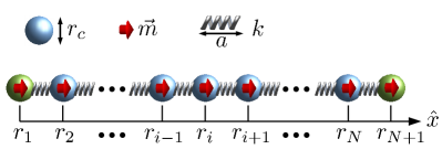
Figure 1: A graphical illustration of our model. Blue and green spheres represent the magnetic particles inside and at the boundaries of the system with the virtual diameter $r_{c}$, respectively, while red arrows correspond to the magnetic dipole moment $\vec{m}$ of the particles. Springs of spring constant $k$ and undeformed length $a$ are depicted as well. In addition, the convention for quantifying the locations of the particles is also illustrated in this figure.

Following previous studies Tarama et al. (2014); Pessot et al. (2016, 2018), we consider the overdamped dynamics of the dipole-spring model as a function of time $t$, governed by equations of motion of the form

$$\Gamma\frac{{\rm d}r_{i}}{{\rm d}t}=-\frac{\partial E_{tot}}{\partial r_{i}}.$$ (1)

Obviously, the form of the total energy $E_{tot}$ determines the dynamical properties of the magnetic chain. In this study, we adopt a simple version of the dipole-spring model in which $E_{tot}$ is given by the sum of elastic interactions, magnetic dipole-dipole interactions, and steric repulsion Pessot et al. (2016); Cremer et al. (2017); Pessot et al. (2018). First, the elastic energy of the harmonic springs takes the form of

$$E_{el}(\{r_{i,i+1}(t)\})=\frac{k}{2}\sum_{i=1}^{N}\left(r_{i,i+1}(t)-a\right)^{2},$$ (2)

where $k$ is the spring constant and $a$ the length of the springs in the undeformed state. Second, the magnetic dipole-dipole interaction energy is given as

$$E_{m}(\{r_{ij}(t)\})=\frac{\mu_{0}}{4\pi} \sum_{j>i}\left[\frac{(\vec{m}_{i}\cdot\vec{m}_{j})}{\left|\vec{r}_{ij}(t)\right|^{3}}\right.$$

$$\left.-\frac{3(\vec{m}_{i}\cdot\vec{r}_{ij}(t))(\vec{m}_{j}\cdot\vec{r}_{ij}(t))}{\left|\vec{r}_{ij}(t)\right|^{5}}\right],$$ (3)

where $\mu_{0}$ is the vacuum permeability, $r_{ij}=r_{j}-r_{i}$, and $\vec{r}_{ij}\equiv r_{ij}\hat{x}$ with the unit vector $\hat{x}$ along the chain axis. For simplicity, we limit ourselves to the case in which the magnetic moments are identical across the whole system, $\vec{m}_{i}\equiv m(\cos{\theta}\,\hat{x}+\sin{\theta}\cos{\phi}\,\hat{y}+\sin{\theta}\sin{\phi}\,\hat{z})$. Then, introducing $b\equiv 1-3\cos^{2}{\theta}$, one can rewrite the magnetic energy in a simpler form

$$E_{m}(\{r_{ij}(t)\})=\frac{\mu_{0}bm^{2}}{4\pi}\sum_{j>i}\frac{1}{\left|r_{ij}(t)\right|^{3}}.$$ (4)

Finally, the steric repulsion preventing a collapse of the system under strong magnetic fields, reads

$$E_{st}(\{r_{i,i+1}(t)\})=\sum_{i=1}^{N}U_{WCA}(r_{i,i+1}(t)),$$ (5)

where $U_{WCA}$ is a modified Weeks-Chandler-Andersen (WCA) type potential in the form Weeks et al. (1971); Pessot et al. (2016)

$$U_{WCA}(r) =\Theta(r_{c}-r)\epsilon^{s}\left[\left(\frac{r}{\sigma^{s}}\right)^{-12}-\left(\frac{r}{\sigma^{s}}\right)^{-6}\right.$$

$$\left.-\left(\frac{r_{c}}{\sigma^{s}}\right)^{-12}+\left(\frac{r_{c}}{\sigma^{s}}\right)^{-6}-\frac{c^{s}(r-r_{c})^{2}}{2}\right],$$ (6)

with the Heaviside step function $\Theta$ and a cutoff distance $r_{c}$. Here, $\sigma_{s}$ and $c_{s}$ are chosen such that $U^{\prime}_{WCA}(r_{c})=0$ and $U^{\prime\prime}_{WCA}(r_{c})=0$ Pessot et al. (2016). The parameter $\epsilon^{s}$ characterizes the strength of the steric repulsion. Now, one can find a set of dynamic equations, substituting the above definitions directly into Eq. (1). Those equations for particles inside as well as at the boundaries of the system are described in detail in Appendix A.

III Formulation of a quasi-continuum theory

To be able to develop a continuum description of the system, we as a major simplification cut the long-range magnetic interaction beyond the nearest-neighbor interaction. We have confirmed from particle-resolved simulations that the overall dynamics with the nearest-neighbor and long-range magnetic interactions are qualitatively equivalent to each other, as far as uniform configurations are adopted as initial conditions (see Sec. III.3).

III.1 Continuum equation

Now the energy is only a function of the distances between adjacent particles as follows:

$$E_{tot}(\{r_{i,i+1}(t)\})=\sum_{i=1}^{N}e\,(r_{i,i+1}(t)),$$ (7)

where $e$ is the pairwise energy given by

$$e(r)=\frac{k}{2}(r-a)^{2}+\frac{\mu_{0}bm^{2}}{4\pi}\frac{1}{r^{3}}+U_{WCA}(r).$$ (8)

The direct analysis of this pairwise energy landscape will help in understanding the equilibrium states as well as the dynamics of the systems and therefore constitutes one of the essential parts of the continuum theory. We address this issue in detail in Sec. III.4.

We then seek a continuum description of the system, introducing a continuous variable $x$, a positional field $r(x,t)$, and its derivatives with respect to $x$, i.e., $r_{x}$, $r_{xx}$, and so on. Following a standard transformation rule $\displaystyle\sum_{i=1}^{N+1}\to\int_{0}^{N}{\rm d}x$, $r_{i+1}-r_{i}\to\partial r/\partial x$, and $\partial/\partial r_{i}\to\delta/\delta r$ (see, e.g., Ref. Doi and Edwards, 1986), we directly obtain from Eq. (1) a fully continuum equation

$$\Gamma r_{t}(x,t)={e}^{(2)}(r_{x}(x,t))r_{xx}(x,t),$$ (9)

where $e^{(i)}(r)\equiv\left(\frac{\partial}{\partial r}\right)^{i}e(r)$ for a general natural number $j$. If the explicit form of the energy is inserted, the continuum equation reads

$$\Gamma r_{t}= kr_{xx}+\frac{3\mu_{0}bm^{2}}{\pi}\frac{r_{xx}}{(r_{x})^{5}}+\epsilon^{s}r_{xx}\Theta(r_{c}-r_{x})$$

$$\times\left[\frac{156}{(\sigma^{s})^{2}}\left(\frac{r_{x}}{\sigma^{s}}\right)^{-14}-\frac{42}{(\sigma^{s})^{2}}\left(\frac{r_{x}}{\sigma^{s}}\right)^{-8}-c^{s}\right].$$ (10)

Two important characteristics of the continuum equation are summarized as follows: First Eq. (9) takes the form of a diffusion equation. However, the diffusion coefficient $e^{(2)}(r_{x}(x,t))$ may have a negative value depending on the value of $m$. Second, the variable $r_{x}$, which determines the sign of $e^{(2)}$, is closely connected to the particle density via the relation $\rho(x,t)=1/r_{x}(x,t)$. Therefore, the particle density controls the dynamics.

III.2 Regularization

We note that, if there exists a range with $e^{(2)}(r_{x})<0$, the continuum equation becomes a type of the forward-backward heat equation which does not necessarily have a unique solution Höllig (1983). It is then mandatory to include an additional term as a regularization, which should be specific for each given physical problem Barenblatt et al. (1993). In our case, the regularization stems from the discrete nature of the system, similarly to the lattice regularization in critical phenomena.

Indeed, the transformation rule $r_{i+1}-r_{i}\to\partial r/\partial x$ involves a truncation of higher order terms $r_{xx}$, $r_{xxx}$, and so on, neglecting corrections from the discreteness of the system. Here, we explicitly take such corrections into account. We consider the differences $\Delta_{i}r\equiv r_{i+1}-r_{i}$ instead of the differential $\partial r/\partial x$ and utilize the functional-derivative technique for discrete variables. As expected, this approach leads to the equations of motion for $i=2,\ldots,N$, described in Appendix A, which formally read

$$\Gamma\frac{{\rm d}r_{i}}{{\rm d}t}=\Delta_{i-1}e^{(1)}(r_{i,i+1}(t)).$$ (11)

Now we probe a continuum description via a transformation from the discrete variable $i=1,2,\ldots,N+1$ to a continuous variable $x$ defined in a domain $0<x<x_{\rm max}$. We choose the midpoint rule to weight equivalently the forces from the right and left sides of the particle under consideration. In other words, a point $i$ in the discrete description corresponds to a range $[x-\Delta x/2,x+\Delta x/2]$ in the continuum description, where $\Delta x$ controls the discreteness of the system. If an asymmetric rule is considered, particles may prefer a motion in a certain direction. Then, with a transformation of the form $x\equiv(i-\frac{1}{2})\Delta x$, the domain on which the newly introduced continuous variable $x$ is defined is determined as $0\leq x\leq x_{\rm max}$ with $x_{\rm max}\equiv(N+1)\Delta x$. Here, we take $x_{\rm max}=1$ by further setting $\Delta x\equiv 1/(N+1)$. In this way, a continuum limit is achieved via $\Delta x\to 0$ or $N\to\infty$. In contrast to that, $r_{xx}$ and higher order derivatives were neglected in the case of the previous transformation rule to the domain $0\leq x\leq N$ with $\Delta x=1$ in Sec. III.1, which was used to derive Eq. (9).

We set up a transformation rule in the form $r_{i}(t)\to r(x,t)/(\Delta x)$, relating the length scale of springs to the corresponding continuous variable $r_{x}$ as $r_{i,i+1}(t)=r_{i+1}(t)-r_{i}(t)\to\frac{r(x+\Delta x,t)-r(x,t)}{\Delta x}=r_{x}(x,t)+\frac{\Delta x}{2}r_{xx}(x,t)+\cdots$. Then we obtain a continuum description from the discrete form in Eq. (9) as follows:

$${\Gamma r_{t}}=(\Delta x) \left\{e^{(1)}\left(\frac{r(x+\Delta x,t)-r(x,t)}{\Delta x}\right)\right.$$

$$\left.-e^{(1)}\left(\frac{r(x,t)-r(x-\Delta x,t)}{\Delta x}\right)\right\}.$$ (12)

Rescaling $x\to x/(\Delta x)$ from the domain $0\leq x\leq 1$ to $0\leq x\leq N+1$, one indeed recovers to leading order the continuum description of the dynamics described by Eq. (9). This can be easily checked by expanding Eq. (III.2) in terms of $\Delta x$ as

$$\Gamma r_{t}= -(\Delta x)\sum_{i=1}^{\infty}\frac{(-1)^{i}}{i!}\left\{\frac{r(x+\Delta x,t)-2r(x,t)+r(x-\Delta x,t)}{\Delta x}\right\}^{i}e^{(i+1)}\left(\frac{r(x+\Delta x,t)-r(x,t)}{\Delta x}\right)$$

$$= -(\Delta x)\sum_{i=1}^{\infty}\frac{(-1)^{i}}{i!}\left\{2\sum_{j=1}^{\infty}\frac{(\Delta x)^{2j-1}}{(2j)!}r^{(2j)}(x,t)\right\}^{i}\left\{\sum_{k=0}^{\infty}\frac{e^{(i+1+k)}\left(r_{x}(x,t)\right)}{k!}\left(\sum_{l=2}^{\infty}\frac{(\Delta x)^{(l-1)}}{l!}r^{(l)}(x,t)\right)^{k}\right\},$$ (13)

where $r^{(i)}\equiv\left(\frac{\partial}{\partial x}\right)^{i}r$. In this way, we maintain aspects of the discrete nature of the system in a quasi-continuum description by letting $\Delta x$ become small but finite. Accordingly, we obtain regularization terms to Eq. (9) from the second- and even higher-order contributions in Eq. (III.2).

Now one could seek for a precise solution, including all terms in Eq. (III.2). Instead, one may truncate them at a certain order, searching for approximate solutions. At this point, we encounter the mathematical issue that different regularization forms may differently alter the dynamics of the forward-backward heat equation Novick-Cohen and Pego (1991); Barenblatt et al. (1993). Rather than rigorously investigating this issue, we here take a pragmatic way using the next-order correction as a feasible form of regularization. This leads to a regularized equation

$$\Gamma r_{t} \approx(\Delta x)^{2}e^{(2)}\left(r_{x}\right)\,r_{xx}+(\Delta x)^{4}\left[\frac{1}{12}e^{(2)}(r_{x})\,r_{xxxx}\right.$$

$$\left.+\frac{1}{6}e^{(3)}(r_{x})\,r_{xx}r_{xxx}+\frac{1}{24}e^{(4)}(r_{x})\,(r_{xx})^{3}\right].$$ (14)

In the end, a certain type of regularization is necessary to evaluate the equations. Our approach has the strong benefit of being fully systematic.

III.3 Initial and boundary conditions

For simplicity, we only consider uniform initial configurations, i.e., $r_{x}(x,t=0)=v^{\rm init}$ with constant $v^{\rm init}$. Boundary conditions in the quasi-continuum theory are carefully determined from the model as follows. First, it is clear that the quasi-continuum equation, e.g., Eq. (III.2), applies to the interior particles. For the boundary particles, additional rules are necessary. Specifically, the boundary particles ($i=1,N+1$) at the left/right ends are governed by

$$\Gamma\frac{{\rm d}r_{1}}{{\rm d}t}=\frac{\partial e(r_{1,2}(t))}{\partial r_{2}},\quad\Gamma\frac{{\rm d}r_{N+1}}{{\rm d}t}=-\frac{\partial e(r_{N,N+1}(t))}{\partial r_{N+1}},$$ (15)

while we have

$$\Gamma\frac{{\rm d}r_{i}}{{\rm d}t}=-\frac{\partial e(r_{i-1,i}(t))}{\partial r_{i}}-\frac{\partial e(r_{i,i+1}(t))}{\partial r_{i}},$$ (16)

for the particles inside the chain. To fill this gap and make the quasi-continuum equations of motion applicable to the boundary particles as well, we introduce hypothetical particles $i=0,N+2$, following the procedure in Ref. Doi and Edwards, 1986. Indeed, Eq. (15) takes the same form as Eq. (16), if the location of the hypothetical particles, $r_{0}$ and $r_{N+2}$, are given by the positions satisfying

$$\frac{\partial e(r_{0,1}(t))}{\partial r_{1}}=0,\quad\frac{\partial e(r_{N+1,N+2}(t))}{\partial r_{N+1}}=0,$$ (17)

so that the forces from the hypothetical to the boundary particles are zero. In the continuum limit, the above relations to lowest order take the form

$$\left.e^{(1)}(r_{x})\right|_{x=\delta\Omega}=0,$$ (18)

where $\delta\Omega=\{0,1\}$.

In practice, the dynamics together with the initial and boundary conditions described above could be interpreted in two different ways as follows: First, one may imagine an infinitely long chain at an unstable fixed point. In this case, the dynamics are initiated by cutting off the outer parts of the chain at the boundaries. Secondly, a stable finite chain with definite boundaries may be considered from the beginning. With $m=0$, for instance, we attain a homogeneous chain as the equilibrium configuration, in which the distances between adjacent particles are equivalent to the equilibrium spring lengths $a$. The dynamics of the system is then initiated by turning on an external magnetic field. This accords with a quenching procedure. In both cases, the interior particles are still in the state of the unstable fixed point directly after the initiation procedures, because the forces from the left and the right particles are well balanced due to the initial homogeneity. This is true as long as only nearest-neighbor magnetic interactions are taken into account. The long-range magnetic interactions slightly affect this picture. However, also in our test simulations including long-range magnetic interactions, we have not observed qualitative differences. As far as the uniform initial configurations are considered, it is always the boundaries from which the dynamics are initiated: for the particles at the left/right boundaries, forces are only acted from the particle on the right/left side at the moment of cutting or quenching.

III.4 Pairwise energy landscape

Mathematically, the pairwise energy $e$ plays a similar role as the free energy does in thermodynamics as thermal fluctuations of the particles Cremer et al. (2017) are neglected in the present study. Above all, (mechanical) equilibrium configurations correspond to the minimum points in the landscape of the pairwise energy, which are determined to lowest order from the condition $e^{(1)}(r_{x})=0$ in the continuum limit. We note that uniform equilibrium configurations automatically satisfy the static equilibrium condition $r_{t}=0$ of our regularized equation, Eq. (III.2). In this study, we are considering a double-well potential, with at least one and at most two locally stable fixed (equilibrium) points: one corresponds to the configuration in which the particles touch each other (high density) while the particles stay away from each other (low density) in the other configuration. Tuning the magnetic moment $m$, one can modulate the number of stable equilibrium points Annunziata et al. (2013). Furthermore, the diffusion coefficient $e^{(2)}(r_{x})$, the sign of which plays a significant role as already discussed in Sec. III.2, is also modulated by the values of $m$. Together with the trivial one for the initial condition, we take into account two independent control parameters, namely, the magnetic moment $m$ and the initial uniform distance between adjacent particle pairs $v^{\rm init}$. Keeping these in mind, we classify the landscapes of the pairwise energy into three categories as shown in Fig. 2.

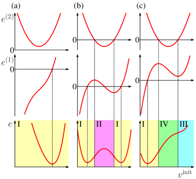
Figure 2: Schematic illustration of the qualitatively different landscapes of the pairwise energies, leading to qualitatively different initial and long-time dynamical behaviors. While regions of $e^{(2)}(v^{\rm init})<0$ in the first row represent spinodal-like intervals, points at $e^{(1)}(v^{\rm init})=0$ in the second row indicate local extrema in the energy density landscapes (see $e$ in the third row). Based on the number of minimum points and the existence of the spinodal-like interval, the landscapes are classified into three qualitative categories, depicted in (a), (b), and (c). Further analyzing the sign of $e^{(2)}$ and the location of the minimum points, we classify the behavior according to the value of $v^{\rm init}$ into different regimes I, II, III, and IV shaded by different colors. See the text for the dynamic scenario corresponding to each regime.

First, we confirm that $e^{(2)}(v^{\rm init})>0$ for all the $v^{\rm init}$ values, if the magnetic moment $m$ is very small [Fig. 2(a)]. In this case, there exists only one minimum in the pairwise energy landscape and the whole range of $v^{\rm init}$ (colored in yellow) belongs to the basin of attraction of the minimum point. From now on, the term Scenario I is used to indicate relaxation dynamics to the stable equilibrium corresponding to this case.

If the magnetic moment is very strong [Fig. 2(c)], once again there is only one stable fixed point which corresponds to a hardened touching configuration of the particles Annunziata et al. (2013). In this case, however, there exists a range with $e^{(2)}(v^{\rm init})<0$ (shaded in green) analogous to the spinodal interval, which divides the range of $v^{\rm init}$ with $e^{(2)}(v_{\rm init})>0$ into two regions: a high-density region (in yellow) forming a basin of the only minimum point and a low-density one (in cyan) separated from the fixed point. Among these three regions, the dynamics around the equilibrium (yellow) is equivalent to Scenario I, while the dynamics starting from the spinodal-like interval (green) and the low-density regime (cyan) are qualitatively different from Scenario I and, respectively, referred to as Scenario III and IV in this paper.

If we consider magnetic moments lower than for the strong-$m$ regime, bistable landscapes appear [Fig. 2(b)]. Once again, separated regions with positive diffusion coefficients (in yellow as before) correspond to Scenario I. In contrast to that, the dynamics starting from the spinodal-like interval in between (shaded in magenta) exhibits a new behavior which is called Scenario II henceforth. Between the bistable [Fig. 2(b)] and very-weak-$m$ regime [Fig. 2(a)], there is an interval with an energy landscape similar to an inversion (e.g., by $v^{\rm init}\to 1/v^{\rm init}$) of the abscissa in Fig. 2(c). As one may expect, no further dynamics qualitatively different from the ones of Scenario I, III, and IV are observed in this case.

IV Scenarios

Using Eq. (III.1), its regularized quasi-continuum version Eq. (III.2), and the analysis of the pairwise energy landscapes in Sec. III.4, we now describe the dynamical scenarios in detail. Even though the quasi-continuum theory is developed using the variable $x$, simulation results are presented in terms of the density as a function of the location of the particles in real space, namely, $\rho_{i}\equiv 1/r_{i,i+1}$ versus $r_{i}$, if not specified otherwise. Similarly, we also use the terms $\rho(x)\equiv 1/r_{x}$, $\rho^{\rm init}\equiv 1/v^{\rm init}$ to lowest order, and so on. Henceforth, time, length, and energies are rendered dimensionless setting $\Gamma/k$, $r_{c}$, and $kr_{c}^{2}$ as units of measurement, respectively. In this unit system, a density of $\rho/\rho_{c}=1$ with $\rho_{c}\equiv 1/r_{c}$ indicates the set of touching adjacent magnetic particles. Moreover, magnetic moments are then measured in a unit of $m_{0}\equiv\sqrt{4\pi kr_{c}^{5}/\mu_{0}}$. In plotting the figures for additional particle-resolved simulation results, values of $a/r_{c}=2.5$, $\epsilon^{s}/(kr_{c}^{2})=1$, and $b=-2$ (assuming that the dipole moments are parallel to the chain axis and all pointing into the same direction) have been used and red cross symbols in the figures represent initial density distributions. Even though only results for $N=100$ are shown, we have observed equivalent dynamics simulating systems with $N=$200, 400, and 800.

IV.1 Scenario I: simple relaxation

We first describe the scenario in the yellow regimes in Fig. 2, in which the uniform initial configuration belongs to the basin of attraction of the equilibrium point given by $e^{(1)}(\rho_{eq})=0$. Moreover, $e^{(2)}(\rho)$ is always positive during the whole time evolution and the regularization is not necessary: direct integration of Eq. (III.1) yields very good agreement with particle-resolved simulations as shown in Fig. 3. The density profiles evolving in time can be either concave ($\rho^{\rm init}>\rho_{eq}$) or convex ($\rho^{\rm init}<\rho_{eq}$).

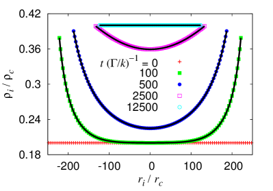
Figure 3: Time evolution of density profile for Scenario I. Density distributions extracted from the particle-resolved simulations are presented by symbols while black lines show the numerical solution of Eq. (III.1). Here, $m=0.1m_{0}$ and $\rho_{i}^{\rm init}=0.2\rho_{c}$. Agreement between particle simulation and numerical solution of the theory is manifested clearly. These results are also depicted in more detail in MOVIE I of ESI sup .

IV.2 Scenario II: pair formation

Now, we consider the dynamics in the bistable regime with initial configurations in the spinodal-like interval, i.e., the range satisfying $e^{(2)}(\rho^{\rm init})<0$. As depicted by black lines in Fig. 4, there are two different states of energetic minima, in both of which the corresponding configurations are uniform. In the particle-resolved simulations, we observe formations of particle pairs. As represented by high-density points in Fig. 4, the pairs consist of two touching particles, appearing in a row along the chain. Both of the two densities computed from the pairs as well as from the stretched springs between the pairs coincide with the density values of the minimum points in the pairwise energy. This indicates that the heterogeneous configurations are stable in the discrete systems in the absence of fluctuations. Therefore, in the particle-resolved simulations, the relaxation to the global minimum state with a uniform configuration is not observed. In addition, we note that, near the spinodal lines of $e^{(2)}=0$, clusters with a number of touching particles larger than 2 (high-density spinodal line) or stretched springs with only one magnetic particle in between (low-density spinodal line) are observed as stable configurations in the simulations.

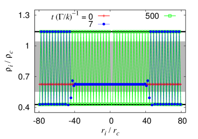
Figure 4: Density distributions in Scenario II. Symbols display the simulation results and thick black lines represent the uniform configurations corresponding to the local minimum points of the pairwise energy. The region shaded in gray represents the spinodal-like interval. In this figure, $m=0.9m_{0}$ and $\rho_{i}^{\rm init}=0.625\rho_{c}$. For more details, see MOVIE II of ESI sup .

We then turn to the continuum theory. For this scenario, a regularization is mandatory. There are two different candidates for the boundary condition, both of which satisfy Eq. (18), as we consider the bistable regime. Here, let us take the global minimum state as a boundary condition. Then it is observed that numerical solutions of the continuum equation (see Appendix C for further details) converge to the global minimum state with a uniform configuration in contrast to the particle-resolved simulations. Such a disagreement may imply a failure of the continuum theory in providing a full description in this regime. Indeed, it is well known from the $\Gamma$-convergence theory that the solutions to the Cahn-Hilliard equation asymptotically approach to the global minimum point Modica (1987); Pego (1989); Braides (2002). Similarly, we conjecture that the asymptotic solutions to our quasi-continuum theory are given as the uniform configuration at the global minimum point. This may, for instance, be due to our non-exact regularization terms in the quasi-continuum description together with the numerical scheme adopted in the integration of the continuum equation that includes additional diffusion. Thus, the bistability is at present only visible in our discrete particle simulations.

For further insight, we inspect the individual particle dynamics. Let us consider a particle and its two nearest neighbors as well as the two springs connecting them. With the two distances between the two particle pairs, $r_{1}$ and $r_{2}$, the corresponding energy can be written as $E_{in}(r_{1},r_{2})=e(r_{1})+e(r_{2})$. Then introducing new variables $L\equiv r_{1}+r_{2}$ and $l=r_{1}-r_{2}$, we first confirm that the state of $l=0$ with a homogeneous configuration corresponds to a fixed point of the dynamics because

$$\left.\frac{\partial E_{in}}{\partial l}\right|_{l=0}=\left[\frac{1}{2}e^{(1)}\left(\frac{L+l}{2}\right)-\frac{1}{2}e^{(1)}\left(\frac{L-l}{2}\right)\right]_{l=0}=0.$$ (19)

Meanwhile, the fixed point of $l=0$ is unstable if $e^{(2)}(L/2)=e^{(2)}(r_{1})=e^{(2)}(r_{2})<0$ as one can easily verify from the corresponding Hessian matrix

$$\left({\begin{array}[]{cc}\frac{1}{2}e^{(2)}(L/2)&0\\ 0&\frac{1}{2}e^{(2)}(L/2)\\ \end{array}}\right).$$ (22)

For $e^{(2)}(L/2)<0$, as in this case, it is straightforward to describe the onset of the scenario: dynamics initiated from the boundary (as already discussed in Sec. III.3) penetrates into the inner part of the chain, perturbing particles in the local maximum state. Then one may expect a heterogeneity in the configuration (i.e., $l\neq 0$) as a consequence of the above spinodal-like decomposition mechanism, which underlies the formation of touching particle pairs. As shown in Fig. 4, densities for touching pairs and for the stretched springs between pairs agree well with the values of the two local minimum points. Consequently, the resulting configuration remains stable once the localized spinodal-like decomposition dynamics are accomplished.

IV.3 Scenario III: shock-wave propagation

In this scenario, the most important feature observed in the particle-resolved simulations is the generation of sharp interfaces which divide the chain into macroscopic high-density clusters and stretched low-density configurations, as shown in Fig. 5. Specifically, we observe movements of the interfaces between these regions, which are initially formed at the ends of the chain. Such movements or propagations of the interfaces, for instance, in the regime of strong magnetic fields [cyan in Fig. 2(c)], make the high-density clusters of touching particles grow towards the center of the chain. As one can see, the widths of interfaces are of the order of the distance between adjacent particles. Before we proceed, we note that, in this section as well as in Sec. IV.4 devoted to Scenario IV, only the touching dynamics are analyzed. The extension of the discussion to the detaching dynamics corresponding to the case between very weak or vanishing $m$ and the intermediate bistable regime would be straightforward.

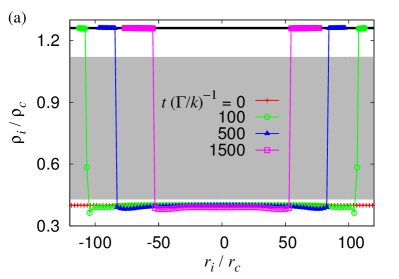
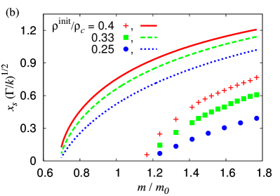
Figure 5: Results for Scenario III of shock-wave propagation. (a) Density distributions for $m=1.7m_{0}$ and $\rho_{i}^{\rm init}=0.4\rho_{c}$ are shown, indicating high-density clusters at the ends and a low-density region on the inside. Symbols represent the particle-resolved simulation results while the equilibrium density computed from the theory is represented by a black line. Sharp interfaces between high- and low-density clusters are manifested clearly. A movie (MOVIE III) describing the time evolution can be found in ESI sup . (b) Values of the coefficient $x_{s}$, obtained from the particle-resolved simulations (symbols) and the singular perturbation theory (lines), are compared to each other.

According to the analysis on the level of individual particles, the dynamics are initiated from the boundary as before. In contrast to Scenario II, however, the perturbation from the boundary does not affect the particles inside immediately as they roughly remain in a locally stable state. If the effects from the boundaries are not too strong (this corresponds to Scenario I, in which the initial state already belongs to the basin of the equilibrium point), then the relation $e^{(2)}(L/2)>0$ can still be satisfied, keeping the configuration somewhat uniform. As a consequence, in Scenario I particles persistently move towards the center during the whole dynamics.

As a new feature, in Scenario III, the distortion at the boundaries is strong enough due to such a large difference between the initial and equilibrium densities that the stability of the uniform configuration can be disturbed. In this case, the $l=0$ (homogeneous) configuration becomes unstable for particles at interfaces. With this mechanism, the particles at interfaces can move into the direction opposite to the motion of most other particles in this half of the chain as well as of the interface, resulting in touching to the high-density cluster at the corresponding end of the chain. Subsequently, a sharp undershoot is developed in the density distribution at the interfaces.

In terms of the continuum theory, this scenario corresponds to shock-wave propagations Witelski (1995). With a specific regularization, we are able to describe the shock with the aid of singular perturbation theory. Here, we briefly summarize the procedure (see Appendix B for the details). According to singular perturbation theory, the structure of the shock is quantified by the values of $r_{x}$ behind and in front of the discontinuity or $v_{-}$ and $v_{+}$ as defined in Appendix B, which should satisfy $e^{(1)}(v_{-})=e^{(1)}(v_{+})$. Among the candidates satisfying the condition, certain values of $e^{(1)}(v_{\pm})$ are selected, depending on the specific form of regularization. For the regularization in Eq. (III.2), we find that the shock wave satisfies the equal area rule Pego (1989) or equivalently the common tangent construction (see, e.g., Refs. Witelski, 1996 and Wittkowski et al., 2014 for other types of solution). From the determined values of $v_{\pm}$, we can then compute the similarity coefficient $x_{s}$ which means the factor in a similarity relation of the type $N_{T}=x_{s}\sqrt{t}$, where $N_{T}$ is the number of the particles in the high-density cluster. As this coefficient determines how fast the shock-wave propagates, it is of interest to probe quantitatively its values which are presented in Fig. 5 (b). As one can see, the overall behavior is described qualitatively by the theory, but with non-negligible errors. Regarding the fact that here we consider the dynamics near a singularity, this type of error seems to be acceptable.

In addition to that, we can further classify the density profiles of this scenario into two cases: The first one corresponds to the case of $\rho^{\rm init}<\rho_{+}\equiv 1/v_{+}$ to lowest order. As the outer layer solution should connect the initial condition $v^{\rm init}$ and $v_{+}$, the existence of an undershoot in the density profile at the shock is expected. Considering the conservation of particles involved in determining the shock structure Crank (1975); Pego (1989); Witelski (1995), we speculate that a mechanism similar to the generation of depletion regions in solidification processes ahead of the solidification front Sandomirski et al. (2011) seems to play a role in this undershoot generation. If the initial density is high enough, such an undershoot disappears and the solution becomes monotonic. In particle-resolved simulations, one may take the concavity/convexity of the interior part of chains as an index to identify the existence of the undershoot in density profiles.

IV.4 Scenario IV: shock wave of pairs

Lastly, we describe Scenario IV. In this scenario, the initial configurations reside in the spinodal-like interval as $e^{(2)}(v^{\rm init})<0$. Therefore, as in Scenario II, complicated configurations consisting of touching particle pairs develop from the beginning of the dynamics. In contrast to Scenario II, however, the density extracted from the stretched springs does neither correspond to the stable solution nor does it belong to the basin of the stable fixed point. Moreover, the stretched configurations are no longer in the spinodal-like interval, once the spinodal-like dynamics are settled. Therefore, one may expect a shock-wave dynamics as in Scenario III. Indeed, we observe once again a shock-wave propagation, see Fig. 6. In this scenario, it is the touching of the touching pairs instead of the single particles which constitutes the dynamics of the shock wave. We also confirm that the numerical integration of the theory exhibits similar time evolution in the density distributions as shown in Appendix C. However, a quantitative description of the shock structure/position in terms of the theory is still in progress.

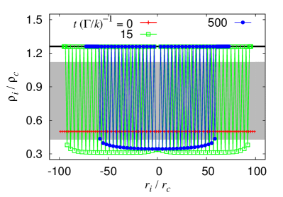
Figure 6: Density profiles for Scenario IV. As before, symbols, black line, and gray region indicate the particle-resolved simulation results, the equilibrium density predicted by the theory, and the spinodal-like interval, respectively. Here, $\rho_{i}^{\rm init}=0.5\rho_{c}$ and $m=1.7m_{0}$. The pair formation as well as the shock-wave propagation are observed clearly. For more details, see MOVIE IV of ESI sup .

IV.5 Dynamical state diagram

Putting together the four different scenarios, we present in Fig. 7 a dynamical state diagram of the one-dimensional dipole-spring model. No other qualitatively different scenario was found for the present energy with at most two equilibrium points. Schematic figures represent the density profiles at intermediate time scales after the settlement of the initial pair-formation dynamics but before full equilibration. Here, let us elucidate the observed phenomena.

When the magnetic moment is very small ($m/m_{0}\lesssim 0.21$), the effects of the magnetic interactions are negligible and the touching/detachment dynamics does not play a significant role. If we consider the regime of strong magnetic moments ($m/m_{0}\gtrsim 1.15$), the magnetic interactions significantly affect the overall dynamics. As the magnetic interactions are strong, it is the touching of particles separated in the low initial density regimes (cyan) that triggers the shock-wave dynamics. Here, we further note that, phenomenologically, the contraction of the chain is mainly governed by this shock-wave dynamics.

In the case of the spinodal-like mechanism (green and magenta), the pair formation rather contributes to the redistribution of particles and sometimes even causes an increase of the chain length. Here, the dissipation of energy is faster during the initial stage of the pair formation than during the shock-wave propagation. This seems plausible as the instabilities are localized only in the vicinity of the interfaces in the case of the shock-wave propagation dynamics, while they are distributed across the whole system in the spinodal-like case, simultaneously contributing to the energy dissipation during the pair formation.

Opposite phenomena are observed in the range of $0.21\lesssim m/m_{0}\lesssim 0.40$. Even though the magnetic interactions play a significant role in this regime, what we observe is mostly the separation of particles as the magnetic interactions are still weak in this case. Specifically, we observe separation of magnetic particles starting from the boundaries and propagations of sharp interfaces extending expanded regions of the chain from the left/right ends to the center in the high-density regime (cyan). Similarly, in the intermediate-density regime (green), the separation of particles that form pairs due to the spinodal-like mechanism in the initial stage of the dynamics underlies the shock-wave propagation.

In the intermediate $m$-regime, at $0.48\lesssim m/m_{0}\lesssim 1.15$ (magenta), we observe heterogeneous configurations as resulting equilibrium states due to the bistability of the energy. However, if the dynamical theory based on the quasi-continuum equation of motion Eq. (III.2) is evaluated, we are not able to describe the emergence of this Scenario II. Only the relaxation dynamics to the global minimum states are found.

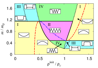
Figure 7: Dynamical state diagram. Black dotted lines indicate boundaries between dynamical scenarios, while black solid lines discriminate between the states with different equilibrium configurations, see Fig. 2. Red dashed lines represent the equilibrium states of global energetic minima while the blue dotted-dashed line corresponds to the unstable local maximum points in the pairwise energy. We note that the black solid lines between yellow and magenta areas and the black dotted lines between green and cyan regimes and between green and yellow areas constitute the spinodal line with $e^{(2)}(\rho)=0$. Additional black dotted lines inside cyan regions are of $\rho_{+}/\rho_{c}$ for $m/m_{0}\gtrsim 1.15$ and of $\rho_{-}/\rho_{c}$ for $0.21\lesssim m/m_{0}\lesssim 0.48$. We also note that green and magenta regions are the spinodal-like intervals while yellow regions correspond to the basins of attraction of the equilibrium points. The same colors as in Fig. 2 are used to identify the different dynamical scenarios. Schematic density profiles of corresponding dynamical scenarios are indicated.

IV.6 General discussion

Lastly, we qualitatively discuss our results in comparison to general aspects of the dynamics of phase separation. First, in the present case, it is found that the boundaries initiate the dynamics of the systems, instead of thermal fluctuations as for general scenarios of phase separation. Secondly, the growth mechanism of touching clusters (or their separation dynamics) following the spinodal-like initial dynamics is different from the phase separation due to different conservation laws. In sharp contrast to scenarios of typical phase separation, in our case the overall size of the system may change over time. Thus the particle number is conserved in the dipole-spring system, instead of the global density as in typical scenarios of phase separation. This counteracts the coexistence of two phases of different densities but rather promotes the transition to only one phase. Consequently, the shock-wave propagation dominates the long-time relaxation dynamics of the system, driving the change in extension of the chain and promoting the overall transformation of the whole system.

Apart from that, as a technical detail, the underlying background of the regularization is also different in our quasi-continuum description. While, for instance, the interface itself contributes to the free energy in the Cahn-Hilliard equation in the form of gradient terms Cahn and Hilliard (1958); Pego (1989), it is only the discreteness of the system that gives rise to the regularization in our case. We stress, however, that the spinodal-type mechanism based on the structure of the underlying energy is formally rather analogous, leading to the emergence of pair/cluster formation.

Altogether, the touching/detachment dynamics can be related to a spinodal-type mechanism, while the interfacial shock-wave propagation governing the long-time dynamics in certain cases may rather be comparable to a scenario of domain growth. Different scenarios of touching/detachment dynamics are summarized in Table 1.

Scenario	$\rho_{i}(r_{i})$	Intermediate configuration	Equilibrium state
II			Heterogeneous
III			Uniform, $\rho>\rho_{c}$
			Uniform, $\rho<\rho_{c}$
IV			Uniform, $\rho>\rho_{c}$
			Uniform, $\rho<\rho_{c}$

Table 1: Schematic graphical representations of the scenarios involving the touching/detachment dynamics. While schematic figures for the intermediate density profiles are displayed in the second column, corresponding intermediate configurations during the relaxation to stationary equilibrium states are briefly portrayed in the third column. Values of $m$ and $\rho^{\rm init}$ can be identified from the dynamical state diagram in Fig. 7 by comparing the corresponding schematic plots in the second column. In the last column, the characteristics of their final stationary equilibrium configurations are summarized. In all of the three scenarios, a spinodal-type mechanism underlies the initial touching and detachment dynamics of the magnetic particles. However, the long-time dynamics are always dominated by the shock-wave propagation, except for Scenario II, in which there is no further long-time relaxation dynamics.

V Summary and outlook

Until now, we have investigated the relaxation dynamics of a one-dimensional dipole-spring model. We have revealed that a type of spinodal decomposition mechanism plays a central role in the touching or detachment dynamics of magnetic particles and that shock-wave-type propagations can dominate the long-time relaxation dynamics to the equilibrium states. The boundary effects are shown to be an essential ingredient for the initiation and the subsequent qualitative appearance of the dynamics, while the discreteness of the system regularizes the continuum equation of motion. It is remarkable that even these simple one-dimensional systems exhibit heterogeneous scenarios in spite of the homogeneity in initial and, mostly, equilibrium configurations. A variety of rich dynamics involves the interplay between the formation of particle pairs and the shock-wave propagation.

There still remains plenty of space for further extensions of the present study. First of all, the response of the system to time-dependent magnetic fields is of interest. Specifically, effects of the touching/detaching dynamics on the dynamic moduli of the system Pessot et al. (2016, 2018) may deepen the understanding of the magneto-mechanical couplings in ferrogels. Extensions of the model to two- and three-dimensional systems are also an important step. In part, we anticipate similar dynamics for strong directed magnetic interactions, as then, likewise, one-dimensional chain-like aggregations will form aligned along the direction of an applied external magnetic field Pessot et al. (2016); Gundermann et al. (2017); Schümann and Odenbach (2017); Pessot et al. (2018). Already, our one-dimensional simulation results suggest that the global minimum states in the intermediate regime could be non-uniform. Even more possibilities arise in two or three dimensions and, therefore, even richer dynamics are expected to be observed. In addition to that, effects of thermal fluctuations should be clarified as well Cremer et al. (2017). For example, if heterogeneous initial configurations are taken into account, we observe the onset of the shock-wave propagation in the particle-resolved simulation for long-range magnetic interactions even from the interior of the chain. One may expect similar phenomena in the system induced by thermal fluctuations, which may correspond to the nucleation of dense clusters or soft components.

We expect that the results discussed in this study can be confirmed from experiments. Indeed, the experimental technology these days enables researchers to capture the configuration at a certain time point Gundermann et al. (2017) or to provide a temporal resolution of the dynamics of corresponding systems Puljiz et al. (2016); Huang et al. (2016). Therefore, supported by quantitative analysis of the data, the formation of particle pairs and the propagation of sharp interfaces might be verified. Still, there is a possibility that the imperfections inherent in experimental samples may obscure such verification. However, there are efforts to construct uniform nanocomposite samples Feld et al. (2017). With the aid of such an approach, the rigorous comparison between theory and experiments could be achieved.

Meanwhile, especially in interpreting possible experimental results, randomness in the network connectivity as well as in the arrangement and size of the magnetic particles should be taken into account. Still, one may expect a similar dynamics, consisting of pair formation and shock-wave propagation. For example, touching pairs and compact chain formation are observed even in three-dimensional inhomogeneous dipole-spring systems based on experimentally observed particle configurations Pessot et al. (2018). However, details such as the size of the touching clusters or the initiation mechanism of exit the dynamics may differ. If heterogeneity is introduced in the spring constant, softer parts of the chain may form a touching cluster more easily than other parts of the system and, therefore, the chain formation dynamics could be initiated in various parts of the system. In this case, we speculate that a kind of coupling between the interfaces may play a certain role. Verification of such couplings could be a challenging task in theoretical as well as in experimental studies.

In short, we expect that our results may serve as an essential building block in understanding the dynamics of more realistic models for ferrogels. However, we also note that a further adjusted continuum theory with fine-tuned regularization terms should be devised to fully describe the whole dynamics, especially in the bistable regime. This is left for future works.

Appendix A Equations of motion for the particles

We describe the equations of motion for the particles in the magnetic chain in detail. The equations for the boundary particles are shown explicitly as well.

Obviously, the term on the right-hand side of Eq. (1) consists of three parts. The first one of them, resulting from the elastic energy, reads

$$-\frac{\partial E_{el}}{\partial r_{i}} =k(r_{i+1}-r_{i})-k(r_{i}-r_{i-1})$$ (23)

for $i=2,\ldots,N$ and

$$-\frac{\partial E_{el}}{\partial r_{1}}=k(r_{2}-r_{1}-a),\quad-\frac{\partial E_{el}}{\partial r_{N+1}}=-k(r_{N+1}-r_{N}-a).$$ (24)

Second, the contributions from the magnetic dipole-dipole interaction take the form

$$-\frac{\partial E_{m}}{\partial r_{i}} =\frac{3\mu_{0}bm^{2}}{4\pi}\left[-\sum_{j>i}\frac{1}{\left(r_{j}-r_{i}\right)^{4}}+\sum_{j<i}\frac{1}{\left(r_{j}-r_{i}\right)^{4}}\right]$$ (25)

for $i=2,\ldots,N$, and

$$-\frac{\partial E_{m}}{\partial r_{1}}=-\frac{3\mu_{0}bm^{2}}{4\pi}\sum_{j=2}^{N+1}\frac{1}{\left(r_{j}-r_{1}\right)^{4}},\quad-\frac{\partial E_{m}}{\partial r_{N+1}}=\frac{3\mu_{0}bm^{2}}{4\pi}\sum_{j=1}^{N}\frac{1}{\left(r_{j}-r_{N+1}\right)^{4}}.$$ (26)

We note that the nearest-neighbor magnetic dipole-dipole interaction is obtained from the above equations by constraining the summations in $j$ to nearest neighbors.

Lastly, we have

$$-\frac{\partial E_{st}}{\partial r_{i}} ={f}_{st}(r_{i,i+1})-{f}_{st}(r_{i-1,i})$$ (27)

for $i=2,\ldots,N$ and

$$-\frac{\partial E_{st}}{\partial r_{1}} ={f}_{st}(r_{1,2}),\quad-\frac{\partial E_{st}}{\partial r_{N+1}}=-{f}_{st}(r_{N,N+1})$$ (28)

from the steric repulsion energy, where

$$f_{st}(r) \equiv\epsilon^{s}\Theta(r-r_{c})\left[-\frac{12}{\sigma^{s}}\left(\frac{r}{\sigma^{s}}\right)^{-13}+\frac{6}{\sigma^{s}}\left(\frac{r}{\sigma^{s}}\right)^{-7}-{c^{s}(r-r_{c})}\right].$$ (29)

Appendix B Singular perturbation theory

We define $v\equiv r_{x}$ and rescale the time variable by introducing $\tau\equiv(\Delta x)^{2}\,t$ for convenience. Then Eq. (III.2) reads

$$\Gamma v_{\tau}=\left[e^{(1)}(v)+(\Delta x)^{2}\left(\frac{1}{12}e^{(2)}(v)\,v_{xx}+\frac{1}{24}e^{(3)}(v)\,(v_{x})^{2}\right)\right]_{xx}.$$ (30)

Introducing the extended variable $\displaystyle\tilde{x}=\frac{x-s(\tau)}{(\Delta x)}$, we probe an interlayer solution which describes the behavior of the system in the vicinity of the shock front at $s(\tau)$. Under a change of variables $v=\tilde{v}(\tilde{x},\tau)$ with $\displaystyle v_{x}=\frac{1}{\Delta x}\tilde{v}_{\tilde{x}}$ and $\displaystyle v_{\tau}=\tilde{v}_{\tau}-\frac{\dot{s}(\tau)}{\Delta x}\tilde{v}_{\tilde{x}}$, Eq. (30), to the leading order of $\Delta x$, becomes

$$\left(e^{(1)}(\tilde{v})+\frac{1}{12}e^{(2)}(\tilde{v})\,\tilde{v}_{\tilde{x}\tilde{x}}+\frac{1}{24}e^{(3)}(\tilde{v})\,(\tilde{v}_{\tilde{x}})^{2}\right)_{\tilde{x}\tilde{x}}=0,$$ (31)

which has a solution of the form

$$e^{(1)}(\tilde{v})+\frac{1}{12}e^{(2)}(\tilde{v})\,\tilde{v}_{\tilde{x}\tilde{x}}+\frac{1}{24}e^{(3)}(\tilde{v})\,(\tilde{v}_{\tilde{x}})^{2}=A\tilde{x}+B.$$ (32)

For the interlayer solutions $\tilde{v}$ and $\tilde{v}_{\tilde{x}}$ must approach constant values $v_{\pm}$ and $0$ as $\tilde{x}\to\pm\infty$ and, therefore,

$$A=0,\quad B=e^{(1)}(v_{-})=e^{(1)}(v_{+}).$$ (33)

Further multiplying by $\tilde{v}_{\tilde{x}}$, we also find

$$\left(B\tilde{v}\right)_{\tilde{x}}=\left(e(\tilde{v})+\frac{1}{24}e^{(2)}(\tilde{v})\,(\tilde{v}_{\tilde{x}})^{2}\right)_{\tilde{x}},$$ (34)

which leads to the equal-area rule Pego (1989); Witelski (1996) for the interlayer solution of the form

$$B(v_{+}-v_{-})=e(v_{+})-e(v_{-}).$$ (35)

Numerically solving Eqs. (33) and (35), one can compute the values of $v_{+}$ and $v_{-}$, which specify the structure of the shocks. The construction of the equal area rule and the resultant shock structures are presented in Figs. 8(a) and (b).

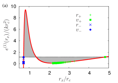
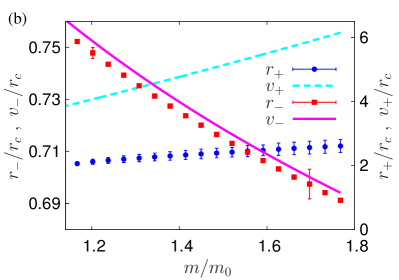
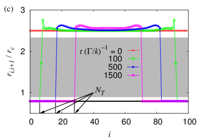
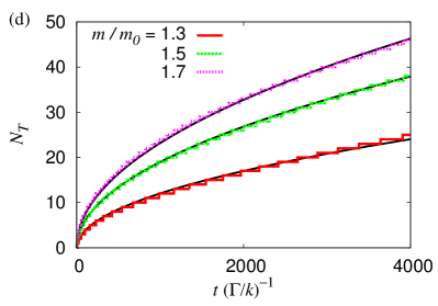
Figure 8: (a) How the equal area rule applies in practice is described: the structures of the shocks are given by the filled blue circle ($v_{-}$) and the filled green square ($v_{+}$), corresponding to the intersection points between the red line representing $e^{(1)}$ and the black dotted line, where $v_{-}$ and $v_{+}$ are the values of $r_{x}$ behind and in front of the shock. The gray areas above and below the black dotted line need to be equal to each other. Plus and cross symbols representing the particle-resolved simulation results are displayed as well. Specifically, $r_{-}$ and $r_{+}$ are given as the lengths of the springs in front of and behind the abrupt jump in the density, respectively. (b) The values of $v_{+}$ and $v_{-}$ (magenta and cyan solid lines) computed from Eqs. (33) and (35) are compared with the particle-resolved simulation results, $r_{+}$ and $r_{-}$ (blue circles and red squares). We note that the values on the left axis correspond to those of $r_{-}$ (red squares) and $v_{-}$ (magenta solid line), while $r_{+}$ (blue circles) and $v_{+}$ (cyan dashed line) are represented by the axis on the right. (c) Fig. 5(a) for Scenario III is replotted in terms of $r_{i,i+1}$ as a function of $i$. The values of $N_{T}$ are explicitly depicted by arrows. (d) The values of $N_{T}$ as functions of time $t$ are plotted for $m=1.3m_{0}$, $1.5m_{0}$, and $1.7m_{0}$ with $\rho_{i}^{\rm init}=0.4\rho_{c}$. We extract the values of $x_{s}$ by numerically fitting the results to the relation $N_{T}=x_{s}\sqrt{t}$ (black solid lines), which here are found to be $x_{s}(\Gamma/k)^{1/2}=$ 0.380 ($m/m_{0}=1.3$), 0.600 ($m/m_{0}=1.5$), and 0.732 ($m/m_{0}=1.7$).

We turn to the propagation speed of the shock-wave front $s(\tau)$. As our equation of motion in the leading order takes the form of a diffusion equation, we consider a similarity solution $U(z)=v(x,\tau)$ with the similarity variable $z\equiv x/\sqrt{\tau}$. The equation of motion in the leading order follows as

$$\Gamma v_{\tau}=(e^{(2)}(v)\,v_{x})_{x}$$ (36)

in terms of $x$ and $\tau$. It can be rewritten as

$$\frac{\Gamma}{2}z\frac{{\rm d}U(z)}{{\rm d}z}=-\frac{{\rm d}}{{\rm d}z}\left(e^{(2)}(U)\frac{{\rm d}U(z)}{{\rm d}z}\right)$$ (37)

in terms of the similarity variable $z$. In particular, the quantity of interest is the coefficient $x_{s}$ which is defined by a similarity relation $s(\tau)=x_{s}\sqrt{\tau}$. Quantifying the values of $x_{s}$ with the Whitham’s derivation Whitham (1999), one can describe the dynamics of the shock-wave propagation. For self-containedness, we briefly summarize the procedure, following Refs. Witelski, 1995 and Whitham, 1999. We also note that an equivalent result was obtained Pego (1989) with the aid of mathematical consideration of Stephan problems Crank (1975).

First, we consider the diffusion flux $q$ in a region $x_{1}>x>x_{2}$ where a balance between the net inflow across $x_{1}$ and $x_{2}$ in a region is described by

$$\Gamma\frac{{\rm d}}{{\rm d}\tau}\int_{x_{1}}^{x_{2}}v(x,\tau)\,{\rm d}x+q(x_{1},\tau)-q(x_{2},\tau)=0,$$ (38)

leading to the conservation form

$$\Gamma\frac{\partial v}{\partial\tau}+\frac{\partial q}{\partial x}=0.$$ (39)

Therefore, we define the diffusion flux as $q\equiv-e^{(2)}(v)\,v_{x}$ [see Eq. (36)]. We then extend the above consideration to a case with a discontinuity at $x=s(\tau)$. In this case, Eq. (38) can be rewritten as follows Whitham (1999):

$$q(x_{1},\tau)-q(x_{2},\tau)= \Gamma\frac{{\rm d}}{{\rm d}\tau}\int_{x_{2}}^{s(\tau)}v(x,\tau){\rm d}x+\Gamma\frac{{\rm d}}{{\rm d}\tau}\int_{s(\tau)}^{x_{1}}v(x,\tau){\rm d}x$$ (40)

$$= \Gamma v(s^{-},\tau)\frac{{\rm d}s}{{\rm d}\tau}+\int_{x_{2}}^{s(\tau)}\Gamma v_{\tau}(x,\tau){\rm d}x-\Gamma v(s^{+},\tau)\frac{{\rm d}s}{{\rm d}\tau}+\int_{s(\tau)}^{x_{1}}\Gamma v_{\tau}(x,\tau){\rm d}x.$$ (41)

With the limits $x_{1}\to s^{+}$ from above and $x_{2}\to s^{-}$ from below, we obtain

$$\Gamma\frac{{\rm d}s}{{\rm d}\tau}=\frac{q(s^{-},\tau)-q(s^{+},\tau)}{v(s^{-},\tau)-v(s^{+},\tau)}\equiv\frac{[q]}{[v]},$$ (42)

where square brackets denote the jump of the contained value across the interface. For the similarity solution, $q(x,\tau)=-\tau^{-1/2}e^{(2)}(U)U_{z}$, and therefore the above equation is cast into the form Witelski (1995)

$$\frac{1}{2}x_{s}=-\frac{[e^{(2)}(U)U_{z}]}{[\Gamma U]},$$ (43)

which finally determines the propagation speed of the shock front. Numerically solving Eqs. (37) and (43), we obtain the values of $x_{s}$ which are presented in Fig. 5(b). Using these values, we can compute, for instance, the number of touching particles $N_{T}(t)$ in one end. Specifically, scaling back to the time $t$, we have

$$N_{T}(t)=\frac{s(\tau)}{\Delta x}=\frac{x_{s}\sqrt{(\Delta x)^{2}t}}{\Delta x}=x_{s}\sqrt{t}.$$ (44)

As expected, the number of touching particles is independent of the value of $\Delta x$. Predicted values of $x_{s}$ are shown in Fig. 5(b), together with those extracted from the simulations results by the procedure described in Figs. 8(c) and (d).

Appendix C Numerical integration of the continuum equation of motion

In this appendix, we describe the algorithm used in integrating the quasi-continuum equation of motion. The algorithm is a modified version of the upwind scheme Patankar (1980); Hirsch (2007), which is widely used to find propagating solutions to wave equations. However, if it is directly applied to the magnetic chain under contraction, for instance, the shrinkage of the chain is rather exaggerated as the particles behind an interface receive biased information towards the particles in front of the interface Patankar (1980), which may impose a resistance to contraction. To compensate such an artifact, we introduce an additional downwind-biased step and write the discretized equation for each time step $\Delta t$ as follows:

$$\Gamma r (x,t+\Delta t)=\Gamma r(x,t)+\frac{\Delta t}{2}\left[e^{(2)}\left(\frac{r(x,t)-r(x-\Delta x,t)}{\Delta x}\right)\frac{r(x+\Delta x,t)+r(x-\Delta x,t)-2r(x,t)}{(\Delta x)^{2}}\right]$$

$$+\frac{\Delta t}{2}\left[e^{(2)}\left(\frac{r\left(x+\Delta x,t+\frac{\Delta t}{2}\right)-r\left(x,t+\frac{\Delta t}{2}\right)}{\Delta x}\right)\frac{r\left(x+\Delta x,t+\frac{\Delta t}{2}\right)+r\left(x-\Delta x,t+\frac{\Delta t}{2}\right)-2r\left(x,t+\frac{\Delta t}{2}\right)}{(\Delta x)^{2}}\right].$$ (45)

As already pointed out in Ref. Barenblatt et al., 1993, a certain form of regularization is always involved in the numerical integrations, which are indeed discrete. In the case of the numerical scheme discussed here, the dominant correction to the fully continuum equation of motion [Eq. (III.1)] is given as

$$(\Delta x)^{2}\left[\frac{1}{12}e^{(2)}(r_{x})\,r_{xxxx}+\frac{1}{6}e^{(3)}(r_{x})\,r_{xx}r_{xxx}+\frac{1}{8}e^{(4)}(r_{x})\,(r_{xx})^{3}\right].$$ (46)

Interestingly, the terms are almost equivalent to the leading order regularization in Eq. (III.2). Therefore, we conclude that the algorithm discussed above provides solution to the continuum equation of motion but with a slightly different type of regularization.

It is well known that the upwind scheme introduces numerical diffusion of the interface Hirsch (2007). The numerical integration scheme described above also seems to suffer from such an issue, as the numerical solutions are not consistent with Eq. (33), which should be satisfied regardless of regularization. Specifically, it has been tested by plotting a figure like Fig. 8(a) from the numerical integration results. Moreover, the propagation speed of the interface sensitively depends on the structure of the shock as manifested in Eq. (43). We find that the coefficient $x_{s}$ extracted from a numerical solution can be, roughly, 100 times larger than the one obtained by the particle-resolved simulation and the singular perturbation theory. Still, the essential shapes of the solutions agree quite well with the simulation results, as shown in Fig. 9.

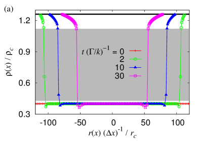
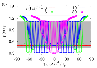
Figure 9: Density profiles extracted from the numerical solutions with the scheme Eq. (C) for (a) Scenario III and (b) Scenario IV. In (a), $\rho^{\rm init}=0.4\rho_{c}$ and $m=1.7m_{0}$ have been used, while $\rho^{\rm init}=0.5\rho_{c}$ and $m=1.7m_{0}$ in (b). Even though the shock waves obtained in this way propagate much faster than in the particle-resolved simulations, the essential features, including the spinodal-like mechanisms for the touching, pair formation, sharp-interface generation, and relaxation to the equilibrium state, are well verified by the numerical solutions. Notably, compared to Fig. 5(a) and Fig. 6, solutions with high density, e.g., $\rho(x)\gtrsim 1.12\rho_{c}$, exhibit much smoother density variations in space, implying an excess numerical diffusion Hirsch (2007) as described in the text.

References

- Filipcsei et al. (2007) G. Filipcsei, I. Csetneki, A. Szilágyi, and M. Zrínyi, Adv. Polym. Sci. 206, 137 (2007).
- Ilg (2013) P. Ilg, Soft Matter 9, 3465 (2013).
- Menzel (2015) A. M. Menzel, Phys. Rep. 554, 1 (2015).
- Odenbach (2016) S. Odenbach, Arch. Appl. Mech. 86, 269 (2016).
- Lopez-Lopez et al. (2016) M. Lopez-Lopez, J. D. Durán, L. Y. Iskakova, and A. Y. Zubarev, J. Nanofluids 5, 479 (2016).
- Frickel et al. (2011) N. Frickel, R. Messing, and A. M. Schmidt, J. Mater. Chem. 21, 8466 (2011).
- Allahyarov et al. (2014) E. Allahyarov, A. M. Menzel, L. Zhu, and H. Löwen, Smart Mater. Struct. 23, 115004 (2014).
- Gundermann and Odenbach (2014) T. Gundermann and S. Odenbach, Smart Mater. Struct. 23, 105013 (2014).
- Landers et al. (2015) J. Landers, L. Roeder, S. Salamon, A. M. Schmidt, and H. Wende, J. Phys. Chem. C 119, 20642 (2015).
- Messing et al. (2011) R. Messing, N. Frickel, L. Belkoura, R. Strey, H. Rahn, S. Odenbach, and A. M. Schmidt, Macromolecules 44, 2990 (2011).
- Roeder et al. (2015) L. Roeder, P. Bender, M. Kundt, A. Tschöpe, and A. M. Schmidt, Phys. Chem. Chem. Phys. 17, 1290 (2015).
- Szabó et al. (1998) D. Szabó, G. Szeghy, and M. Zrínyi, Macromolecules 31, 6541 (1998).
- Volkova et al. (2017) T. Volkova, V. Böhm, T. Kaufhold, J. Popp, F. Becker, D. Borin, G. Stepanov, and K. Zimmermann, J. Magn. Magn. Mater. 431, 262 (2017).
- Schmauch et al. (2017) M. M. Schmauch, S. R. Mishra, B. A. Evans, O. D. Velev, and J. B. Tracy, ACS Appl. Mater. Interfaces 9, 11895 (2017).
- Deng et al. (2006) H. Deng, X. Gong, and L. Wang, Smart Mater. Struct. 15, N111 (2006).
- Sun et al. (2008) T. Sun, X. Gong, W. Jiang, J. Li, Z. Xu, and W. Li, Polym. Test. 27, 520 (2008).
- Bock et al. (2010) N. Bock, A. Riminucci, C. Dionigi, A. Russo, A. Tampieri, E. Landi, V. Goranov, M. Marcacci, and V. Dediu, Acta Biomater. 6, 786 (2010).
- Zhao et al. (2011) X. Zhao, J. Kim, C. A. Cezar, N. Huebsch, K. Lee, K. Bouhadir, and D. J. Mooney, Proc. Natl. Acad. Sci. U.S.A. 108, 67 (2011).
- Müller et al. (2017) R. Müller, M. Zhou, A. Dellith, T. Liebert, and T. Heinze, J. Magn. Magn. Mater. 431, 289 (2017).
- Weeber et al. (2012) R. Weeber, S. Kantorovich, and C. Holm, Soft Matter 8, 9923 (2012).
- Ryzhkov et al. (2015) A. Ryzhkov, P. Melenev, C. Holm, and Y. Raikher, J. Magn. Magn. Mater. 383, 277 (2015).
- Weeber et al. (2015a) R. Weeber, S. Kantorovich, and C. Holm, J. Chem. Phys. 143, 154901 (2015a).
- Weeber et al. (2015b) R. Weeber, S. Kantorovich, and C. Holm, J. Magn. Magn. Mater. 383, 262 (2015b).
- Jarkova et al. (2003) E. Jarkova, H. Pleiner, H.-W. Müller, and H. R. Brand, Phys. Rev. E 68, 041706 (2003).
- Bohlius et al. (2004) S. Bohlius, H. R. Brand, and H. Pleiner, Phys. Rev. E 70, 061411 (2004).
- Annunziata et al. (2013) M. A. Annunziata, A. M. Menzel, and H. Löwen, J. Chem. Phys. 138, 204906 (2013).
- Cerdà et al. (2013) J. J. Cerdà, P. A. Sánchez, C. Holm, and T. Sintes, Soft Matter 9, 7185 (2013).
- Pessot et al. (2014) G. Pessot, P. Cremer, D. Y. Borin, S. Odenbach, H. Löwen, and A. M. Menzel, J. Chem. Phys. 141, 015005 (2014).
- Pessot et al. (2015) G. Pessot, R. Weeber, C. Holm, H. Löwen, and A. M. Menzel, J. Phys.: Condens. Matter 27, 325105 (2015).
- Sánchez et al. (2015) P. A. Sánchez, J. J. Cerdà, T. M. Sintes, A. O. Ivanov, and S. S. Kantorovich, Soft Matter 11, 2963 (2015).
- Ivaneyko et al. (2015) D. Ivaneyko, V. Toshchevikov, and M. Saphiannikova, Soft Matter 11, 7627 (2015).
- Biller et al. (2014) A. M. Biller, O. V. Stolbov, and Y. L. Raikher, J. Appl. Phys. 116, 114904 (2014).
- Biller et al. (2015) A. M. Biller, O. V. Stolbov, and Y. L. Raikher, Phys. Rev. E 92, 023202 (2015).
- Puljiz et al. (2016) M. Puljiz, S. Huang, G. K. Auernhammer, and A. M. Menzel, Phys. Rev. Lett. 117, 238003 (2016).
- Puljiz and Menzel (2017) M. Puljiz and A. M. Menzel, Phys. Rev. E 95, 053002 (2017).
- Menzel (2017) A. M. Menzel, Soft Matter 13, 3373 (2017).
- Heinrich et al. (2011) D. Heinrich, A. R. Goñi, A. Smessaert, S. H. L. Klapp, L. M. C. Cerioni, T. M. Osán, D. J. Pusiol, and C. Thomsen, Phys. Rev. Lett. 106, 208301 (2011).
- Bloom et al. (2012) M. Bloom, S. C. Bae, E. Luijten, and S. Granick, Nature 491, 578 (2012).
- Alvarez and Klapp (2013) C. E. Alvarez and S. H. L. Klapp, Soft Matter 9, 8761 (2013).
- Dobnikar et al. (2013) J. Dobnikar, A. Snezhko, and A. Yethiraj, Soft Matter 9, 3693 (2013).
- Klapp (2016) S. H. Klapp, Curr. Opin. Colloid Interface Sci. 21, 76 (2016).
- An et al. (2010) H. An, S. J. Picken, and E. Mendes, Soft Matter 6, 4497 (2010).
- An et al. (2012) H.-N. An, B. Sun, S. J. Picken, and E. Mendes, J. Phys. Chem. B 116, 4702 (2012).
- Tarama et al. (2014) M. Tarama, P. Cremer, D. Y. Borin, S. Odenbach, H. Löwen, and A. M. Menzel, Phys. Rev. E 90, 042311 (2014).
- Pessot et al. (2016) G. Pessot, H. Löwen, and A. M. Menzel, J. Chem. Phys. 145, 104904 (2016).
- Nadzharyan et al. (2016) T. Nadzharyan, V. Sorokin, G. Stepanov, A. Bogolyubov, and E. Y. Kramarenko, Polymer 92, 179 (2016).
- Pessot et al. (2018) G. Pessot, M. Schümann, T. Gundermann, S. Odenbach, H. Löwen, and A. M. Menzel, J. Phys.: Condens. Matter 30, 125101 (2018).
- Sorokin et al. (2017) V. V. Sorokin, I. A. Belyaeva, M. Shamonin, and E. Y. Kramarenko, Phys. Rev. E 95, 062501 (2017).
- Wood and Camp (2011) D. S. Wood and P. J. Camp, Phys. Rev. E 83, 011402 (2011).
- Melenev et al. (2011) P. Melenev, Y. Raikher, G. Stepanov, V. Rusakov, and L. Polygalova, J. Intel. Mater. Syst. Struct. 22, 531 (2011).
- Zubarev (2013) A. Y. Zubarev, Soft Matter 9, 4985 (2013).
- Romeis et al. (2016) D. Romeis, V. Toshchevikov, and M. Saphiannikova, Soft Matter 12, 9364 (2016).
- Zubarev et al. (2016a) A. Y. Zubarev, L. Y. Iskakova, and M. T. Lopez-Lopez, Physica A 455, 98 (2016a).
- Lopez-Lopez et al. (2017) M. T. Lopez-Lopez, D. Y. Borin, and A. Y. Zubarev, Phys. Rev. E 96, 022605 (2017).
- Gundermann et al. (2017) T. Gundermann, P. Cremer, H. Löwen, A. M. Menzel, and S. Odenbach, Smart Mater. Struct. 26, 045012 (2017).
- Schümann and Odenbach (2017) M. Schümann and S. Odenbach, J. Magn. Magn. Mater. 441, 88 (2017).
- Cremer et al. (2015) P. Cremer, H. Löwen, and A. M. Menzel, Appl. Phys. Lett. 107, 171903 (2015).
- Cremer et al. (2016) P. Cremer, H. Löwen, and A. M. Menzel, Phys. Chem. Chem. Phys. 18, 26670 (2016).
- van Roij (1996) R. van Roij, Phys. Rev. Lett. 76, 3348 (1996).
- Kwaadgras et al. (2013) B. W. Kwaadgras, M. W. J. Verdult, M. Dijkstra, and R. van Roij, J. Chem. Phys. 138, 104308 (2013).
- Zubarev et al. (2016b) A. Y. Zubarev, D. N. Chirikov, D. Y. Borin, and G. V. Stepanov, Soft Matter 12, 6473 (2016b).
- Chaikin and Lubensky (2000) P. M. Chaikin and T. C. Lubensky, Principles of Condensed Matter Physics (Cambridge University Press, Cambridge, 2000).
- Cahn and Hilliard (1958) J. W. Cahn and J. E. Hilliard, J. Chem. Phys. 28, 258 (1958).
- Bates and Fife (1993) P. W. Bates and P. C. Fife, SIAM J. Appl. Math. 53, 990 (1993).
- Elliott and French (1987) C. M. Elliott and D. A. French, IMA J. Appl. Math. 38, 97 (1987).
- Pego (1989) R. L. Pego, Proc. Royal Soc. Lond. A 422, 261 (1989).
- Bialké et al. (2013) J. Bialké, H. Löwen, and T. Speck, Europhys. Lett. 103, 30008 (2013).
- Speck et al. (2014) T. Speck, J. Bialké, A. M. Menzel, and H. Löwen, Phys. Rev. Lett. 112, 218304 (2014).
- Fily et al. (2014) Y. Fily, S. Henkes, and M. C. Marchetti, Soft Matter 10, 2132 (2014).
- Cates et al. (2010) M. E. Cates, D. Marenduzzo, I. Pagonabarraga, and J. Tailleur, Proc. Natl. Acad. Sci. U.S.A. 107, 11715 (2010).
- Stenhammar et al. (2013) J. Stenhammar, A. Tiribocchi, R. J. Allen, D. Marenduzzo, and M. E. Cates, Phys. Rev. Lett. 111, 145702 (2013).
- Wittkowski et al. (2014) R. Wittkowski, A. Tiribocchi, J. Stenhammar, R. J. Allen, D. Marenduzzo, and M. E. Cates, Nat. Commun. 5, 4351 (2014).
- Popescu and Dietrich (2004) M. N. Popescu and S. Dietrich, Phys. Rev. E 69, 061602 (2004).
- Dietrich et al. (2005) S. Dietrich, M. N. Popescu, and M. Rauscher, J. Phys.: Condens. Matter 17, S577 (2005).
- Höllig (1983) K. Höllig, Trans. Am. Math. Soc. 278, 299 (1983).
- Barenblatt et al. (1993) G. I. Barenblatt, M. Bertsch, R. D. Passo, and M. Ughi, SIAM J. Math. Anal. 24, 1414 (1993).
- Witelski (1995) T. P. Witelski, Appl. Math. Lett. 8, 27 (1995).
- Witelski (1996) T. P. Witelski, Stud. Appl. Math. 97, 277 (1996).
- Crank (1975) J. Crank, The Mathematics of Diffusion, 2nd ed. (Oxford University Press, London, 1975).
- Cremer et al. (2017) P. Cremer, M. Heinen, A. M. Menzel, and H. Löwen, J. Phys.: Condens. Matter 29, 275102 (2017).
- Weeks et al. (1971) J. D. Weeks, D. Chandler, and H. C. Andersen, J. Chem. Phys. 54, 5237 (1971).
- Doi and Edwards (1986) M. Doi and S. F. Edwards, The Theory of Polymer Dynamics (Clarendon Press, Oxford, 1986).
- Novick-Cohen and Pego (1991) A. Novick-Cohen and R. L. Pego, Trans. Am. Math. Soc. 324, 331 (1991).
- (84) See Electronic Supplementary Information (ESI) at [URL will be inserted by publisher] for example movies illustrating the dynamic behaviors associated with the different Scenarios I–IV.
- Modica (1987) L. Modica, Arch. Ration. Mech. Anal. 98, 123 (1987).
- Braides (2002) A. Braides, -convergence for Beginners, Oxford Lecture Series in Mathematics, Vol. 22 (Oxford University Press, Oxford, 2002).
- Sandomirski et al. (2011) K. Sandomirski, E. Allahyarov, H. Löwen, and S. U. Egelhaaf, Soft Matter 7, 8050 (2011).
- Huang et al. (2016) S. Huang, G. Pessot, P. Cremer, R. Weeber, C. Holm, J. Nowak, S. Odenbach, A. M. Menzel, and G. K. Auernhammer, Soft Matter 12, 228 (2016).
- Feld et al. (2017) A. Feld, R. Koll, L. S. Fruhner, M. Krutyeva, W. Pyckhout-Hintzen, C. Weiss, H. Heller, A. Weimer, C. Schmidtke, M.-S. Appavou, E. Kentzinger, J. Allgaier, and H. Weller, ACS Nano 11, 3767 (2017).
- Whitham (1999) G. B. Whitham, Linear and Nonlinear Waves (John Wiley & Sons, New York, 1999).
- Patankar (1980) S. Patankar, Numerical Heat Transfer and Fluid Flow (Taylor & Francis, Boca Raton, 1980).
- Hirsch (2007) C. Hirsch, Numerical Computation of Internal and External Flows: The Fundamentals of Computational Fluid Dynamics (Butterworth-Heinemann, Oxford, 2007).