A hierarchical Bayesian model to infer PL(Z) relations using Gaia parallaxes

Abstract

Context. Muraveva et al. (2018a) analysed Period-Luminosity-Metallicity ($PLZ$) relations for RR Lyrae stars using the Gaia Data Release 2 parallaxes. It built on a previous work presented in Gaia Collaboration et al. (2017) that was based on the first Gaia Data Release, and also included Period-Luminosity ($PL$) relations for Cepheids and RR Lyrae stars. The method used to infer the relations in Muraveva et al. (2018a) (and one of the methods used in Gaia Collaboration et al., 2017) was based on a hierarchical Bayesian model, the full description of which was deferred to a subsequent publication that is presented here.

Aims. We aim at creating a Bayesian model to infer the coefficients of $PL$ or $PLZ$ relations that propagates uncertainties in the observables in a rigorous and well founded way.

Methods. We propose a directed acyclic graph to encode the conditional probabilities of the inference model that will allow us to infer probability distributions for the $PL$ and $PL(Z)$ relations. We evaluate the model with several semi-synthetic data sets and apply it to a sample of 200 fundamental mode and first overtone mode RR Lyrae stars for which Gaia DR1 parallaxes and literature $K_{\rm s}$-band mean magnitudes are available. We define and test several hyperprior probabilities to verify their adequacy and check the sensitivity of the solution with respect to the prior choice.

Results. The main conclusion of this work is the absolute necessity of incorporating the existing correlations between the observed variables (periods, metallicities and parallaxes) in the form of model priors in order to avoid systematically biased results, especially in the case of non-negligible uncertainties in the parallaxes. The tests with the semi-synthetic data based on the data set used in Gaia Collaboration et al. (2017) reveal the significant impact that the existing correlations between parallax, metallicity and periods have on the inferred parameters. The relation coefficients obtained here have been superseded by those presented in Muraveva et al. (2018a), that incorporates the findings of this work and the more recent Gaia DR2 measurements.

1 Introduction

Cepheids and RR Lyrae stars are primary standard candles of the cosmological distance ladder because they follow canonical relations that for Cepheids link the star intrinsic luminosity ($L$) to the period ($P$) of light variation, traditionally referred to as period-luminosity relation or Leavitt Law (Leavitt & Pickering 1912; Madore & Freedman 1991; Freedman et al. 2001; Marconi et al. 2005; Saha et al. 2006; Riess et al. 2011, 2016, 2018; Ripepi et al. 2012; Gieren et al. 2013; Gaia Collaboration et al. 2017, hereafter Paper I, and references therein) whereas for RR Lyrae stars link $L$ in the infrared passbands to $P$ and possibly the stellar metallicity ($Z$; $PL$ - metallicity relation – $PL(Z)$; Longmore et al. 1986; Sollima et al. 2006, 2008; Borissova et al. 2009; Marconi et al. 2015; Neeley et al. 2017; Sesar et al. 2017; Muraveva et al. 2018a, b; Paper I and references therein) or $L$ in the visual passband to $Z$ (traditionally referred to as RR Lyrae luminosity - metallicity relation; Cacciari & Clementini 2003, Clementini et al. 2003, Bono et al. 2003, Catelan et al. 2004, Paper I, Muraveva et al. 2018a and references therein). The predicted precision of the Gaia end-of-mission parallaxes for local Cepheids and RR Lyrae stars will allow us to determine the slope and zero point of these fundamental relations with unprecedented accuracy, thus setting the basis for a global reassessment of the whole cosmic distance ladder. As a first anticipation of the Gaia potential in this field of the cosmic distance ladder and a first assessment of improved precision with respect to previous astrometric missions such as, for instance, Hipparcos, and the dramatic increase in statistics compared to what is achievable for instance, measuring parallaxes with the Hubble Space Telescope, Gaia DR1 published parallaxes for more than 700 Galactic Cepheids and RR Lyrae stars, computed as part of the Tycho-Gaia Astrometric Solution (TGAS; Lindegren et al. (2016)). A number of papers after Gaia intermediate data releases in 2016 and 2018 have addressed Cepheids and RR Lyrae stars (e.g. Lindegren et al. 2016; Clementini et al. 2016, 2018; Arenou et al. 2017, 2018) with specific emphasis in their use as standard candles (Casertano et al. 2017; Paper I; Riess et al. 2018; Muraveva et al. 2018a). In Paper I we have used TGAS parallaxes, along with literature photometry and spectroscopy, to calibrate the zero point of the $PL$ relations of classical and type II Cepheids, and the near-infrared $PL$ and $PL(Z)$ relations of RR Lyrae stars by fitting these relations adopting different techniques that operate either in parallax or absolute magnitude space. In that paper different sources of biases affecting the TGAS samples of Cepheids and RR Lyrae stars were discussed at some length and the possible systematic errors caused in the inferred luminosity calibrations were analysed in detail.

Section 3.2 of Paper I in particular discussed the problem of fitting general luminosity relations between the absolute magnitude $M_{\rm True}$, the decadic logarithm of the period $P_{\rm True}$ and possibly also the metallicity $\left[\rm{Fe/H}\right]_{\rm{True}}$ of the form

$$M_{\rm True}=b+c\cdot\log(P_{\rm True})+k\cdot\left[\rm{Fe/H}\right]_{\rm{True}}$$ (1)

with a sample that is truncated in parallax (by removing the non-positive values) and for which the assumption of normality of uncertainties in the absolute magnitude is not valid. A more detailed description of the intricacies involved in using astrometric measurements for the inference of quantities of astrophysical interest in general, and PLZ relation coefficients in particular can be found in Luri et al. (2018). Our proposal in Paper I was to construct a two-level statistical model that distinguishes between true and measured parallaxes. This model can then be used to infer the true parallaxes and absolute magnitudes from the measurements. One of the rigorous ways to construct such a model is to apply the Bayesian methodology where one assigns a prior probability distribution to the true parallax population. In doing so, a suitable selection of this prior will improve the estimation of individual true parallaxes in the sense that their posterior credible intervals are “shrunken” with respect to the measurement uncertainties. Setting a specific prior is always controversial, but in principle it is possible to define only a functional form that depends on a set of unknown parameters. The specific prior is then inferred from the data as part of the global inference process. This prior functional form should be flexible enough to properly model the true distribution of parallaxes but also should be sufficiently restrictive to enforce a plausible distribution for the true parallaxes on the basis of the knowledge present in the astronomical literature.

The solution described in the previous paragraph can be represented as a graph model that incorporates the $PL(Z)$ relation, the definition of absolute magnitudes in terms of the apparent magnitude $m$ and the parallax $\varpi$, and the corresponding distribution of the measurements given the true values. This way we guarantee that the observational uncertainties are simultaneously propagated through the graph and that the uncertainties of the parameters of the $PLZ$ relationship are estimated in a way that is consistent with the measurement uncertainties. Also, the effect of including the relationship

$$b+c\cdot\log P+k\cdot\left[\rm{Fe/H}\right]=m+5\log\varpi-10\,$$ (2)

in the model is to constrain the parameter space in such a way that the $PLZ$ relationship coefficients and the individual true parallaxes have to be consistent.

The objective of this paper is to infer estimates of the parameters of the $PLZ$ relationship. We apply the hierarchical Bayesian methodology, which consists of dividing the variability of the statistical inference problem into several levels. In this way we partition the parameter space associated with inferring the $PLZ$ relation into population-level parameters and observations. We represent the hierarchical Bayesian model with a directed acyclic graph and perform the inference using Markov chain Monte Carlo (MCMC) simulation techniques (Robert & Casella, 2013). A minimal description of the methodology and preliminary results was already presented in Paper I which we intend to extend and clarify here. For reasons of clarity and scope we focus on the inference of the $PLZ$ relationship in the $K$-band for 200 fundamental and first overtone RR Lyrae stars, the main properties of which are provided in Table A.3 of Paper I. The model is applicable with minimal modifications to other variability types such as Cepheids or Long Period Variables and different photometric bands. In this work we present the results of the full model including the slopes of the relation, expanding the results presented in Paper I where only the zero points were inferred while the slopes were fixed to literature values.

A similar methodology has been applied by Sesar et al. (2017) to constrain $PLZ$ relations of fundamental mode (ab type) RR Lyrae stars in the mid-infrared W1 and W2 bands of the Wide-field Infrared Survey Explore (WISE; Wright et al. (2010)), using TGAS parallaxes, but modelling true distances with an exponentially decreasing volume density (hereafter EDVD) prior proposed by Bailer-Jones (2015).

The Bayesian hierarchical method presented in Paper I used a log-normal prior to model the distribution of true parallaxes independently of the other model parameters. With this prior, the $\log\left(P\right)$ slope turned out to be severely underestimated when compared to the literature values, although this result was not specifically discussed therein. In the present work we extend the Bayesian analysis performed in Paper I in three directions. First, we validate the model with semi-synthetic data and analyse the causes of the slope underestimation. Second, we extend the Bayesian analysis by testing alternative prior distributions for parallaxes and demonstrate that one of them mitigates to some degree the problem of the underestimation of the $PLZ$ $\log\left(P\right)$ slope. Third, we study the sensitivity of the Bayesian analysis results under different prior choices for some critical hyperparameters of our hierarchical model (HM).

The structure of the paper is as follows. In Sect. 2 we summarize the theoretical foundations of the hierarchical Bayesian methodology and describe extensively the HM used for inferring the $PLZ$ relationship in Paper I and Muraveva et al. (2018a) (in the latter case with minor adaptations). In Sect. 3 we study the data set in detail and explore its properties by means of semi-synthetic samples constructed assuming a known PLZ relation; in Sect. 4 we present the full results of the MCMC samples of the posterior distribution for the Gaia DR1 data used in Paper I; in Sect. 5 we study the sensitivity of the results to the choice of hyper-parameters, and in Sect. 6 we summarise the findings of the paper.

2 The hierarchical Bayesian model

A full introduction to Bayesian inference and hierarchical Bayes is beyond the scope of this manuscript. We recommend the interested reader to consult Gelman et al. (2004) and Gelman & Hill (2007) for very pedagogic introductions, and Luri et al. (2018) for a more Astronomy-oriented introduction. In what follows, we summarize the main concepts of the methodology. Bayesian inference is based on Bayes’ rule:

$$p\left(\Theta\mid\mathcal{D}\right)\propto p\left(\mathcal{D}\mid\Theta\right)\times p\left(\Theta\right)\,,$$ (3)

where $\mathcal{D}$ are the observations (data), $\Theta$ are the parameters of a model proposed to explain the data and $p$ represents a probability distribution. The right side of Eq. 3 represents the model itself, specified by the joint probability distribution $p\left(\mathcal{D},\Theta\right)$ of the data and the parameters. This distribution factorizes into:

• the conditional distribution $p\left(\mathcal{D}\mid\Theta\right)$ of the data given the parameters (the so called likelihood), and

• the prior distribution of the parameters $p\left(\Theta\right)$, which represents our knowledge about plausible parameter values before observing the data.

The basic model of Eq. 3 divides the variability of the statistical problem into two levels: observations and parameters. The hierarchical Bayesian methodology consists of distinguishing further levels of variability. In our case, we introduce a new dependence of the prior distribution $p\left(\Theta\right)$ on a new set of parameters $\Phi$ (the so called hyperparameters) and assign hyperprior distributions $p\left(\Phi\right)$ to them. We explain its nature in the following sections. In order to have a better understanding of the dependency structure dictated by the model, it is customary to represent the factorization of the joint probability distribution $p\left(D,\mathbf{\Theta},\Phi\right)$ by using the Bayesian network formalism (Pearl, 1988; Lauritzen, 1996), which consists of drawing a DAG (directed acyclic graph) in which nodes encode model parameters, measurements or constants, and directed links represent conditional probability dependence relationships.

The inference in a hierarchical Bayesian model proceeds by calculating the marginal joint posterior distribution of a set of parameters of interest given the data. In complex problems with many parameters the posterior distribution usually is not available in an analytically tractable closed form but can be approximately evaluated using MCMC simulation techniques.

2.1 Conditional dependencies

In this and the next section we describe our sample and the hierarchical model that encodes the conditional probability relations between the observations and the parameters of the linear $PL(Z)$ relations. We include Fig. 19 of Paper I here as Fig. 1, to facilitate reading, but include some additional clarifications that could not be described there due to space and scope limitations.

In the following, we will change the notation to avoid cluttering of subscripts. Henceforth, we will denote measured quantities with a circumflex accent (^) and remove the subscript ${\rm True}$ from the true values. The DAG in Fig. 1 encodes the probabilistic relationships between the variables of our model and shows the measurements at the bottom level: decadic logarithm of periods $\log\hat{P}_{i}$, apparent magnitudes $\hat{m}_{i}$, metallicities $\widehat{\left[\mathrm{Fe/H}\right]}_{i}$, parallaxes $\hat{\varpi}_{i}$ and extinctions $\hat{A}_{m_{i}}$ The subindex $i$ runs from 1 to the total number of stars $N$ in each sample. Our model assumes that the measurements

$$\mathbf{d}_{i}=\left(\hat{m}_{i},\log\hat{P}_{i},\hat{\varpi}_{i},\widehat{\left[\mathrm{Fe/H}\right]}_{i},\hat{A}_{m_{i}}\right)\,,$$ (4)

are realizations from normal distributions centred at the true (unknown) values and with standard deviations given by the measurement uncertainties

$$\bm{\sigma}_{\mathbf{d}_{i}}=\left(\sigma_{m_{i}},\sigma_{\log P_{i}},\sigma_{\varpi_{i}},\sigma_{\left[\mathrm{Fe/H}\right]_{i}},\sigma A_{m_{i}}\right)\,.$$ (5)

Our test sample $\mathcal{D}=\left\{\mathbf{d}_{i}\right\}_{i=1}^{N}$ consists of $N=200$ fundamental mode and first overtone RR Lyrae (RRL) stars with near-infrared (NIR) photometry ($\hat{m}_{i}={\hat{m}}_{K_{s}i}$) selected amongst the stars of the Dambis et al. (2013) compilation for which TGAS parallaxes (Lindegren et al., 2016) and associated uncertainties were available. This is essentially the same $K_{s}$-band sample of Paper I for which the periods of first overtone stars were ”fundamentalised” by adding 0.127 to the decadic logarithm of the period and uncertainties on $\log\left(P\right)$ were estimated as $\sigma_{\log\left(P\right)}=0.01\cdot\log\left(P\right)$ which is equivalent to an uncertainty of 2% in the period. Unlike in Paper I (Sect. 6.1), where metal abundances were transformed from the Zinn & West (1984) to the Gratton et al. (2004) metallicity scale to be consistent with a period term slope of the $PM_{K_{s}}Z$ relationship fixed to the value of $-2.73$ mag/dex reported by Muraveva et al. (2015), in this paper we use the original metal abundances provided by Dambis et al. (2013) because we aim to infer the period term slope. Because Dambis et al. (2013) did not provide metallicity uncertainties, in Paper I we assigned a constant uncertainty of 0.2 dex to all metallicities in the sample. In this paper we distinguish among techniques used to estimate metal abundances and respectively adopt uncertainties of 0.1, 0.2 and 0.3 dex for metallicities estimated from high-resolution spectroscopy, measured by the $\Delta S$ method of Preston (1959) and determined from photometry or other non-spectroscopic methods. The Dambis et al. (2013) catalogue does not include uncertainties on absorption. We estimate them as $\sigma_{A_{K}}=0.114\cdot\sigma_{A_{V}}$ , where $\sigma_{A_{V}}=3.1\cdot\sigma_{E\left(B-V\right)}$ (Cardelli et al., 1989) and $\sigma_{E\left(B-V\right)}=0.16\cdot E\left(B-V\right)$ (Schlegel et al., 1998). All measured quantities are represented as blue nodes in the DAG where we do not include the nodes corresponding to the uncertainties of Eq. 5 in order to facilitate its interpretation.

We represent the likelihood of the model with the nodes corresponding to the true values $m_{i}$, $\varpi_{i}$, $\log P_{i}$, ${\left[\mathrm{Fe/H}\right]}_{i}$ and ${A_{m}}_{i}$ and the arcs going from true values to measurements. True values and observations are all enclosed in a black rectangle that represents replication for the $N$ stars in the sample (plate notation). Equation 1 can be written for every star $i$ in the sample as

$$M_{i}=b+c\cdot\log P_{i}+k\cdot{\left[\mathrm{Fe/H}\right]}_{i}\,,$$ (6)

where $M_{i}$ represents the true absolute magnitude for star $i$. This is a linear model in the parameters: the intercept $b$, the slope $c$ for the period term, and the slope $k$ for the metallicity term. The last term can be dropped if metallicities are thought to play a negligible role in the relationship. We keep it in the following for the sake of completeness, but the particularization to PL relations is straightforward. In Fig. 1 we shadow the left hand rectangle that includes the metallicity terms to remark this choice.

In Fig. 1, the $PL(Z)$ relationship of Eq. 6 is denoted by the grey node $M_{i}$ and all incoming arrows from $c$, $k$, $b$, $P_{i}$ and ${\left[\mathrm{Fe/H}\right]}_{i}$ (that is, the three parameters and two predictive variables). In fact, the reader may have noticed that there is an additional arrow linking $w$ and $M_{i}$. $w$ represents an intrinsic dispersion in the $PL(Z)$ relationship that may be due to evolutionary effects, for example. This dependence on additional predictive variables that are not accounted for in the model is incorporated as an additional Gaussian spread of standard deviation $w$. This spread will be analysed as part of the inference results. Including the additional Gaussian spread that represents unaccounted predictive variables, we have that

$$M_{i}\sim\mathsf{N}\left(b+c\cdot\log P_{i}+k\cdot\left[\mathrm{Fe/H}\right]_{i},w\right)\,,$$ (7)

where $\sim$ should be read as ’is distributed as’, $\mathsf{N}$ represents the normal (Gaussian) distribution, and the comma separates values inside the parenthesis that represent the mean and standard deviation of the normal distribution, respectively.

Figure 1: Directed Acyclic Graph that represents the forward model used to infer the $PLZ$ relation coefficients when the prior of true metallicities, logarithm of true periods and (natural) logarithm of true parallaxes is assumed to be a 3D Gaussian mixture distribution.

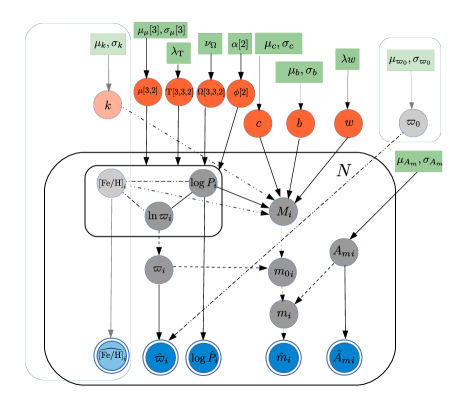
Of course, we do not observe absolute magnitudes, and our model has to account for the transformation between absolute magnitudes and the observations, that are (potentially affected by interstellar absorption) apparent magnitudes. This is shown in the lower part of Fig. 1, where the parallaxes (right-hand block) are handled as we explain next.

The transformation from absolute to unabsorbed apparent magnitudes is a well known deterministic one:

$${m_{0}}_{i}=M_{i}-5\log(\varpi_{i})+10\,,$$ (8)

where the parallax $\varpi_{i}$ is measured in mas. This is not a probabilistic relation and we use dashed lines in the arrows going into ${m_{0}}_{i}$ to distinguish them from the arcs denoting conditional probability links. The absorbed apparent magnitudes are computed as $m_{i}={m_{0}}_{i}+A_{m_{i}}$, where the gray node ${A_{m}}_{i}$ represents the true absorption. The model also contemplates the possibility of a TGAS global parallax offset $\varpi_{0}$. The offset can be inferred by the model or fixed to a predefined value. We shadow the top right rectangle of the graph that includes the offset node to denote this choice.

2.2 Priors, hyperparameters and hyperpriors

Prior distributions allow us to pose probabilistic statements about plausible values of the model parameters based on knowledge available prior to and independent of the observations. But most important, they allow us by means of Bayes’ theorem to make statements about the distribution of the parameters we aim to infer (the posterior distribution of the model parameters in the left side of Equation 3). In the astrophysical context of this paper, we aim at formulating probabilistic statements about the values of the hyperparameters: the most probable value of the $PL(Z)$ slopes or intercepts or their credible intervals. We use green rectangular nodes at the top of the graph to denote fixed prior hyperparameters.

Table 1: Prior ($\pi$) definitions for the hierarchical Bayesian model of the $PL(Z)$ relations. We use the $\pi$ symbol to refer to the prior probability.

$\pi\left(M_{i}\mid b,c,k,w,\log P_{i},{[\rm{Fe/H}]}_{i}\right)=\mathsf{N}\left(b+c\cdot\log\ P_{i}+k\cdot{[\rm{Fe/H}]}_{i},w\right)$

$\pi\left(b\right)=\mathsf{Cauchy}\left(0,10\right)$

$\pi\left(c\right)=\pi\left(k\right)=\mathsf{Cauchy}\left(0,1\right)$

$\pi\left(w\right)=\mathsf{Exp}\left(1\right)$

$\pi\left(\left[\mathrm{Fe/H}\right]_{i},\log P_{i},\ln\varpi_{i}\mid\phi^{\left\{k\right\}},\bm{\mu}^{\left\{k\right\}},\mathrm{T}^{\left\{k\right\}},\Omega^{\left\{k\right\}}\right)=\sum_{k=1}^{2}\phi_{k}\mathsf{MN}\left(\bm{\mu}^{k},\mathrm{T}^{k}\Omega^{k}\mathrm{T}^{k}\right)$

$\pi\left(\bm{\phi}\right)=\mathsf{Dirichlet}\left(1,1\right)$

$\pi\left(\bm{\mu}^{k}\right)=\mathsf{MN}\left(Q_{2k-1}\left(\left[\widehat{\mathrm{Fe/H}}\right],\log\hat{P},\ln\hat{\varpi}\right),\mathrm{diag}\left(0.2^{2},0.1^{2},0.05^{2}\right)\right)$

$\pi\left(\sigma_{Z}^{k}\right)=\pi\left(\sigma_{P}^{k}\right)=\pi\left(\sigma_{\varpi}^{k}\right)=\mathsf{Exp}\left(1\right)$

$\pi\left(\Omega_{P,\varpi}^{k}\right)=\mathsf{LKJ}\left(1\right)$

$\pi\left(\varpi_{0}\right)=\mathsf{N}\left(0,0.1\right)$

Often the prior definitions used in the literature are conservative choices in the sense that they aim to be as non-informative as possible. For both slopes $c$ and $k$ of the $PL(Z)$ relationship of Eq. 6 we specify a standard Cauchy prior (centred at $0$ with scale parameter equal to $1$), which is equivalent to a uniform prior supported on the interval $\left[-\pi/2,+\pi/2\right]$ assigned to the angles $\theta_{1}=\arctan\left(c\right)$ and $\theta_{2}=\arctan\left(k\right)$. The prior probability distribution of the intercept is a Cauchy distribution centred at its mode $\mu_{b}=0$ with scale parameter $\sigma_{b}=10$. The intrinsic dispersion of the $PLZ$ relation is given by an exponential prior with inverse scale $\lambda_{w}=1$.

The only block of the graph that remains to be clarified is the left-hand top block describing the distribution of periods, metallicities and parallaxes. Our model assigns a joint three-dimensional prior to the true distribution of metallicities, periods and parallaxes. Furthermore, we distinguish two components with different chemical composition and a different relationship between pulsation period and parallax (distance). The prior is defined as a mixture of Gaussian distributions (Gaussian mixture, GM) given by

$$\left(\left[\mathrm{Fe/H}\right]_{i},\log P_{i},\ln\varpi_{i}\right)\sim\sum_{k=1}^{2}\phi_{k}\mathsf{MN}\left(\bm{\mu}^{k},\mathrm{T}^{k}\Omega^{k}\mathrm{T}^{k}\right)\,,$$ (9)

where $\phi_{k}$ represents the mixing proportion of the $k$-th component of the mixture, and $\mathsf{MN}$ is a 3D Gaussian probability density with mean vector $\bm{\mu}^{k}=(\mu_{Z}^{k},\mu_{P}^{k},\mu_{\varpi}^{k})$, diagonal matrix of standard deviations $\mathrm{T}^{k}=\mathrm{diag}(\sigma_{Z}^{k},\sigma_{P}^{k},\sigma_{\varpi}^{k})$ and correlation matrix

$$\Omega^{k}=\left(\begin{array}[]{cc}1&\begin{array}[]{cc}0&0\end{array}\\ \begin{array}[]{c}0\\ 0\end{array}&\Omega_{P,\varpi}^{k}\end{array}\right)\,.$$ (10)

The parameters of the prior defined by Equation 9 are themselves model parameters and subject of the Bayesian inference as well. As such, they have their own hyperpriors. We assign a Gaussian prior centred at the first ($Q_{1}$) and third ($Q_{3}$) quartiles of the distribution of the measurements $\left(\left[\widehat{\mathrm{Fe/H}}\right],\log\hat{P},\ln\hat{\varpi}\right)$ and a covariance matrix equal to $\mathrm{diag}\left(0.2^{2},0.1^{2},0.05^{2}\right)$ for the mean vector $\bm{\mu}^{k}$ of each mixture component. This prior is chosen to prevent the non-identifiability of mixture components (the posterior multimodality arising from the fact that swapping the label of the two 3D Gaussian components results in exactly the same solution). We assign a weakly informative exponential prior with inverse scale $\lambda_{\mathrm{T}^{k}}=1$ to the standard deviations in each $\mathrm{T^{k}}$. For each correlation submatrix $\Omega_{P,\varpi}^{k}$ we specify a LKJ prior (Lewandowski et al., 2009) with $\nu=1$ degrees of freedom. The choice of prior given by Equation 9 will prove to be critical for the correct inference of the PLZ relation coefficients for reasons that will become apparent in Sect. 3.

Fig. 1 translates into the following likelihood

$$\begin{split}p\left(\mathcal{D}\mid\mathbf{\Theta}\right)=&\prod_{i=1}^{N}p\left(\mathbf{d}_{i}\mid\mathbf{\Theta}\right)=\prod_{i=1}^{N}p\left(\widehat{[\rm{Fe/H}]}_{i}\mid{[\rm{Fe/H}]}_{i},\sigma_{Z_{i}}\right)\\ &\hphantom{=\prod_{i=1}^{N}}\cdot p\left(\log\hat{P}_{i}\mid\log P_{i},\sigma_{P_{i}}\right)\\ &\hphantom{=\prod_{i=1}^{N}}\cdot p\left(\hat{m}_{i}\mid M_{i},A_{m_{i}},\varpi_{i},\sigma_{m_{i}}\right)\\ &\hphantom{=\prod_{i=1}^{N}}\cdot p\left(\hat{\varpi}_{i}\mid\varpi_{i},\sigma_{\varpi_{i}},\varpi_{0}\right)\\ &\hphantom{=\prod_{i=1}^{N}}\cdot p\left(\hat{A}_{m_{i}}\mid A_{m_{i}},\sigma_{A_{m_{i}}}\right)\end{split}$$ (11)

and priors:

$$\begin{split}\pi\left(\mathbf{\Theta}\right)&=\pi\left(\phi^{\left\{k\right\}},\bm{\mu}^{\left\{k\right\}},\mathrm{T}^{\left\{k\right\}},\Omega_{P,\varpi}^{\left\{k\right\}}\right)\cdot\pi\left(b,c,k,w\right)\cdot\pi\left(\varpi_{0}\right)\\ &\hphantom{=}\cdot\prod_{i=1}^{N}\pi\left(\left[\mathrm{Fe/H}\right]_{i},\log P_{i},\ln\varpi_{i}\mid\phi^{\left\{k\right\}},\bm{\mu}^{\left\{k\right\}},\mathrm{T}^{\left\{k\right\}},\Omega^{\left\{k\right\}}\right)\\ &\hphantom{=\prod_{i=1}^{N}}\cdot\pi\left(M_{i}\mid b,c,k,w,\log P_{i},{[\rm{Fe/H}]}_{i}\right)\\ \end{split}$$ (12)

where each prior probability is defined in Table 1.

We have encoded our HM using the Stan probabilistic modelling language (Carpenter et al., 2017) and used the No-U-Turn sampler (NUTS) of Hoffman & Gelman (2014) to compute the MCMC samples corresponding to the parameters of interests.

3 Model validation with semi-synthetic data.

In this section we aim at validating the improved HM described in Sect. 2 on synthetic data as close as possible to true data sets but following exactly an RR Lyrae $PM_{K_{s}}Z$ relation from the literature. We simulate three sets A, B and C of semisynthetic true absolute magnitudes and parallaxes using that $PM_{K_{s}}Z$ relation and the apparent magnitudes of the sample described in Sect. 2. The only difference between the synthetic data sets A and B lies in the assumed parallax uncertainties. In data set A we generate parallax uncertainties from an hypothesized distribution, and in data set B we use the TGAS uncertainties. No parallax offset is introduced in the simulations. The data set C is identical to data set A except for the uncertainty on metallicity measurements that is reduced by half. Our objective is to analyse the impact of the hyperprior choice, the influence of the parallax and metallicity uncertainties on the inferred coefficients under these three scenarios and detect potential biases in the sample.

3.1 Validation data sets

In what follows, we describe the construction of the three data sets A, B and C that reproduce the generative process of the observations of Eq. 4 from the model hyper-parameters for the three simulated scenarios. In the generation of the semi-synthetic samples we first used a Bayesian model to draw individual true metallicities and logarithms of the true periods from Gaussian posterior distributions inferred from their measurements and associated uncertainties in the real data set described in Sect. 2.2 with vague Gaussian priors assigned to both sets of parameters. Then the observed values were drawn from a Gaussian distribution centred at the true value and with standard deviation given by the measurement uncertainties. For the particular case of data set C the metallicity measurements have been generated dividing by 2 the uncertainties in the real sample. We generated true absolute magnitudes from the $PM_{K}Z$ theoretical calibration of Catelan et al. (2004) adopting $\left[\alpha/\mathrm{Fe}\right]=0.3$ and converting from $\left[\mathrm{Fe/H}\right]$ to $\log Z$ by means of its Eqs. (9) and (10):

$$M_{K_{s}}=-2.353\log P+0.175\left[\mathrm{Fe/H}\right]-0.869.$$ (13)

We generated true parallaxes from

$$\varpi_{i}=10^{2+0.2\left(M_{i}-{m_{0}}_{i}\right)}\,,$$ (14)

where ${m_{0}}_{i}$ is the unabsorbed apparent magnitude of the $i$-th star in the real sample. For data set A we generated measured parallaxes from a Gaussian distribution centred at the true parallaxes given by Eq. 14 with standard deviations drawn from an exponential distribution with inverse scale parameter equal to $10$ plus a zero-point of 0.01 mas. We note that the uncertainties on TGAS parallaxes are higher than these ones by approximately one order of magnitude, but our objective here is to evaluate the performance of our HM under the small uncertainties typical of the Gaia DR2. The measured parallaxes of data set B were generated using the TGAS parallax uncertainties.

Figure 2: Plot of the observed absolute magnitudes as a function of the true decadic logarithm of the period for simulations A and B The red solid line represents the projection of the $PM_{K_{s}}Z$ relation of Eq. 13 for a value of the true metallicity equal to the median of the values generated according to the text. Colours encode the simulated true parallaxes according to the logarithmic scale on the right.

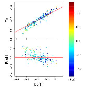
Figure 2 represents in the top panel the values of the absolute magnitudes and logarithms of the true periods generated for simulations A and B. The red line shows the PL relation for the median value of $[\rm{Fe/H}]$ in the simulated sample. Because this plot is a 2D projection of the 3D $PM_{K_{s}}Z$ relation and the absolute magnitudes were sampled from it, any deviations from the red line can only be explained by metallicities differing from the median and the intrinsic dispersion of the relation (which is symmetric). A correlation between periods and metallicities is evident which results in correlated residuals (lower panel) with respect to the assumed PL for the median true metallicity. We also observe in the figure a correlation with the distance: brighter magnitudes correspond (on average) to longer periods and lower metal abundances at larger distances (lower parallaxes) and viceversa. Figure 3 demonstrates that the correlation between periods, metallicities and parallaxes is not an added effect in the simulations and is present in the measurements both for the simulated and the real data set. The figure represents the measured metallicities vs. the logarithm of the period for simulations A and B and for the real sample. The colour code reflects the natural logarithm of the parallaxes: the same true value for simulations A and B in the top panel, the observed value for simulation B in the middle panel, and the measured value of the TGAS catalogue in the bottom panel. The black crosses denote the first and third quartiles of the marginal distributions along each axis. In principle, one expects the distribution of periods to be independent of distance. However, Fig. 3 shows that the left half of the plot (stars with short periods) is predominantly populated by stars with larger parallaxes and higher metallicities while the right half is, again on average, predominantly populated by distant stars (smaller parallaxes) with lower metallicities. We observe that the correlation between the simulated true parallaxes, measured periods and metallicities shown by the top panel of the figure persists for the measured parallaxes depicted in the middle panel, although with larger dispersion due to the higher parallax uncertainties of simulation B. We also note that the correlation is also present in the real sample of TGAS parallaxes (bottom panel). The interpretation is as follows: we expect nearby stars in our sample to be characterised on average by the higher metallicities of the disk, while the opposite is true for those further away in the halo. This dependence of distance on metallicity is visible in the colour code of Fig. 3 and crudely characterized by the two black crosses on each panel. Each cross represents the projection of the point $Q_{k}\left(\left[\mathrm{Fe/H}\right],\log P,\ln\omega\right)$ (with $Q_{k}$ denoting the $k$-th quartile for $k=1,2$ ) onto the period-metallicity plane. The crosses on the top panel of the figure correspond respectively to distances of $1.87$ and $1.07$ kpc for a lower ($-1.72$ dex) and higher ($-1.11$ dex) metallicity component.

Figure 3: Scatter plot of observed metallicities and $\log(P)$ for validation sets A and B and the real sample used in the paper. The black crosses represent the first ($Q_{1}$) and third ($Q_{3}$) quartile of the distribution of measured $\log(P)$ and ${[\rm{Fe/H}]}$ for simulations A and B (top and middle panel) and the real sample (bottom panel). The colour encodes the natural logarithm of true parallaxes of simulations A and B (top panel), measured parallaxes of simulation B (middle panel) and TGAS parallax estimates (bottom panel).

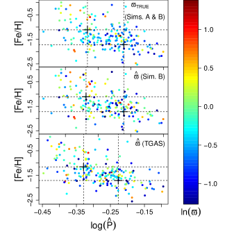
The correlations just described show themselves on the period luminosity diagram of Fig. 2 in the following way. Because higher metallicities correspond to shorter periods (as illustrated in Fig. 3) we then expect the nearby stars (that let us recall, are on average more metal-rich) to be characterised by shorter periods (the left half of the PL diagram). And the opposite is also true: the distant (small parallax) halo stars have on average lower metallicities and hence, longer periods (the right half of the PL diagram). This scenario is then prone to systematic biases in the $\log(P)$ slope inference results because it is precisely at the right edge of the PL diagram that there is a concentration of the most distant sources that will inevitably be characterised by larger fractional parallax uncertainties. We know that in general, the prior plays a minor role whenever the uncertainties are small because a narrow likelihood dominates the posterior. And the opposite is true for stars with large fractional parallax uncertainties: the likelihood is barely informative and it is the prior that dominates the posterior. Bailer-Jones (2015) shows very pedagogic illustrations of this for the problem of inferring distances for parallaxes under several prior specifications. In our case, the stars for which the prior has a larger impact on the inference of the parallax are predominantly placed at the rightmost range of periods.

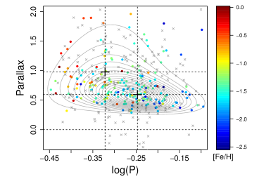
These relatively hidden correlations will have important consequences for the inference as we will see. In particular, it will have an impact on the choice of prior. In general, the parallax prior has to have support (non-vanishing values) in all the range of true parallaxes. But this is even more important given the correlation between periods and true parallaxes because in the case of our simulations, long periods have on average the smallest parallaxes. If the prior has zero probability density for the small true parallaxes, and given the relatively large parallax uncertainties in our sample, the model will systematically assign parallaxes larger than the true ones (will overestimate them). Given that in both simulated data sets, the full range of absolute magnitudes is reduced to a brighter magnitude range for lower parallaxes, and because the strong deterministic relationship between absolute magnitudes and true parallaxes established by Eq. 8 of the HM, the model will infer absolute magnitudes fainter than the true (brighter) ones. Finally, if the stars with long periods get fainter absolute magnitudes, the model will systematically underestimate the absolute value of the period slope coefficient of the $PLZ$ relation. Hence, if our interpretation is correct, the distance prior has to be made dependent on metallicity. The model described in Sect. 2 addresses this problem by using a 3D prior that distinguishes between two probabilistic classes of metal abundance in the data and constrains the true parallaxes of each class by means of their relationship with periods. Figure 4 shows an example of our 3D GM prior fitted to the distribution of true $\left(\left[\mathrm{Fe/H}\right],\log P,\ln\varpi\right)$ in simulation B using a Bayesian HM. The figure represents the projection of the fitted probability density function (PDF) onto the plane period-parallax (with the parallax represented in linear scale) and depicts the measured pairs $\log(P)$-parallax in the simulated dataset. We note that without a proper modelling of the selection effect that gives rise to the correlation between periods and true parallaxes, the inference will return a severely underestimated $\log(P)$ slope, as we will demonstrate towards the end of this section, where our model will be compared with a model that uses 1D independent prior distributions for period, metallicity and parallax. This comparison will illustrate the shrinkage power of hierarchical models.

Figure 4: Projection of a two components 3D GM PDF fitted to the true values of $\left(\left[\mathrm{Fe/H}\right],\log P,\ln\varpi\right)$ in the data set B onto the plane period-parallax. The gray contours represent iso-probability lines. The coloured and gray points represent respectively true and measured parallaxes. The black crosses indicate the median of the mean posterior distribution of each GM component. The colour encodes the metallicity.

3.2 Validation results

Figure 5 compares the parallaxes inferred by our HM with the true ones simulated for datasets A (top panel) and B (bottom panel). The colours in both panels represent the $\log(P)$ according to the colour scale to the right. For simulation B we observe that lower parallaxes (typical of the longer periods) are slightly overestimated. We also observe that the smallest (and overestimated) parallaxes correlate as expected with longer periods. But the largest parallax overestimations do not correspond systematically to the longest periods which is guaranteed by the 3D prior used in our HM. The overestimation of the smallest parallaxes is interpreted as a deficiency of our Gaussian 3D prior that fails to represent adequately the more complex spatial distribution of RR Lyrae stars in the Galaxy.

Figure 5: Comparison between inferred and true parallaxes for validation sets A and B. The solid lines represent the bisectors and the colour encodes the value of the decadic logarithm of the period in days according to the colour scale on the right.

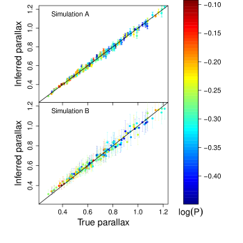
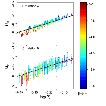
Figure 6 compares, for simulations A and B, the inferred absolute magnitudes with the true periods and represents the $PM_{K}Z$ relation inferred in each case. Table 2 summarises the coefficients of the resulting $PM_{K}Z$ relations providing 68% credible intervals around the median of the posterior distributions of them. For simulation B (bottom panel of Fig.6) we observe that brighter magnitudes are slightly underestimated for long period stars. This mild bias is not present for the data set A (upper panel) because the negligible parallax uncertainties tightly constrain the model parameters (the true parallaxes and hence, the absolute magnitudes and the slopes of the relation). To better appreciate this results we suggest the reader also compare the inferred absolute magnitudes of the two scenarios of Fig. 6 with their simulated values on Fig. 2. The mild underestimation of brighter magnitudes for simulation B translated into a mild underestimation of the inferred $\log(P)$ slope (second row of Table 2) with a credible interval of ${-2.13}_{-0.78}^{+0.75}$ mag/dex which in any case is in good agreement with the value $c=-2.35$ used for the simulation taken into account the large parallax uncertainties in this case. For simulation A the credible interval obtained for the $\log(P)$ slope was ${-2.48}_{-0.14}^{+0.15}$ mag/dex which slightly overestimate $c=-2.35$. We hypothesize that this mild overestimation of the $\log(P)$ slope is a consequence of the correlation between period and metallicity and the relatively large uncertainties of measured metallicities. In order to evaluate this hypothesis we have used the third semi-synthetic data set (labelled C) whose uncertainties on simulated metallicity measurements are of the order of magnitude typical for high-resolution spectroscopic techniques. The results for simulation C are included in the bottom row of Table 2 and seem to confirm our intuition.

Figure 6: Comparison between inferred absolute magnitudes and true periods for validation sets A and B. The black-solid and red-dashed lines represent respectively the projections of the $PM_{K}Z$ relation of Eq. 13 and the relation inferred by our HM (adopting the median value of the posterior distribution of each coefficient) for a value of the true metallicity equal to the median of the values generated according to the text. The colour encodes the metallicity according to the scale on the right.

Table 2: Coefficients of the $PM_{K}Z$ relations inferred from the measurements of simulations A, B and C: slopes ($c$ and $k$), zero-point ($b$) and intrinsic dispersion ($w$). The posterior distribution of coefficients is summarized by the median plus minus the difference in absolute value between the median and the 84th and 16th percentile (first line) and the maximum a posteriori (MAP) estimate (second line) for each simulation.

Simulation	$c$	$k$	$b$	$w$
	(mag/dex)	(mag/dex)	(mag)	(mag)
A	${-2.48}_{-0.14}^{+0.15}$	${0.15}_{-0.02}^{+0.03}$	${-0.93}_{-0.06}^{+0.07}$	${0.03}_{-0.01}^{+0.02}$
	$-2.51$	$0.15$	$-0.94$	$0.03$
B	${-2.13}_{-0.78}^{+0.75}$	${0.22}_{-0.10}^{+0.10}$	${-0.72}_{-0.31}^{+0.31}$	${0.20}_{-0.07}^{+0.07}$
	$-2.03$	$0.22$	$-0.71$	$0.21$
C	${-2.39}_{-0.14}^{+0.15}$	${0.17}_{-0.03}^{+0.02}$	${-0.89}_{-0.07}^{+0.07}$	${0.03}_{-0.071}^{+0.02}$
	$-2.39$	$0.17$	$-0.88$	$0.03$

Table 3: Coefficients of the $PM_{K}Z$ relations inferred for the simulated scenarios A and B by an HM using the 3D GM prior and two 1D parallax priors (the log-normal prior used in Paper I and the EDVD prior of Bailer-Jones (2015)): slopes ($c$ and $k$), zero-point ($b$) and intrinsic dispersion ($w$). The posterior distribution of each coefficient is summarized as in Table 2.

Simulation	Prior	$c$	$k$	$b$	$w$
		(mag/dex)	(mag/dex)	(mag)	(mag)
	3D GM	${-2.48}_{-0.14}^{+0.15}$	${0.15}_{-0.02}^{+0.03}$	${-0.93}_{-0.06}^{+0.07}$	${0.03}_{-0.01}^{+0.02}$
		$-2.51$	$0.15$	$-0.94$	$0.03$
A	EDVD	${-2.46}_{-0.15}^{+0.16}$	${0.16}_{-0.03}^{+0.03}$	${-0.92}_{-0.07}^{+0.08}$	${0.03}_{-0.01}^{+0.02}$
		$-2.48$	$0.15$	$-0.92$	$0.03$
	Log-Normal	${-2.46}_{-0.15}^{+0.16}$	${0.15}_{-0.03}^{+0.03}$	${-0.93}_{-0.07}^{+0.07}$	${0.04}_{-0.01}^{+0.02}$
		$-2.47$	$0.15$	$-0.94$	$0.03$
	3D GM	${-2.13}_{-0.78}^{+0.75}$	${0.22}_{-0.10}^{+0.10}$	${-0.72}_{-0.31}^{+0.31}$	${0.20}_{-0.07}^{+0.07}$
		$-2.03$	$0.22$	$-0.71$	$0.21$
B	EDVD	${-1.31}_{-0.67}^{+0.63}$	${0.12}_{-0.10}^{+0.10}$	${-0.62}_{-0.29}^{+0.28}$	${0.18}_{-0.06}^{+0.07}$
		$-1.32$	$0.12$	$-0.62$	$0.17$
	Log-Normal	${-0.95}_{-0.63}^{+0.59}$	${0.08}_{-0.10}^{+0.10}$	${-0.52}_{-0.27}^{+0.26}$	${0.24}_{-0.06}^{+0.06}$
		$-0.87$	$0.10$	$-0.50$	$0.25$

Table 3 compares the results obtained with the 3D GM prior discussed above with those of alternative 1D priors based on the log-normal prior used in Paper I and the EDVD prior of Bailer-Jones (2015) given by Equation 15.

$$p\left(\varpi\right)=\frac{1}{2L^{3}\varpi^{4}}\exp\left(-\frac{1}{\varpi L}\right)\,.$$ (15)

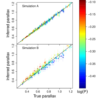
It shows that the existing correlations amongst periods, parallaxes and metallicities have a small impact in the context of the small parallax uncertainties that characterise simulation A, but affect (worsen) significantly the inference outcome for the typical TGAS uncertainties. Figure 7 illustrates these facts by comparing the parallaxes inferred by an HM with an EDVD prior with the true parallaxes of both semi-synthetic data sets A and B. We observe that in simulation B (bottom panel) the overestimation and underestimation of the inferred parallaxes is severe as compared to Fig. 5 of Sect. 3.

It is important to bear in mind that although succesive Gaia data releases will tend to decrease the measurement uncertainties in general, the community will often work with samples of stars (not necessarily classical pulsators like in the case of Paper I; Muraveva et al. 2018a) with Gaia uncertainties in the range exemplified by our TGAS sample.

Figure 7: Comparison between inferred and true parallaxes for validation sets A and B when a HM with an EDVD prior is used. The colour encodes the value of the decadic logarithm of the period in days according to the colour scale on the right.

4 Application to the RR Lyrae Gaia DR1 data

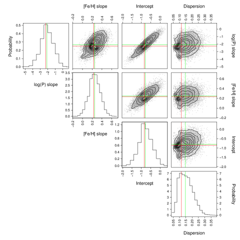
Table 4 presents summary statistics associated with the $PM_{K}Z$ relationships obtained by our HM trained with the RR Lyrae sample described in Sect. 2 for the cases of a potential TGAS global parallax offset inferred by the model or fixed to literature values. Figure 8 shows the MCMC posterior samples (in 2D projections) of the relationship parameters for the model with inferred offset. The black contours in the figure represent iso-probability lines. We see clear correlations between the three strong parameters (two slopes and the intercept). The posterior medians of the $\log(P)$ slope, the metallicity slope and the intercept are, respectively, $-2.1$ mag/dex, $+0.25$ mag/dex and $-0.79$ mag (top portion of Table 4). The inferred period slope is consistent with the values reported in the literature both for empirical and theoretical studies (see Table 3 of Muraveva et al. (2015)). The metallicity slope is systematically higher than the values reported from empirical studies but is in good agreement with the theoretical calibrations of Bono et al. (2003) and Catelan et al. (2004). The posterior median of the intrinsic width is $0.15$ mag. The credible interval of the parallax offset $\varpi_{0}=+0.014\pm 0.032$ is in disagreement with the negative estimate $\varpi_{0}=-0.036\pm 0.002$ of Arenou et al. (2017) but is consistent with the MAP estimate $\varpi_{0}=+0.02$ inferred by the probabilistic approach of Sesar et al. (2017) using $W2$-band RR Lyrae data. In any case we explain a hypothetical overtestimation (towards positive values) of the global parallax offset inferred by our HM model as follows. As we showed in Sect. 3.2 the model with 3D GM prior mitigates the systematic overstimation of smaller parallaxes for longest periods in a scenario of large parallax uncertainties. As a consequence of this the lowest parallaxes inferred by the model are, on average, smaller that their measurements (with the obvious exception of parallaxes with negative measurements), which in turn leads to a positive offset estimate. We stress that the parallax offset reported in this paper should no to be used as a reliable estimate of the potential TGAS offset. On the contrary, the global parallax offset $\varpi_{0}=-0.057$ reported in Muraveva et al. (2018a) for Gaia DR2 was inferred from a scenario of sufficiently precise parallax uncertainties in which the parallax prior played a relatively minor role, hence, is in principle more reliable.

The bottom portion of Table 4 presents the $PLZ$ relationship parameters inferred by our HM with a global parallax offset fixed to the value $\varpi_{0}=-0.036$ mas estimated by Arenou et al. (2017). We do not observe major differences in the slopes with regard to those obtained by the HM based on the inferred offset of $+0.014$ mas (see top portion of the table). Nevertheless, the difference between the intercepts is equal to 0.11 mag, which translates into a Large Magellanic Cloud (LMC) distance modulus $0.09$ mag longer than inferred by the model with offset fixed to $\varpi_{0}=-0.036$ mas. The distance moduli have been estimated from a sample of 70 RRLs located close to the LMC bar, with photometry in the $K_{s}$-band and spectroscopically measured metallicities (described and used in Paper I; Muraveva et al. 2018a).

Figure 8: Marginal posterior distributions from the MCMC samples of the $PM_{K}Z$ relationship parameters for our HM with the potential TGAS parallax offset included as a model parameter. The diagonal shows the uni-dimensional marginal distributions for the slope of the $\log(P)$ term in the linear relation, the slope of the metallicity term, the intercept and the intrinsic dispersion of the relationship. Green and red lines point respectively towards the median and the MAP estimate of each one-dimensional posterior marginal distribution.

Table 4: Coefficients of the $PM_{K}Z$ relation inferred from the real RRL sample described in Sect. 2: slopes ($c$ and $k$), zero-point ($b$), intrinsic dispersion ($w$) , global parallax offset ($\varpi_{0}$) and LMC distance modulus ($\mu_{\rm LMC}$) . The posterior distribution of each coefficient is summarized as in Table 2.

$c$	$k$	$b$	$w$	$\varpi_{0}$	$\mu_{\rm LMC}$
(mag/dex)	(mag/dex)	(mag)	(mag)	(mas)	(mag)
${-2.10}_{-0.75}^{+0.87}$	${0.25}_{-0.11}^{+0.12}$	${-0.79}_{-0.32}^{+0.36}$	${0.15}_{-0.05}^{+0.06}$	${+0.014}_{-0.032}^{+0.032}$	${18.73}_{-0.11}^{+0.11}$
$-2.26$	$0.23$	$-0.85$	$0.12$	$+0.013$	$-$
${-2.04}_{-0.72}^{+0.77}$	${0.25}_{-0.11}^{+0.11}$	${-0.68}_{-0.31}^{+0.33}$	${0.16}_{-0.06}^{+0.06}$	${-0.036}$	${18.64}_{-0.11}^{+0.11}$
$-2.05$	$0.25$	$-0.71$	$0.16$	$-$	$-$

Figure 9: Comparison between the TGAS parallaxes and the maximum a posteriori estimates from the hierarchical model (HM). The error bars correspond to the TGAS parallax uncertainties (horizontal) and credible intervals calculated as the median plus minus the difference between the median and the 84th and 16th percentile (vertical). The red circles correspond to stars with parallax difference beyond 2 times the combined uncertainties.

Figure 9 shows a comparison between the parallaxes catalogued in TGAS and the posterior estimates of our hierarchical model. The horizontal error bars represent TGAS uncertainties and the vertical ones are given by 68% credible intervals calculated around the median of the marginal posterior distributions. We see that our hierarchical model is capable of reducing (“shrinking”) the uncertainties using the constraint that the absolute magnitudes must follow a linear relationship with (the logarithm of the) periods and metallicities with a slope in agreement with previous estimates. The median of the standard deviations of the posterior samples is 0.07 mas with a maximum value of 0.2, which is the minimum value of the TGAS parallax uncertainties. As shown in Fig. 9, the maximum uncertainties of the MCMC parallax samples correspond to the same stars with minimum TGAS uncertainties (those with maximum TGAS parallax measurements). This means that the hierarchical model is not capable of significantly improving the parallax uncertainties of the stars near the Sun. We also see that there are stars with TGAS and HM parallaxes that disagree beyond the error bars. We plot in red stars that are 2-3 standard deviations away from the diagonal (as measured in the 2D plane of Fig. 9 by the Mahalanobis distance $\sqrt{(\mathbf{x}-\bm{\mu})^{T}\mathbf{\Sigma}^{-1}(\mathbf{x}-\bm{\mu})}$, where $\mathbf{x}$ is the vector ($\varpi_{\rm TGAS}$,$\varpi_{\rm HM}$) and $\bm{\mu}$ is the perpendicular projection of $\mathbf{x}$ onto the diagonal).

Figure 10: Left. Samples of the $PLZ$ relations derived from the MCMC samples for ${[\rm{Fe/H}]}=-1.46$ (the median of the distribution of inferred metallicities) (grey lines) and period-$M_{\rm K}$ values inferred by the HM and computed according to Eq. 16. Right. As in the left panel, but with $M_{\rm K}$ computed according to Eq. 17. The colour encodes the inferred metallicity according to the scale on the right.

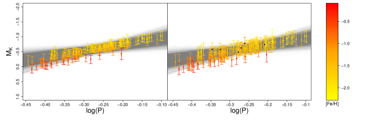
Figure 10 shows the PL relations derived from the HM. Each grey line corresponds to one sample in the Markov chain. All $PM_{K}Z$ relations have been particularized to a value of the metallicity ${[\rm{Fe/H}]}=-1.46$ dex, which is the median of the distribution of inferred values. On the left hand panel we show the values of the absolute magnitude in the $K$ band derived from the MCMC samples as

$$M_{\rm K}^{i,n}=c^{n}\cdot\log(P^{i,n})+k^{n}\cdot{[\rm{Fe/H}]}^{i,n}+b^{n}\,,$$ (16)

where the superindex $i$ tags stars (from 1 to $N$) and the superindex $n$ tags the sample in the MCMC set of samples. In the right hand panel we show the same diagram, but computing the absolute magnitude from the measured apparent magnitude and the MCMC parallax:

$$M_{\rm K}^{i,n}=\hat{m}_{0}^{i}+5\cdot\log(\varpi^{i,n})-10\,,$$ (17)

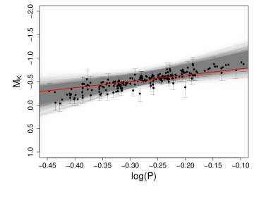
where $\hat{m}_{0}^{i}$ represents the measured value of the apparent magnitude corrected for the measured absorption (that is, we only use the parallaxes from the model, but the absorptions and apparent magnitudes used in Eq. 17 are the measured values in the sample described in Sect. 2 . The black circles correspond to the discrepant sources marked by red circles in Fig. 9. The outlier at $\log(P)\approx-0.26$ corresponds to V363 Cas. This star was classified as a double-mode pulsator by Hajdu et al. (2009). A detailed analysis of its nature is beyond the scope of this paper, but we note that it would be consistent with its discrepant position in the diagrams. The two panels of Fig. 10 can be compared to the period-absolute magnitude diagram of Fig. 11 in which the absolute magnitudes were predicted from a $PLZ$ relation whose coefficients were estimated fitting by weighted non-linear least squares the following model

$$\hat{\varpi}10^{0.2\hat{m}_{0}-2}=10^{0.2\left(c\log\hat{P}+k\left[\widehat{\mathrm{Fe/H}}\right]+b\right)}\,,$$ (18)

where the dependent variable $\alpha=\hat{\varpi}10^{0.2\hat{m}_{0}-2}$ in the left side of Eq. 18 is the Astrometry-Based Luminosity (ABL) defined by Arenou & Luri (1999) with $\hat{\varpi}$ denoting the TGAS parallax. The red line in Fig. 11 represents the projection of the $PLZ$ relation derived by this method for a value of the metallicity equal to its median in the sample. The $\log(P)$ slope, metallicity slope and intercept estimates were respectively $c=-1.34\pm 0.95$ mag/dex, $k=0.20\pm 0.13$ mag/dex and $b=-0.62\pm 0.40$ mag.

Figure 11: $PLZ$ relations defined by the MCMC samples for the value of ${[\rm{Fe/H}]}=-1.46$ (dark grey lines) and the measured periods, and absolute magnitudes predicted by using the ABL method described in the text. The red line represents the projection of the $PLZ$ relation used for predictions for a value of the metallicity equal to its median in the sample.

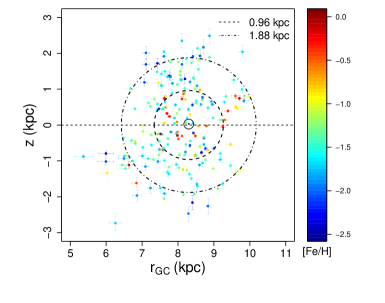
One of the advantages of addressing the problem of calibrating a $PL(Z)$ relationship by means of a Bayesian HM is the ability to infer the posterior distribution of any parameter of interest. In particular we aimed to derive individual heliocentric distances to the RRL stars in our sample and locate their positions in the Galaxy. For that, the measured coordinates $(\alpha,\delta)$ of our RRL stars were first transformed to Galactic coordinates $(l,b)$. Then, for each RR Lyrae we derived samples of the posterior distribution of its rectangular coordinates $(x_{i},y_{i},z_{i})$ from samples of its posterior parallax ($\varpi_{i}$) in the Cartesian Galactocentric coordinate system of Jurić et al. (2008) by

$$\begin{split}x_{i}^{n}&=R_{\odot}-d_{i}^{n}\cos\left(l_{i}\right)\cos\left(b_{i}\right)\\ y_{i}^{n}&=-d_{i}^{n}\sin\left(l_{i}\right)\cos\left(b_{i}\right)\\ z_{i}^{n}&=d_{i}^{n}\sin\left(b_{i}\right)\,,\\ \end{split}$$ (19)

where $d_{i}^{n}=1/\varpi_{i}^{n}$ denotes the posterior distance calculated as the reciprocal of the posterior parallax and $R_{\odot}=8.3$ kpc is the adopted distance to the Galactic centre (Gillessen et al., 2009). The samples of the posterior distribution of the radial distance of each star to the Galactic centre were calculated as

$${r_{\mathrm{GC}}}_{i}^{n}=\sqrt{\left(x_{i}^{n}\right)^{2}+\left(y_{i}^{n}\right)^{2}}\,.$$ (20)

Figure 12 represents the spatial distribution and metal abundance of our RR Lyrae sample in the plane $z-r_{\mathrm{GC}}$ associated with the Galactocentric reference frame. Each Sun-centred circumference in the figure corresponds to Galactocentric coordinates calculated from the Galactic longitudes $l=0^{\circ}$ and $l=180^{\circ}$ (at any Galactic latitude) and the distances corresponding to the median of the mean log-parallax posterior distribution associated with each Gaussian mixture component of our HM.

Figure 12: Spatial distribution and metallicity of the RR Lyrae sample used in this paper represented in a Galactocentric reference frame. $r_{\rm GC}$ and $z$ denote respectively the radial distance to the Galactic centre (GC) and the vertical distance with regard to the Galactic midplane $x-y$. The Cartesian Galactocentric coordinates and the radial distances to the GC have been summarized by the median plus minus the difference in absolute value between the median and the 84th and 16th percentile of the posterior samples of Eqs. 19 and 20.

Table 5: Summary statistics corresponding to the sensitivity analysis performed to the HM with joint 3D GM prior presented in this paper: slopes ($c$ and $k$), zero-point ($b$), intrinsic dispersion ($w$) and global parallax offset ($\varpi_{0}$). The posterior distribution of each coefficient is summarized as in Table 2.

Prior	$c$	$k$	$b$	$w$	$\varpi_{0}$
	(mag/dex)	(mag/dex)	(mag)	(mag)	(mas)
$\pi\left(c\right)=\pi\left(k\right)=\mathsf{Cauchy}\left(0,\sigma=2.5\right)$	$-2.23\begin{subarray}{c}+0.78\\ -0.77\end{subarray}$	$+0.24\begin{subarray}{c}+0.12\\ -0.11\end{subarray}$	$-0.83\begin{subarray}{c}+0.33\\ -0.34\end{subarray}$	$0.16\begin{subarray}{c}+0.06\\ -0.05\end{subarray}$	$+0.015\begin{subarray}{c}+0.035\\ -0.035\end{subarray}$
	$-2.22$	$+0.24$	$-0.83$	$0.15$	$+0.015$
$\pi\left(w\right)=\mathsf{Exp}\left(\lambda=0.1\right)$	$-2.05\begin{subarray}{c}+0.81\\ -0.81\end{subarray}$	$+0.26\begin{subarray}{c}+0.11\\ -0.11\end{subarray}$	$-0.75\begin{subarray}{c}+0.35\\ -0.35\end{subarray}$	$0.16\begin{subarray}{c}+0.05\\ -0.06\end{subarray}$	$+0.012\begin{subarray}{c}+0.035\\ -0.033\end{subarray}$
	$-2.06$	$+0.26$	$-0.74$	$0.15$	$+0.008$
$\pi\left(w\right)=\mathsf{Exp}\left(\lambda=1\right)$	$-2.10\begin{subarray}{c}+0.87\\ -0.75\end{subarray}$	$+0.25\begin{subarray}{c}+0.12\\ -0.11\end{subarray}$	$-0.79\begin{subarray}{c}+0.36\\ -0.32\end{subarray}$	$0.15\begin{subarray}{c}+0.06\\ -0.05\end{subarray}$	$+0.014\begin{subarray}{c}+0.032\\ -0.032\end{subarray}$
	$-2.26$	$+0.23$	$-0.85$	$0.12$	$+0.013$
$\pi\left(w\right)=\mathsf{Exp}\left(\lambda=10\right)$	$-2.10\begin{subarray}{c}+0.76\\ -0.78\end{subarray}$	$+0.25\begin{subarray}{c}+0.11\\ -0.11\end{subarray}$	$-0.79\begin{subarray}{c}+0.32\\ -0.33\end{subarray}$	$0.12\begin{subarray}{c}+0.05\\ -0.04\end{subarray}$	$+0.015\begin{subarray}{c}+0.032\\ -0.032\end{subarray}$
	$-2.13$	$+0.23$	$-0.69$	$0.12$	$+0.016$
$\pi\left(\bm{\mu}^{k}\right)$ with $\sigma_{\mu_{\varpi}}^{k}=0.1$	$-1.92\begin{subarray}{c}+0.81\\ -0.69\end{subarray}$	$+0.21\begin{subarray}{c}+0.11\\ -0.10\end{subarray}$	$-0.63\begin{subarray}{c}+0.35\\ -0.30\end{subarray}$	$0.16\begin{subarray}{c}+0.06\\ -0.05\end{subarray}$	$-0.006\begin{subarray}{c}+0.039\\ -0.040\end{subarray}$
	$-2.08$	$+0.20$	$-0.78$	$0.15$	$-0.008$
$\pi\left(\bm{\mu}^{k}\right)$ with $\sigma_{\mu_{\varpi}}^{k}=0.5$	$-1.60\begin{subarray}{c}+0.81\\ -0.69\end{subarray}$	$+0.17\begin{subarray}{c}+0.11\\ -0.11\end{subarray}$	$-0.64\begin{subarray}{c}+0.32\\ -0.33\end{subarray}$	$0.17\begin{subarray}{c}+0.06\\ -0.05\end{subarray}$	$-0.023\begin{subarray}{c}+0.043\\ -0.046\end{subarray}$
	$-1.58$	$+0.16$	$-0.64$	$0.17$	$-0.021$

5 Sensitivity analysis

In this section we analyse the sensitivity of the inference results obtained by our HM with a joint 3D GM prior for metallicity, period and parallax to variations of some critical parameters assigned to the different prior distributions. In the following, we consider the hyperparameters of Table 1 (for which the results presented in Sect. 4 were obtained) as reference values and compare these results with those obtained varying the values of the hyperparameters. Table 5 compares the posterior medians and credible intervals of the $PLZ$ relationship parameters for the different values of the prior hyperparameters. Its third row lists the reference results introduced in Sect. 4.

In Sect. 2, the prior distributions of the $PLZ$ relationship coefficients were chosen, for obvious reasons, to be as non-informative as possible. For the sample of RRL stars analysed in this paper we expect significant variations of the posterior distributions for other choices of their prior hyperparameters because in this range of uncertainties, the prior plays a major role. In particular the assignment of the slightly more informative popular Cauchy prior with scale parameter $\sigma=2.5$ of Gelman et al. (2008) to the slopes $c$ and $k$ gave rise to a larger absolute value of the $\log(P)$ slope posterior median and a slightly narrower credible interval (top portion of Table 5). The closeness of the posterior median and MAP estimates indicates that the MCMC algorithm explored successfully the complex parameter space of the problem in this case.

We have also tried different values for the inverse scale hyperparameter $\lambda_{w}$ of the intrinsic width prior distribution from 0.1 to 10 kpc. The results (middle portion of the table) indicate a slight decrease of the intrinsic dispersion as $\lambda_{w}$ increases.

The most critical HM hyperparameters are those that correspond to the GM prior of Eq. 9 which models the true distribution of metallicities, periods and parallaxes. We have assigned informative hyperparameters to the standard deviations $\left(\sigma_{\mu_{Z}}^{k},\sigma_{\mu_{P}}^{k},\sigma_{\mu_{\varpi}}^{k}\right)$ of the 3D Gaussian prior chosen for the mean vector $\bm{\mu}^{k}$ of each GM component. In particular, for the logarithm of parallax we chose $\sigma_{\mu_{\varpi}}^{k}=0.05$. We have also tested the values $0.1$ and $0.5$ with the results listed in the bottom portion of Table 5 where we observe that the $\log(P)$ slope is severely underestimated for $\sigma_{\mu_{\varpi}}^{k}=0.5$. For this latter case the inferred posterior medians of ${\mu_{\varpi}}$ were equal to $-0.50$ and $-0.04$ (equivalent to $0.60$ and $0.95$ mas or $1.65$ and $1$ kpc). These are the only cases in which the inferred parallax offset turns out to be negative and reflect the fact that the 3D GM prior is not constricting adequately the range of smaller parallaxes.

6 Summary and conclusions

In this paper we have applied the hierarchical Bayesian methodology to infer estimates for the parameters of the $PLZ$ relationship in the $K$-band for fundamental and first overtone RR Lyrae stars. We have extended the analysis performed in Paper I by testing new prior distributions and analysing correlations in the data, their influence on the inference and the consequences of the prior choice.

In Sect. 3 we have demonstrated through the use of semi-synthetic data that the RR Lyrae sample used in Paper I presents strong correlations that result in different spatial distributions for the different metallicites and periods. As a result, the larger parallax uncertainties are not spread uniformly in period but concentrated in the region of long periods, thus making the inference results strongly dependent on the prior. This is the main result of this work. We prove that in the context of significant parallax uncertainties (in the TGAS samples, this amounts to a median fractional uncertainty $\sigma_{\varpi}/\varpi$ of 0.43), simple independent priors will result in systematically biased estimates of the PLZ slopes and intercept. For small parallax uncertainties (typically one order of magnitude smaller than the TGAS uncertainties) the effect of such correlations on the parameters of the $PLZ$ relation inferred by our HM under a wide variety of priors is small. In such simulated scenario, our HM is able to successfully recover the $PLZ$ relation of Catelan et al. (2004) given by Eq. 13 independently of the prior choice. On the contrary, for the TGAS parallax uncertainties used in Paper I we propose a Mixture of two Gaussian 3D components with correlations between periods and parallaxes. We prove that this prior is much less affected by the correlations in the data set and that it recovers the right parameters for semi-synthetic data with metallicity uncertainties that are half of those available in the literature. This (the inadequacy of 1D priors for the inference of PL(Z) relations and the necessity of modelling the correlations in the data set) is the second main result of our study.

In Sect. 4 we have applied our HM to the sample of 200 fundamental and first overtone RR Lyrae stars and Gaia DR1 parallaxes used in Paper I. The value of the $PM_{K}Z$ coefficients thus derived ($c=-2.10_{-0.75}^{+0.87}$, $k={0.25}_{-0.11}^{+0.12}$, $b={-0.79}_{-0.32}^{+0.36}$, and $w={0.15}_{-0.05}^{+0.06}$) can be compared with the estimate derived from the much more precise measurements of the Gaia second Data Release ($c=-2.58_{-0.20}^{+0.20}$, $k={0.17}_{-0.03}^{+0.03}$, $b={-0.84}_{-0.09}^{+0.09}$, and $w={0.16}_{-0.01}^{+0.01}$; Muraveva et al., 2018a). We see that the 68% credible intervals have large overlap regions making the two estimates fully consistent. We note that the results presented in Muraveva et al. (2018a) already incorporate the findings of the study presented here with the only exception that the 3D prior for parallaxes, periods and metallicities is not a mixture of Gaussians but a single Gaussian distribution because in the Gaia DR2 typical parallax uncertainty regime the data are sufficiently precise to disentangle the two metallicity populations without enforcing this separation in the prior.

References

- Arenou & Luri (1999) Arenou, F. & Luri, X. 1999, in Astronomical Society of the Pacific Conference Series, Vol. 167, Harmonizing Cosmic Distance Scales in a Post-HIPPARCOS Era, ed. D. Egret & A. Heck, 13–32
- Arenou et al. (2018) Arenou, F., Luri, X., Babusiaux, C., et al. 2018, A&A, 616, A17
- Arenou et al. (2017) Arenou, F., Luri, X., Babusiaux, C., et al. 2017, A&A, 599, A50
- Bailer-Jones (2015) Bailer-Jones, C. A. L. 2015, Publications of the Astronomical Society of the Pacific, 127, 994
- Bono et al. (2003) Bono, G., Caputo, F., Castellani, V., et al. 2003, MNRAS, 344, 1097
- Borissova et al. (2009) Borissova, J., Rejkuba, M., Minniti, D., Catelan, M., & Ivanov, V. D. 2009, A&A, 502, 505
- Cacciari & Clementini (2003) Cacciari, C. & Clementini, G. 2003, in Lecture Notes in Physics, Berlin Springer Verlag, Vol. 635, Stellar Candles for the Extragalactic Distance Scale, ed. D. Alloin & W. Gieren, 105–122
- Cardelli et al. (1989) Cardelli, J., Clayton, G., & Mathis, J. 1989, ApJ, 345, 245
- Carpenter et al. (2017) Carpenter, B., Gelman, A., Hoffman, M., et al. 2017, Journal of Statistical Software, 76, 1
- Casertano et al. (2017) Casertano, S., Riess, A. G., Bucciarelli, B., & Lattanzi, M. G. 2017, A&A, 599, A67
- Catelan et al. (2004) Catelan, M., Pritzl, B., & Smith, H. 2004, ApJS, 154, 633
- Clementini et al. (2003) Clementini, G., Gratton, R., Bragaglia, A., et al. 2003, AJ, 125, 1309
- Clementini et al. (2016) Clementini, G., Ripepi, V., Leccia, S., et al. 2016, A&A, 595, A133
- Clementini et al. (2018) Clementini, G., Ripepi, V., Molinaro, R., et al. 2018, ArXiv e-prints [arXiv:1805.02079]
- Dambis et al. (2013) Dambis, A. K., Berdnikov, L. N., Kniazev, A. Y., et al. 2013, MNRAS, 435, 3206
- Freedman et al. (2001) Freedman, W. L., Madore, B. F., Gibson, B. K., et al. 2001, ApJ, 553, 47
- Gaia Collaboration et al. (2017) Gaia Collaboration, Clementini, G., Eyer, L., et al. 2017, A&A, 605, A79
- Gelman et al. (2004) Gelman, A., Carlin, J. B., Stern, H. S., & Rubin, D. B. 2004, Bayesian Data Analysis (Chapman & Hall/CRC)
- Gelman & Hill (2007) Gelman, A. & Hill, J. 2007, Data Analysis Using Regression and Multilevel/Hierarchical Models, Vol. Analytical methods for social research (Cambridge University Press)
- Gelman et al. (2008) Gelman, A., Jakulin, A., Pittau, M. G., & Su, Y.-S. 2008, Ann. Appl. Stat., 2, 1360
- Gieren et al. (2013) Gieren, W., Górski, M., Pietrzyński, G., et al. 2013, ApJ, 773, 69
- Gillessen et al. (2009) Gillessen, S., Eisenhauer, F., Trippe, S., et al. 2009, ApJ, 692, 1075
- Gratton et al. (2004) Gratton, R. G., Bragaglia, A., Clementini, G., et al. 2004, A&A, 421, 937
- Hajdu et al. (2009) Hajdu, G., Jurcsik, J., & Sodor, A. 2009, Information Bulletin on Variable Stars, 5882
- Hoffman & Gelman (2014) Hoffman, M. D. & Gelman, A. 2014, J. Mach. Learn. Res., 15, 1593
- Jurić et al. (2008) Jurić, M., Željko Ivezić, Brooks, A., et al. 2008, ApJ, 673, 864
- Lauritzen (1996) Lauritzen, S. 1996, Graphical Models (Oxford University Press)
- Leavitt & Pickering (1912) Leavitt, H. S. & Pickering, E. C. 1912, Harvard College Observatory Circular, 173, 1
- Lewandowski et al. (2009) Lewandowski, D., Kurowicka, D., & Joe, H. 2009, Journal of Multivariate Analysis, 100, 1989
- Lindegren et al. (2016) Lindegren, L., Lammers, U., Bastian, U., et al. 2016, A&A, 595, A4
- Longmore et al. (1986) Longmore, A. J., Fernley, J. A., & Jameson, R. F. 1986, MNRAS, 220, 279
- Luri et al. (2018) Luri, X., Brown, A. G. A., Sarro, L. M., et al. 2018, A&A, 616, A9
- Madore & Freedman (1991) Madore, B. F. & Freedman, W. L. 1991, PASP, 103, 933
- Marconi et al. (2015) Marconi, M., Coppola, G., Bono, G., et al. 2015, ApJ, 808, 50
- Marconi et al. (2005) Marconi, M., Musella, I., & Fiorentino, G. 2005, ApJ, 632, 590
- Muraveva et al. (2018a) Muraveva, T., Delgado, H. E., Clementini, G., Sarro, L. M., & Garofalo, A. 2018a, MNRAS, 481, 1195
- Muraveva et al. (2018b) Muraveva, T., Garofalo, A., Scowcroft, V., et al. 2018b, MNRAS, 480, 4138
- Muraveva et al. (2015) Muraveva, T., Palmer, M., Clementini, G., et al. 2015, ApJ, 807, 127
- Neeley et al. (2017) Neeley, J. R., Marengo, M., Bono, G., et al. 2017, ApJ, 841, 84
- Pearl (1988) Pearl, J. 1988, Probabilistic Reasoning in Intelligent Systems: Networks of Plausble Inference (Morgan Kaufmann Pub)
- Preston (1959) Preston, G. 1959, ApJ, 130, 507
- Riess et al. (2018) Riess, A. G., Casertano, S., Yuan, W., et al. 2018, ApJ, 861, 126
- Riess et al. (2011) Riess, A. G., Macri, L., Casertano, S., et al. 2011, ApJ, 730, 119
- Riess et al. (2016) Riess, A. G., Macri, L. M., Hoffmann, S. L., et al. 2016, ApJ, 826, 56
- Ripepi et al. (2012) Ripepi, V., Moretti, M. I., Marconi, M., et al. 2012, MNRAS, 424, 1807
- Robert & Casella (2013) Robert, C. & Casella, G. 2013, Monte Carlo Statistical Methods, Springer Texts in Statistics (Springer New York)
- Saha et al. (2006) Saha, A., Thim, F., Tammann, G. A., Reindl, B., & Sandage, A. 2006, ApJS, 165, 108
- Schlegel et al. (1998) Schlegel, D., Finkbeiner, D., & Davis, M. 1998, ApJ, 500, 525
- Sesar et al. (2017) Sesar, B., Fouesneau, M., Price-Whelan, A. M., et al. 2017, ApJ, 838, 107
- Sollima et al. (2008) Sollima, A., Cacciari, C., Arkharov, A. A. H., et al. 2008, MNRAS, 384, 1583
- Sollima et al. (2006) Sollima, A., Cacciari, C., & Valenti, E. 2006, MNRAS, 372, 1675
- Wright et al. (2010) Wright, E. L., Eisenhardt, P. R. M., Mainzer, A. K., et al. 2010, AJ, 140, 1868
- Zinn & West (1984) Zinn, R. & West, M. 1984, ApJS, 55, 45