Identification of the Central Compact Object in the young supernova remnant 1E 0102.2-7219
Published in Nature Astronomy
Oxygen-rich young supernova remnants (van den Bergh, 1988) are valuable objects for probing the outcome of nucleosynthetic processes in massive stars, as well as the physics of supernova explosions. Observed within a few thousand years after the supernova explosion (Winkler & Kirshner, 1985), these systems contain fast-moving oxygen-rich and hydrogen-poor filaments visible at optical wavelengths: fragments of the progenitor’s interior expelled at a few 1000 km s-1 during the supernova explosion. Here we report the first identification of the compact object in 1E 0102.2-7219 in reprocessed Chandra X-ray Observatory data, enabled via the discovery of a ring-shaped structure visible primarily in optical recombination lines of Ne I and O I. The optical ring, discovered in integral field spectroscopy observations from the Multi Unit Spectroscopic Explorer (MUSE) at the Very Large Telescope, has a radius of ′′ pc, and is expanding at a velocity of km s-1. It surrounds an X-ray point source with an intrinsic X-ray luminosity (1.2–2.0 keV) erg s-1. The energy distribution of the source indicates that this object is an isolated neutron star: a Central Compact Object akin to those present in the Cas A (Tananbaum, 1999; Umeda et al., 2000; Chakrabarty et al., 2001) and Puppis A (Petre et al., 1996) supernova remnants, and the first of its kind to be identified outside of our Galaxy.
SNR 1E 0102.2-7219 (hereafter referred to as E 0102) is located in the Small Magellanic Cloud, at a distance of 62 kpc (Graczyk et al., 2014; Scowcroft et al., 2016). It was first identified as an oxygen-rich (O-rich) supernova remnant (SNR) using optical narrow-band imaging (Dopita et al., 1981), on the basis of its X-ray detection by the Einstein Observatory (Seward & Mitchell, 1981). The measurement of the O-rich ejecta’s proper motions, using HST observations spanning an 8-year baseline, indicates an age of 2050600 yr (Finkelstein et al., 2006). The paucity of emission from oxygen-burning products (S, Ca, Ar) originally suggested a Type Ib progenitor (Blair et al., 2000), but the recent detection of [S II] 6716,6731 and H emission in localized, fast knots calls this into question (Seitenzahl et al., 2018). In October 2016, we obtained new observations of E 0102 with the MUSE optical integral field spectrograph (Bacon et al., 2010) mounted on the Nasmyth B of the Unit Telescope 4 of ESO’s Very Large Telescope at the observatory of Cerro Paranal in Chile, under Director Discretionary Time program 297.D-5058 (P.I.: Vogt). This dataset (see the Methods for details on the observations and data processing), covers the entire spatial extent of the remnant (see Fig. 1) with a seeing limited resolution of 0.7′′0.21 pc and a spectral range of 4750–9350 Å. The spatio-kinematic complexity of the supernova ejecta is revealed in the MUSE data primarily in the light of [O III] 4959,5007. In the coronal lines of [Fe XIV] 5303, [Fe XI] 7892 and [Fe X] 6375, this MUSE dataset also revealed for the first time a thin shell (in emission) surrounding the fast ejecta, tracing the impact of the forward shock wave at optical wavelengths (Vogt et al., 2017).
In this Report, we present the discovery of a new structure in E 0102 revealed by our MUSE observations; a pc-scale low-ionization “optical ring” visible (in emission) in 32 recombination lines of O I and Ne I (see Fig. 1), as well as forbidden lines [C I] 8727, [O I] 6300, and [O I] 6364. A coincident but spatially more extended high-ionization ring-like structure is visible in the forbidden lines of [O III] and [O II]. The low-ionization ring –the detailed spectral characterization of which is included in the Supplementary Information– lacks optical emission from hydrogen and helium, indicating that it is largely composed of heavy elements. Yet, its spectral signature differs from that of the typical fast ejecta in the system. Optical recombination lines such as Ne I 6402, O I 7774 and O I 8446 dominate in flux over forbidden emission lines, which suggests a low temperature and high density for this structure. This is indicative of different physical conditions in situ and/or a different excitation mechanism from that of the O-rich fast ejecta encountering the reverse shock (Sutherland & Dopita, 1995).
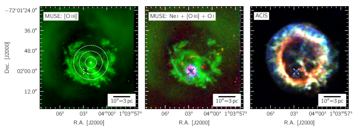
The existence of an X-ray point source in the middle of the low-ionization optical ring yields important clues regarding the exact nature of this structure. We identified this X-ray point source after reprocessing 322.6 ks of Chandra X-ray Observatory (CXO) observations of E 0102 (see Fig. 1). With an X-ray flux of (0.5–7.0 keV)= erg cm-2 s-1 (see the Methods for details), the X-ray point source is located at the position:
| R.A: 01h04m02.7s — Dec: -72∘02′00.2′′ [J2000]. |
The estimated absolute uncertainty of this position is 1.2′′, stemming both from the accuracy of the World Coordinate System (WCS) solution of the combined CXO observations, and the complex X-ray background of E 0102. One can expect 70 background X-ray sources (e.g. AGNs) with (0.5–2.0 keV) erg cm-2 s-1 per degree square (Gilli et al., 2007). Given that the area of the elliptical structure seen by MUSE is 15 square arcseconds, the probability of this X-ray source to lie in the background (i.e. a chance alignment) is extremely low, with only similar (or brighter) sources expected for this area. The spatial coincidence of the optical ring and the X-ray point source is thus a strong indication that the X-ray point source is located in the SMC, and directly associated with the elliptical structure itself.
An earlier, dedicated search for a compact object in E 0102 (Rutkowski et al., 2010) already located the same X-ray point source described above. For consistency, we shall thus refer to this X-ray source with the same name used by the earlier search: “p1”222Although Rutkowski et al. (2010) never explicitly quote the coordinates of p1, its location is made clear from their Fig. 1. This source was then merely listed as one candidate among seven sources within E 0102, but with no explicit comment. We hypothesize that source p1 may have (then) escaped a definitive identification because of its embedment in the diffuse and confusing X-ray background in the interior of E 0102, and/or because it was located outside of the “test source region”333The “test source region” was defined as the angular area where a compact object displaced by a natal kick would be most likely to be found. However, this area was computed using only a mean pulsar kick velocity. It was also less conservative than it could have been if the measurement errors associated with the explosion center had been included. defined by Rutkowski et al. (2010). Today, it is the unique capabilities of MUSE (i.e. its high sensitivity, fine spatial sampling and R3000 spectral resolution) that make it possible to spatio-kinematically isolate a distinctive optical ring of ejecta material centered on the X-ray source, thereby allowing us to firmly associate p1 with the SNR.
Evidently, the existence of an X-ray point source physically associated with E 0102 raises the question: could p1 be the as-of-yet unidentified compact object leftover by the supernova? In the other O-rich SNRs, compact objects come in two distinct types: (a) pulsars with active pulsar wind nebulae, as detected in G292.0+1.8 (Camilo et al., 2002; Park et al., 2007) and 0540-69.3 (Seward et al., 1984; Middleditch & Pennypacker, 1985; Mignani et al., 2010), and (b) Central Compact Objects (CCOs), as detected in Puppis A (Petre et al., 1996) and Cas A (Chakrabarty et al., 2001; Mereghetti et al., 2002). CCOs lack evidence of a pulsar wind nebula. They are detected only via their blackbody radiation, and are understood to be isolated, cooling neutron stars with thermal X-ray luminosities erg s-1 (Viganò et al., 2013). Extensive optical searches have failed to find any counterparts to the CCOs in Cas A and Puppis A, setting strong constraints on the possible accretion rate of material from the immediate surroundings of these objects (Wang et al., 2007; Mignani et al., 2009).
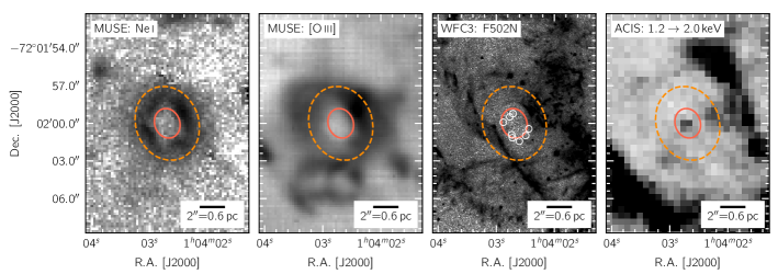
We searched for an optical counterpart to p1 in archival images from the Wide-Field Camera 3 (WFC3) and Advanced Camera for Survey (ACS) on the Hubble Space Telescope (HST). We found no suitable candidate down to an apparent magnitude upper limit of (see the Methods for details). For completeness, what is then the probability that the source p1 is a chance encounter of an X-ray source within the SMC itself? The SMC is host to a large number of High-Mass X-ray Binaries (HMXB), due in part to its star forming history. After a background AGN, this is statistically the most likely X-ray source one could encounter in the SMC (Sturm et al., 2013). However, the archival HST observations of the area rule out the presence of a high mass stellar counterpart (Haberl & Sturm, 2016) and thus the HMXB scenario. The lack of an optical counterpart also rules out a chance alignment with an X-ray-bright foreground star. The source p1 is visible above 1 keV, so that it is evidently not a Super-Soft X-ray Source: a class of X-ray sources that includes cataclysmic variables, planetary nebulae and accreting white dwarfs. The source p1 is also incompatible with isolated white dwarfs, which have soft X-ray spectra well fit by blackbody models with on the order of eV rather than keV (as is the case of p1, to be demonstrated shortly). The last remaining candidate for a chance alignment is that of a quiescent low-mass X-ray binary (LMXBs). To date, there is no known LMXB in the SMC, the number of which scales as a function of mass in a given galaxy (Gilfanov, 2004). We expect a maximum of 35 LMXBs in the SMC, leading to an LMXB density –and thus the probability of a chance alignment– of over the area of the optical ring. We are thus left with the only plausible scenario: that of p1 being the compact object of E 0102.
The low counts associated with the CXO observations of the source p1 hinder our ability to perform a detailed direct spectral analysis. Instead, we perform a “goodness of fit” analysis for a series of a) absorbed, single blackbody models and b) absorbed power-laws (see the Methods for details). In the first case, we find that the source p1 can be best represented by single blackbody model with keV. In the second case, we find that p1 is best represented by a power law with a photon index . Pulsars and pulsar wind nebulae can typically be described by power-laws with photon index (Kargaltsev & Pavlov, 2008): a range incompatible with the X-ray spectral energy distribution of the source p1, and thus indicating that p1 is most certainly not a pulsar. From our best-match single black-body model, we derive an intrinsic (unabsorbed) luminosity for the source p1 of (1.2–2.0 keV) erg s-1 and a (blackbody equivalent) source radius of 8.7 km. Altogether, these observational characteristics (X-ray brightness and temperature, X-ray energy distribution consistent with a soft thermal-like spectrum, lack of an optical counterpart and pulsar wind nebula, and spatial location within a SNR) lead us to propose the X-ray source p1 as a new addition to the CCO family (Pavlov et al., 2004); the first identified extragalactic CCO.
For comparison purposes, we simulate how the CCO of Cas A, whose X-ray signature has been extensively modelled (Pavlov & Luna, 2009), would appear if it were located at the distance of the SMC (see the Methods for details). The corresponding spectrum is shown in the top panel of Fig. 2. Our best match single-blackbody model is shown in the bottom panel of the same Figure. The Cas A-like CCO spectrum is 0.2 keV hotter than that of the source p1, but the brightness of both remain comparable. We note that similarly to p1, fitting the Cas A CCO with a power law also leads to a large photon index (Pavlov & Luna, 2009).
We now focus on the nature of the optical ring surrounding the newly identified CCO in E 0102. The elliptical structure has a semi-major axis of ′′ pc, an ellipticity , and a ring-width of ′′ pc (see Fig. 3). We find evidence of (at least) four intensity discontinuities along the ring to the N, S, E and S-W (see Fig. 4). Unambiguously identifying sub-structures within the ring itself will require sharper follow-up observations. In the HST WFC3 F502N image presented in Fig. 3, we note that a thin elliptical arc is present near the inner edge of the area coincident with the optical ring seen by MUSE, with a semi-major axis of ′′ pc. Given the spectral transmission window of the F502N filter, this arc is most certainly detected via its [O III] 4959,5007 emission. However, unambiguously separating it from the complex structure of the O-rich fast ejecta in this area is not straightforward. Our MUSE observations suggest that the high-ionization ring seen in [O III] 4959,5007 may be connected to a larger, funnel-like structure of shocked ejecta oriented along the line of sight.
![[Uncaptioned image]](/html/1803.01006/assets/x2.png)
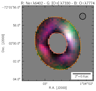
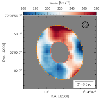
We performed a full spectral fit of the low-ionization optical ring (on a spaxel-by-spaxel basis, see the Methods for details), and derived its line-of-sight (LOS) kinematics (presented in Fig. 4). We find a clear asymmetry of km s-1 for the gas LOS velocity, broadly aligned with the ring’s major axis rotated by East-of-North. The radius of the low-ionization ring defined relative to the CCO implies an escape velocity of km s-1: given its LOS velocity, the ring material is thus not gravitationally bound to the CCO. Despite an evident blueshifted trough to the West (possibly due to intervening fast ejecta in the line of sight biasing the measurements of the line kinematics), the overall pattern is suggestive of an expanding torus, tilted with respect to the plane-of-the-sky, by , with an absolute expansion velocity of km s-1. If the torus has been expanding ballistically, this would imply an age of yr for the structure. This age is somewhat older than (though not incompatible with) the supernova age derived from the proper motion of the O-bright fast ejecta (Finkelstein et al., 2006), given the associated uncertainties. We discourage any over-interpretation of the arcsec-scale structures of the ring velocity map, recalling both the limited spatial resolution of the observations, and the existence of typical kinematic fitting artefacts associated with MUSE datacubes (Weilbacher et al., 2015; Vogt, 2015).
The exact physical mechanism(s) responsible for the excitation of the low-ionization ring remains uncertain. A spectrum dominated by recombination lines of Ne I and O I is not a proof that the ring is solely composed of Ne and O, but it does indicate that its electron temperature is 3000 K. Altogether, the optical spectrum and kinematics of the ring are consistent with dense, photoionized material which has not yet passed through the reverse shock. Quantifying the respective influence of photoionization by the CCO and/or by the overlying reverse shocked ejecta (for example, as modelled for SN 1006; Hamilton & Fesen, 1988) will require theoretical modelling beyond the scope of this Letter.
The existence of a slowly expanding torus of low-ionization material surrounding the CCO of E 0102 leads us to propose this location as the actual supernova explosion site of the system. If ejected during the supernova explosion, the slowly expanding material in the torus (in sharp contrast with the large velocities measured elsewhere in E 0102) would have originated from close to the supernova mass cut: the surface separating ejected material from material that forms the CCO (Umeda & Yoshida, 2016; Hix & Harris, 2016). But we also note that our current kinematic measurements do not rule out the possibility that this structure could pre-date the supernova explosion by a few kyr. Either way, given that the CCO is still located within 1.2′′ from center of the optical ring 2050 yr after the supernova explosion, we can set an upper-limit on the transverse velocity of the CCO of 170 km s-1. In this scenario, our newly defined explosion center would be located 5.9′′(1.77 pc) from the explosion center derived from the fast ejecta proper motion (Fig.1 and Finkelstein et al., 2006) – well within the 2-=6.8′′) uncertainty associated with that measurement. Setting the explosion site of E 0102 at the current location of the CCO would however imply a large offset with respect to the rather regular outer envelope of the X-ray emission of this SNR, requiring a specific set of circumstances to shape the expansion of the forward shock wave into such a regular structure. For example, the forward shock may be expanding inside a cavity carved by pre-supernova winds, which combined with a density gradient in the surrounding interstellar medium could induce an offset between the center of the X-ray shell and the explosion site.
In the alternative scenario, the supernova explosion occurred elsewhere, away from the current location of the CCO. Under these circumstances, we may be observing a CCO with high transverse velocity -e.g. 850 km s-1 in the plane-of-the-sky assuming the explosion center from Finkelstein et al. (2006)- as it catches up and collides (possibly) with surrounding ejecta. But given the timescales involved, we fail, at this point in time, to identify a physical mechanism able to account for the dimensions and kinematics of the low-ionization ring under these circumstances. A re-analysis of existing archival HST observations of E 0102 spanning 8 yr should help refine the measurement of the explosion center from the kinematics of the fast ejecta in E 0102. If precise enough, such a refined measurement can provide a strong test of our presently favored scenario: that of the supernova explosion originating at the current location of the CCO. At the same time, follow-up observations of the ring surrounding the CCO, with higher spatial resolution, are warranted to resolve the sub-structures within the ring, link the low-ionization material to the elliptical [O III] arc detected in HST images of the area, and refine the derivation of its kinematic signature and age. The Adaptive Optics modes of MUSE appear particularly suited to the task.
Online Content
Methods, along with additional Supplementary Information display items, are available in the online version of the paper; references unique to these sections appear only in the online paper.
References
- Astropy Collaboration et al. (2013) Astropy Collaboration, Robitaille, T. P., Tollerud, E. J., et al. 2013, Astron. Astrophys., 558, A33
- Bacon et al. (2010) Bacon, R., Accardo, M., Adjali, L., et al. 2010, in Proc. SPIE, Vol. 7735, Ground-Based and Airborne Instrumentation for Astronomy III, 773508
- Blair et al. (2000) Blair, W. P., Morse, J. A., Raymond, J. C., et al. 2000, Astrophys. J., 537, 667
- Bonnarel et al. (2000) Bonnarel, F., Fernique, P., Bienaymé, O., et al. 2000, Astron. Astrophys.Supplement Series, 143, 33
- Camilo et al. (2002) Camilo, F., Manchester, R. N., Gaensler, B. M., Lorimer, D. R., & Sarkissian, J. 2002, The Astrophys. J. Letters, 567, L71
- Chakrabarty et al. (2001) Chakrabarty, D., Pivovaroff, M. J., Hernquist, L. E., Heyl, J. S., & Narayan, R. 2001, Astrophys. J., 548, 800
- Cleveland (1979) Cleveland, W. S. 1979, Journal of the American Statistical Association, 74, 829
- Dickey & Lockman (1990) Dickey, J. M. & Lockman, F. J. 1990, Annu. Rev. Astron. Astr., 28, 215
- Dopita et al. (1981) Dopita, M. A., Tuohy, I. R., & Mathewson, D. S. 1981, The Astrophys. J. Letters, 248, L105
- Finkelstein et al. (2006) Finkelstein, S. L., Morse, J. A., Green, J. C., et al. 2006, Astrophys. J., 641, 919
- Gaia Collaboration et al. (2016a) Gaia Collaboration, Brown, A. G. A., Vallenari, A., et al. 2016a, Astron. Astrophys., 595, A2
- Gaia Collaboration et al. (2016b) Gaia Collaboration, Prusti, T., de Bruijne, J. H. J., et al. 2016b, Astron. Astrophys., 595, A1
- Gilfanov (2004) Gilfanov, M. 2004, Mon. Not. R. Astron. Soc., 349, 146
- Gilli et al. (2007) Gilli, R., Comastri, A., & Hasinger, G. 2007, Astron. Astrophys., 463, 79
- Graczyk et al. (2014) Graczyk, D., Pietrzyński, G., Thompson, I. B., et al. 2014, Astrophys. J., 780, 59
- Haberl & Sturm (2016) Haberl, F. & Sturm, R. 2016, Astron. Astrophys., 586, A81
- Hamilton & Fesen (1988) Hamilton, A. J. S. & Fesen, R. A. 1988, Astrophys. J., 327, 178
- Helou et al. (1991) Helou, G., Madore, B. F., Schmitz, M., et al. 1991, Databases and On-line Data in Astronomy, 171, 89
- Hix & Harris (2016) Hix, W. R. & Harris, J. A. 2016, in Handbook of Supernovae, ed. A. W. Alsabti & P. Murdin (Springer International Publishing), 1–19
- Hunter (2007) Hunter, J. D. 2007, Computing in Science and Engineering, 9, 90
- Joye & Mandel (2003) Joye, W. A. & Mandel, E. 2003, in Astronomical Data Analysis Software and Systems XII ASP Conference Series, Vol. 295, 489
- Kargaltsev & Pavlov (2008) Kargaltsev, O. & Pavlov, G. G. 2008, in , eprint: arXiv:0801.2602, 171–185
- Kramida et al. (2016) Kramida, A., Ralchenko, Y., Reader, J., & Team, N. A. 2016, NIST Atomic Spectra Database (Ver. 5.4)
- Mereghetti et al. (2002) Mereghetti, S., Tiengo, A., & Israel, G. L. 2002, Astrophys. J., 569, 275
- Middleditch & Pennypacker (1985) Middleditch, J. & Pennypacker, C. 1985, Nature, 313, 659
- Mignani et al. (2009) Mignani, R. P., de Luca, A., Mereghetti, S., & Caraveo, P. A. 2009, Astron. Astrophys., 500, 1211
- Mignani et al. (2010) Mignani, R. P., Sartori, A., de Luca, A., et al. 2010, Astron. Astrophys., 515, A110
- Moré (1978) Moré, J. J. 1978, in Numerical Analysis: Proceedings of the Biennial Conference Held at Dundee, June 28–July 1, 1977 (Springer Berlin Heidelberg), 105–116
- Park et al. (2007) Park, S., Hughes, J. P., Slane, P. O., et al. 2007, The Astrophys. J. Letters, 670, L121
- Pavlov & Luna (2009) Pavlov, G. G. & Luna, G. J. M. 2009, Astrophys. J., 703, 910
- Pavlov et al. (2004) Pavlov, G. G., Sanwal, D., & Teter, M. A. 2004, in IAU Symposium, ed. F. Camilo & B. M. Gaensler, Vol. 218, eprint: arXiv:astro-ph/0311526, 239
- Petre et al. (1996) Petre, R., Becker, C. M., & Winkler, P. F. 1996, The Astrophys. J. Letters, 465, L43
- Plucinsky et al. (2017) Plucinsky, P. P., Beardmore, A. P., Foster, A., et al. 2017, Astron. Astrophys., 597, A35
- Robitaille & Bressert (2012) Robitaille, T. & Bressert, E. 2012, Astrophysics Source Code Library, ascl:1208.017
- Rutkowski et al. (2010) Rutkowski, M. J., Schlegel, E. M., Keohane, J. W., & Windhorst, R. A. 2010, Astrophys. J., 715, 908
- Sasaki et al. (2006) Sasaki, M., Gaetz, T. J., Blair, W. P., et al. 2006, Astrophys. J., 642, 260
- Scowcroft et al. (2016) Scowcroft, V., Freedman, W. L., Madore, B. F., et al. 2016, Astrophys. J., 816, 49
- Seabold & Perktold (2010) Seabold, S. & Perktold, J. 2010, in Proc. of the 9th Python in Science Conference, 57–61
- Seitenzahl et al. (2018) Seitenzahl, I. R., Vogt, F. P. A., Terry, J. P., et al. 2018, The Astrophys. J. Letters, 853, L32
- Seward et al. (1984) Seward, F. D., Harnden, Jr., F. R., & Helfand, D. J. 1984, The Astrophys. J. Letters, 287, L19
- Seward & Mitchell (1981) Seward, F. D. & Mitchell, M. 1981, Astrophys. J., 243, 736
- Sturm et al. (2013) Sturm, R., Haberl, F., Pietsch, W., et al. 2013, Astron. Astrophys., 558, A3
- Sutherland & Dopita (1995) Sutherland, R. S. & Dopita, M. A. 1995, Astrophys. J., 439, 381
- Tananbaum (1999) Tananbaum, H. 1999, International Astronomical Union Circular, 7246, 1
- Umeda et al. (2000) Umeda, H., Nomoto, K., Tsuruta, S., & Mineshige, S. 2000, The Astrophys. J. Letters, 534, L193
- Umeda & Yoshida (2016) Umeda, H. & Yoshida, T. 2016, in Handbook of Supernovae, ed. A. W. Alsabti & P. Murdin (Springer International Publishing), 1–18
- van den Bergh (1988) van den Bergh, S. 1988, Astrophys. J., 327, 156
- Viganò et al. (2013) Viganò, D., Rea, N., Pons, J. A., et al. 2013, Mon. Not. R. Astron. Soc., 434, 123
- Vogt (2015) Vogt, F. P. A. 2015, PhD Thesis, Australian National University
- Vogt et al. (2017) Vogt, F. P. A., Seitenzahl, I. R., Dopita, M. A., & Ghavamian, P. 2017, Astron. Astrophys., 602, L4
- Wang et al. (2007) Wang, Z., Kaplan, D. L., & Chakrabarty, D. 2007, Astrophys. J., 655, 261
- Weilbacher et al. (2015) Weilbacher, P. M., Monreal-Ibero, A., Kollatschny, W., et al. 2015, Astron. Astrophys., 582, A114
- Winkler & Kirshner (1985) Winkler, P. F. & Kirshner, R. P. 1985, Astrophys. J., 299, 981
Acknowledgments
We thank Eric M. Schlegel and the other two (anonymous) reviewers for their constructive comments. This research has made use of brutus, a Python module to process data cubes from integral field spectrographs hosted at
http://fpavogt.github.io/brutus/. For this analysis, brutus relied on statsmodel (Seabold & Perktold, 2010), matplotlib (Hunter, 2007), astropy, a community-developed core Python package for Astronomy
(Astropy Collaboration et al., 2013), aplpy, an open-source plotting package for Python (Robitaille & Bressert, 2012), and montage, funded by the National Science Foundation under Grant Number ACI-1440620 and previously funded by the National Aeronautics and Space Administration’s Earth Science Technology Office, Computation Technologies Project, under Cooperative Agreement Number NCC5-626 between NASA and the California Institute of Technology.
This research has also made use of drizzlepac, a product of the Space Telescope Science Institute, which is operated by AURA for NASA, of the aladin interactive sky atlas (Bonnarel et al., 2000), of saoimage ds9 (Joye & Mandel, 2003) developed by Smithsonian Astrophysical Observatory, of NASA’s Astrophysics Data System, and of the NASA/IPAC Extragalactic Database (Helou et al., 1991) which is operated by the Jet Propulsion Laboratory, California Institute of Technology, under contract with the National Aeronautics and Space Administration.
This work has made use of data from the European Space Agency (ESA) mission Gaia
(https://www.cosmos.esa.int/gaia), processed by the Gaia Data Processing and Analysis Consortium (DPAC,
https://www.cosmos.esa.int/web/gaia/dpac/consortium). Funding for the DPAC has been provided by national institutions, in particular the institutions participating in the Gaia Multilateral Agreement. Some of the data presented in this paper were obtained from the Mikulski Archive for Space Telescopes (MAST). STScI is operated by the Association of Universities for Research in Astronomy, Inc., under NASA contract NAS5-26555. Support for MAST for non-HST data is provided by the NASA Office of Space Science via grant NNX09AF08G and by other grants and contracts.
IRS was supported by Australian Research Council Grant FT160100028. PG acknowledges support from HST grant HST-GO-14359.011. AJR has been funded by the Australian Research Council grant numbers CE110001020 (CAASTRO) and FT170100243. FPAV and IRS thank the CAASTRO AI travel grant for generous support. PG thanks the Stromlo Distinguished Visitor Program.
Based on observations made with ESO Telescopes at the La Silla Paranal Observatory under program ID 297.D-5058.
Author Contributions
F.P.A.V. reduced and lead the analysis of the MUSE datacube. E.S.B. lead the spectral analysis of the Chandra dataset. All authors contributed to the interpretation of the observations, and the writing of the manuscript.
Author Information
The authors declare no competing financial interests. Readers are welcome to comment on the online version of the paper. Correspondence and requests for materials should be addressed to F.P.A.V. (frederic.vogt@alumni.anu.edu.au).
Methods
Observations, data reduction &
post-processing
MUSE
The MUSE observations of E 0102 acquired under Director Discretionary Time program 297.D-5058 (P.I.: Vogt) are comprised of nine 900 s exposures on-source. The detailed observing strategy and data reduction procedures are described exhaustively in Vogt et al. (2017), to which we refer the interested reader for details. Similarly to that work, the combined MUSE cube discussed in the present report was continuum-subtracted using the Locally Weighted Scatterplot Smoothing algorithm (Cleveland, 1979). This non-parametric approach is particularly suitable to reliably remove both the stellar and nebular continuum in all spaxels of the datacube without the need for manual interaction.
The one major difference between the MUSE datacube of E 0102 described in Vogt et al. (2017) and this work lies in the World Coordinate System (WCS) solution. For this analysis, we have refined the WCS solution (then derived by comparing the MUSE white-light image with the Digitized Sky Survey 2 red image of the area) by anchoring it to the Gaia (Gaia Collaboration et al., 2016b) Data Release 1 (DR1 Gaia Collaboration et al., 2016a) entries of the area. In doing so, we estimate our absolute WCS accuracy to be of the order of 0.2′′.
CXO
E 0102 has been used as an X-ray calibration source for many years (Plucinsky et al., 2017), so that there exist numerous CXO observations of this system in the archive. When selecting datasets to assemble a deep X-ray view of E 0102, we applied the following, minimal selection criteria:
-
•
datamode = vfaint
-
•
no CC-mode observations
-
•
-
•
sepn 1.2 arcmin, with the reference point set to R.A.:01h04m02s.4, Dec.:-72∘01′55′′.3 [J2000].
These criteria ensure that we combine a uniform set of observations with minimal instrumental background. The last condition ensures that we use the observations with the highest possible spatial resolution, by using only those pointings with E 0102 close from the optical axis of the telescope. The resulting list of 28 observations matching these criteria is presented in Table 1. We did not apply any selection criteria on the year or the depth of the observations: a direct consequence of setting the focus of our analysis on the characterization of the detected X-ray point source (for which we find no evidence of proper motion in the CXO observations), rather than on the fast-moving ejecta.
We fetched and reprocessed all these datasets using ciao 4.9 and caldb 4.7.3, via the chandra_repro routine. We searched for evidence of background flares by generating images in the 0.5-8.0 keV energy range while removing the bright sources in the field of view, including E 0102. Light curves were then created from the entire remaining image and inspected by eye. We dropped three observations (Obs. I.D.: 5123, 5124 and 6074) that show signs of flaring, prior to combining the remaining ones using the reproject_obs routine. All X-ray images of E 0102 presented in this work were extracted from this combined, reprojected dataset. We did not perform any adjustment to the existing WCS solution of the combined dataset, which given our target on-axis selection criteria can be expected to be of the order of 0.6′′.
| Obs. I.D. | Date | Depth | Signs of flaring ? |
|---|---|---|---|
| [ks] | |||
| 3519 | 2003-02-01 | 8.0 | |
| 3520 | 2003-02-01 | 7.6 | |
| 3545 | 2003-08-08 | 7.9 | |
| 3544 | 2003-08-10 | 7.9 | |
| 5123 | 2003-12-15 | 20.3 | yes |
| 5124 | 2003-12-15 | 7.9 | yes |
| 5131 | 2004-04-05 | 8.0 | |
| 5130 | 2004-04-09 | 19.4 | |
| 6075 | 2004-12-18 | 7.9 | |
| 6042 | 2005-04-12 | 18.9 | |
| 6043 | 2005-04-18 | 7.9 | |
| 6074 | 2004-12-16 | 19.8 | yes |
| 6758 | 2006-03-19 | 8.1 | |
| 6765 | 2006-03-19 | 7.6 | |
| 6759 | 2006-03-21 | 17.9 | |
| 6766 | 2006-06-06 | 19.7 | |
| 8365 | 2007-02-11 | 21.0 | |
| 9694 | 2008-02-07 | 19.2 | |
| 10654 | 2009-03-01 | 7.3 | |
| 10655 | 2009-03-01 | 6.8 | |
| 10656 | 2009-03-06 | 7.8 | |
| 11957 | 2009-12-30 | 18.4 | |
| 13093 | 2011-02-01 | 19.0 | |
| 14258 | 2012-01-12 | 19.0 | |
| 15467 | 2013-01-28 | 19.1 | |
| 16589 | 2014-03-27 | 9.6 | |
| 18418 | 2016-03-15 | 14.3 | |
| 19850 | 2017-03-19 | 14.3 |
HST
We downloaded from the Barbara A. Mikulski Archive for the Space Telescopes (MAST) all the observations of E 0102 acquired with the Advanced Camera for Survey (ACS) and the Wide Field Camera 3 (WFC3) that used narrow, medium and wide filters. These belong to three observing programs: 12001 (ACS, P.I.: Green), 12858 (ACS, P.I.: Madore) and 13378 (WFC3, P.I.: Milisavljevic). The exhaustive list of all the individual observations is presented in Table 2.
| Program I.D. | Observation I.D. | P.I. | Observation Date | Instrument | Filter | Exposure time |
|---|---|---|---|---|---|---|
| [s] | ||||||
| 13378 | ICBQ01010 | Milisavljevic | 2014-05-12 | WFC3/UVIS | F280N | 1650 |
| 13378 | ICBQ01020 | Milisavljevic | 2014-05-12 | WFC3/UVIS | F280N | 1100 |
| 13378 | ICBQ01050 | Milisavljevic | 2014-05-12 | WFC3/UVIS | F373N | 2268 |
| 13378 | ICBQ03070 | Milisavljevic | 2014-05-14 | WFC3/UVIS | F467M | 1362 |
| 12001 | J8R802010 | Green | 2003-10-15 | ACS/WFC | F475W | 1520 |
| 12001 | J8R802011 | Green | 2003-10-15 | ACS/WFC | F475W | 760 |
| 12858 | JBXR02010 | Madore | 2013-04-10 | ACS/WFC | F475W | 2044 |
| 13378 | ICBQ02010 | Milisavljevic | 2014-05-13 | WFC3/UVIS | F502N | 1653 |
| 13378 | ICBQ02020 | Milisavljevic | 2014-05-13 | WFC3/UVIS | F502N | 1100 |
| 12001 | J8R802020 | Green | 2003-10-15 | ACS/WFC | F550M | 1800 |
| 12001 | J8R802021 | Green | 2003-10-15 | ACS/WFC | F550M | 900 |
| 13378 | ICBQ03080 | Milisavljevic | 2014-05-14 | WFC3/UVIS | F645N | 1350 |
| 13378 | ICBQ03010 | Milisavljevic | 2014-05-14 | WFC3/UVIS | F657N | 1653 |
| 13378 | ICBQ03020 | Milisavljevic | 2014-05-14 | WFC3/UVIS | F657N | 1102 |
| 12001 | J8R802030 | Green | 2003-10-15 | ACS/WFC | F658N | 1440 |
| 12001 | J8R802031 | Green | 2003-10-15 | ACS/WFC | F658N | 720 |
| 13378 | ICBQ03030 | Milisavljevic | 2014-05-14 | WFC3/UVIS | F665N | 1719 |
| 13378 | ICBQ03040 | Milisavljevic | 2014-05-14 | WFC3/UVIS | F665N | 1146 |
| 13378 | ICBQ03050 | Milisavljevic | 2014-05-14 | WFC3/UVIS | F673N | 1719 |
| 13378 | ICBQ03060 | Milisavljevic | 2014-05-14 | WFC3/UVIS | F673N | 1146 |
| 12001 | J8R802050 | Green | 2003-10-15 | ACS/WFC | F775W | 1440 |
| 12001 | J8R802051 | Green | 2003-10-15 | ACS/WFC | F775W | 720 |
| 12001 | J8R802040 | Green | 2003-10-15 | ACS/WFC | F850LP | 1440 |
| 12001 | J8R802041 | Green | 2003-10-15 | ACS/WFC | F850LP | 720 |
All the calibrated, CTE-corrected, individual exposures (*_flc.fits) obtained from MAST were fed to the tweakreg routine to correct their WCS solutions. We used a custom python script relying on the drizzlepac 2.1.13, astroquery and astropy packages to do so automatically for all the filters. We used the Gaia (Gaia Collaboration et al., 2016b) DR1(Gaia Collaboration et al., 2016a) catalogue as the reference set of point source coordinates and fluxes. Using the same script, we subsequently fed all the images for a given filter to the astrodrizzle routine, and combined them into a single final frame. We set the pixel scale to 0.04′′ for all filters for simplicity, but note that this value does not affect significantly our conclusions. We also note that combining observations separated by several years is not ideal from the perspective of the fast ejecta (whose proper motion imply a blurring of the final image). It is however a suitable approach in the present case, i.e. in order to look for an optical counterpart to the X-ray point source detected with CXO, provided that its proper motion is smaller than 0.08/10=0.008′′ yr-12350 km s-1.
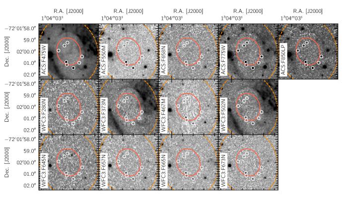
Postage stamp images of the optical ring area detected with MUSE, for all re-processed HST camera+filter combinations, are presented in Fig. 5. We find no evidence for an optical counterpart to the X-ray point source detected with CXO. Four point sources are detected within the central gap of the low-ionization optical ring detected with MUSE, but we rule them out as suitable candidate based on their largely off-center locations. E 0102 was not observed by HST down to the same depth in each filter. The strongest constraints for the brightness of a possible optical counterpart come from the ACS F475W image (4324 s on-source), the ACS F775W image (2160 s on-source), and the ACS F850LP (2160 s on-source). Specifically, we derive an upper limit for the magnitude of a possible optical counterpart to the X-ray source of m, m and m, noting that the F475W image is severely affected by contaminating [O III] 4959,5007 emission from the fast ejecta, falling within the filter bandpass.
CXO characterization of the CCO in E 0102
Spatial characterization
Combined X-ray images of E 0102 were created in the standard CXO ACIS source detection energy bands, as well as the ultrasoft band (0.2–0.5 keV), using the ciao script merge_obs. We ran the Mexican-Hat wavelet source detection tool wavdetect on all the combined images, which confirmed the presence of the point source p1 already detected by Rutkowski et al. (2010), and coincident with the low-ionization optical ring discovered with MUSE. As we are exclusively searching for a point source embedded in the diffuse emission of the hot ejecta from the SNR, the source detection algorithm was run with no point spread function (PSF) map on “fine” scales (the wavdetect scales parameter was set to “1 2”). The derived spatial parameters for each band are summarized in Table 3.
| Band | Energy | R.A. | Dec. | Semi-major axis | Semi-minor axis | Pos. Angle | Detection significance |
|---|---|---|---|---|---|---|---|
| [keV] | [J2000] | [J2000] | [arcsec] | [arcsec] | [deg] | ||
| Broad | 0.5–7.0 | 01:04:02.73 | -72:02:00.36 | 1.6 | 1.1 | 50.9 | 8.60 |
| Ultrasoft | 0.2–0.5 | 01:04:02.73 | -72:02:00.23 | 1.2 | 1.0 | 58.5 | 2.10 |
| Soft | 0.5–1.2 | 01:04:02.77 | -72:02:00.66 | 1.9 | 0.9 | 74.2 | 5.78 |
| Medium | 1.2–2.0 | 01:04:02.75 | -72:02:00.14 | 1.2 | 1.0 | 54.0 | 8.30 |
| Hard | 2.0–7.0 | 01:04:02.75 | -72:02:00.19 | 2.2 | 1.8 | 91.8 | 5.45 |
Without a PSF map, wavdetect uses the smallest wavelet scale found to derive the source properties. This approach may lead to incorrect parameters at large off-axis angles, but our target on-axis selection criteria for the CXO datasets ensures that this will not have a very significant effect in the present case. The detection process itself is unaffected by the lack of inclusion of a PSF map. We did experiment with PSF maps weighted by both exposure time and exposure map for the combined broad band dataset. But in each instance, the algorithm detects the entire filamentary structure of E 0102, rather than a point source itself444For more details on running wavedetect on combined datasets, see http://cxc.harvard.edu/ciao/threads/wavdetect merged/index.html.
Spectral characterization
We manually extracted the counts of the source p1 in all bands using the region derived from the automated point source search in the medium CXO band, where it is most reliably detected by wavdetect (see Table 3). Background counts are derived from an annulus centered on the source, and with inner and outer radii of 1.2′′ and 1.8′′, respectively. The counts derived from each band are summarized in Table 4.
| Band | Energy | Counts(a) | Counts(b) | (c) | (d) | (e) |
|---|---|---|---|---|---|---|
| [keV] | [erg cm-2 s-1] | [erg cm-2 s-1] | [erg s-1] | |||
| Broad | 0.5–7.0 | 469 | 1.37 | |||
| Ultrasoft | 0.2–0.5 | (f) | 4 | 0.17 | (f) | |
| Soft | 0.5–1.2 | 279 | 1.11 | |||
| Medium | 1.2–2.0 | 172 | 0.28 | |||
| Hard | 2.0–7.0 | 7 | 0.02 |
-
(a)
Observed (background subtracted) counts for the source p1.
-
(b)
Simulated source counts for the best-fit, absorbed single blackbody model (, with keV).
-
(c)
The X-ray flux (in units of erg cm-2 s-1) of the best-fit, absorbed single blackbody model.
-
(d)
The observed X-ray flux (in units of erg cm-2 s-1) of the source p1, computed with the ECFs derived (for each energy band) from the best-fit, absorbed single blackbody model and associated simulated dataset.
-
(e)
Intrinsic (i.e. unabsorbed) X-ray luminosity implied from the assumed absorbed Blackbody model, assuming a distance of 62.1 kpc to the SMC and a 10% error on the exact distance to E 0102 within the SMC.
-
(f)
3 upper limit.
Our chosen parameters for the “background annulus” are motivated by the complex X-ray background emission throughout E 0102. This annulus is narrow enough to avoid brighter filamentary structures nearby, but large enough for a reliable estimate of the local background level close to and around the source. Whilst our region size is small, approximately 90% of the encircled energy still lies within 1′′ of the central pixel555See Figure 6.10 on
http://cxc.cfa.harvard.edu/proposer/POG/html/ACIS.html. Pavlov & Luna (2009) also adopt a similar region size (1.5′′ in radius) in their analysis of the Galactic CCO in Cas A. We note that we find no evidence for the background annuli to contain any knots or feature associated with the Ne and Mg metal lines, after the visual inspection of dedicated channel maps centered at 0.8496 keV and 1.2536 keV, each 130 eV wide.
The low counts associated with source p1 hinder our ability to extract robust parameters from a direct spectral fitting. Instead, for comparison purposes, we first investigate how the CCO of Cas A would appear to an observer if it were located at the distance of the SMC, with an absorbing column equal to that of E 0102. We simulate the double-blackbody model of Pavlov & Luna (2009) to do so, using xspec v.12.9.0 and the fakeit command. These authors fit absorbed blackbody, power law and neutron star atmosphere models to a single 70.2 ks CXO observation of Cas A, with a count rate of 0.1 counts s-1. They find that the X-ray spectrum of the CCO of Cas A is equally well described by both an absorbed double neutron star model (represented as in xspec) and an absorbed double blackbody model (represented as in xspec). We voluntarily reproduce only the double blackbody model here, as the double neutron star model has many more parameters which are not explicitly described.
We include two absorption terms to the model: one to account for the Galactic absorption (set to ; Dickey & Lockman, 1990), and another set to the intrinsic absorption in the south-east region of E 0102, where the source p1 is located (; Sasaki et al., 2006). The spectrum is then normalised to have the same unabsorbed luminosity as that reported by Pavlov & Luna (2009), over the same energy range. In summary, our final model is represented by in xspec, where is a constant. We simulate the spectrum of such a source using the CXO cycle 19 canned response matrices666Available at http://cxc.harvard.edu/caldb/prop_plan/imaging/index.html and an exposure time of 323 ks, matching the total depth of our combined CXO observations.
We compare the simulated spectrum of Cas A with the measured counts of the source p1 (in each of the narrow energy bands) in the top panel of Fig. 2: p1 appears cooler than would a Cas A-like CCO at the same location. This is not necessarily surprising, given that E 0102 is 1700 yr older than Cas A.
Next, to derive X-ray fluxes and luminosities for the source p1 in E 0102, we use xspec’s fakeit with the cycle 19 canned response matrices to simulate a) absorbed single blackbody models and b) absorbed power laws in the same manner as above. These models are represented by and in xspec. We restrict ourselves to single blackbody and power law models, as the counts associated with the source p1 are insufficient to reliably constraint more complex ones, including double blackbody models. The Galactic and intrinsic absorption components are once again set to and , respectively. We generate spectra with temperatures ranging from 0.10–0.49 keV in steps of 0.01 keV for the blackbody models, and with a photon index ranging from 0.50–5.25 in steps of 0.25 for the power law models. Each spectrum is normalised so that the total number of counts over 0.5–7.0 keV (i.e. the broad band) in a 323 ks exposure is consistent with that of the source p1 detected in our merged data set of E 0102. All our models are compared with the measured counts of the source p1 in Fig. 6 to 8.
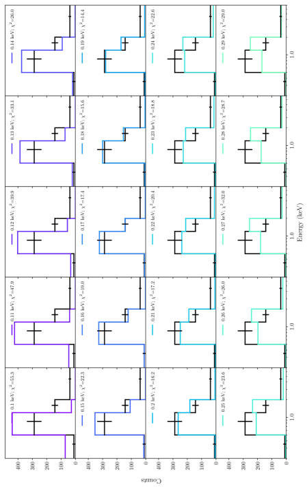
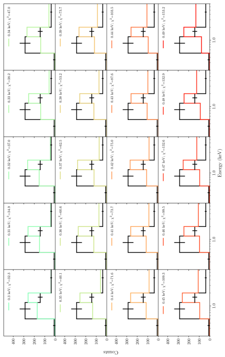
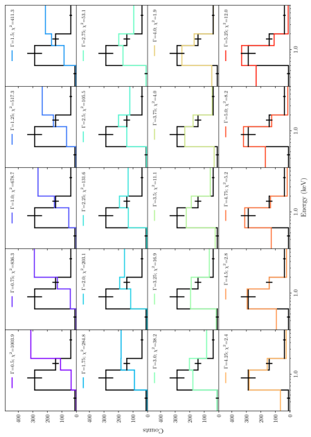
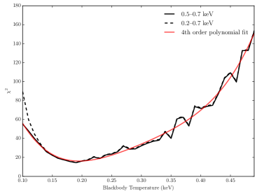
We calculate the of each of the single blackbody models with respect to the data over both the 0.5–7.0 keV and 0.2–7.0 keV energy ranges, and for each of the power law models with respect to the data over the 0.5–7.0 keV energy range. We exclude the ultrasoft band from some of these ranges, as the CXO response files are less accurate below 0.5 keV777see http://cxc.harvard.edu/caldb/prop_plan/imaging/index.html. We show in Fig. 9 the distribution of these values as a function of the blackbody temperature of the models, together with the fourth order polynomial best fit to the 0.5–0.7 keV data. For the absorbed, single blackbody models, we find that the source p1 is best characterised by a blackbody with keV. For the absorbed, power law models, we find that the source p1 is best characterised by models with a photon index .
Fitting a single blackbody model to Cas A (with a derived a temperature of 0.4 keV) underestimates the CCO flux at higher energies (Pavlov & Luna, 2009). The same can be seen in our simulations: our best-match, absorbed single blackbody model underestimate the number counts of the source p1 in the hard CXO band. The flux values associated with the best-fit keV model are included in Table 4 along with the implied intrinsic (i.e. un-absorbed) X-ray luminosity. The errors associated with the latter stem from an assumed 10% uncertainty in the depth of E 0102 within the SMC. In the same Table, we also present the observed X-ray flux of the source p1, computed from the observed data using the energy conversion factors (ECFs) derived (for each energy band) from the best-fit, absorbed single blackbody model with keV.
We note that our derived fluxes and luminosities are subject to caveats. First, our simulated spectra assume that we have a single 323 ks observation performed in cycle 19 of CXO’s lifetime, rather than several observations spanning over a decade. Second, the background subtraction and determination for the point source p1 is non-trival, as it is embedded in bright, spatially complex background emission. A more complex spectroscopic analysis of this X-ray point source, outside the scope of this report, ought to address these points carefully.
MUSE spectral characterization of the optical ring
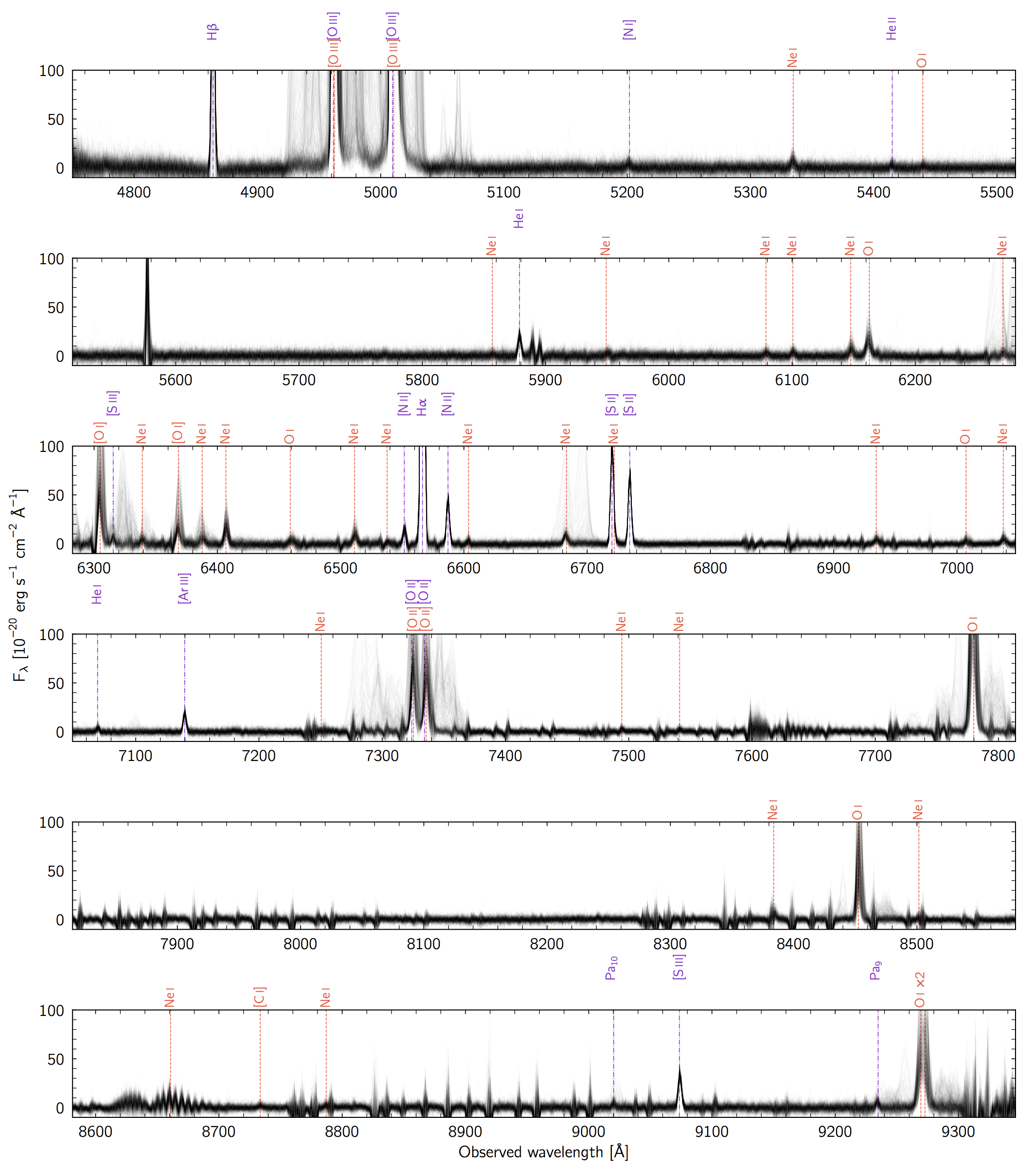
We performed a full fit of the MUSE spectra associated with each of the 492 spaxels contained within the area of the optical ring. The fitted spaxels are located within two ellipses with semi-major axis of 1.2′′ and 3.0′′ centered on the CCO (R.A: 01h04m02.7s — Dec: -72∘02′00.2′′ [J2000]), and rotated by 20∘ East-of-North. The ring is detected in 35 lines of Ne I, O I, [O I], and [C I], all of which were identified following a manual, visual inspection of every spectral channel in the continuum-subtracted MUSE datacube (see Fig. 10). An intensity increase spatially coincident with the ring is also detected in 4 lines of [O III] and [O II], but the surrounding emission of these lines is spatially more extended in comparison to the lower-ionization lines, as illustrated in Fig. 3. The low- and high-ionization lines thus likely originate from physically distinct volumes.
The line fitting is performed using a custom routine relying on the python implementation of mpfit, a script that uses the Levenberg-Marquardt technique (Moré, 1978) to solve least-squares problems, based on an original Fortran code part of the minpack-1 package. We do not include the [O III] 4959,5007 lines in the fitting: their large intensity with respect to the lower-ionization emission lines and the presence of several fast ejecta knots throughout the footprint of the ring affect the derived kinematic signature of the ring. We do however include the [O II] 7320,7330 lines in the list of fitted lines for comparison purposes, after having ensured that their inclusion does not affect the outcome of the spectral fit at a significant level. Finally, we do not include the Ne I 6266, Ne I 6334, Ne I 6383, Ne I 6678, Ne I 6717, and Ne I 8654 emission lines in the fit, as these lines are strongly contaminated by residual sky lines, bright emission lines from fast ejecta along specific lines-of-sight, and/or background H II-like emission.
For each of the 492 spaxels within the footprint of the ring, the selected 31 emission lines are fitted simultaneously, each with a single Gaussian component tied to a common, observed LOS velocity . The velocity dispersion for a specific line wavelength is set to:
| (1) |
with km s-1 the assumed-constant underlying gas velocity dispersion, and the wavelength-dependant instrumental spectral dispersion of MUSE. The ring emission lines are spectrally unresolved by MUSE. Here we fix their underlying velocity dispersion to ensure a robust fit for all spaxels, including those towards the inner and outer edges of the ring with lower S/N, noting that the fitting results are not significantly affected by the exact value of . Dedicated observations with higher spectral resolution are required to constrain this parameter.
The measured line fluxes for all fitted lines are presented in Table 5. The rest frame line wavelengths were obtained from the NIST Atomic Spectra Database (Kramida et al., 2016). The LOS velocity map of the ring is shown in Fig. 4, together with a pseudo-RGB image of the fitted area in the light of Ne I 6402, [O II] 7330, and O I 7774. The mean fitted ring spectrum is compared to the observed spectra in Fig. 10. The mean velocity of the optical ring is km s-1 with respect to the background H II-like emission of the SMC. The uncertainty is dominated by the somewhat irregular appearance of the velocity map: the error associated with the fitting alone is of the order of 5 km s-1.
| Line | ||||
| [Å] | [ erg s-1 cm-2] | [ erg s-1 cm-2 arcsec-2] | [ erg s-1 cm-2 arcsec-2] | |
| [O III] | 4958.911 | N/A | N/A | N/A |
| [O III] | 5006.843 | N/A | N/A | N/A |
| Ne I | 5330.7775 | 460.4 | ||
| O I | 5435.78 | 236.4 | ||
| Ne I | 5852.4878 | 213.6 | ||
| Ne I | 5944.8340 | 249.3 | ||
| Ne I | 6074.3376 | 263.6 | ||
| Ne I | 6096.1630 | 286.9 | ||
| Ne I | 6143.0627 | 546.8 | ||
| O I | 6158.18 | 886.9 | ||
| Ne I | 6266.4952 | N/A | N/A | N/A |
| O I | 6300.304 | 5858.3 | ||
| Ne I | 6334.4276 | N/A | N/A | N/A |
| O I | 6363.776 | 1943.9 | ||
| Ne I | 6382.9914 | N/A | N/A | N/A |
| Ne I | 6402.248 | 736.4 | ||
| O I | 6454.44 | 303.4 | ||
| Ne I | 6506.5277 | 561.7 | ||
| Ne I | 6532.8824 | 170.8 | ||
| Ne I | 6598.9528 | 184.2 | ||
| Ne I | 6678.2766 | N/A | N/A | N/A |
| Ne I | 6717.0430 | N/A | N/A | N/A |
| Ne I | 6929.4672 | 289.4 | ||
| O I | 7002.23 | 301.6 | ||
| Ne I | 7032.4128 | 303.8 | ||
| Ne I | 7245.1665 | 189.7 | ||
| [O II] | 7319.92 | 7512.0 | ||
| [O II] | 7330.19 | 5273.2 | ||
| Ne I | 7488.8712 | 181.5 | ||
| Ne I | 7535.7739 | 179.8 | ||
| O I | 7774.17 | 9614.1 | ||
| Ne I | 8377.6070 | 469.5 | ||
| O I | 8446.36 | 3949.6 | ||
| Ne I | 8495.3591 | 227.9 | ||
| Ne I | 8654.3828 | N/A | N/A | N/A |
| [C I] | 8727.13 | 211.1 | ||
| Ne I | 8780.6223 | 259.2 | ||
| O I | 9262.67 | 2758.9 | ||
| O I | 9266.01 | 3285.6 |
Data Availability Statement
The data that support the plots within this paper and other findings of this study are available from the corresponding author upon reasonable request. The MUSE observations are available from the ESO archive under program ID 297.D-5058. The HST observations are available from the Barbara A. Mikulski Archive for the Space Telescopes and the CXO observations from the Chandra Data Archive.