A measure theoretic approach to traffic flow optimization on networks

Abstract.

We consider a class of optimal control problems for measure-valued nonlinear transport equations describing traffic flow problems on networks. The objective is to minimise/maximise macroscopic quantities, such as traffic volume or average speed, controlling few agents, for example smart traffic lights and automated cars. The measure theoretic approach allows to study in a same setting local and nonlocal drivers interactions and to consider the control variables as additional measures interacting with the drivers distribution. We also propose a gradient descent adjoint-based optimization method, obtained by deriving first-order optimality conditions for the control problem, and we provide some numerical experiments in the case of smart traffic lights for a 2-1 junction.

1. Introduction

During the last years, the study of vehicular and pedestrian traffic flow problems has become a very active area and an opportunity of information exchange between mathematical investigation and applied research. From a mathematical point of view, these phenomena have been largely studied due to their high complexity and the literature offers a broad variety of models devoted to their description in a wide range of scenarios, see [3, 5, 14] for reviews. On the other side, from an engineering point of view, it is important to model, simulate, predict, control and optimize vehicular and pedestrian traffic in our society. These issues become more and more central with the fast technological progress and it is of particular interest to understand how the latest technologies, such as smart traffic lights, self-driving cars or big data, can be used to improve the quality of movement for drivers or pedestrians on road networks and urban roads, see [9, 18].

In this paper we propose a model to simulate and optimize traffic flow on networks based on the theory of measure-valued transport equations. In this approach, the population is represented by a probability distribution which evolves according to a velocity field depending on the position of the other individuals. In this way short and long range interaction mechanisms are readily taken into account into the dynamics of the problem. Moreover the measure approach easily catches the multi-scale nature of vehicular traffic, composed both by a continuous distribution of indistinguishable cars and by some special individuals such as automated cars and traffic lights. With respect to other models considering transport equations with nonlocal interactions (see [1, 8, 12]), the peculiarity of our model is to be defined on a network, posing additional difficulties for the interpretation in a measure-theoretic sense of the transition conditions at the vertices. Existence, uniqueness and continuous dependence results for the corresponding measure-valued transport equation were provided in [6, 7].

In [4, 10, 11], the authors consider optimal control problems for measure transport equations in the Euclidean space. Relying on a similar approach, we consider a model where, besides the driver distributions, the velocity field depends also on a external distribution which interacts with the original population in order to optimize, for example, traffic volume or average speed on the road network. As in [2, 18], our aim is to show that a small number of external agents can improve the global behavior of the population and, indeed, the typical examples of control variables we consider are smart traffic lights and automated cars. Since the external distribution is described by a measure evolving according to an appropriate dynamics, other control variables, such as information about the behavior of the traffic on the global network, can be considered.

The paper is organized as follows. In Section 2 we introduce the control problem from a theoretical point of view: network structure, transport equation and cost functional. Section 3 is devoted to two examples of control problem: traffic lights and self-driving cars as controls for vehicular traffic. Section 4 focuses on numerical analysis for these problems: description and properties of the chosen scheme and numerical tests on some case studies. In the Appendix we report the proofs of some theoretical results contained in the previous sections.

2. Problem Formulation and theoretical setting

In this section we describe the main components of the traffic flow model, i.e. the structural components (roadway and priority rules at the junctions), the dynamics of drivers motion (velocity, interaction with other drivers, influence of the structural components) and the control problem which has to be solved in order optimize the traffic flow on the network.

2.1. Structural components

Traffic routes are mathematically described by a network $\Gamma=(\mathcal{V},\mathcal{E})$ where $\mathcal{E}=\{e_{1},e_{2},\ldots,e_{|\mathcal{E}|}\}$ is the set of arcs/roads while the crossroads are represented by the set of the vertexes $\mathcal{V}=\{V_{1},\ldots,V_{|\mathcal{V}|}\}$. The network is oriented and we write $e_{k}\to e_{j}$ and, respectively, $x\to y$ for $x,y\in\Gamma$ to mean that $e_{k}$ comes before $e_{j}$ and, respectively, $x$ before $y$ in the orientation of the network. We assume that $\Gamma$ is endowed with the minimum path distance $d_{\Gamma}$ and each arc $e_{j}\in\mathcal{E}$ is parametrised by a continuous bijective map $\pi_{k}:[0,L_{k}]\to e_{k},$ $L_{k}\in(0,+\infty]$, which complies with the orientation of $\Gamma$, i.e. if $V_{i},V_{j}\in\mathcal{V}$ are the vertexes of the arc $e_{k}$ oriented from $V_{i}$ to $V_{j}$, then $\pi_{k}(0)=V_{i}$ and $\pi_{k}(L_{k})=V_{j}$
For every $V_{i}\in\mathcal{V}$, we denote by $\textrm{Inc}(V_{i})$ the set of arcs in $\mathcal{E}$ whose end point is $V_{i}$ and by $\textrm{Out}(V_{i})$ the set of arcs in $\mathcal{E}$ whose starting point is $V_{i}$. Then, we divide the set of the vertexes respectively in the sets of sources, sinks and junctions

$$\begin{array}[]{c}\mathcal{S}=\{V_{i}\in\mathcal{V}|\,\text{Inc}(V_{i})=\emptyset\},\\ \mathcal{W}=\{V_{i}\in\mathcal{V}|\,\textrm{Out}(V_{i})=\emptyset\},\\ \mathcal{J}=\{V_{i}\in\mathcal{V}|\,\text{Out}(V_{i})\not=\emptyset,\,\text{Inc}(V_{i})\not=\emptyset\}.\end{array}$$

Since the velocity term depends on the distribution of the cars on all the network, in order to simplify the notations we prefer to consider a network without sinks, i.e. the set $\mathcal{W}$ is empty and the terminal arcs always have infinite length. We also denote by $L_{0}$ the minimal length of the edges in $\mathcal{E}$, i.e.

(2.1) $$L_{0}=\min_{e_{j}\in\mathcal{E}}\ell(e_{j}).$$

A convenient framework to study transport problems is given by the measure theoretic one, since it allows to consider in a same setting macroscopic quantities such as a continuous distribution of drivers and microscopic ones such as traffic lights and other elements of the model. We set $\Gamma_{T}=\Gamma\times[0,T]$ and we consider the metric space $(\Gamma_{T},d)$ where $d((x,t),(y,s))=d_{\Gamma}(x,t)+|t-s|$. For a function $\phi:\Gamma_{T}\to{\mathbb{R}}$ we define the norm

$$\|\phi\|_{BL}=\|\phi\|_{\infty}+\sup_{\begin{subarray}{c}x,\,y\in\Gamma_{T}\\ x\neq y\end{subarray}}\frac{|\phi(x)-\phi(y)|}{d(x,y)},$$

and we consider the Banach space $BL(\Gamma_{T})$ of bounded and Lipschitz continuous functions equipped with norm $\|\cdot\|_{BL}$. Denoted by $\mathcal{M}(\Gamma_{T})$ the space of finite measure on $\Gamma_{T}$, we define a dual norm on this space by

$$\|\mu\|_{BL}^{*}=\sup_{\begin{subarray}{c}\phi\in BL(\Gamma_{T})\\ \|\phi\|_{BL}\leq 1\end{subarray}}|\langle\mu,\,\varphi\rangle|.$$

Similar notations and definitions are employed for the Banach space $\mathcal{M}(\Gamma)$ and $\mathcal{M}([0,T])$. In the following we will always consider measures in $\mathcal{M}^{+}(\Gamma_{T})$, the cone of positive measures in $\mathcal{M}(\Gamma_{T})$. By the Disintegration Theorem, we consider measures $\mu\in\mathcal{M}^{+}(\Gamma_{T})$ which can be decomposed as

$$\mu(dxdt)=\mu_{t}(x)dt,$$

where $\mu_{t}\in\mathcal{M}^{+}(\Gamma)$ represents the distribution at time $t\in[0,T]$. We remark that throughout the paper we only consider measures without Cantorian part, since this kind of measure does not have any significant interpretation for flow traffic problems. To model the behavior of drivers at junctions we assign a distribution matrix $P(t)=(p_{kj}(t))_{k,j=1}^{|\mathcal{E}|}$, for $t\in[0,T]$, satisfying the following properties

(2.2) $$\begin{array}[]{c}p_{kj}\in BV([0,T]),\quad p_{kj}(t)\in[0,1],\\[4.0pt] \sum_{j=1}^{|\mathcal{E}|}p_{kj}(t)=1,\quad\forall t\in[0,T],\,\forall k=1,\dots,|\mathcal{E}|,\\[4.0pt] p_{kj}(t)=0\quad\text{if either $e_{k}\cap e_{j}=\emptyset$ or $e_{j}\to e_{k}$.}\end{array}$$

Here $p_{kj}(t)$ represents the fraction of drivers which at time $t$ flows from an arc $e_{k}$ to an arc $e_{j}$. Hence, for every arc $e_{k}$, we have a discrete probability distribution $P_{k}(t)=\{p_{kj}(t)\}_{j}$ which describes the behaviour of drivers at the junction at time $t$. This quantity is defined on the basis of the knowledge of the statistical behavior of the traffic at a given day time (see Gentile’s work [15, 16]). The assumptions in (2.2) implies the mass cannot concentrate at the vertexes and therefore the total mass is conserved at the internal junctions. Since we consider measures $\mu\in\mathcal{M}^{+}(\Gamma_{T})$ without Cantorian part, we assume that $p_{kj}\in BV([0,T])$ so that for a measure $\mu\in\mathcal{M}^{+}(\Gamma_{T})$ the product $p_{kj}\cdot\mu$ still has no Cantorian part.

2.2. Driver motion

We now describe the nonlinear transport system which models the evolution of the traffic on the network. The components of the system are the differential equations governing the evolution of the traffic inside the arcs and the transition conditions at the vertices regulating the distribution of the traffic flow at the junctions. It is important to remark that the velocity term is nonlocal since drivers usually have a local knowledge of the traffic distribution in a visual area in front of them; moreover they may have a global knowledge of the traffic distribution on the entire network thanks to appropriate navigation equipments.

We prescribe the initial mass distribution over $\Gamma$

$$m_{0}=\sum_{j\in J}m_{0}^{j}\in\mathcal{M}^{+}(\Gamma),$$

where $m_{0}^{j}$ is restriction of $m_{0}$ to $e_{j}$, and the incoming traffic measure at the source nodes

$$\sigma_{0}=\sum_{V_{i}\in\mathcal{S}}\sigma^{i}_{0},\quad\sigma^{i}_{0}\in\mathcal{M}^{+}([0,T]),$$

where $\sigma_{0}^{i}$ is the restriction of $\sigma_{0}$ to $V_{i}$, representing the flow of cars entering in the road network at the vertex $V_{i}$. We consider the following system of measure-valued differential equations on $\Gamma_{T}$ for the unknown measure $m=\sum_{j\in J}m^{j}\in\mathcal{M}^{+}(\Gamma_{T})$

(2.3) $$\left\{\begin{array}[]{lr}\partial_{t}m^{j}+\partial_{x}(v^{j}[m_{t},\mu_{t}]m^{j})=0&x\in e_{j},\,t\in(0,\,T],\,j=1,\dots,|\mathcal{E}|\\[5.69054pt] m_{t=0}^{j}=m_{0}^{j}&x\in e_{j},j=1,\dots,|\mathcal{E}|\\[5.69054pt] m^{j}_{V_{i}=\pi_{j}(0)}=\begin{cases}\sum\limits_{e_{k}\in\textrm{Inc}(V_{i})}p_{kj}(t)m_{V_{i}=\pi_{k}(1)}^{k}&\text{if }V_{i}\in\mathcal{I}\\[8.53581pt] \sigma_{0}^{i}&\text{if }V_{i}\in\mathcal{S},\end{cases}&j=1,\dots,|\mathcal{E}|.\end{array}\right.$$

Observe that, for each arc $e_{j}$, if the initial vertex $V_{i}=\pi_{j}(0)$ is internal, then the boundary condition at $V_{i}$ is given by a measure representing the mass flowing in $e_{j}$ from the arcs incident to the vertex according to the distribution matrix $P(t)$; if the initial vertex $V_{i}=\pi_{j}(0)$ is incoming traffic vertex, the inflow measure is the prescribed datum $\sigma_{0}^{i}$. The outflow measure, i.e. the part of the mass leaving the arc from the final vertex $V_{k}=\pi_{j}(1)$, is not given a priori but depends on the evolution of the measure $m$ inside the arc.
The velocity $v=(v^{j})_{j=1}^{|\mathcal{E}|}$ depends on the solution $m_{t}$ itself, as well as on another distribution $\mu_{t}\in\mathcal{M}^{+}(\Gamma)$, representing external forces acting on the drivers such as traffic lights and autonomous vehicles (more details will be given in the next section where we consider specific models). We assume that

• $v$ is non-negative and bounded by $V_{max}>0$;

• $v$ is Lipschitz with respect to the state variable, i.e. there exists $L>0$ such that $\forall x,y\in e_{j}$, $m_{i},\,\mu_{i}\in\mathcal{M}^{+}(\Gamma)$, for $i=1,2$

  $$|v^{j}[m_{1},\mu_{1}](x)-v^{j}[m_{2},\mu_{2}](y)|\leq L(|x-y|+\|m_{1}-\mu_{1}\|_{BL}^{*}+\|m_{2}-\mu_{2}\|_{BL}^{*});$$

For the definition of measure-valued solution to the system (2.3), we refer to [7]. The next theorem summarize the main results concerning existence, uniqueness and regularity of the measure-valued solution to (2.3) in case of a fixed $\mu\in\mathcal{M}^{+}(\Gamma)$.

Theorem 2.1.

There exists a unique $m\in\mathcal{M}^{+}(\Gamma_{T})$ which is a measure-valued solution to (2.3). Moreover,

• Given initial data $m_{0,1},m_{0,2}\in\mathcal{M}^{+}(\Gamma)$ and boundary data $\sigma_{0,1},\sigma_{0,2}\in\mathcal{M}^{+}([0,\,T])$ and denoted by $m_{1},m_{2}\in\mathcal{M}^{+}(\Gamma_{T})$ the corresponding solutions, there exists a constant $C=C(T)>0$ such that

  $$\|m_{T,2}-m_{T,1}\|^{*}_{BL}\leq C\left(\left\|m_{0,2}-m_{0,1}\right\|^{\ast}_{BL}+\left\|\sigma_{0,2}-\sigma_{0,1}\right\|^{\ast}_{BL}\right).$$

• There exists a positive constant $C=C(T)$ such that

  $$\left\|m_{t}-m_{t^{\prime}}\right\|^{\ast}_{BL}\leq C\left|t-t^{\prime}\right|+\sigma_{0}((t^{\prime},\,t])$$

  for all $t^{\prime},\,t\in[0,\,T]$ with $t^{\prime}<t$.

We will consider a velocity field of the form

(2.4) $$v[m,\mu](x):=\max\{v_{f}(x)-v_{i}[m](x)-v_{e}[\mu],0\}$$

where $v_{f}:\Gamma\to{\mathbb{R}}^{+}$ is the desired velocity representing the speed of a car over a free road, $v_{i}[m](x)$ is the interaction term due to the presence of other cars on the roads and $v_{e}[\mu]$ is the interaction term with an external distribution $\mu$. Here we describe the velocities $v_{f}$ and $v_{i}$, while in the next section we will consider velocities $v_{e}[\mu]$ corresponding to the specific models considered.
Concerning the free flow speed $v_{f}(x)$, which depends only on the state variable $x$, we assume that this function is positive, bounded and Lipschitz continuous on each arc $e_{j}$ of the network $\Gamma$. Hence (H1)-(H2) are easily verified for $v_{f}$.
We consider a interaction velocity $v_{i}$ given by the functional

$$v_{i}[m](x):=\int_{\Gamma}K(x,y)dm(y).$$

The interaction kernel $K$ is defined as

(2.5) $$K(x,y)=k(d_{\Gamma}(x,y))\chi_{\mathcal{D}(x)}(y)$$

where $k$ is a Lipschitz continuous, non increasing, bounded function representing the strength of interaction among cars in dependence on their distance and $\chi_{\mathcal{D}(x)}$ is the characteristic function of the set $\mathcal{D}(x)$ representing the visual field of the driver. We assume that a driver has only the knowledge of the distribution of cars on the roads adjacent to the current position and therefore we define the visual field as

$$\mathcal{D}(x)=\{y\in\Gamma:\,x\to y,\,d_{\Gamma}(x,y)\leq R\}$$

with $R<L_{0}$ and $L_{0}$ defined in (2.1). Hence it follows that, given $x\in e_{k}$, if $V_{i}=\pi_{k}(L_{k})\in\mathcal{V}$ we have $\mathcal{D}(x)\subset e_{k}\cup(\bigcup_{e_{j}\in Out(V_{i})}e_{j})$. We prescribe for any $e_{j}\in Out(V_{i})$ a weight $\alpha_{kj}$ satisfying

$$0\leq\alpha_{kj}\leq 1,\qquad\sum_{j=1}^{J}\alpha_{kj}=1,$$

$$\alpha_{kj}=0\quad\text{if either $e_{k}\cap e_{j}=\emptyset$ or $e_{j}\to e_{k}$}.$$

where the coefficients $\alpha_{kj}$ represent the priority of a given route in the choice of the driver depending on the basis of the observed traffic distribution. In conclusion, the interaction velocity at $x\in e_{k}$ is given

$$v_{i}[m](x)=\sum_{e_{j}\in\mathcal{E}}\alpha_{kj}\int_{\Gamma}k(d_{\Gamma}(x,y))\chi_{\mathcal{D}(x)\cap(e_{k}\cup e_{j})}(y)dm(y).$$

Since the function $K$ defined in (2.5) is nonnegative and bounded, then

$$0\leq v_{i}[m](x)\leq Cm(\Gamma), \forall x\in\Gamma,$$

$$|v_{i}[m_{1}](x)-v_{i}[m_{2}](x)|\leq C\|m_{1}-m_{2}\|_{BL}^{*}, \forall x\in\Gamma,\,\forall m_{1},m_{2}\in\mathcal{M}^{+}(\Gamma),$$

and therefore (H1) and (H2) are satisfied. The Lipschitz continuity with respect to $x$ is more delicate and for its proof we refer to [7, Sect.5]. A specific example of function $k$ is given by

$$k(x,y)=\frac{\mu_{2}}{(\mu_{1}+d_{\Gamma}(x,y))^{\beta}}$$

which is inspired by a typical Cucker-Smale nonlocal interaction (see [13]).

2.3. Mobility optimization

We introduce a class of optimization problems on networks involving the distribution $m$, given by the solution of (2.3), the external distribution $\mu$ and a control variable $u$ which has to be designed in order to minimize/maximize a given objective functional.
We assume that the set of the admissible controls is given by a Banach space $(\mathcal{U},\|\cdot\|_{\mathcal{U}})$. We also denote by $\mathcal{M}^{+}_{M}(\Gamma_{T})$ the set of the measures $\mu\in\mathcal{M}^{+}(\Gamma_{T})$ such that $\|\mu\|_{BL}^{*}\leq M$. Then the state space of the control problem is given by the space $(\mathcal{X},\|\cdot\|_{\mathcal{X}})$ where

$$\mathcal{X} =\mathcal{M}^{+}_{M}(\Gamma_{T})\times\mathcal{M}^{+}_{M}(\Gamma_{T})\times\mathcal{U},$$

$$\|\cdot\|_{\mathcal{X}} =\|\cdot\|_{BL}^{*}+\|\cdot\|_{BL}^{*}+\|\cdot\|_{\mathcal{U}}.$$

For a given initial distribution $m_{0}\in\mathcal{M}^{+}(\Gamma)$ and an incoming traffic distribution $\sigma_{0}\in\mathcal{M}^{+}([0,T])$, we consider the optimization problem

(2.6) $$\left\{\begin{array}[]{l}\min\{J(m,\mu,u):(m,\mu,u)\in\mathcal{X}\},\\[4.0pt] \text{ subject to the state equation \eqref{system}.}\end{array}\right.$$

It is convenient to rewrite the previous minimization problem in the following equivalent form

(2.7) $$\min\{J(m,\mu,u)+\mathbbm{1}_{A}(m,\mu,u):(m,\mu,u)\in\mathcal{X}\},$$

where $A:=\{(m,\mu,u)\in\mathcal{X};\,m\,\text{solves}\,\eqref{system}\}$ and $\mathbbm{1}_{A}$ is the indicator function of the set $A$ defined as

$$\mathbbm{1}_{A}(x):=\left\{\begin{array}[]{ll}0,&x\in A,\\ +\infty&\text{otherwise.}\end{array}\right.$$

A straightforward application of the direct method in Calculus of Variations gives the following existence result for the minima of (2.7).

Theorem 2.2.

Assume that

• $J:\mathcal{X}\to{\mathbb{R}}\cup\{+\infty\}$ is bounded from below;

• $J$ is lower semicontinuous in $\mathcal{X}$, i.e. for any $(m_{n},\mu_{n},u_{n})\subset\mathcal{X}$ such that $(m_{n},\mu_{n},u_{n})\to(m,\mu,u)$, it holds $J(m,\mu,u)\leq\liminf_{n\to\infty}J(m_{n},\mu_{n},u_{n});$

• the set $A$ is closed under the topology induced by $\|\cdot\|_{\mathcal{X}}.$

Then the minimization problem (2.6) has a solution.

A typical example of functional to be minimized is of the form

(2.8) $$J(m,\mu,u):=-\int_{0}^{T}\int_{\Gamma}v[m_{t},\mu_{t}]dm_{t}(y)dt+\int_{\Gamma\times[0,T]}f(x,t,u)dm(x,t),$$

where the first term in (2.8) represents the mean velocity on the network, while the second one is a feedback term which depends on the choice of $f$. For example, if $f(t,x,u)=\chi_{B}(x)$, where $B\subset\Gamma$ is closed, the functional minimizes the amount of mass $m_{t}$ in a closed region $B$ during the time interval $[0,T]$. Another interesting class of control problems are minimum time control introduced, in a measure theoretic setting, in [10, 11].

3. Model examples: traffic lights and autonomous cars

This section is devoted to applications of the abstract setting previously described with the discussion of two significative problems in traffic flow optimization. In the first example, we optimize the duration of traffic lights in order to improve the circulation on the road network; in the second example, we aim to regulate the traffic flow by a fleet of autonomous car.
For both these models we assume that the control variable $u$ influences the traffic flow distribution $m$ only by means of an external distribution $\mu=\mu[u]$. Hence the functional to be minimized in (2.7) is of the form $J(m,u)$ with $m$ subject to (2.3) and $\mu$ determined by another dynamical system for a given initial configuration $\mu_{0}$.

3.1. Smart traffic lights

An important element of a road network model is given by traffic lights: they influence the behavior of the drivers near the junction and can be used as an external control to regulate the traffic flow. To model a traffic light, we follow the approach in [17]. Relying on the measure-theoretic setting, we describe a traffic light as a measure $\theta\in\mathcal{M}^{+}(\Gamma_{T})$, which is a Dirac measure in space and a densirty with bounded variation in time.
We assume that there is at most one traffic light for each road and that it is located closed to the terminal vertex $V^{i}\in\mathcal{V}$ of the arc $e_{j}$. Since the position is fixed a priori while the activity changes in time, a traffic light can be represented, with an abuse of notation, as the measure

(3.1) $$\sum_{j\in\textrm{Inc}(V_{i})}\int_{0}^{T}u_{j}(t)\delta_{V^{i}}(y)dt,$$

where $u_{j}\in BV([0,T],\{0,1\})$ is a function representing the state of the traffic light: $u_{j}(t)=1$ if the light is red, $u_{j}(t)=0$ if green (for simplicity, we do not consider a yellow phase since the corresponding driver reaction is strongly influenced by drivers’ culture).

Concerning the light phases, in order to exclude unrealistic scattering phenomena, we fix two positive times $T^{R}_{i},T^{G}_{i}>0$ and we assume that the red phase cannot last more then $T^{R}_{i}$ and, analogously, the green phase must last at least $T^{G}_{i}$ to guarantee a proper traffic flow. Hence denoted by $\tau_{1},\tau_{2}\in[0,T]$ two consecutive switching times of the traffic light on the arc $e_{j}$ (corresponding to jump discontinuities of $u_{j}$), we assume that

(3.2) $$\begin{split}\text{ if $u_{j}(\tau^{+}_{1})=1$, then $|\tau_{1}-\tau_{2}|<T^{R}_{i},$}\\ \text{if $u_{j}(\tau^{+}_{1})=0$, then $|\tau_{1}-\tau_{2}|>T^{G}_{i}$.}\end{split}$$

Moreover we assume that a traffic light can be green only for one of the incoming roads in a junction, i.e.

(3.3) $$\begin{array}[]{l}\sum_{j\in\textrm{Inc}(V^{i})}u_{j}+1=N\\[8.0pt] T^{R}_{i}\geq(N-1)T^{G}_{i}\end{array}$$

where $N=\#(\text{Inc}(V_{i}))$.
Denote by $\mathcal{F}\subset\mathcal{E}$ the set of the arcs containing a traffic light. Recalling (3.1), we consider the measure $\mu(x,t)=\sum_{j\in J}u_{j}(t)\mu^{j}(x,t)$ on $\Gamma_{T}$ where $\mu^{j}(x,t)\equiv 0$ if $e_{j}\not\in\mathcal{F}$ and $\mu^{j}(x,t)=\delta_{V^{i}}(x)dt$ if $e_{j}\in\mathcal{F}\cap\text{Inc}(V_{i})$. The term $u_{j}$, the phase duration of the traffic light on the road $e_{j}$, can be interpreted as the control variable. The set of admissible controls is given by

(3.4) $$\mathcal{U}=\{u=\{u_{j}\}_{j=1,\dots,|\mathcal{E}|}:\,u_{j}\in BV([0,T],\{0,1\})\,\text{and satisfies \eqref{hyp_light1}, \eqref{hyp_light2} }\}$$

To describe the interaction of the drivers with the traffic lights, we define an external velocity term $v_{e}[\mu]$ in (2.4). Fixed an arc $e_{j}\in\mathcal{F}\cap\text{Inc}(V_{i})$, then the restriction of $v_{e}[\mu]$ to the arc $e_{j}$ is given by

$$v^{j}_{e}[\mu](x):=\int_{\Gamma}H(x,y)d\mu_{t}(y)=u_{j}(t)H(x,V_{i})\delta_{e_{j}}(x).$$

We assume that the interaction kernel $H$ is given by

(3.5) $$H(x,y)=\left\{\begin{array}[]{ll}v_{f}\max\left\{\left(1-\frac{d_{\Gamma}(x,y)}{R}\right),0\right\},&\text{if $x\to y$, $d_{\Gamma}(x,y)\leq R$},\\[6.0pt] 0&\text{otherwise},\end{array}\right.$$

where $v_{f}$ is the desired velocity and $R\leq L_{0}$, for $L_{0}$ as in (2.1), is the visibility radius. The driver interaction with the traffic light, tuned by the signal $u_{j}$, occurs only if the driver is sufficiently close to the junction and becomes stronger getting closer.
We need to show that the chosen set of control (3.4) satisfies the hypotheses of Theorem 2.2 for $\mathcal{X}=\mathcal{M}^{+}_{M}(\Gamma_{T})\times\mathcal{M}^{+}_{M}(\Gamma_{T})\times\mathcal{U}$.

Lemma 3.1.

The set of positive measures with bounded mass $\mathcal{M}^{+}_{M}(\Gamma_{T})$ is compact with respect to $\|\cdot\|_{BL}^{*}$.

Lemma 3.2.

The set $\mathcal{U}$ defined in (3.4) is compact in $(BV^{|\mathcal{E}|}([0,T]),\|\cdot\|_{L^{1}})$.

Lemma 3.3.

Assume $\mathcal{X}=\mathcal{M}^{+}_{M}(\Gamma_{T})\times\mathcal{M}^{+}_{M}(\Gamma_{T})\times\mathcal{U}$, where $\mathcal{U}$ satisfies the hypothesis of Lemma 3.2. The set $A$ is closed under the topology induced by $\|\cdot\|_{\mathcal{X}}.$

The proofs of the previous results are given in Appendix.

3.2. Regulating traffic flow by means of autonomous cars

In this second application, we aim to optimize the traffic flow by exploiting another distribution of cars, possibly given by autonomous vehicles, of which we can control the velocity. Indeed some experiments (see Work [18]) have shown that it is possible to avoid stop-and-go phenomena regulating the interactions among drivers by means of external agents (autonomous vehicles, traffic light, signaling panels,etc.). The approach in this section is inspired to [4] where the authors present an optimization problem for a transport equation in the euclidean space with the control represented by a second distribution $\mu$ evolving according to another transport equation.
The dynamics of the autonomous cars is similar to the ones of rest of the driver, with the difference that it can be controlled in order to minimize the objective functional. Hence for a given initial distribution $\mu_{0}$ (typically $\mu_{0}=\sum_{V_{i}\in\Gamma_{a}}\delta_{V_{i}}$ for some finite set $\Gamma_{a}\subset\Gamma$), the measure $\mu\in\Gamma_{T}$ representing the distribution of the fleet of the autonomous car satisfies the nonlinear transport equation

(3.6) $$\left\{\begin{array}[]{lr}\partial_{t}\mu^{j}+\partial_{x}(u\cdot v^{j}[m_{t},\mu_{t}]\mu^{j})=0&x\in e_{j},\,t\in(0,\,T],\,j=1,\dots,|\mathcal{E}|\\[5.69054pt] \mu_{t=0}^{j}=\mu_{0}^{j}&x\in e_{j},j=1,\dots,|\mathcal{E}|\\[5.69054pt] \mu^{j}_{V_{i}=\pi_{j}(0)}=\begin{cases}\sum\limits_{e_{k}\in\textrm{Inc}(V_{i})}q_{kj}(t)\mu_{V_{i}=\pi_{k}(1)}^{k}&\text{if }V_{i}\in\mathcal{I}\\[8.53581pt] 0&\text{if }V_{i}\in\mathcal{S},\end{cases}&j=1,\dots,|\mathcal{E}|\end{array}\right.$$

We assume that the velocity fields $v[m_{t},\mu_{t}]$ in (3.6) is the same of problem (2.3) and it is defined as in (2.4). On the other side, since we want to regulate the velocity of the distribution $\mu$ we add a control term $u$ and we assume that the control set is given by

(3.7) $$\mathcal{U}=\text{Lip}_{L}(\Gamma_{T},[0,1]),$$

i.e. the set of Lipschitz functions from $\Gamma\times[0,T]$ to $[0,1]$ with Lipschitz constant $L>0$. In this way, if $v[m_{t},\mu_{t}]$ satisfies the assumptions of Theorem 2.1, then also $u\cdot v[m_{t},\mu_{t}]$ satisfies the same assumptions and therefore system (3.6), given $(m_{t})_{t\in[0,T]}$, admits a unique measure-valued solution. Moreover, since we require that $u(x,t)\in[0,1]$, then the autonomous cars can only slow the traffic distribution. Observe that system (3.6) also differs from (2.3) for the distribution matrix $Q=(q_{kj}(t))_{k,j=1}^{|\mathcal{E}|}$ at the junctions. Actually it is reasonable to assume that $Q$ does not coincide with the distribution matrix $P$ since the autonomous cars can behave differently from the rest of the drivers at the junctions. We assume that the matrix $Q$ satisfies the assumptions in (2.2). Hence, the existence of solutions $(m,\mu)$ of the coupled transport system follows by a standard fixed point argument.

We conclude this section with the following Lemma:

Lemma 3.4.

Assume $\mathcal{X}=\mathcal{M}^{+}_{M}(\Gamma_{T})\times\mathcal{M}^{+}_{M}(\Gamma_{T})\times\mathcal{U}$, where $\mathcal{U}$ is defined by (3.7). The set $A$ is closed under the topology induced by $\|\cdot\|_{\mathcal{X}}.$

This result can be proven as in the proof of Lemma 3.3, using the Ascoli-Arzelà Theorem instead of Lemma 3.2.

4. Numerical solution via optimality conditions

In this section we formally derive first-order optimality conditions for the optimization problem (2.6) in the case of a traffic light for a 2-1 junction. Then we build a gradient descent adjoint-based method to approximate the solution of the discretized optimality system and present some numerical experiments.

4.1. Optimality conditions

We consider a network $\Gamma$ composed of a junction with two roads converging in a single one, namely we have $\mathcal{E}=\{e_{1},e_{2},e_{3}\}$, $\mathcal{V}=\{V_{0},V_{1},V_{2},V_{3}\}$ and $\mathcal{J}=\{V_{0}\}$, $\mathcal{S}=\{V_{1},V_{2}\}$, $\mathcal{W}=\{V_{3}\}$, $\text{Inc}(V_{0})=\{e_{1},e_{2}\}$ and $\text{Out}(V_{0})=\{e_{3}\}$, as shown in Figure 1.

Figure 1. Example of 2-1 junction

To simplify the presentation, we neglect the drivers interaction term, since the computation in the general case is similar but more involved. We place a traffic light at $V_{0}$ in order to maximize the average speed on the network. In this setting a single control $u\in BV([0,T],\{0,1\})$ is enough to describe the system, indeed we define edge-wise the velocity $v$ by

$$v^{1}[u](x,t)=\max\{v_{f}^{1}(x)-u(t)H(x,V_{0}),0\}\,,$$

$$v^{2}[u](x,t)=\max\{v_{f}^{2}(x)-(1-u(t))H(x,V_{0}),0\}\,,$$

$$v^{3}(x,t)=v^{3}_{f}(x)\,,$$

where for $j=1,2,3$, $v_{f}^{j}$ is the free flow speed on $e_{j}$ and $H$ is defined as in (3.5).
Since the switching of the traffic light is intrinsically a discrete process, we translate the control problem into a finite dimensional setting. More precisely, we consider a vector $s=(s_{1},...,s_{S})\in{\mathbb{R}}^{S}$, whose components represent the durations of $S-1$ successive switches, where the integer number $S>1$ is fixed a priori. Then the control $u(t)$ is easily reconstructed from a given value $u(0)=u_{0}\in\{0,1\}$ at initial time and from the switching times $\tau_{i}=\sum_{k=1}^{i}s_{i}$ for $i=1,...,S$. Defining recursively $u_{i}=1-u_{i-1}$ for $i=1,...,S$ and $\tau_{0}=0$ we set (see Figure 2)

$$u(t)=u^{s}(t)=\sum_{i=0}^{S-1}u_{i}\chi_{[\tau_{i},\tau_{i+1})}(t)$$

Figure 2. Reconstruction of control $u$ from switching durations $s=(s_{1},...,s_{S})$

Following this approach we avoid several difficulties. Indeed, $BV([0,T],\{0,1\})$ is not even a vector space and taking admissible variations of a given control or imposing constraints on the switching durations is in practice not easy at all. One could work instead with the convex subset $BV([0,T];[0,1])$ of $L^{2}(0,T)$ and look for bang-bang controls. This can prevent unrealistic mixing of mass at the junction, due to the additional yellow phase for the traffic light (intermediate values in $(0,1)$), but chattering phenomena can occur. In our setting we just work in ${\mathbb{R}}^{S}$, chattering is not allowed by construction, and we can easily apply variations/constraints to the switching durations being sure that the control always remains in $BV([0,T],\{0,1\})$.
Assuming that the measure $m$ has a density, i.e. $dm=m(x,t)dx\,dt$ for some function $m:\Gamma\times[0,T]\to{\mathbb{R}}$, we want to minimize the cost functional

(4.1) $$J(m,u^{s})=-\int_{0}^{T}\int_{\Gamma}v[u^{s}](x,t)m(x,t)\,dxdt\,,$$

subject to

(4.2) $$\left\{\begin{array}[]{ll}\partial_{t}m^{j}+\partial_{x}(v^{j}m^{j})=0&\mbox{in }e_{j}\times(0,T),\,j=1,2,3\\ m^{j}(\cdot,0)=m_{0}^{j}&\mbox{in }e_{j}\end{array}\right.$$

We also assume null incoming traffic in the network during the whole evolution, imposing

(4.3) $$m^{1}_{x=V_{1}}=0,\quad m^{2}_{x=V_{2}}=0,\quad t\in[0,T]\,,$$

and the mass conservation condition at the internal vertex $V_{0}$

(4.4) $$m^{3}_{x=V_{0}}=m^{1}_{x=V_{0}}+m^{2}_{x=V_{0}}.$$

We formally apply the method of Lagrange multipliers in order to derive first-order optimality conditions. We define the Lagrangian as

$$L(m,u^{s},\lambda) :=J(m,u^{s})+\int_{0}^{T}\int_{\Gamma}(-\partial_{t}\lambda-v\partial_{x}\lambda)m\,dxdt$$

$$+\int_{\Gamma}(\lambda(x,T)m(x,T)-\lambda(x,0)m_{0}(x))\,dx$$

$$+\sum_{j=1,2,3}\int_{0}^{T}(\lambda^{j}(V_{j}^{E},t)v^{j}(V_{j}^{E},t)m^{j}(V_{j}^{E},t)-\lambda^{j}(V_{j}^{I},t)v^{j}(V_{j}^{I},t)m^{j}(V_{j}^{I},t))\,dt\,,$$

where $V_{j}^{I}$ and $V_{j}^{E}$ denote the initial and, respectively, the final vertex of the arc $e_{j}$. Observe that the terms involving the Lagrange multiplier $\lambda$ derive from the weak formulation of the transport equation on $\Gamma$.
We evaluate the derivates of the Lagrangian with respect to $m$ and $s$ (recall that $u=u^{s}$). We first consider an admissible increment $w$ for $m$ which preserves the boundary and transition conditions, i.e.

(4.5) $$w^{1}(V_{1},t)=0\,,\qquad w^{2}(V_{2},t)=0\,,\qquad w^{3}(V_{0},t)=w^{1}(V_{0},t)+w^{2}(V_{0},t)\qquad t\in[0,T]\,,$$

and we compute

(4.6) $$\begin{split}\langle\partial_{m}L,w\rangle&=\int_{0}^{T}\int_{\Gamma}(-\partial_{t}\lambda-v\partial_{x}\lambda-v)w\,dxdt+\int_{\Gamma}\lambda(x,T)w(x,T)\,dx\\ &+\int_{0}^{T}\sum_{j=1,2,3}(\lambda^{j}(V_{j}^{E},t)v^{j}(V_{j}^{E},t)w^{j}(V_{j}^{E},t)-\lambda^{j}(V_{j}^{I},t)v^{j}(V_{j}^{I},t)w^{j}(V_{j}^{I},t))\,dt\,.\end{split}$$

Imposing $\langle\partial_{m}L,w\rangle=0$ for any admissible $w$, we get the following time-backward advection equation with a source term

(4.7) $$-\partial_{t}\lambda^{j}-v^{j}\partial_{x}\lambda^{j}=v^{j}\qquad\mbox{in}\quad e_{j}\times(0,T),\,j=1,2,3,$$

and the final condition

$$\lambda^{j}(x,T)=0\qquad\mbox{in}\quad e_{j},\,j=1,2,3.$$

Note that for (4.7), $V_{3}$ is an inflow vertex where a boundary condition has to prescribed, while $V_{1}$ and $V_{2}$ are outflow ones. Writing explicitly the remaining boundary terms in (4.6), we have

$$\int_{0}^{T}(\lambda^{1}v^{1}w^{1}(V_{0},t)-\lambda^{1}v^{1}w^{1}(V_{1},t)+\lambda^{2}v^{2}w^{2}(V_{0},t)$$

$$-\lambda^{2}v^{2}w^{2}(V_{2},t)+\lambda^{3}v^{3}w^{3}(V_{3},t)-\lambda^{3}v^{3}w^{3}(V_{0},t))\,dt=0\,.$$

By taking $w$ compactly supported in a neighborhood of $V_{3}$, we get the boundary condition

$$\lambda^{3}(V_{3},t)=0\qquad\mbox{in}\quad[0,T]\,,$$

whereas for $w$ compactly supported in a neighborhood of $V_{0}$, recalling (4.5), we get

(4.8) $$\int_{0}^{T}\{(\lambda^{1}v^{1}-\lambda^{3}v^{3})w^{1}(V_{0},t)+(\lambda^{2}v^{2}-\lambda^{3}v^{3})w^{2}(V_{0},t)\}\,dt=0\,.$$

The mass conservation condition (4.4) can be rewritten as

$$v^{3}(V_{0},t)m^{3}(V_{0},t)=v^{1}(V_{0},t)m^{1}(V_{0},t)+v^{2}(V_{0},t)m^{2}(V_{0},t)\qquad t\in[0,T]\,,$$

since the control law $u$ models a traffic light which bring to halt the speed of the drivers at $V_{0}$ in $e_{1}$ and, alternatively, in $e_{2}$, in such a way that there is mass flow either from $e_{1}$ to $e_{3}$ or from $e_{2}$ to $e_{3}$. If $I_{1}\subseteq[0,T]$ is an interval where $u(t)=1$ (red light for $e_{1}$), then in this interval the speed $v^{1}(V_{0},t)$ is null and therefore $m^{1}(V_{0},t)=0$ (recall that mass concentration at the vertices is not admitted). Similarly if $u(t)=0$ for $t\in I_{2}$ (red light for $e_{2}$), we get $m^{2}(V_{0},t)=0$ for $t\in I_{2}$. An admissible increment, in order to preserve the transition condition for $m$, has to satisfy the same property and by (4.8) we get

$$\lambda^{3}(V_{0},t)v^{3}(V_{0},t)=\lambda^{1}(V_{0},t)v^{1}(V_{0},t)+\lambda^{2}(V_{0},t)v^{2}(V_{0},t),$$

or, more explicitly,

$$\lambda^{1}(V_{0},t)v^{1}(V_{0},t)=\lambda^{3}(V_{0},t)v^{3}(V_{0},t)\qquad\mbox{if}\quad t\in\{v^{1}(V_{0},t)\neq 0\}\,,$$

$$\lambda^{2}(V_{0},t)v^{2}(V_{0},t)=\lambda^{3}(V_{0},t)v^{3}(V_{0},t)\qquad\mbox{if}\quad t\in\{v^{2}(V_{0},t)\neq 0\}\,.$$

We now compute the derivative of $L$ with respect to $u^{s}$ for an increment $\varphi\in{\mathbb{R}}^{S}$

$$\langle\partial_{s}L,\varphi\rangle =-\int_{0}^{T}\int_{\Gamma}\partial_{s}v\cdot\varphi(\partial_{x}\lambda+1)m\,dxdt+\int_{0}^{T}\{\sum_{j=1,2,3}\lambda^{j}(V_{j}^{E},t)\partial_{s}v^{j}(V_{j}^{E},t)\cdot\varphi\,m^{j}(V_{j}^{E},t)$$

$$-\lambda^{j}(V_{j}^{I},t)\partial_{s}v^{j}(V_{j}^{I},t)\cdot\varphi\,m^{j}(V_{j}^{I},t)\}\,dt\,.$$

Recalling (4.3) and since $v^{3}$ is independent of $u^{s}$, we get

$$\langle\partial_{s}L,\varphi\rangle=\int_{0}^{T}\Big{\{}-\int_{e_{1}}\partial_{s}v^{1}\cdot\varphi(\partial_{x}\lambda^{1}+1)m^{1}\,dx-\int_{e_{2}}\partial_{s}v^{2}\cdot\varphi(\partial_{x}\lambda^{2}+1)m^{2}\,dx$$

$$+\lambda^{1}(V_{0},t)\partial_{s}v^{1}(V_{0},t)\cdot\varphi\,m^{1}(V_{0},t)+\lambda^{2}(V_{0},t)\partial_{s}v^{2}(V_{0},t)\cdot\varphi\,m^{2}(V_{0},t)\Big{\}}\,dt,$$

where

$$\partial_{s}v^{1}(x,t)\cdot\varphi=-H(x,V_{0})\nabla_{s}u^{s}(t)\cdot\varphi\,,\qquad\partial_{s}v^{2}(x,t)\cdot\varphi=H(x,V_{0})\nabla_{s}u^{s}(t)\cdot\varphi$$

and

$$\nabla_{s}u^{s}(t)\cdot\varphi=\sum_{i=1}^{S}(-1)^{u_{i-1}}\delta_{\tau_{i}}(t)\varphi_{i}\,.$$

We conclude

$$\langle\partial_{s}L,\varphi\rangle=\sum_{i=1}^{S}(-1)^{u_{i-1}}\Big{\{}\int_{e_{1}}H(x,V_{0})(\partial_{x}\lambda^{1}(x,\tau_{i})+1)m^{1}(x,\tau_{i})\,dx-\lambda^{1}(V_{0},\tau_{i})H(V_{0},V_{0})m^{1}(V_{0},\tau_{i})$$

$$-\int_{e_{2}}H(x,V_{0})(\partial_{x}\lambda^{2}(x,\tau_{i})+1)m^{2}(x,\tau_{i})\,dx+\lambda^{2}(V_{0},\tau_{i})H(V_{0},V_{0})m^{2}(V_{0},\tau_{i})\Big{\}}\,\varphi_{i}\,.$$

Summarizing, the dual problem for (4.2)-(4.3)-(4.4) is

$$\left\{\begin{array}[]{ll}-\partial_{t}\lambda^{j}-v^{j}\partial_{x}\lambda^{j}=v^{j}&\mbox{in }e_{j}\times(0,T),\,j=1,2,3,\\ \lambda^{j}(\cdot,T)=0&\mbox{in }e_{j},\\ \end{array}\right.$$

with the boundary condition

$$\lambda^{3}(V_{3},t)=0,\quad\mbox{in }[0,T],$$

and the transmission condition

$$\lambda^{j}(V_{0},t)v^{j}(V_{0},t)=\lambda^{3}(V_{0},t)v^{3}(V_{0},t)\quad\mbox{if }t\in\{v^{j}\neq 0\},\,j=1,2\,.$$

Finally, if we impose box constraints $T^{G}<s_{i}<T^{R}$ for $i=1,...,S$, the optimal solution $(m,u^{s},\lambda)$ should satisfy, for all $\bar{s}\in{\mathbb{R}}^{S}$ such that $T^{G}<\bar{s}_{i}<T^{R}$, the variational inequality

(4.9) $$\langle\partial_{s}L(m,u^{s},\lambda),\bar{s}-s\rangle\geq 0.$$

Remark 4.1.

If the velocity field contains the drivers interaction term, then the dual problem for (4.2)-(4.3)-(4.4) is given by

$$\left\{\begin{array}[]{ll}-\partial_{t}\lambda^{j}-v^{j}\partial_{x}\lambda^{j}-\nu*(m\partial_{x}\lambda)=v^{j}+\nu*m&\mbox{in }e_{j}\times(0,T),\,j=1,2,3\\ \lambda^{j}(\cdot,T)=0&\mbox{in }e_{j}\\ \end{array}\right.$$

with the same boundary and transition conditions, where $(\nu*\phi)(x)=\int_{\Gamma}K(y,x)\phi(y)dy$. The additional terms in the equation represent a time-backward counterpart of the nonlocal term in the forward equation. Indeed, note that the kernel $K$ is not symmetric by definition and the integration is here performed with respect to the first variable, looking at $y\to x$ and not $x\to y$ as in (2.5) .

4.2. Discretization

The above optimality system can be discretized using, for instance, finite difference schemes and solved by some root-finding algorithm. Here we do not solve the whole discrete system at once, we instead obtain an approximate solution splitting the problem in three simple steps. With a fixed control, we first solve the forward equation in $m$, then we solve the backward equation in $\lambda$, and finally update the control using the expression we obtained for the gradient $\partial_{s}L$, iterating up to convergence. The resulting procedure is a gradient descent method, summarized in the following algorithm.

Algorithm [Forward-Backward system with Gradient Descent]

1. Choose $\varepsilon>0$, $\beta>0$ and set $J^{(0)}=0$;

2. Fix an initial guess for $s^{(0)}\in{\mathbb{R}}^{S}$, $u_{0}\in\{0,1\}$ and set $k=0$;

3. Use $s^{(k)}$ to build the control $u^{(k)}$;

4. Solve the forward problem for $m^{(k)}$ with control $u^{(k)}$;

5. Solve the backward problem for $\lambda^{(k)}$ with control $u^{(k)}$;

6. Compute $J^{(k+1)}=J(m^{(k)},s^{(k)})$.
   If $|J^{(k+1)}-J^{(k)}|<\varepsilon$ go to Step 8, otherwise update $J^{(k)}\leftarrow J^{(k+1)}$ and continue;

7. Compute $\partial_{s}L$ at $(m^{(k)},u^{(k)},\lambda^{(k)})$;

8. Update $s^{(k)}\leftarrow\Pi_{\{T^{G},T^{R}\}}\left(s^{(k)}-\beta\partial_{s}L(m^{(k)},u^{(k)},\lambda^{(k)})\right)$, $k\leftarrow k+1$ and go to Step 2
   ($\Pi_{\{T^{G},T^{R}\}}$ denotes the component-wise projection on the interval $[T^{G},T^{R}]$);

9. Accept $(m^{(k)},u^{(k)},\lambda^{(k)})$ as an approximate solution of the optimal control problem for (4.1).

In the actual implementation of the algorithm, we employ a standard scheme for conservation laws with a superbee flux limiter, to solve the forward equation in $m$. On the other hand, the adjoint advection equation in $\lambda$ is solved by means of a standard time-backward upwind scheme. We choose the numerical grid in space and time subject to a sharp CFL condition, in order to mitigate the numerical diffusion and better observe the nonlocal interactions. Moreover, we compute all the integrals appearing in the functional $J$, in the nonlocal terms and in the expression of the gradient $\partial_{s}L$, by means of a rectangular quadrature rule. We also employ a simple inexact line search technique to compute a suitable step $\beta$ for the gradient update in Step 7. Finally, the application of control constraints is easily obtained by projection. More precisely, given compatible durations $0<T^{G}<T^{R}$ and the updated $s^{(k)}$ in Step 7, we set $s^{(k)}_{i}\leftarrow\max\{T^{G},\min\{s^{(k)}_{i},T^{R}\}\}$ for $i=1,...,S$.

4.3. Numerical experiments

As a preliminary test we compare the local and the nonlocal case. We consider only the evolution of the density $m$ along the edge $e_{1}$ and we set the control $u(t)\equiv 1$ to keep the traffic light at the end of the road activated (red) during the whole simulation. We choose the length $\ell(e_{1})=1$ and $R_{1}=\frac{1}{8}$ for the visibility radius of the traffic light. On the other hand, we choose the nonlocal interaction kernel (2.5) with $k(r)=\frac{25}{1+r}$ and visibility radius $R=15dx$, where $dx$ is the step size of the space grid. Finally, we set the free flow speed $v_{f}^{1}\equiv 1$ and the initial distribution $m_{0}(x)=\chi_{[0.1,0.15]}(x)$. Figure 3 shows the evolution of $m$ and $v$ at different times. Top panels refer to the local case, bottom panels to the nonlocal one. We represent the density $m$ in black and the velocity $v$ in red, decreasing from $v_{f}^{1}$ to zero with a linear ramp while approaching the traffic light, according to the definition (3.5) for $H$.

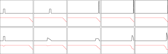
Figure 3. Red traffic light: local case (top panels) vs nonlocal case (bottom panels)

In the local case $v$ does not depend on time, since $u$ is constant. The density $m$ proceeds without changing profile (except some numerical diffusion at the boundary of its support), then starts concentrating close to the traffic light. At the final time, all the mass is concentrated at the point closest to the traffic light.
In the nonlocal case, drivers interactions are clearly visible both in $m$ and $v$. The initial density readily activates the nonlocal term in $v$, and $m$ starts assuming the well known triangle-shaped profile. Close to the traffic light we observe a slowing-down, that propagates backward up to the beginning of the queue, preventing mass concentration. At final time the profile becomes stationary, we observe that $v$ is zero in the whole support of $m$.

We proceed with a test for validating the proposed numerical method. We consider the case of a single switching time $\tau\in[0,T]$, namely we choose $s=(s_{1},s_{2})=(\tau,T-\tau)$ without constraints and $u_{0}=1$, so that the corresponding control is just $u^{s}(t)=\chi_{[0,\tau]}(t)$ (red light on $e_{1}$ for $t\leq\tau$). This reduces the optimization problem to a minimization in dimension one, that can be analyzed by an exaustive search in $\tau$ and then compared with our adjoint-based algorithm. We set all the parameters as in the previous test, in particular we choose constant free flow speeds $v_{1}^{f}=v_{2}^{f}=v_{3}^{f}\equiv 1$ and set $T=1.25$. We also assume that, apart from $m_{0}$, no additional mass enters or leaves the network for all $t\in[0,T]$.

We start with $m_{0}=(m_{0}^{1},m_{0}^{2},m_{0}^{3})=(\chi_{[0.1,0.15]}(x),\chi_{[0.6,0.65]}(x),0)$, i.e. two distributions of equal mass on $e_{1}$ and $e_{2}$ that arrive at the traffic light at different times ($m_{2}$ first and then $m_{1}$). In Figure 4(a) we plot the corresponding (normalized) mean velocity $\bar{v}(\tau)=-J(m,u^{s})/M$ as a function of $\tau$, where $M=\int_{0}^{T}\int_{\Gamma}m(x,t)dx\,dt$.

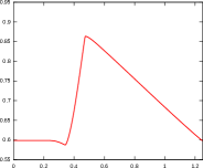
(a)	(b)

Figure 4. Mean velocity for a single switch of the traffic light: well separated $m_{1}$, $m_{2}$ (a), overlapping $m_{1}$, $m_{2}$ (b)

The scenario is pretty clear. If the switch occurs before $m_{2}$ reaches the traffic light, then only $m_{1}$ will move from $e_{1}$ to $e_{3}$ and the mean velocity cannot improve. For larger values of $\tau$, also $m_{2}$ will gradually move to $e_{3}$, and $\bar{v}(\tau)$ increases. If now the switch is placed just after $m_{2}$ leaves $e_{2}$ and before $m_{1}$ approaches the traffic light, we get the best performance, both distributions move as they are on a free road. Note that, due to the nonlocal interactions, the maximum of $\bar{v}$ is less than the free flow speed. Finally, as $\tau$ keeps increasing up to $T$, $m_{1}$ starts getting stuck at the traffic light, and $\bar{v}(\tau)$ decreases.

Now let us repeat the exaustive computation of the mean velocity $\bar{v}(\tau)$ with $m_{0}=(m_{0}^{1},m_{0}^{2},m_{0}^{3})=(\chi_{[0.6,0.65]}(x),\chi_{[0.6,0.65]}(x),0)$, two distributions of equal mass on $e_{1}$ and $e_{2}$, starting at the same distance from the traffic light. Figure 4(b) shows the shape of the corresponding $\bar{v}$. We observe that the maximum of $\bar{v}$ is lower than in the previous test, and it is achieved at a single point instead of an interval. This clearly depends on the fact that the two densities are not well separated as before and it is not possible to place a switch without penalizing the overall traffic flow. Moreover, note that an absolute minimum appears just after the initial plateau. Interestingly, this means that if the switch occurs too early both densities slowdown, whereas the optimal choice corresponds to switch just after $m_{2}$ leaves $e_{2}$ (see Figure 5 below).

These two simple examples show that, in general, the numerical optimization of the traffic light is a very challenging problem, since there is a wide number of local extrema where the gradient descent algorithm can stop. To overcome this issue, we perform several runs with random initial guesses for the controls, and we select the solution obtaining the best result.

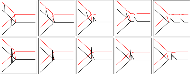
Figure 5. Optimal solutions for well separated densities (top panels) and overlapping densities (bottom panels)

Figure 5 shows two optimal solutions at different times computed by the gradient descent method, both achieving the absolute maximum of the corresponding mean velocity. Top panels refer to the case of well separated densities, bottom panels to the case of overlapping densities. As before, black and red lines represent $m$ and $v$ respectively. The fourth frame in each sequence shows the precise moment of the switch for the traffic light. In the second case we clearly observe that on $e_{1}$ the traffic is stopped until $m_{2}$ leaves $e_{2}$.

We conclude with a more complete example, also including control constraints. All the parameters are the same of the previous tests, but we fix to $S=5$ the number of switching durations (corresponding to $4$ switching times) and we start with $u_{0}=0$, i.e. green light on $e_{1}$. Moreover, we set the constraints $T^{G}=0.15$, $T^{R}=0.3$, and $m_{0}$ is given edge-wise by

$$m^{1}_{0}(x)=\chi_{[0.1,0.15]}(x)+\chi_{[0.4,0.45]}(x)\,,\quad m^{2}_{0}(x)=\chi_{[0.1,0.15]}(x)+\chi_{[0.6,0.65]}(x)\,,\quad m^{3}_{0}(x)=0\,.$$

Note that, with this choice, we are mixing together the two cases analyzed before. Indeed, the initial density consists of four blocks which are, respectively, pairwise overlapped and well separated. The optimal solution produced by the gradient descent algorithm is $s^{*}=(0.227,0.251,0.259,0.3,0.21)$. Figure 6 shows the corresponding evolution at different times.

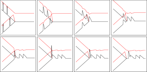
Figure 6. Optimal solution for a traffic light with $4$ switches

We observe that the first switch occurs before $m_{2}$ approaches the traffic light. This allows the first block of $m_{2}$ to proceed without slowdowns from $e_{2}$ to $e_{3}$. The second switch occurs immediately after this block leaves $e_{2}$, so that also the first block of $m_{1}$ can leave $e_{1}$ almost undisturbed before the traffic light switches again. Now, the remaining densities on $e_{1}$ and $e_{2}$ are in overlapping configuration, $m_{2}$ goes first, while $m_{1}$ stops. Finally, the last switch occurs just after $m_{2}$ leaves $e_{2}$, so that also $m_{1}$ can move to $e_{3}$ for the remaining time.

Appendix A Some complementary results for the variational problems

Proof of Lemma 3.1.

Assume without loss of generality that $M=1$. It is well known that for $\mu\in\mathcal{M}^{+}_{M}(\Gamma_{T}),|\mu|_{TV}=\mu(\Gamma_{T})\leq 1.$
By Banach-Alaoglu Theorem it follows the compactness with respect to the weak*-convergence, which implies the same property with respect to the $\|\cdot\|_{BL}^{*}$ convergence. ∎

Lemma 3.2.

Since (3.3) is just a condition which defines the dependence among the components of $u\in\mathcal{U}$, we prove the compactness of

$$\mathcal{U}=\{u\in BV([0,T],\{0,1\})\,\text{and}\,u\,\text{satisfies \eqref{hyp_light1},}\}.$$

Let $(u_{n})_{n\in{\mathbb{N}}}\subset\mathcal{U}$. Denote by $\tau^{n}_{i}$ the switching times of $u_{n}$. By (3.2), for every two consecutive switching times $\tau^{n}_{k},\tau^{n}_{k+1}\in[0,T]$, if $u^{n}(\tau^{n}_{k})=1$, then

$$|\tau^{n}_{k}-\tau^{n}_{k+1}|<T^{R},$$

otherwise,

$$|\tau^{n}_{k}-\tau^{n}_{k+1}|>T^{G}.$$

Since $u_{n}(t)\in\{0,1\}$, we can assume that there exists a subsequence, still denoted by $u_{n}$, such that either $u_{n}(0)=1$ or $u_{n}(0)=0$ for every $n\in{\mathbb{N}}$. Assume now that, w.l.o.g., $u_{n}(0)=1$ for every $n\in{\mathbb{N}}$ and denote by $I_{n}$ the set of switching times of $u_{n}$. It follows that

$$\frac{T}{T^{R}}\leq\#(I_{n})\leq\frac{T}{T^{G}}.$$

As before, we can assume, w.l.o.g., that that there exists $N\in{\mathbb{N}}$ such that $\#(I_{n})=N$ for all $n\in{\mathbb{N}}$. Since $I_{n}\subset[0,T]$, applying the Cantor diagonal procedure, it follows that there exists a subsequence $(I_{n_{k}})_{k\in{\mathbb{N}}}$ such that $\tau_{i}^{n_{k}}\to\tau_{i}$ for $i=1,\ldots,N$. In this way, we define a candidate $u$ as limit for the subsequence $u_{n_{k}}$ from the switching times set $\{\tau_{1},\ldots,\tau_{N}\}$ and $u(0)=1$. To conclude, we only need to show that $u_{n_{k}}\to u$ in $L^{1}$. By construction,

$$\|u_{n_{k}}-u\|_{L^{1}}=\sum_{i=1}^{N}|\tau_{i}^{n_{k}}-\tau_{i}|\leq N\sup_{i=1,\ldots,N}|\tau_{i}^{n_{k}}-\tau_{i}|\to_{k\to\infty}0$$

∎

Proof of Lemma 3.3 (traffic lights).

In this case, the distirbution $\mu$ has no role since it depends exclusively on $u$. Hence, we reduce on $\mathcal{X}=\mathcal{M}^{+}(\Gamma_{T})\times\mathcal{U},$ where $\mathcal{U}$ defined by (3.4).
Let $(m_{n},u_{n})_{n\in{\mathbb{N}}}\subset A$ such that $(m_{n},u_{n})\to(m,u)$ with respect the norm $\|\cdot\|_{BL}^{*}+\|\cdot\|_{L^{1}}.$
The closure on the first component derives from the proof of Lemma 4.1 in [4] and the results in [7].
Instead, the closure on the second component derives from the compactness of $\mathcal{U}$. Indeed, there exists a subsequence $(u_{n_{k}})_{k\in{\mathbb{N}}}$ which converges to $\tilde{u}\in\mathcal{U}$, but it also converges to $u$ by assumption. Then, it follows that $u=\tilde{u}\in\mathcal{U}.$

∎

Proof of Lemma 3.4 (autonomous cars).

It follows adopting the argument in the previous proof, for $\mathcal{X}=\mathcal{M}^{+}_{M}(\Gamma_{T})\times\mathcal{M}^{+}_{M}(\Gamma_{T})\times\mathcal{U}$ endowed with the norm $\|\cdot\|_{BL}^{*}+\|\cdot\|_{BL}^{*}+\|\cdot\|_{\infty}.$

∎

References

- [1] L. Ambrosio, N. Gigli, G. Savaré, Gradient ows in metric spaces and in the space of probability measures, Lectures in Mathematics ETH Zürich, Birkhäuser Verlag, Basel, 2008.
- [2] G. Albi, M. Bongini, E. Cristiani, D. Kalise, Invisible control of self-organizing agents leaving unknown environments, SIAM J. Appl. Math., 76 (2016), 1683-1710.
- [3] N. Bellomo, B. Piccoli, A. Tosin, Modeling crowd dynamics from a complex system viewpoint, Math. Models Methods Appl. Sci., 22 (Supp. 2) (2012), 1230004.
- [4] M. Bongini, G. Buttazzo, Optimal control problems in transport dynamics, Math. Models Methods Appl. Sci. 27 (2017), 427-451.
- [5] A. Bressan, S. Čanić, M. Garavello, M. Herty, B. Piccoli, Flows on networks: recent results and perspectives, EMS Surv. Math. Sci. 1 (2014), no. 1, 47-111.
- [6] F. Camilli, R. De Maio, A. Tosin, Transport of measures on networks, Netw. Heterog. Media, 12 (2017), 191 - 215.
- [7] F. Camilli, R. De Maio, A. Tosin, Measure-valued solutions to transport equations on networks with nonlocal velocity, J. Differential Equations (in press) 2018.
- [8] J. A. Cañizo, J. A. Carrillo, J. Rosado, A well-posedness theory in measures for some kinetic models of collective motion, Math. Models Methods Appl. Sci. 21 (2011), no. 3, 515-539.
- [9] E. Cascetta, Transportation Systems Analysis, Springer, Heidelberg (2009).
- [10] G.Cavagnari, A.Marigonda, B.Piccoli, Averaged time-optimal control problem in the space of positive Borel measures, Esaim COCV (2018), in press.
- [11] G. Cavagnari, A. Marigonda, K.T. Nguyen, F.S. Priuli,Generalized control systems in the space of probability measures, Set-Valued Var. Anal. (2017), 1 - 29.
- [12] R. M. Colombo, M. Garavello, M. Léecureux-Mercier, A class of nonlocal models for pedestrian traffic, Math. Models Methods Appl. Sci. 22 (2012), no. 4, 1150023.
- [13] F. Cucker and S. Smale, Emergent behaviour in flocks, IEEE Trans. on Auto. Con. 52 (2007), 852–862.
- [14] M. Garavello, K. Han, B. Piccoli, Models for vehicular traffic on networks, AIMS Series on Applied Mathematics, American Institute of Mathematical Sciences, Springfield, MO, 2016.
- [15] V. Trozzi , I. Kaparias , M. G.H. Bell, G. Gentile, A dynamic route choice model for public transport networks with boarding queues, Trans. Plan. and Tech. 36 (20113), 44-61.
- [16] G. Gentile, L. Meschini, Using dynamic assignment models for real-time traffic forecast on large urban networks, in “2nd Int. Conf. on Mod. and Tech. for Int. Trans. Sys.”, Leuven, Belgium (2011).
- [17] S. Gottlich, U. Ziegler, Traffic light control: a case study, Dis. and Con. Dyn. Sys. 7 (2014), 483–501.
- [18] R. Wang, Y. Li, D. B. Work, Comparing traffic state estimators for mixed human and automated traffic flows, Transportation Research Part C: Emerging Technologies 78 (2017), 95–110.