A nonlinear Stokes-Biot model for the interaction of a non-Newtonian fluid with poroelastic media

Abstract

We develop and analyze a model for the interaction of a quasi-Newtonian free fluid with a poroelastic medium. The flow in the fluid region is described by the nonlinear Stokes equations and in the poroelastic medium by the nonlinear quasi-static Biot model. Equilibrium and kinematic conditions are imposed on the interface. We establish existence and uniqueness of a solution to the weak formulation and its semidiscrete continuous-in-time finite element approximation. We present error analysis, complemented by numerical experiments.

1 Introduction

The interaction of a free fluid with a deformable porous medium is a challenging multiphysics problem that has a wide range of applications, including processes arising in gas and oil extraction from naturally or hydraulically fractured reservoirs, designing industrial filters, and blood-vessel interactions. The free fluid region can be modeled by the Stokes or the Navier-Stokes equations, while the flow through the deformable porous medium is modeled by the quasi-static Biot system of poroelasticity [5]. The two regions are coupled via dynamic and kinematic interface conditions, including balance of forces, continuity of normal velocity, and a no slip or slip with friction tangential velocity condition. These multiphysics models exhibit features of coupled Stokes-Darcy flows and fluid-structure interaction (FSI). There is extensive literature on modeling these separate couplings, see e.g. [19, 32, 39] for Stokes-Darcy flows and [25, 24, 27] for FSI. More recently there has been growing interest in modeling Stokes-Biot couplings, which can be referred to as fluid-poroelastic structure interaction (FPSI). The well-posedness of the mathematical model is studied in [43]. A variational multiscale stabilized finite element method for the Navier-Stokes-Biot problem is developed in [3]. In [11] a non-iterative operator-splitting method is developed for the Navier-Stokes-Biot model with pressure Darcy formulation. The well posedness of a related model is studied in [14]. The Stokes-Biot problem with a mixed Darcy formulation is studied in [10] and [2] using Nitsche’s method and a Lagrange multiplier, respectively, to impose the continuity of normal velocity on the interface. An optimization-based iterative algorithm with Neumann control is proposed in [15]. A reduced-dimension fracture model coupling Biot and an averaged Brinkman equation is developed in [12]. Alternative fracture models using the Reynolds lubrication equation coupled with Biot have also been studied, see e.g. [28].

All of the above mentioned works are based on Newtonian fluids. In this paper we develop FPSI with non-Newtonian fluids, which, to the best of our knowledge, has not been studied in the literature. In many applications the fluid exhibits properties that cannot be captured by a Newtonian fluid assumption. For instance, during water flooding in oil extraction, polymeric solutions are often added to the aqueous phase to increase its viscosity, resulting in a more stable displacement of oil by the injected water [34]. In hydraulic fracturing, proppant particles are mixed with polymers to maintain high permeability of the fractured media [33]. In blood flow simulations of small vessels or for patients with a cardiovascular disease, where the arterial geometry has been altered to include regions of re-circulation, one needs to consider models that can capture the sheer-thinning property of the blood [31].

In this work we use nonlinear Stokes equations to model the free fluid in the flow region and a nonlinear Biot model for the fluid in the poroelastic region. Our model is built on the nonlinear Stokes-Darcy model presented in [22] and the linear Stokes-Biot model considered in [2]. Our Biot model is based on a linear stress-strain constitutive relationship and a nonlinear Darcy flow. The coupling conditions between the two subdomains include mass conservation, conservation of momentum and the Beavers-Joseph-Saffman slip with friction condition. We focus on fluids that possess the sheer thinning property, i.e., the viscosity decreases under shear strain, which is typical for polymer solutions and blood. Viscosity models for such non-Newtonian fluids include the Power law, the Cross model and the Carreau model [6, 16, 36, 34, 37]. The Power law model is popular because it only contains two parameters, and it is possible to derive analytical solutions in various flow conditions [6]. On the other hand, it implies that in the flow region the viscosity goes to infinity if the deformation goes to zero, which may not be representative in certain applications. The Cross and Carreau models have been deduced empirically as alternatives of the Power law model. They have three parameters, and in some parameter regimes, the viscosity is strictly greater than zero and bounded. We assume that the viscosity in each subdomain satisfies one such model, with dependence on the magnitude of the deformation tensor and the magnitude of Darcy velocity in the fluid and poroelastic regions, respectively. We further assume that along the interface the fluid viscosity is a function of the fluid and structure interface velocities. We consider both unbounded and bounded parameter regimes. In the former case, the analysis is done in an appropriate Sobolev space setting, using spaces such as $W^{1,r}$, where $1<r<2$ is the viscosity shear thinning parameter. In the latter case, the analysis reduces to the Hilbert space setting. Nonlinear Stokes-Darcy models with bounded viscosity have been studied in [23, 20, 13], while the unbounded case is considered in [22].

Following the approach in [2], we enforce the continuity of normal velocity on the interface through the use of a Lagrange multiplier. The resulting weak formulation is a nonlinear time-dependent system, which is difficult to analyze, due to to the presence of the time derivative of the displacement in some non-coercive terms. We consider an alternative mixed elasticity formulation with the structure velocity and elastic stress as primary variables, see also [43]. In this case we obtain a system with a degenerate evolution in time operator and a nonlinear saddle-point type spatial operator. The structure of the problem is similar to the one analyzed in [44], see also [8] in the linear case. However, the analysis in [44] is restricted to the Hilbert space setting and needs to be extended to the Sobolev space setting. Furthermore, the analysis in [44] is for monotone operators, see [45], and as a result requires certain right hand side terms to be zero, while in typical applications these terms may not be zero. Here we explore the coercivity of the operators to reformulate the problem as a parabolic-type system for the pressure and stress in the poroelastic region. We show well posedness for this system for general source terms and that the solution satisfies the original formulation. We also prove that the solution to the original formulation is unique and provide a stability bound. We then consider a semidiscrete finite element approximation of the system and carry out stability and error analysis. For this purpose we establish a discrete inf-sup condition, which involves a non-conforming Lagrange multiplier discretization that allows for non-matching grids across the Stokes-Biot interface.

The rest of the paper is organized as follows. In Section 2 we introduce the governing equations. Section 3 is devoted to the weak formulation, upon which we base the numerical method, and an alternative formulation, which is needed for the purpose of the analysis. In Section 4 we prove the well-posedness of the alternative and original formulations. The semidiscrete approximation and its well-posedness analysis are developed in Section 5. The error analysis is carried out in Section 6. Numerical experiments are presented in Section 7.

2 Problem set-up

Let $\Omega\subset\mathbb{R}^{d},\,d=2,3$ be a Lipschitz domain, which is subdivided into two non-overlapping and possibly non-connected regions: fluid region $\Omega_{f}$ and poroelastic region $\Omega_{p}$. Let $\partial\Omega_{f}\cap\partial\Omega_{p}=\Gamma_{fp}$ denote the (nonempty) interface between these regions and let $\Gamma_{f}=\partial\Omega_{f}\setminus\Gamma_{fp}$ and $\Gamma_{p}=\partial\Omega_{p}\setminus\Gamma_{fp}$ denote the external parts of the boundary $\partial\Omega$. We denote by ${\bf n}_{f}$ and ${\bf n}_{p}$ he unit normal vectors which point outward from $\partial\Omega_{f}$ and $\partial\Omega_{p}$, respectively, noting that ${\bf n}_{f}=-{\bf n}_{p}$ on $\Gamma_{fp}$. Let $({\bf u}_{\star},p_{\star})$ be the velocity-pressure pairs in $\Omega_{\star}$, $\star=f$, $p$, and let $\mbox{{\boldmath$\eta$}}_{p}$ be the displacement in $\Omega_{p}$.

We assume that the flow in $\Omega_{f}$ is governed by the nonlinear generalized Stokes equations with homogeneous boundary conditions on $\Gamma_{f}$:

$$-\nabla\cdot\mbox{{\boldmath$\sigma$}}_{f}({\bf u}_{f},p_{f})={\bf f}_{f},\quad\nabla\cdot{\bf u}_{f}=q_{f}\quad\mbox{in }\Omega_{f}\times(0,T],\quad{\bf u}_{f}={\bf 0}\quad\mbox{on }\Gamma_{f}\times(0,T],$$ (2.1)

where ${\bf D}({\bf u}_{f})$ and $\mbox{{\boldmath$\sigma$}}_{f}({\bf u}_{f},p_{f})$ denote the deformation and the stress tensors, respectively:

$${\bf D}({\bf u}_{f})=\frac{1}{2}(\nabla{\bf u}_{f}+\nabla{\bf u}_{f}^{T}),\quad\mbox{{\boldmath$\sigma$}}_{f}({\bf u}_{f},p_{f})=-p_{f}{\bf I}+2\nu({\bf D}({\bf u}_{f})){\bf D}({\bf u}_{f}),$$

where ${\bf I}$ stands for the identity operator. We consider a generalized Newtonian fluid with the viscosity $\nu$ dependent on the magnitude of the deformation tensor, in particular shear-thinning fluids with $\nu$ a decreasing function of $|{\bf D}({\bf u}_{f})|$. We consider the following models [16, 36], where $1<r<2$, $0\leq\nu_{\infty}<\nu_{0}$, and $K_{f}>0$ are constants:

Carreau model:

$$\nu({\bf D}({\bf u}_{f}))=\nu_{\infty}+(\nu_{0}-\nu_{\infty})/(1+K_{f}|{\bf D}({\bf u}_{f})|^{2})^{(2-r)/2},$$ (2.2)

Cross model:

$$\nu({\bf D}({\bf u}_{f}))=\nu_{\infty}+(\nu_{0}-\nu_{\infty})/(1+K_{f}|{\bf D}({\bf u}_{f})|^{2-r}),$$ (2.3)

Power law model:

$$\nu({\bf D}({\bf u}_{f}))=K_{f}|{\bf D}({\bf u}_{f})|^{r-2}.$$ (2.4)

In turn, in $\Omega_{p}$ we consider the quasi-static Biot system [5]

$$-\nabla\cdot\mbox{{\boldmath$\sigma$}}_{p}(\mbox{{\boldmath$\eta$}}_{p},p_{p})={\bf f}_{p}\quad\mbox{in }\Omega_{p}\times(0,T],$$ (2.5)

$$\nu_{eff}({\bf u}_{p})\kappa^{-1}{\bf u}_{p}+\nabla p_{p}=0,\quad\frac{\partial}{\partial t}(s_{0}p_{p}+\alpha_{p}\nabla\cdot\mbox{{\boldmath$\eta$}}_{p})+\nabla\cdot{\bf u}_{p}=q_{p}\quad\mbox{in }\Omega_{p}\times(0,T],$$ (2.6)

$${\bf u}_{p}\cdot{\bf n}_{p}=0\,\mbox{ on }\,\Gamma_{p}^{N}\times(0,T],\quad p_{p}=0\,\mbox{ on }\Gamma_{p}^{D}\times(0,T],\quad\mbox{{\boldmath$\eta$}}_{p}={\bf 0}\mbox{ on }\Gamma_{p}\times(0,T],$$ (2.7)

where $\mbox{{\boldmath$\sigma$}}_{e}(\mbox{{\boldmath$\eta$}}_{p})$ and $\mbox{{\boldmath$\sigma$}}_{p}(\mbox{{\boldmath$\eta$}}_{p},p_{p})$ are the elasticity and poroelasticity stress tensors, respectively,

$$\mbox{{\boldmath$\sigma$}}_{e}(\mbox{{\boldmath$\eta$}}_{p})=\lambda_{p}(\nabla\cdot\mbox{{\boldmath$\eta$}}_{p}){\bf I}+2\mu_{p}{\bf D}(\mbox{{\boldmath$\eta$}}_{p}),\quad\mbox{{\boldmath$\sigma$}}_{p}(\mbox{{\boldmath$\eta$}}_{p},p_{p})=\mbox{{\boldmath$\sigma$}}_{e}(\mbox{{\boldmath$\eta$}}_{p})-\alpha_{p}p_{p}{\bf I},$$ (2.8)

$\alpha_{p}$ is the Biot-Willis constant, $\lambda_{p}$, $\mu_{p}$ are the Lamè coefficients, $s_{0}>0$ is a storage coefficient, $\kappa$ is a scalar uniformly positive and bounded permeability function, and $\Gamma_{p}=\Gamma_{p}^{N}\cup\Gamma_{p}^{D}$. To avoid the issue with restricting the mean value of the pressure, we assume that $|\Gamma_{p}^{D}|>0$. We further assume that $\mbox{dist}(\Gamma_{p}^{D},\Gamma_{fp})\geq s>0$. We note that even though the analysis of our formulation is valid for a symmetric and positive definite permeability tensor, we restrict it to $\kappa{\bf I}$, due to assumptions made in the derivations of some of the viscosity functions suitable for modeling non-Newtonian flow in porous media. In particular, we consider the following two models for the effective viscosity $\nu_{eff}$ in $\Omega_{p}$ [34, 37], where $1<r<2$, $0\leq\nu_{\infty}<\nu_{0}$, and $K_{p}>0$ are constants:

Cross model:

$$\nu_{eff}({\bf u}_{p})=\nu_{\infty}+(\nu_{0}-\nu_{\infty})/(1+K_{p}|{\bf u}_{p}|^{2-r}),$$ (2.9)

Power law model:

$$\nu_{eff}({\bf u}_{p})=K_{p}(|{\bf u}_{p}|/(\sqrt{\kappa}m_{c}))^{r-2},$$ (2.10)

where $m_{c}$ is a constant that depends on the internal structure of the porous media.

Following [43, 3], the interface conditions on the fluid-poroelasticity interface $\Gamma_{fp}$, are mass conservation, balance of normal stress, the Beavers-Joseph-Saffman (BJS) slip with friction condition [4, 40], and conservation of momentum:

$${\bf u}_{f}\cdot{\bf n}_{f}+\left(\frac{\partial\mbox{{\boldmath$\eta$}}_{p}}{\partial t}+{\bf u}_{p}\right)\cdot{\bf n}_{p}=0\quad\mbox{on }\Gamma_{fp},$$ (2.11)

$$-(\mbox{{\boldmath$\sigma$}}_{f}{\bf n}_{f})\cdot{\bf n}_{f}=p_{p}\quad\mbox{on }\Gamma_{fp},$$ (2.12)

$$-(\mbox{{\boldmath$\sigma$}}_{f}{\bf n}_{f})\cdot{\bf t}_{f,j}=\nu_{I}\,\alpha_{BJS}\sqrt{\kappa^{-1}}\left({\bf u}_{f}-\frac{\partial\mbox{{\boldmath$\eta$}}_{p}}{\partial t}\right)\cdot{\bf t}_{f,j}\quad\mbox{on }\Gamma_{fp},$$ (2.13)

$$\mbox{{\boldmath$\sigma$}}_{f}{\bf n}_{f}=-\mbox{{\boldmath$\sigma$}}_{p}{\bf n}_{p}\quad\mbox{on }\Gamma_{fp},$$ (2.14)

where ${\bf t}_{f,j}$, $1\leq j\leq d-1$, is an orthogonal system of unit tangent vectors on $\Gamma_{fp}$ and $\alpha_{BJS}\geq 0$ is an experimentally determined friction coefficient. We note that the continuity of flux takes into account the normal velocity of the solid skeleton, while the BJS condition accounts for its tangential velocity. We assume that along the interface the fluid viscosity $\nu_{I}$ is a function of the magnitude of the tangential component of the slip velocity $\left|\sum_{j=1}^{d-1}(({\bf u}_{f}-\partial_{t}\mbox{{\boldmath$\eta$}}_{p})\cdot{\bf t}_{f,j}){\bf t}_{f,j}\right|$ given by the Cross model (2.9) or the Power law model (2.10), where $\partial_{t}\phi:=\partial\phi/\partial t$. For the rest of the paper we will write $\nu$, $\nu_{eff}$ or $\nu_{I}$ keeping in mind that these are nonlinear functions as defined above.

The above system of equations is complemented by a set of initial conditions:

$$p_{p}(0,\mathbf{x})=p_{p,0}(\mathbf{x}),\,\,\mbox{{\boldmath$\eta$}}_{p}(0,\mathbf{x})=\mbox{{\boldmath$\eta$}}_{p,0}(\mathbf{x})\mbox{ in }\Omega_{p}.$$

In the following, we make use of the usual notation for Lebesgue spaces $L^{p}(\Omega)$, Sobolev spaces $W^{k,p}(\Omega)$ and Hilbert spaces $H^{k}(\Omega)$. For a set ${{\mathcal{O}}}\subset\mathbb{R}^{d}$, the $L^{2}({{\mathcal{O}}})$ inner product is denoted by $(\cdot,\cdot)_{{{\mathcal{O}}}}$ for scalar, vector and tensor valued functions. For a section of a subdomain boundary $S$ we write $\langle\cdot,\cdot\rangle_{S}$ for the $L^{2}(S)$ inner product (or duality pairing). We also denote by $C$ a generic positive constant independent of the discretization parameters.

Adopting the approach from [22, 23], we assume that the viscosity functions satisfy one of the two sets of assumptions (A1)–(A2) or (B1)–(B2) below. Let $g({\bf x}):\mathbb{R}^{d}\rightarrow\mathbb{R}^{+}\cup\{0\}$ and let ${\bf G}({\bf x}):\mathbb{R}^{d}\rightarrow\mathbb{R}^{d}$ be given by ${\bf G}({\bf x})=g({\bf x}){\bf x}$. For ${\bf x},{\bf h}\in\mathbb{R}^{d}$, let ${\bf G}({\bf x})$ satisfy, for constants $C_{1},\ldots,C_{4}>0$ and $c\geq 0$,

$$\left({\bf G}({\bf x}+{\bf h})-{\bf G}({\bf x})\right)\cdot{\bf h} \geq C_{1}|{\bf h}|^{2},$$ (A1)

$$|{\bf G}({\bf x}+{\bf h})-{\bf G}({\bf x})| \leq C_{2}|{\bf h}|,$$ (A2)

or

$$({\bf G}({\bf x}+{\bf h})-{\bf G}({\bf x}))\cdot{\bf h} \geq C_{3}\frac{|{\bf h}|^{2}}{c+|{\bf x}|^{2-r}+|{\bf x}+{\bf h}|^{2-r}},$$ (B1)

$$|{\bf G}({\bf x}+{\bf h})-{\bf G}({\bf x})| \leq C_{4}\frac{|{\bf h}|}{c+|{\bf x}|^{2-r}+|{\bf x}+{\bf h}|^{2-r}},$$ (B2)

with the convention that ${\bf G}({\bf x})={\bf 0}$ if ${\bf x}={\bf 0}$, and $|{\bf h}|/(c+|{\bf x}|+|{\bf h}|)=0$ if $c=0$ and ${\bf x}={\bf h}={\bf 0}$. From (B1)–(B2) it follows that there exist constants $C_{5},C_{6}>0$ such that for ${\bf s},{\bf t},{\bf w}\in(L^{r}({{\mathcal{O}}}))^{d}$ [41]

$$({\bf G}({\bf s})-{\bf G}({\bf t}),{\bf s}-{\bf t})_{{{\mathcal{O}}}}\geq C_{5}\left((|{\bf G}({\bf s})-{\bf G}({\bf t})|,|{\bf s}-{\bf t}|)_{{{\mathcal{O}}}}+\frac{\|{\bf s}-{\bf t}\|^{2}_{L^{r}({{\mathcal{O}}})}}{c+\|{\bf s}\|^{2-r}_{L^{r}({{\mathcal{O}}})}+\|{\bf t}\|^{2-r}_{L^{r}({{\mathcal{O}}})}}\right),$$ (2.15)

$$({\bf G}({\bf s})-{\bf G}({\bf t}),{\bf w})_{{{\mathcal{O}}}}\leq C_{6}\left\|\frac{|{\bf s}-{\bf t}|}{c+|{\bf s}|+|{\bf t}|}\right\|^{\frac{2-r}{r}}_{L^{\infty}({{\mathcal{O}}})}(|{\bf G}({\bf s})-{\bf G}({\bf t})|,|{\bf s}-{\bf t}|)_{{{\mathcal{O}}}}^{1/r^{\prime}}\|{\bf w}\|_{L^{r}({{\mathcal{O}}})}.$$ (2.16)

Remark 2.1.

It is shown in [20] that conditions (A1)–(A2) are satisfied for $g({\bf D}({\bf u}_{f}))=\nu({\bf D}({\bf u}_{f}))$ given in the Carreau model (2.2) with $\nu_{\infty}>0$, in which case $\nu_{\infty}\leq g({\bf x})\leq\nu_{0}$. A similar argument can be applied to show that (A1)–(A2) hold for the Cross model, with $g({\bf D}({\bf u}_{f}))=\nu({\bf D}({\bf u}_{f}))$ given in (2.3) for Stokes and $g({\bf u}_{p})=\nu_{eff}({\bf u}_{p})$ given in (2.9) for Darcy, in the case of $\nu_{\infty}>0$. Furthermore, it is shown in [41] that conditions (B1)–(B2) with $c>0$ hold in the case of the Carreau model (2.2) with $\nu_{\infty}=0$, and that conditions (B1)–(B2) with $c=0$ hold for the Power law model (2.4) and (2.10).

3 Variational formulation

We will consider two cases when defining the functional spaces, depending on which set of assumptions holds. In the case (B1)–(B2), we consider Sobolev spaces. For a given $r>1$ let $r^{\prime}$ be its conjugate, satisfying $r^{-1}+(r^{\prime})^{-1}=1$. Let

$${\bf V}_{f} =\{{\bf v}_{f}\in(W^{1,r}(\Omega_{f}))^{d}:{\bf v}_{f}={\bf 0}\text{ on }\Gamma_{f}\}, W_{f}=L^{r^{\prime}}(\Omega_{f}),$$ (3.1)

with the corresponding norms

$$\|{\bf v}_{f}\|_{{\bf V}_{f}}=\|{\bf v}_{f}\|_{(W^{1,r}(\Omega_{f}))^{d}},\quad\|w_{f}\|_{W_{f}}=\|w_{f}\|_{L^{r^{\prime}}(\Omega_{f})}.$$

With $L^{r}(\text{div};\Omega_{p})=\{{\bf v}_{p}\in(L^{r}(\Omega_{p}))^{d}:\nabla\cdot{\bf v}_{p}\in L^{r}(\Omega_{p})\}$, let

$${\bf V}_{p} =\{{\bf v}_{p}\in L^{r}(\text{div};\Omega_{p}):{\bf v}_{p}\cdot{\bf n}_{p}=0\text{ on }\Gamma^{N}_{p}\}, W_{p}=L^{r^{\prime}}(\Omega_{p}),$$

$${\bf X}_{p} =\{\mbox{{\boldmath$\xi$}}_{p}\in(H^{1}(\Omega_{p}))^{d}:\mbox{{\boldmath$\xi$}}_{p}={\bf 0}\text{ on }\Gamma_{p}\}.$$ (3.2)

with norms

$$\|{\bf v}_{p}\|^{r}_{{\bf V}_{p}} =\|{\bf v}_{p}\|^{r}_{(L^{r}(\Omega_{p}))^{d}}+\|\nabla\cdot{\bf v}_{p}\|^{r}_{L^{r}(\Omega_{p})}, \|w_{p}\|_{W_{p}}=\|w_{p}\|_{L^{r^{\prime}}(\Omega_{p})},$$

$$\|\mbox{{\boldmath$\eta$}}_{p}\|_{{\bf X}_{p}} =\|\mbox{{\boldmath$\eta$}}_{p}\|_{(H^{1}(\Omega_{p}))^{d}}.$$

In the case of (A1)–(A2), we consider Hilbert spaces, with the above definitions replaced by

$${\bf V}_{f} =\{{\bf v}_{f}\in(H^{1}(\Omega_{f}))^{d}:{\bf v}_{f}={\bf 0}\text{ on }\Gamma_{f}\}, W_{f}=L^{2}(\Omega_{f}),$$ (3.3)

$${\bf V}_{p} =\{{\bf v}_{p}\in H(\text{div};\Omega_{p}):{\bf v}_{p}\cdot{\bf n}_{p}=0\text{ on }\Gamma^{N}_{p}\}, W_{p}=L^{2}(\Omega_{p}).$$ (3.4)

The global spaces are products of the subdomain spaces. For simplicity we assume that each region consists of a single subdomain.

Remark 3.1.

For simplicity of the presentation, for the rest of the paper we focus on the case (B1)–(B2), which is the technically more challenging case. The arguments apply directly to the case (A1)–(A2).

3.1 Lagrange multiplier formulation

To derive the weak formulation, we multiply (2.1), (2.5)–(2.6) by appropriate test functions and integrate each equation over the corresponding region, utilizing the boundary and interface conditions (2.11)–(2.14). Integration by parts in the first equation in (2.1), (2.5), and the first equation in (2.6) leads to the Stokes, Darcy and the elasticity functionals

$$a_{f}(\cdot,\cdot)\,:\,{\bf V}_{f}\times{\bf V}_{f}\,\longrightarrow\,\mathbb{R},\quad\quad a_{f}({\bf u}_{f},{\bf v}_{f}) :=(2\nu{\bf D}({\bf u}_{f}),{\bf D}({\bf v}_{f}))_{\Omega_{f}},$$

$$a^{d}_{p}(\cdot,\cdot)\,:\,{\bf V}_{p}\times{\bf V}_{p}\,\longrightarrow\,\mathbb{R},\quad\quad a^{d}_{p}({\bf u}_{p},{\bf v}_{p}) :=(\nu_{eff}\kappa^{-1}{\bf u}_{p},{\bf v}_{p})_{\Omega_{p}},$$

$$a^{e}_{p}(\cdot,\cdot)\,:\,{\bf X}_{p}\times{\bf X}_{p}\,\longrightarrow\,\mathbb{R},\quad\quad a^{e}_{p}(\mbox{{\boldmath$\eta$}}_{p},\mbox{{\boldmath$\xi$}}_{p}) :=(2\mu_{p}{\bf D}(\mbox{{\boldmath$\eta$}}_{p}),{\bf D}(\mbox{{\boldmath$\xi$}}_{p}))_{\Omega_{p}}+(\lambda_{p}\nabla\cdot\mbox{{\boldmath$\eta$}}_{p},\nabla\cdot\mbox{{\boldmath$\xi$}}_{p})_{\Omega_{p}},$$

the bilinear forms

$$b_{\star}(\cdot,\cdot)\,:\,{\bf V}_{\star}\times W_{\star}\,\longrightarrow\,\mathbb{R},\quad\quad b_{\star}({\bf v},w):=-(\nabla\cdot{\bf v},w)_{\Omega_{\star}},\quad\star=f,p,$$

and the interface term

$$I_{\Gamma_{fp}}=-\langle\mbox{{\boldmath$\sigma$}}_{f}{\bf n}_{f},{\bf v}_{f}\rangle_{\Gamma_{fp}}-\langle\mbox{{\boldmath$\sigma$}}_{p}{\bf n}_{p},\mbox{{\boldmath$\xi$}}_{p}\rangle_{\Gamma_{fp}}+\langle p_{p},{\bf v}_{p}\cdot{\bf n}_{p}\rangle_{\Gamma_{fp}}.$$

This term is incorporated into the weak formulation by introducing a Lagrange multiplier which has a meaning of normal stress/Darcy pressure on the interface:

$$\lambda=-(\mbox{{\boldmath$\sigma$}}_{f}{\bf n}_{f})\cdot{\bf n}_{f}=p_{p},\qquad\mbox{on }\Gamma_{fp}.$$

With $\lambda$ introduced, we have, using (2.12), (2.13) and (2.14),

$$I_{\Gamma_{fp}}=a_{BJS}({\bf u}_{f},\partial_{t}\mbox{{\boldmath$\eta$}}_{p};{\bf v}_{f},\mbox{{\boldmath$\xi$}}_{p})+b_{\Gamma}({\bf v}_{f},{\bf v}_{p},\mbox{{\boldmath$\xi$}}_{p};\lambda),$$

where

$$a_{BJS}({\bf u}_{f},\mbox{{\boldmath$\eta$}}_{p};{\bf v}_{f},\mbox{{\boldmath$\xi$}}_{p}) =\sum_{j=1}^{d-1}\big{\langle}\nu_{I}\,\alpha_{BJS}\sqrt{\kappa^{-1}}({\bf u}_{f}-\mbox{{\boldmath$\eta$}}_{p})\cdot{\bf t}_{f,j},({\bf v}_{f}-\mbox{{\boldmath$\xi$}}_{p})\cdot{\bf t}_{f,j}\big{\rangle}_{\Gamma_{fp}},$$

$$b_{\Gamma}({\bf v}_{f},{\bf v}_{p},\mbox{{\boldmath$\xi$}}_{p};\mu) =\langle{\bf v}_{f}\cdot{\bf n}_{f}+(\mbox{{\boldmath$\xi$}}_{p}+{\bf v}_{p})\cdot{\bf n}_{p},\mu\rangle_{\Gamma_{fp}}.$$

For the term $b_{\Gamma}({\bf v}_{f},{\bf v}_{p},\mbox{{\boldmath$\xi$}}_{p};\lambda)$ to be well-defined, we choose the Lagrange multiplier space as $\Lambda=W^{1/r,r^{\prime}}(\Gamma_{fp})$. It is shown in [22] that in the case $\mbox{dist}(\Gamma_{p}^{D},\Gamma_{fp})\geq s>0$, if ${\bf v}_{p}\in L^{r}(\text{div};\Omega_{p})$, then ${\bf v}_{p}\cdot{\bf n}_{p}|_{\Gamma_{fp}}$ can be identified with a functional in $W^{-1/r,r}(\Gamma_{fp})$. Furthermore, for ${\bf v}_{f}\in W^{1,r}(\Omega_{f})$, ${\bf v}_{f}\cdot{\bf n}_{f}\in W^{1/r^{\prime},r}(\partial\Omega_{f})$, and for $\mbox{{\boldmath$\xi$}}_{p}\in H^{1}(\Omega_{p})\subset W^{1,r}(\Omega_{p})$, $\mbox{{\boldmath$\xi$}}_{p}\cdot{\bf n}_{p}\in W^{1/r^{\prime},r}(\partial\Omega_{p})$. Therefore, with $\mu\in W^{1/r,r^{\prime}}(\Gamma_{fp})$, the integrals in $b_{\Gamma}({\bf v}_{f},{\bf v}_{p},\mbox{{\boldmath$\xi$}}_{p};\lambda)$ are well-defined.

The variational formulation reads: given ${\bf f}_{f}\in W^{1,1}(0,T;{\bf V}_{f}^{\prime})$, ${\bf f}_{p}\in W^{1,1}(0,T;{\bf X}_{p}^{\prime})$, $q_{f}\in W^{1,1}(0,T;W_{f}^{\prime})$, $q_{p}\in W^{1,1}(0,T;W_{p}^{\prime})$, and $p_{p}(0)=p_{p,0}\in W_{p}$, $\mbox{{\boldmath$\eta$}}_{p}(0)=\mbox{{\boldmath$\eta$}}_{p,0}\in{\bf X}_{p}$, find, for $t\in(0,T]$, $({\bf u}_{f}(t),p_{f}(t),{\bf u}_{p}(t),p_{p}(t),$ $\mbox{{\boldmath$\eta$}}_{p}(t),\lambda(t))\in L^{\infty}(0,T;{\bf V}_{f})\times L^{\infty}(0,T;W_{f})\times L^{\infty}(0,T;{\bf V}_{p})\times W^{1,\infty}(0,T;W_{p})\times W^{1,\infty}(0,T;{\bf X}_{p})$ $\times L^{\infty}(0,T;\Lambda)$, such that for all ${\bf v}_{f}\in{\bf V}_{f}$, $w_{f}\in W_{f}$, ${\bf v}_{p}\in{\bf V}_{p}$, $w_{p}\in W_{p}$, $\mbox{{\boldmath$\xi$}}_{p}\in{\bf X}_{p}$, and $\mu\in\Lambda$,

$$a_{f}({\bf u}_{f},{\bf v}_{f})+a^{d}_{p}({\bf u}_{p},{\bf v}_{p})+a^{e}_{p}(\mbox{{\boldmath$\eta$}}_{p},\mbox{{\boldmath$\xi$}}_{p})+a_{BJS}({\bf u}_{f},\partial_{t}\mbox{{\boldmath$\eta$}}_{p};{\bf v}_{f},\mbox{{\boldmath$\xi$}}_{p})+b_{f}({\bf v}_{f},p_{f})+b_{p}({\bf v}_{p},p_{p})$$

$$\qquad\quad+\alpha_{p}b_{p}(\mbox{{\boldmath$\xi$}}_{p},p_{p})+b_{\Gamma}({\bf v}_{f},{\bf v}_{p},\mbox{{\boldmath$\xi$}}_{p};\lambda)=({\bf f}_{f},{\bf v}_{f})_{\Omega_{f}}+({\bf f}_{p},\mbox{{\boldmath$\xi$}}_{p})_{\Omega_{p}},$$ (3.5)

$$\left(s_{0}\partial_{t}p_{p},w_{p}\right)_{\Omega_{p}}-\alpha_{p}b_{p}\left(\partial_{t}\mbox{{\boldmath$\eta$}}_{p},w_{p}\right)-b_{p}({\bf u}_{p},w_{p})-b_{f}({\bf u}_{f},w_{f})=(q_{f},w_{f})_{\Omega_{f}}+(q_{p},w_{p})_{\Omega_{p}},$$ (3.6)

$$b_{\Gamma}\left({\bf u}_{f},{\bf u}_{p},\partial_{t}\mbox{{\boldmath$\eta$}}_{p};\mu\right)=0.$$ (3.7)

Note that $(s_{0}\partial_{t}p_{p},w_{p})_{\Omega_{p}}$ is well-defined, since for $r<2$, we have that $r^{\prime}>2$ and $L^{r^{\prime}}(\Omega_{p})\subset L^{2}(\Omega_{p})$.

Although related models have been analyzed previously, e.g. the non-Newtonian Stokes-Darcy model was investigated in [22] and the Newtonian dynamic Stokes-Biot model was studied in [43], the well posedness of (3.5)–(3.7) has not been established in the literature. Analyzing this formulation directly is difficult, due to the presence of $\partial_{t}\mbox{{\boldmath$\eta$}}_{p}$ in several non-coercive terms. Instead, we analyze an alternative formulation and show that the two formulations are equivalent.

3.2 Alternative formulation

Our goal is to obtain a system of evolutionary saddle point type, which fits the general framework studied in [44]. Following the approach from [43], we do this by considering a mixed elasticity formulation with the structure velocity and elastic stress as primary variables. Recall that the elasticity stress tensor $\mbox{{\boldmath$\sigma$}}_{e}$ is connected to the displacement $\mbox{{\boldmath$\eta$}}_{p}$ through the relation [9]:

$$A\mbox{{\boldmath$\sigma$}}_{e}={\bf D}(\mbox{{\boldmath$\eta$}}_{p}),$$ (3.8)

where $A$ is a symmetric and positive definite compliance tensor. In the isotropic case $A$ has the form

$$A\mbox{{\boldmath$\sigma$}}_{e}=\frac{1}{2\mu_{p}}\left(\mbox{{\boldmath$\sigma$}}_{e}-\frac{\lambda_{p}}{2\mu_{p}+d\lambda_{p}}\text{tr}(\mbox{{\boldmath$\sigma$}}_{e}){\bf I}\right),\ \ \mbox{ with }\ A^{-1}\mbox{{\boldmath$\sigma$}}_{e}=2\mu_{p}\,\mbox{{\boldmath$\sigma$}}_{e}\,+\,\lambda_{p}\text{tr}(\mbox{{\boldmath$\sigma$}}_{e}){\bf I}.$$ (3.9)

The space for the elastic stress is $\mbox{{\boldmath$\Sigma$}}_{e}=(L^{2}_{sym}(\Omega_{p}))^{d\times d}$ with the norm $\|\mbox{{\boldmath$\sigma$}}_{e}\|^{2}_{\mbox{{\boldmath$\Sigma$}}_{e}}:=\sum_{i,j=1}^{d}\|(\mbox{{\boldmath$\sigma$}}_{e})_{i,j}\|^{2}_{L^{2}(\Omega_{p})}$.

The derivation of the alternative variational formulation differs from the original one in the way the equilibrium equation (2.5) is handled. As before, we multiply it by a test function ${\bf v}_{s}\in{\bf X}_{p}$ and integrate by parts. However, instead of using the constitutive relation of the first equation in (2.8), we use only the second equation in (2.8), resulting in

$$\int_{\Omega_{p}}\left(\mbox{{\boldmath$\sigma$}}_{e}:{\bf D}({\bf v}_{s})-\alpha_{p}p_{p}\nabla\cdot{\bf v}_{s}\right)\,d{\bf x}-\int_{\Gamma_{fp}}\mbox{{\boldmath$\sigma$}}_{p}{\bf n}_{p}\cdot{\bf v}_{s}\,ds=\int_{\Omega_{p}}{\bf f}_{p}\cdot{\bf v}_{s}\,d{\bf x}.$$

We eliminate the displacement $\mbox{{\boldmath$\eta$}}_{p}$ from the system by differentiating (3.8) in time and introducing a new variable ${\bf u}_{s}:=\partial_{t}\mbox{{\boldmath$\eta$}}_{p}\in{\bf X}_{p}$, which has a meaning of structure velocity. Multiplication by a test function $\mbox{\boldmath$\tau$}_{e}\in\mbox{{\boldmath$\Sigma$}}_{e}$ gives

$$\int_{\Omega_{p}}\left(A\partial_{t}\mbox{{\boldmath$\sigma$}}_{e}:\mbox{\boldmath$\tau$}_{e}-{\bf D}({\bf u}_{s}):\mbox{\boldmath$\tau$}_{e}\right)\,d{\bf x}=0.$$

The rest of the equations are handled in the same way as in the original weak formulation, resulting in the same Stokes and Darcy functionals, $a_{f}({\bf u}_{f},{\bf v}_{f})$ and $a^{d}_{p}({\bf u}_{p},{\bf v}_{p})$, respectively, and the same interface term $I_{\Gamma_{fp}}$. Defining the bilinear forms $b_{s}(\cdot,\cdot):{\bf X}_{p}\times\mbox{{\boldmath$\Sigma$}}_{e}\longrightarrow\mathbb{R}$ and $a^{s}_{p}(\cdot,\cdot):\mbox{{\boldmath$\Sigma$}}_{e}\times\mbox{{\boldmath$\Sigma$}}_{e}\longrightarrow\mathbb{R}$,

$$b_{s}({\bf v}_{s},\mbox{{\boldmath$\tau$}}_{e}):=({\bf D}({\bf v}_{s}),\mbox{{\boldmath$\tau$}}_{e})_{\Omega_{p}},\qquad a^{s}_{p}(\mbox{{\boldmath$\sigma$}}_{e},\mbox{{\boldmath$\tau$}}_{e}):=(A\mbox{{\boldmath$\sigma$}}_{e},\mbox{{\boldmath$\tau$}}_{e})_{\Omega_{p}},$$

we obtain the following weak formulation: given ${\bf f}_{f}\in W^{1,1}(0,T;{\bf V}_{f}^{\prime})$, ${\bf f}_{p}\in W^{1,1}(0,T;{\bf X}_{p}^{\prime})$, $q_{f}\in W^{1,1}(0,T;W_{f}^{\prime})$, $q_{p}\in W^{1,1}(0,T;W_{p}^{\prime})$, and $p_{p}(0)=p_{p,0}\in W_{p}$, $\mbox{{\boldmath$\sigma$}}_{e}(0)=A^{-1}{\bf D}(\mbox{{\boldmath$\eta$}}_{p,0})\in\mbox{{\boldmath$\Sigma$}}_{e}$, for $t\in(0,T]$, find $({\bf u}_{f}(t),p_{f}(t),{\bf u}_{p}(t),p_{p}(t),{\bf u}_{s}(t),\mbox{{\boldmath$\sigma$}}_{e}(t),\lambda(t))\,\in$ $L^{\infty}(0,T;{\bf V}_{f})\times L^{\infty}(0,T;W_{f})\times L^{\infty}(0,T;{\bf V}_{p})\times W^{1,\infty}(0,T;W_{p})\times L^{\infty}(0,T;{\bf X}_{p})\times W^{1,\infty}(0,T;\mbox{{\boldmath$\Sigma$}}_{e})\times L^{\infty}(0,T;\Lambda)$, such that for all ${\bf v}_{f}\in{\bf V}_{f}$, $w_{f}\in W_{f}$, ${\bf v}_{p}\in{\bf V}_{p}$, $w_{p}\in W_{p}$, ${\bf v}_{s}\in{\bf X}_{p}$, $\mbox{\boldmath$\tau$}_{e}\in\mbox{{\boldmath$\Sigma$}}_{e}$, $\mu\in\Lambda$,

$$a_{f}({\bf u}_{f},{\bf v}_{f})+a^{d}_{p}({\bf u}_{p},{\bf v}_{p})+a_{BJS}({\bf u}_{f},{\bf u}_{s};{\bf v}_{f},{\bf v}_{s})+b_{f}({\bf v}_{f},p_{f})+b_{p}({\bf v}_{p},p_{p})$$

$$\qquad\quad+\alpha_{p}b_{p}({\bf v}_{s},p_{p})+b_{s}({\bf v}_{s},\mbox{{\boldmath$\sigma$}}_{e})+b_{\Gamma}({\bf v}_{f},{\bf v}_{p},{\bf v}_{s};\lambda)=({\bf f}_{f},{\bf v}_{f})_{\Omega_{f}}+({\bf f}_{p},{\bf v}_{s})_{\Omega_{p}},$$ (3.10)

$$\left(s_{0}\partial_{t}p_{p},w_{p}\right)_{\Omega_{p}}+a^{s}_{p}(\partial_{t}\mbox{{\boldmath$\sigma$}}_{e},\mbox{{\boldmath$\tau$}}_{e})-\alpha_{p}b_{p}\left({\bf u}_{s},w_{p}\right)-b_{p}({\bf u}_{p},w_{p})-b_{s}({\bf u}_{s},\mbox{{\boldmath$\tau$}}_{e})-b_{f}({\bf u}_{f},w_{f})$$

$$\qquad\quad=(q_{f},w_{f})_{\Omega_{f}}+(q_{p},w_{p})_{\Omega_{p}},$$ (3.11)

$$b_{\Gamma}\left({\bf u}_{f},{\bf u}_{p},{\bf u}_{s};\mu\right)=0.$$ (3.12)

We can write (3.10)–(3.12) in an operator notation as a degenerate evolution problem in a mixed form:

$$\frac{\partial}{\partial t}{{\mathcal{E}}}_{1}{\bf q}(t)+\mathcal{A}{\bf q}(t)+{{\mathcal{B}}}^{\prime}s(t) ={\bf f}(t) \text{in }{\bf Q}^{\prime},$$ (3.13)

$$\frac{\partial}{\partial t}{{\mathcal{E}}}_{2}s(t)-{{\mathcal{B}}}{\bf q}(t)+\mathcal{C}s(t) =g(t) \text{in }S^{\prime},$$ (3.14)

where we define ${\bf Q}$, the space of generalized displacement variables, as

$${\bf Q}=\Big{\{}{\bf q}=({\bf v}_{p},{\bf v}_{s},{\bf v}_{f})\,\in\,{\bf V}_{p}\times{\bf X}_{p}\times{\bf V}_{f}\Big{\}},$$

and, similarly, the space $S$, consisting of generalized stress variables, as

$$S=\left\{s=(w_{p},\mbox{\boldmath$\tau$}_{e},w_{f},\mu)\in W_{p}\times\mbox{{\boldmath$\Sigma$}}_{e}\times W_{f}\times\Lambda\right\}.$$

The spaces ${\bf Q}$ and $S$ are equipped with norms:

$$\|{\bf q}\|_{{\bf Q}} =\|{\bf v}_{p}\|_{{\bf V}_{p}}+\|{\bf v}_{s}\|_{{\bf X}_{p}}+\|{\bf v}_{f}\|_{{\bf V}_{f}},$$

$$\|s\|_{S} =\|w_{p}\|_{W_{p}}+\|\mbox{\boldmath$\tau$}_{e}\|_{\mbox{{\boldmath$\Sigma$}}_{e}}+\|w_{f}\|_{W_{f}}+\|\mu\|_{\Lambda}.$$

The operators ${{\mathcal{A}}}:{\bf Q}\rightarrow{\bf Q}^{\prime},\,{{\mathcal{B}}}:{\bf Q}\rightarrow S^{\prime},\,\mathcal{C}:S\rightarrow S^{\prime}$, and the functionals ${\bf f}\in{\bf Q}^{\prime}$, $g\in S^{\prime}$ are defined as follows:

$${{\mathcal{A}}}=\begin{pmatrix}\nu_{eff}\kappa^{-1}&0&0\\ 0&\alpha_{BJS}\,\gamma_{t}^{\prime}\,\nu_{I}\,\sqrt{\kappa^{-1}}\,\gamma_{t}&-\alpha_{BJS}\,\gamma_{t}^{\prime}\,\nu_{I}\,\sqrt{\kappa^{-1}}\,\gamma_{t}\\ 0&-\alpha_{BJS}\,\gamma_{t}^{\prime}\,\nu_{I}\,\sqrt{\kappa^{-1}}\,\gamma_{t}&2\nu{\bf D}:{\bf D}+\alpha_{BJS}\,\gamma_{t}^{\prime}\,\nu_{I}\,\sqrt{\kappa^{-1}}\,\gamma_{t}\end{pmatrix},$$

$${{\mathcal{B}}}=\begin{pmatrix}\nabla\cdot&\alpha_{p}\nabla\cdot&0\\ 0&-{\bf D}&0\\ 0&0&\nabla\cdot\\ \gamma_{n}&\gamma_{n}&\gamma_{n}\end{pmatrix},\quad\mathcal{C}=\begin{pmatrix}0&0&0&0\\ 0&0&0&0\\ 0&0&0&0\\ 0&0&0&0\end{pmatrix},\quad{\bf f}=\begin{pmatrix}{\bf 0}\\ {\bf f}_{p}\\ {\bf f}_{f}\end{pmatrix},\quad g=\begin{pmatrix}q_{p}\\ 0\\ q_{f}\\ 0\end{pmatrix},$$

where $\gamma_{t}$ and $\gamma_{n}$ denote the tangential and normal trace operators, respectively, and $\gamma_{t}^{\prime}$ is the adjoint operator of $\gamma_{t}$. The operators ${{\mathcal{E}}}_{1}:{\bf Q}\rightarrow{\bf Q}^{\prime},\,{{\mathcal{E}}}_{2}:S\rightarrow S^{\prime}$ are given by:

$${{\mathcal{E}}}_{1}=\begin{pmatrix}0&0&0\\ 0&0&0\\ 0&0&0\end{pmatrix},\quad{{\mathcal{E}}}_{2}=\begin{pmatrix}s_{0}&0&0&0\\ 0&A&0&0\\ 0&0&0&0\\ 0&0&0&0\end{pmatrix}.$$

4 Well-posedness of the model

In this section we establish the solvability of (3.5)-(3.7). We start with the analysis of the alternative formulation (3.10)–(3.12).

4.1 Existence and uniqueness of a solution of the alternative formulation

We first explore important properties of the operators introduced at the end of Section 3.

Lemma 4.1.

The operator ${{\mathcal{B}}}$ and its adjoint ${{\mathcal{B}}}^{\prime}$ are bounded and continuous. Moreover, there exist constants $\beta_{1},\,\beta_{2}>0$ such that

$$\inf_{{\bf 0}\neq({\bf 0},{\bf v}_{s},{\bf 0})\in{\bf Q}}\sup_{(0,\mbox{{\boldmath$\tau$}}_{e},0,0)\in S}\frac{b_{s}({\bf v}_{s},\mbox{{\boldmath$\tau$}}_{e})}{\|({\bf 0},{\bf v}_{s},{\bf 0})\|_{{\bf Q}}\|(0,\mbox{{\boldmath$\tau$}}_{e},0,0)\|_{S}}\geq\beta_{1},$$ (4.1)

$$\inf_{0\neq(w_{p},{\bf 0},w_{f},\mu)\in S}\sup_{({\bf v}_{p},{\bf 0},{\bf v}_{f})\in{\bf Q}}\frac{b_{f}({\bf v}_{f},w_{f})+b_{p}({\bf v}_{p},w_{p})+b_{\Gamma}({\bf v}_{f},{\bf v}_{p},{\bf 0};\mu)}{\|({\bf v}_{p},{\bf 0},{\bf v}_{f})\|_{{\bf Q}}\|(w_{p},{\bf 0},w_{f},\mu)\|_{S}}\geq\beta_{2}.$$ (4.2)

Proof.

The operator ${{\mathcal{B}}}$ is linear and satisfies for all ${\bf q}=({\bf v}_{p},{\bf v}_{s},{\bf v}_{f})\in{\bf Q}$ and $s=(w_{p},\mbox{{\boldmath$\tau$}}_{e},w_{f},\mu)\in S$,

$${{\mathcal{B}}}({\bf q})(s) =b_{f}({\bf v}_{f},w_{f})+b_{p}({\bf v}_{p},w_{p})+\alpha_{p}b_{p}({\bf v}_{s},w_{p})+b_{s}({\bf v}_{s},\mbox{{\boldmath$\tau$}}_{e})+b_{\Gamma}({\bf v}_{f},{\bf v}_{p},{\bf v}_{s};\mu)$$

$$\leq\|\nabla\cdot{\bf v}_{f}\|_{L^{r}(\Omega_{f})}\|w_{f}\|_{L^{r^{\prime}}(\Omega_{f})}+\|\nabla\cdot{\bf v}_{p}\|_{L^{r}(\Omega_{p})}\|w_{p}\|_{L^{r^{\prime}}(\Omega_{p})}+\alpha_{p}\|\nabla\cdot{\bf v}_{s}\|_{L^{r}(\Omega_{p})}\|w_{p}\|_{L^{r^{\prime}}(\Omega_{p})}$$

$$\quad+\|{\bf D}({\bf v}_{s})\|_{L^{2}(\Omega_{p})}\|\mbox{{\boldmath$\tau$}}_{e}\|_{L^{2}(\Omega_{p})}+\|{\bf v}_{f}\cdot{\bf n}_{f}+({\bf v}_{p}+{\bf v}_{s})\cdot{\bf n}_{p}\|_{W^{-1/r,r}(\Gamma_{fp})}\|\mu\|_{W^{1/r,r^{\prime}}(\Gamma_{fp})}$$

$$\leq C\Big{(}\|{\bf v}_{f}\|_{W^{1,r}(\Omega_{f})}\|w_{f}\|_{L^{r^{\prime}}(\Omega_{f})}+\|{\bf v}_{p}\|_{L^{r}(\mbox{div};\Omega_{p})}\|w_{p}\|_{L^{r^{\prime}}(\Omega_{p})}+\|{\bf v}_{s}\|_{H^{1}(\Omega_{p})}\|w_{p}\|_{L^{r^{\prime}}(\Omega_{p})}$$

$$\quad+\|{\bf v}_{s}\|_{H^{1}(\Omega_{p})}\|\mbox{{\boldmath$\tau$}}_{e}\|_{L^{2}(\Omega_{p})}+\|{\bf v}_{f}\|_{W^{1,r}(\Omega_{f})}\|\mu\|_{W^{1/r,r^{\prime}}(\Gamma_{fp})}+\|{\bf v}_{p}\|_{L^{r}(\mbox{div};\Omega_{p})}\|\mu\|_{W^{1/r,r^{\prime}}(\Gamma_{fp})}$$

$$\quad+\|{\bf v}_{s}\|_{H^{1}(\Omega_{p})}\|\mu\|_{W^{1/r,r^{\prime}}(\Gamma_{fp})}\Big{)}\leq C\|{\bf q}\|_{{\bf Q}}\|s\|_{S},$$

which implies that ${{\mathcal{B}}}$ and ${{\mathcal{B}}}^{\prime}$ are bounded and continuous.

Next, let ${\bf 0}\neq({\bf 0},{\bf v}_{s},{\bf 0})\in{\bf Q}$ be given. We choose $\mbox{\boldmath$\tau$}_{e}={\bf D}({\bf v}_{s})$ and, using Korn’s inequality, $\|{\bf D}({\bf w})\|_{L^{2}(\Omega_{p})}\geq C_{K,p}\|{\bf w}\|_{H^{1}(\Omega_{p})}$, for ${\bf w}\in{\bf X}_{p}$, we obtain

$$\frac{b_{s}({\bf v}_{s},\mbox{{\boldmath$\tau$}}_{e})}{\|\mbox{\boldmath$\tau$}_{e}\|_{L^{2}(\Omega_{p})}}=\frac{\|{\bf D}({\bf v}_{s})\|^{2}_{L^{2}(\Omega_{p})}}{\|{\bf D}({\bf v}_{s})\|_{L^{2}(\Omega_{p})}}=\|{\bf D}({\bf v}_{s})\|_{L^{2}(\Omega_{p})}\geq C_{K,p}\|{\bf v}_{s}\|_{H^{1}(\Omega_{p})}.$$

Therefore, (4.1) holds.

Finally, we note that (4.2) was proven in [22] in the case of velocity boundary conditions with restricted mean value of $W_{f}\times W_{p}$. However, it can be shown that the result holds with no restriction on $W_{f}\times W_{p}$ since $|\Gamma_{D}|>0$. ∎

Let us define, for ${\bf v}_{f}\in{\bf V}_{f}$ and ${\bf v}_{s}\in{\bf X}_{p}$,

$$|{\bf v}_{f}-{\bf v}_{s}|_{BJS}=\sum_{j=1}^{d-1}\alpha_{BJS}\|({\bf v}_{f}-{\bf v}_{s})\cdot{\bf t}_{f,j}\|_{L^{r}(\Gamma_{fp})}.$$

Lemma 4.2.

The operators ${{\mathcal{A}}}$ and ${{\mathcal{E}}}_{2}$ are bounded, continuous, and monotone. In addition, the following continuity and coercivity estimates hold with constants $c_{f},\,\bar{c}_{f},\,C_{f},\,c_{p},\,\bar{c}_{p},\,C_{p},\,c_{I},\,\bar{c}_{I},\,C_{I}>0$ for all ${\bf u}_{f},{\bf v}_{f}\in{\bf V}_{f},\,{\bf u}_{p},{\bf v}_{p}\in{\bf V}_{p}$ and ${\bf u}_{s},{\bf v}_{s}\in{\bf X}_{p}$,

$$c_{f}\|{\bf v}_{f}\|^{r}_{W^{1,r}(\Omega_{f})}-c*\bar{c}_{f}\leq a_{f}({\bf v}_{f},{\bf v}_{f}),\quad a_{f}({\bf u}_{f},{\bf v}_{f})\leq C_{f}\|{\bf u}_{f}\|^{r/r^{\prime}}_{W^{1,r}(\Omega_{f})}\|{\bf v}_{f}\|_{W^{1,r}(\Omega_{f})},$$ (4.3)

$$c_{p}\|{\bf v}_{p}\|^{r}_{L^{r}(\Omega_{p})}-c*\bar{c}_{p}\leq a_{p}^{d}({\bf v}_{p},{\bf v}_{p}),\quad a_{p}^{d}({\bf u}_{p},{\bf v}_{p})\leq C_{p}\|{\bf u}_{p}\|^{r/r^{\prime}}_{L^{r}(\Omega_{p})}\|{\bf v}_{p}\|_{L^{r}(\Omega_{p})},$$ (4.4)

$$c_{I}|{\bf v}_{f}-{\bf v}_{s}|^{r}_{BJS}-c*\bar{c}_{I}\leq a_{BJS}({\bf v}_{f},{\bf v}_{s};{\bf v}_{f},{\bf v}_{s}),\,a_{BJS}({\bf u}_{f},{\bf u}_{s};{\bf v}_{f},{\bf v}_{s})\leq C_{I}|{\bf u}_{f}-{\bf u}_{s}|^{r/r^{\prime}}_{BJS}\|{\bf v}_{f}-{\bf v}_{s}\|_{L^{r}(\Gamma_{fp})},$$ (4.5)

where $c$ is the constant from (B1)–(B2).

Proof.

The operator ${{\mathcal{E}}}_{2}$ is linear and, using (3.9), it satisfies

$${{\mathcal{E}}}_{2}(s)(t) =(s_{0}p_{p},w_{p})_{\Omega_{p}}+(A\mbox{{\boldmath$\sigma$}}_{e},\mbox{{\boldmath$\tau$}}_{e})_{\Omega_{p}}\leq C\left(\|p_{p}\|_{L^{2}(\Omega_{p})}\|w_{p}\|_{L^{2}(\Omega_{p})}+\|\mbox{{\boldmath$\sigma$}}_{e}\|_{L^{2}(\Omega_{p})}\|\mbox{{\boldmath$\tau$}}_{e}\|_{L^{2}(\Omega_{p})}\right),$$

$${{\mathcal{E}}}_{2}(s)(s) =(s_{0}p_{p},p_{p})_{\Omega_{p}}+(A\mbox{{\boldmath$\sigma$}}_{e},\mbox{{\boldmath$\sigma$}}_{e})_{\Omega_{p}}\geq C\left(\|p_{p}\|^{2}_{L^{2}(\Omega_{p})}+\|\mbox{{\boldmath$\sigma$}}_{e}\|^{2}_{L^{2}(\Omega_{p})}\right),\quad\forall s,t\in S,$$

which imply that ${{\mathcal{E}}}_{2}$ is bounded, continuous and monotone. The continuity and monotonicity of the operator ${{\mathcal{A}}}$ follow from (B1)–(B2), see [22] and [45, Example 5.a, p.59].

For the continuity of $a_{f}(\cdot,\cdot)$, we apply (2.16) with ${\bf G}({\bf x})=\nu({\bf x}){\bf x}$, ${\bf s}={\bf D}({\bf u}_{f}),\,{\bf t}={\bf 0}$ and ${\bf w}={\bf D}({\bf v}_{f})$:

$$a_{f}({\bf u}_{f},{\bf v}_{f})\leq 2\,C_{6}\left\|\frac{|{\bf D}({\bf u}_{f})|}{c+|{\bf D}({\bf u}_{f})|}\right\|^{\frac{2-r}{r}}_{L^{\infty}(\Omega_{f})}(|\nu({\bf D}({\bf u}_{f})){\bf D}({\bf u}_{f})|,|{\bf D}({\bf u}_{f})|)_{\Omega_{f}}^{1/r^{\prime}}\|{\bf D}({\bf v}_{f})\|_{L^{r}(\Omega_{f})}.$$

Using (B2) with ${\bf x}={\bf 0}$, ${\bf h}={\bf D}({\bf u}_{f})$, we also have

$$|\nu({\bf D}({\bf u}_{f})){\bf D}({\bf u}_{f})|\leq C_{4}\frac{|{\bf D}({\bf u}_{f})|}{c+|{\bf D}({\bf u}_{f})|^{2-r}}\leq C_{4}\frac{|{\bf D}({\bf u}_{f})|^{r-1}}{c|{\bf D}({\bf u}_{f})|^{r-2}+1}\leq C_{4}|{\bf D}({\bf u}_{f})|^{r-1}.$$

Combining the above two estimates, we obtain

$$a_{f}({\bf u}_{f},{\bf v}_{f})\leq C\|{\bf D}({\bf u}_{f})\|_{L^{r}(\Omega_{f})}^{r/r^{\prime}}\|{\bf D}({\bf v}_{f})\|_{L^{r}(\Omega_{f})}\leq C_{f}\|{\bf u}_{f}\|^{r/r^{\prime}}_{W^{1,r}(\Omega_{f})}\|{\bf v}_{f}\|_{W^{1,r}(\Omega_{f})}.$$

To establish the coercivity bound for $a_{f}(\cdot,\cdot)$ given in (4.3) we consider three cases.

(i) $c=0$. From (2.15) we have

$$a_{f}({\bf v}_{f},{\bf v}_{f})\geq 2\,C_{5}\frac{\|{\bf D}({\bf v}_{f})\|_{L^{r}(\Omega_{f})}^{2}}{\|{\bf D}({\bf v}_{f})\|_{L^{r}(\Omega_{f})}^{2-r}}=2\,C_{5}\|{\bf D}({\bf v}_{f})\|_{L^{r}(\Omega_{f})}^{r}\geq 2\,C_{5}C_{K,f}^{r}\,\|{\bf v}_{f}\|_{W^{1,r}(\Omega_{f})}^{r},$$ (4.6)

where $C_{K,f}$ is the constant arising in Korn’s inequality, $\|{\bf D}({\bf w})\|_{L^{r}(\Omega_{f})}\geq C_{K,f}\|{\bf w}\|_{W^{1,r}(\Omega_{f})}$, for ${\bf w}\in{\bf V}_{f}$.

(ii) $c\neq 0$ and ${\bf v}_{f}\in{\bf V}_{f}$ with $\|{\bf D}({\bf v}_{f})\|_{L^{r}(\Omega_{f})}^{2-r}\geq c$. Then from (2.15) we have

$$a_{f}({\bf v}_{f},{\bf v}_{f})\geq 2\,C_{5}\frac{\|{\bf D}({\bf v}_{f})\|_{L^{r}(\Omega_{f})}^{2}}{c+\|{\bf D}({\bf v}_{f})\|_{L^{r}(\Omega_{f})}^{2-r}}\geq C_{5}\|{\bf D}({\bf v}_{f})\|_{L^{r}(\Omega_{f})}^{r}\geq C_{5}C_{K}^{r}\,\|{\bf v}_{f}\|_{W^{1,r}(\Omega_{f})}^{r}.$$ (4.7)

(iii) $c\neq 0$ and ${\bf v}_{f}\in{\bf V}_{f}$ with $\|{\bf D}({\bf v}_{f})\|_{L^{r}(\Omega_{f})}^{2-r}<c$. Then $C_{K}^{r}\|{\bf v}_{f}\|_{W^{1,r}(\Omega_{f})}^{r}\leq\|{\bf D}({\bf v}_{f})\|_{L^{r}(\Omega_{f})}^{r}\leq c^{r/(2-r)}$. Denote the coercivity constant from (4.7) as $c_{f}=C_{5}C_{K}^{r}$ and let $\bar{c}_{f}=C_{5}c^{(2r-2)/(2-r)}$. Now,

$$c_{f}\|{\bf v}_{f}\|_{W^{1,r}(\Omega_{f})}^{r}\leq C_{5}\|{\bf D}({\bf v}_{f})\|_{L^{r}(\Omega_{f})}^{r}\leq C_{5}c^{r/(2-r)}=c\bar{c}_{f},$$

hence

$$c_{f}\|{\bf v}_{f}\|_{W^{1,r}(\Omega_{f})}^{r}-c\bar{c}_{f}\leq 0\leq a_{f}({\bf v}_{f},{\bf v}_{f}).$$ (4.8)

Combining (4.6)-(4.8) yields the coercivity estimate given in (4.3). The reader is also referred to [35], where a similar result is proven under slightly different assumptions, which are satisfied by the Carreau model with $\nu_{\infty}=0$.

The continuity and coercivity bounds (4.4) and (4.5) follow in the same way. ∎

Remark 4.1.

The system (3.13)–(3.14) is a degenerate evolution problem in a mixed form, which fits the structure of the problems studied in [44]. However, the analysis in [44] is restricted to the Hilbert space setting and needs to be extended to the Sobolev space setting. Furthermore, the analysis in [44] is for monotone operators, see [45], and it is restricted to ${\bf f}\in{\bf Q}_{1}^{\prime}$ and $g\in S_{2}^{\prime}$, where ${\bf Q}_{1}^{\prime}$ and $S_{2}^{\prime}$ are the spaces ${\bf Q}$ and $S$ with semi-scalar products arising from ${{\mathcal{E}}}_{1}$ and ${{\mathcal{E}}}_{2}$, respectively. In our case this translates to ${\bf f}_{p}={\bf f}_{f}={\bf 0}$ and $q_{f}=0$. To avoid this restriction, we take a different approach, based on reformulating the problem as a parabolic problem for $p_{p}$ and $\mbox{{\boldmath$\sigma$}}_{e}$. The well posedness of the resulting problem is established using the coercivity of the functionals established in Lemma 4.2.

Denote by $W_{p,2}$ and $\mbox{{\boldmath$\Sigma$}}_{e,2}$ the closure of the spaces $W_{p}$ and $\mbox{{\boldmath$\Sigma$}}_{e}$ with respect to the norms

$$\|w_{p}\|^{2}_{W_{p,2}}\,:=\,(s_{0}w_{p},w_{p})_{L^{2}(\Omega_{p})},\quad\|\mbox{{\boldmath$\tau$}}_{e}\|^{2}_{\mbox{{\boldmath$\Sigma$}}_{e,2}}\,:=\,(A\mbox{{\boldmath$\tau$}}_{e},\mbox{{\boldmath$\tau$}}_{e})_{L^{2}(\Omega_{p})}\,.$$

Note that $W_{p,2}=L^{2}(\Omega_{p})$, and $\mbox{{\boldmath$\Sigma$}}_{e,2}=\mbox{{\boldmath$\Sigma$}}_{e}$. Let $S_{2}=W_{p,2}\times\mbox{{\boldmath$\Sigma$}}_{e,2}$. We introduce the inner product $(\cdot,\cdot)_{S_{2}}$ defined by $\left((w_{1},\mbox{{\boldmath$\tau$}}_{1}),(w_{2},\mbox{{\boldmath$\tau$}}_{2})\right)_{S_{2}}:=(s_{0}w_{1},w_{2})_{L^{2}(\Omega_{p})}\,+\,(A\mbox{{\boldmath$\tau$}}_{1},\mbox{{\boldmath$\tau$}}_{2})_{L^{2}(\Omega_{p})}$.

Define the domain

$$D\,:=\, \left\{(p_{p},\mbox{{\boldmath$\sigma$}}_{e})\in W_{p}\times\mbox{{\boldmath$\Sigma$}}_{e}:\,\mbox{ for given }({\bf f}_{f},{\bf f}_{p},q_{f})\in{\bf V}_{f}^{\prime}\times{\bf X}_{p}^{\prime}\times W_{f}^{\prime}\right.$$

$$\quad\quad\quad\exists\,(({\bf u}_{p},{\bf u}_{s},{\bf u}_{f}),p_{f},\lambda)\in{\bf Q}\times W_{f}\times\Lambda\mbox{ such that }\forall(({\bf v}_{p},{\bf v}_{s},{\bf v}_{f}),(w_{p},\mbox{\boldmath$\tau$}_{e},w_{f},\mu))\in{\bf Q}\times S\mbox{:}$$

$$a_{f}({\bf u}_{f},{\bf v}_{f})+a^{d}_{p}({\bf u}_{p},{\bf v}_{p})+a_{BJS}({\bf u}_{f},{\bf u}_{s};{\bf v}_{f},{\bf v}_{s})+b_{f}({\bf v}_{f},p_{f})+b_{p}({\bf v}_{p},p_{p})$$

$$\qquad\quad+\alpha_{p}b_{p}({\bf v}_{s},p_{p})+b_{s}({\bf v}_{s},\mbox{{\boldmath$\sigma$}}_{e})+b_{\Gamma}({\bf v}_{f},{\bf v}_{p},{\bf v}_{s};\lambda)=({\bf f}_{f},{\bf v}_{f})_{\Omega_{f}}+({\bf f}_{p},{\bf v}_{s})_{\Omega_{p}},$$ (4.9)

$$\left(s_{0}p_{p},w_{p}\right)_{\Omega_{p}}+a^{s}_{p}(\mbox{{\boldmath$\sigma$}}_{e},\mbox{{\boldmath$\tau$}}_{e})-\alpha_{p}b_{p}\left({\bf u}_{s},w_{p}\right)-b_{p}({\bf u}_{p},w_{p})-b_{s}({\bf u}_{s},\mbox{{\boldmath$\tau$}}_{e})-b_{f}({\bf u}_{f},w_{f})$$

$$\qquad\quad=(q_{f},w_{f})_{\Omega_{f}}+(s_{0}\bar{g}_{p},w_{p})_{\Omega_{p}}+(A\bar{g}_{e},\mbox{{\boldmath$\tau$}}_{e})_{\Omega_{p}},$$ (4.10)

$$b_{\Gamma}\left({\bf u}_{f},{\bf u}_{p},{\bf u}_{s};\mu\right)=0,$$ (4.11)

$$\left.\quad\quad\quad\mbox{for some }(\bar{g}_{p},\bar{g}_{e})\in W_{p,2}^{\prime}\times\mbox{{\boldmath$\Sigma$}}_{e,2}^{\prime}\,\right\}\subset W_{p,2}\times\mbox{{\boldmath$\Sigma$}}_{e,2}\,.$$ (4.12)

We note that (4.9)–(4.11) can be written in an operator form as

$${{\mathcal{A}}}{\bf q}+{{\mathcal{B}}}^{\prime}s ={\bf f}\quad\text{in }{\bf Q}^{\prime},$$

$$-{{\mathcal{B}}}{\bf q}+{{\mathcal{E}}}_{2}s =\bar{g}\quad\text{in }S^{\prime},$$

where $\bar{g}\in S^{\prime}$ is the functional on the right hand side of (4.10).

Note that there may be more than one $(\bar{g}_{p},\bar{g}_{e})\in W_{p,2}^{\prime}\times\mbox{{\boldmath$\Sigma$}}_{e,2}^{\prime}$ that generate the same $(p_{p},\mbox{{\boldmath$\sigma$}}_{e})\in D$. In view of this, we introduce the multivalued operator $\mathcal{M}(\cdot)$ with domain $D$ defined by

$$\mathcal{M}((p_{p},\mbox{{\boldmath$\sigma$}}_{e}))\ :=\ \left\{(\bar{g}_{p}-p_{p}\,,\,\bar{g}_{e}-\mbox{{\boldmath$\sigma$}}_{e})\,:\,(p_{p},\mbox{{\boldmath$\sigma$}}_{e})\mbox{ satisfies (4.9)--(4.11) for }(\bar{g}_{p},\bar{g}_{e})\in W_{p,2}^{\prime}\times\mbox{{\boldmath$\Sigma$}}_{e,2}^{\prime}\right\}\,.$$ (4.13)

Associated with $\mathcal{M}(\cdot)$ we have the relation $\mathcal{M}\subset\left(W_{p}\times\mbox{{\boldmath$\Sigma$}}_{e}\right)\times\left(W_{p,2}\times\mbox{{\boldmath$\Sigma$}}_{e,2}\right)^{\prime}$ with domain $D$, where $[{\bf v},{\bf f}]\in\mathcal{M}$ if ${\bf v}\in D$ and ${\bf f}\in\mathcal{M}({\bf v})$.

Consider the following problem: Given $h_{p}\in W^{1,1}(0,T;W_{p,2}^{\prime})$ and $h_{e}\in W^{1,1}(0,T;\mbox{{\boldmath$\Sigma$}}_{e,2}^{\prime})$, find $(p_{p},\mbox{{\boldmath$\sigma$}}_{e})\in D$ satisfying

$$\frac{d}{dt}\begin{pmatrix}p_{p}(t)\\ \mbox{{\boldmath$\sigma$}}_{e}(t)\end{pmatrix}+\mathcal{M}\begin{pmatrix}p_{p}(t)\\ \mbox{{\boldmath$\sigma$}}_{e}(t)\end{pmatrix}\ni\begin{pmatrix}h_{p}(t)\\ h_{e}(t)\end{pmatrix}.$$ (4.14)

A key result that we use to establish the existence of a solution to (3.10)–(3.12) is the following theorem; for details see [45, Theorem 6.1(b)].

Theorem 4.1.

Let the linear, symmetric and monotone operator $\mathcal{N}$ be given for the real vector space $E$ to its algebraic dual $E^{*}$, and let $E_{b}^{\prime}$ be the Hilbert space which is the dual of $E$ with the seminorm

$$|x|_{b}\ =\ (\mathcal{N}x\,(x))^{1/2}\,,\quad x\in E\,.$$

Let $\mathcal{M}\subset E\times E_{b}^{\prime}$ be a relation with domain $D=\{x\in E\,:\,\mathcal{M}(x)\neq\emptyset\}$.
Assume $\mathcal{M}$ is monotone and $Rg(\mathcal{N}+\mathcal{M})\,=\,E_{b}^{\prime}$. Then, for each $u_{0}\in D$ and for each $f\in W^{1,1}(0,T;E_{b}^{\prime})$, there is a solution $u$ of

$$\frac{d}{dt}\left(\mathcal{N}u(t)\right)\ +\ \mathcal{M}\left(u(t)\right)\ni f(t)\,,\quad 0<t<T\,,$$

with

$$\mathcal{N}u\in W^{1,\infty}(0,T;E_{b}^{\prime})\,,\ \ \ u(t)\in D\,,\ \ \ \mbox{{for all} }0\leq t\leq T\,,\ \ \mbox{ { and } }\mathcal{N}u(0)\,=\,\mathcal{N}u_{0}\,.$$

Using Theorem 4.1, we can show that the problem (3.10)–(3.12) is well-posed.

Theorem 4.2.

For each ${\bf f}_{f}\in W^{1,1}(0,T;{\bf V}_{f}^{\prime})$, ${\bf f}_{p}\in W^{1,1}(0,T;{\bf X}_{p}^{\prime})$, $q_{f}\in W^{1,1}(0,T;W_{f}^{\prime})$, $q_{p}\in W^{1,1}(0,T;W_{p}^{\prime})$, and $p_{p}(0)=p_{p,0}\in W_{p}$, $\mbox{{\boldmath$\sigma$}}_{e}(0)=A^{-1}{\bf D}(\mbox{{\boldmath$\eta$}}_{p,0})\in\mbox{{\boldmath$\Sigma$}}_{e}$, there exists a solution of (3.10)–(3.12) with $({\bf u}_{f}$, $p_{f}$, ${\bf u}_{p}$, $p_{p}$, ${\bf u}_{s}$, $\mbox{{\boldmath$\sigma$}}_{e}$, $\lambda)\in L^{\infty}(0,T;{\bf V}_{f})\times L^{\infty}(0,T;W_{f})\times L^{\infty}(0,T;{\bf V}_{p})\times W^{1,\infty}(0,T;W_{p})\times L^{\infty}(0,T;{\bf X}_{p})\times W^{1,\infty}(0,T;\mbox{{\boldmath$\Sigma$}}_{e})\times L^{\infty}(0,T;\Lambda)$.

To prove Theorem 4.2 we proceed in the following manner.
Step 1. (Section 4.1.1) Establish that the domain $D$ given by (4.12) is nonempty.
Step 2. (Section 4.1.2) Show solvability of the parabolic problem (4.14).
Step 3. (Section 4.1.3) Show that the original problem (3.10)–(3.12) is a special case of (4.14).

Each of the steps will be covered in details in the corresponding subsection.

4.1.1 Step 1: The Domain $D$ is nonempty

We begin with a number of preliminary results used in the proof. We first introduce operators that will be used to regularize the problem. Let $R_{s}\,:\,X_{p}\longrightarrow X_{p}^{\prime}$, $R_{p}\,:\,V_{p}\longrightarrow V_{p}^{\prime}$, $L_{f}\,:\,W_{f}\longrightarrow W_{f}^{\prime}$, $L_{p}\,:\,W_{p}\longrightarrow W_{p}^{\prime}$ be defined by

$$R_{s}({\bf u}_{s})({\bf v}_{s}) :=r_{s}({\bf u}_{s},{\bf v}_{s})=({\bf D}({\bf u}_{s}),{\bf D}({\bf v}_{s}))_{\Omega_{p}},$$ (4.15)

$$R_{p}({\bf u}_{p})({\bf v}_{p}) :=r_{p}({\bf u}_{p},{\bf v}_{p})=(|\nabla\cdot{\bf u}_{p}|^{r-2}\nabla\cdot{\bf u}_{p},\nabla\cdot{\bf v}_{p})_{\Omega_{p}}\,,$$ (4.16)

$$L_{f}(p_{f})(w_{f}) :=l_{f}(p_{f},w_{f})=(|p_{f}|^{r^{\prime}-2}p_{f},w_{f})_{\Omega_{f}},$$ (4.17)

$$L_{p}(p_{p})(w_{p}) :=l_{p}(p_{p},w_{p})=(|p_{p}|^{r^{\prime}-2}p_{p},w_{p})_{\Omega_{p}}\,.$$ (4.18)

Lemma 4.3.

The operators $R_{s}$, $R_{p}$, $L_{f}$, and $L_{p}$ are bounded, continuous, coercive, and monotone.

Proof.

The operators satisfy the following continuity and coercivity bounds:

$$R_{s}({\bf u}_{s})({\bf v}_{s})\leq\|{\bf u}_{s}\|_{H^{1}(\Omega_{p})}\|{\bf v}_{s}\|_{H^{1}(\Omega_{p})}, R_{s}({\bf u}_{s})({\bf u}_{s})\geq C_{K,p}\|{\bf u}_{s}\|^{2}_{H^{1}(\Omega_{p})}, \forall{\bf u}_{s},{\bf v}_{s}\in{\bf X}_{p},$$

$$R_{p}({\bf u}_{p})({\bf v}_{p})\leq\|\nabla\cdot{\bf u}_{p}\|^{r/r^{\prime}}_{L^{r}(\Omega_{p})}\|\nabla\cdot{\bf v}_{p}\|_{L^{r}(\Omega_{p})}, R_{p}({\bf u}_{p})({\bf u}_{p})\geq\|\nabla\cdot{\bf u}_{p}\|^{r}_{L^{r}(\Omega_{p})}, \forall{\bf u}_{p},{\bf v}_{p}\in{\bf V}_{p},$$

$$L_{f}(p_{f})(w_{f})\leq\|p_{f}\|^{r^{\prime}/r}_{L^{r^{\prime}}(\Omega_{f})}\|w_{f}\|_{L^{r^{\prime}}(\Omega_{f})}, L_{f}(p_{f})(p_{f})\geq\|p_{f}\|^{r^{\prime}}_{L^{r^{\prime}}(\Omega_{f})}, \forall p_{f},w_{f}\in W_{f},$$

$$L_{p}(p_{p})(w_{p})\leq\|p_{p}\|^{r^{\prime}/r}_{L^{r^{\prime}}(\Omega_{p})}\|w_{p}\|_{L^{r^{\prime}}(\Omega_{p})}, L_{p}(p_{p})(p_{p})\geq\|p_{p}\|^{r^{\prime}}_{L^{r^{\prime}}(\Omega_{p})}, \forall p_{p},w_{p}\in W_{p}.$$

The coercivity bounds follow directly from the definitions, using Korn’s inequality for $R_{s}$. The continuity bounds follow from the Cauchy-Schwarz or Hölder’s inequalities. The above bounds imply that the operators are bounded, continuous, and coercive. Monotonicity follows from bounds similar to (2.15), which can be established in a way similar to the Power law model [41]. ∎

It was shown in [22] that there exists a bounded extension of $\lambda$ from $W^{1/r,r^{\prime}}(\Gamma_{fp})$ to $W^{1/r,r^{\prime}}(\partial\Omega_{p})$, defined as $E_{\Gamma}\lambda=\gamma\phi(\lambda)$, where $\gamma$ is the trace operator from $W^{1,r^{\prime}}(\Omega_{p})$ to $W^{1/r,r^{\prime}}(\partial\Omega_{p})$ and $\phi(\lambda)\in W^{1,r^{\prime}}(\Omega_{p})$ is the weak solution of

$$-\nabla\cdot|\nabla\phi(\lambda)|^{r^{\prime}-2}\nabla\phi(\lambda) =0,\quad\mbox{in }\Omega_{p},$$ (4.19)

$$\phi(\lambda) =\lambda,\quad\mbox{on }\Gamma_{fp},$$ (4.20)

$$|\nabla\phi(\lambda)|^{r^{\prime}-2}\nabla\phi(\lambda)\cdot{\bf n} =0,\quad\mbox{on }\partial\Omega_{p}\setminus\Gamma_{fp}\,.$$ (4.21)

We have the following equivalence of norms statement.

Lemma 4.4.

For $\lambda$ $\in$ $W^{1/r,r^{\prime}}(\Gamma_{fp})$ and $\phi(\lambda)$ defined by (4.19)–(4.21), there exists $c_{1}$, $c_{2}>0$ such that

$$c_{1}\|\phi(\lambda)\|_{W^{1,r^{\prime}}(\Omega_{p})}\leq\|\lambda\|_{W^{1/r,r^{\prime}}(\Gamma_{fp})}\leq c_{2}\|\phi(\lambda)\|_{W^{1,r^{\prime}}(\Omega_{p})}.$$ (4.22)

Proof.

For $\phi\in W^{1,r^{\prime}}(\Omega)$, $|\nabla\phi(\lambda)|^{r^{\prime}-2}\nabla\phi(\lambda)\in L^{r^{\prime}}(\text{div};\Omega)$ and, therefore, from (4.19)–(4.21), we have

$$(|\nabla\phi(\lambda)|^{r^{\prime}-2}\nabla\phi(\lambda),\nabla\phi(\lambda))_{\Omega_{p}} =\langle|\nabla\phi(\lambda)|^{r^{\prime}-2}\nabla\phi(\lambda)\cdot{\bf n},E_{\Gamma}\lambda\rangle_{\partial\Omega_{p}}$$

$$\leq\||\nabla\phi(\lambda)|^{r^{\prime}-2}\nabla\phi(\lambda)\cdot{\bf n}\|_{W^{-1/r,r}(\partial\Omega_{p})}\|E_{\Gamma}\lambda\|_{W^{1/r,r^{\prime}}(\partial\Omega_{p})}$$

$$\leq C\,\||\nabla\phi(\lambda)|^{r^{\prime}-2}\nabla\phi(\lambda)\cdot{\bf n}\|_{W^{-1/r,r}(\partial\Omega_{p})}\|\lambda\|_{W^{1/r,r^{\prime}}(\Gamma_{fp})}.$$ (4.23)

Now, for $\psi\in W^{1,r^{\prime}}(\Omega_{p})$,

$$\int_{\partial\Omega_{p}}|\nabla\phi(\lambda)|^{r^{\prime}-2}\nabla\phi(\lambda)\cdot{\bf n}\,\psi\,ds =\int_{\Omega_{p}}\nabla\cdot|\nabla\phi(\lambda)|^{r^{\prime}-2}\nabla\phi(\lambda)\,\psi\,d{\bf x}\ +\ \int_{\Omega_{p}}|\nabla\phi(\lambda)|^{r^{\prime}-2}\nabla\phi(\lambda)\cdot\nabla\psi\,d{\bf x}$$

$$\leq\||\nabla\phi(\lambda)|^{r^{\prime}-2}\nabla\phi(\lambda)\|_{L^{r}(\Omega_{p})}\,\|\psi\|_{W^{1,r^{\prime}}(\Omega_{p})}\quad\quad\mbox{(using \eqref{aux-prob-1})}$$

$$=\|\nabla\phi\|_{L^{r^{\prime}}(\Omega_{p})}^{r^{\prime}/r}\,\|\psi\|_{W^{1,r^{\prime}}(\Omega_{p})}\,.$$ (4.24)

Using the fact the trace operator, $\gamma(\cdot)$, is a bounded, linear, bijective operator for the quotient space $W^{1,q}(\Omega_{p})/W_{0}^{1,q}(\Omega_{p})$ onto $W^{1-\frac{1}{q}\,,\,q}(\partial\Omega_{p})$ [26], we have

$$\||\nabla\phi(\lambda)|^{r^{\prime}-2}\nabla\phi(\lambda)\cdot{\bf n}\|_{W^{-1/r,r}(\partial\Omega_{p})} =\sup_{\xi\in W^{1/r,r^{\prime}}(\partial\Omega_{p})}\frac{\langle|\nabla\phi(\lambda)|^{r^{\prime}-2}\nabla\phi(\lambda)\cdot{\bf n}\,,\xi\rangle_{W^{-1/r,r}(\partial\Omega_{p})\,,W^{1/r,r^{\prime}}(\partial\Omega_{p})}}{\|\xi\|_{W^{1/r,r^{\prime}}(\partial\Omega_{p})}}$$

$$\leq C\,\sup_{\psi\in W^{1,r^{\prime}}(\Omega_{p})}\frac{\int_{\partial\Omega_{p}}|\nabla\phi(\lambda)|^{r^{\prime}-2}\nabla\phi(\lambda)\cdot{\bf n}\,\gamma(\psi)\,ds}{\|\psi\|_{W^{1,r^{\prime}}(\Omega_{p})}}$$

$$\leq C\,\|\nabla\phi\|_{L^{r^{\prime}}(\Omega_{p})}^{r^{\prime}/r}\,,\mbox{ (using \eqref{rrrty1})}.$$ (4.25)

Combining (4.23) and (4.25) with the Poincare inequality implies that

$$\|\phi(\lambda)\|_{W^{1,r^{\prime}}(\Omega)}\leq C\|\lambda\|_{W^{1/r,r^{\prime}}(\Gamma_{fp})}.$$ (4.26)

On the other hand, due to (4.20) and the trace inequality, we have

$$\|\lambda\|_{W^{1/r,r^{\prime}}(\Gamma_{fp})}\leq C\|\phi(\lambda)\|_{W^{1,r^{\prime}}(\Omega)}.$$ (4.27)

Combining (4.26) and (4.27), we obtain (4.22). ∎

Introduce $L_{\Gamma}:\Lambda\longrightarrow\Lambda^{\prime}$ defined by

$$L_{\Gamma}(\lambda)(\mu)\,:=\,l_{\Gamma}(\lambda,\mu)\ =\ \left(|\nabla\phi(\lambda)|^{r-2}\,\nabla\phi(\lambda),\nabla\phi(\mu)\right)_{\Omega_{p}}.$$ (4.28)

Lemma 4.5.

The operator $L_{\Gamma}$ is bounded, continuous, coercive, and monotone.

Proof.

The result can be obtained in a similar manner to the proof of Lemma 4.3, using the equivalence of norms proved in Lemma 4.4. In particular, it holds that

$$L_{\Gamma}(\lambda)(\mu)\leq C_{\Gamma}\|\lambda\|_{W^{1/r,r^{\prime}}(\Gamma_{fp})}^{r^{\prime}/r}\|\mu\|_{W^{1/r,r^{\prime}}(\Gamma_{fp})},\qquad L_{\Gamma}(\lambda)(\lambda)\geq c_{\Gamma}\|\lambda\|_{W^{1/r,r^{\prime}}(\Gamma_{fp})}^{r^{\prime}}.$$ (4.29)

∎

To establish that the domain $D$ is nonempty we first show that there exists a solution to a regularization of (4.9)–(4.11). Then a solution to (4.9)–(4.11) is established by analyzing the regularized solutions as the regularization parameter goes to zero.

Lemma 4.6.

The domain $D$ specified by (4.12) is nonempty.

Proof.

We will focus on the case (B1)–(B2) with $c=0$, which holds for the Power law model. The argument for the case $c>0$ is similar, with an extra constant term on the right-hand side of the energy bound (4.34), due to coercivity estimates (4.3)–(4.5).

For ${\bf q}^{(i)}\,=\,({\bf v}_{p,i},{\bf v}_{s,i},{\bf v}_{f,i})\in{\bf Q}$, $s^{(i)}\,=\ (w_{p,i},\mbox{\boldmath$\tau$}_{e,i},w_{f,i},\mu_{i})\in S$, $i=1,2$, define the operators $\mathcal{R}:{\bf Q}\rightarrow{\bf Q}^{\prime}$ and $\mathcal{L}:S\rightarrow S^{\prime}$ as

$$\mathcal{R}({\bf q}^{(1)})({\bf q}^{(2)}) :=R_{s}({\bf v}_{s,1})({\bf v}_{s,2})\ +\ R_{p}({\bf v}_{p,1})({\bf v}_{p,2})\ =\ r_{s}({\bf v}_{s,1},{\bf v}_{s,2})+r_{p}({\bf v}_{p,1},{\bf v}_{p,2}),$$

$$\mbox{ and }\ \mathcal{L}(s^{(1)})(s^{(2)}) :=L_{f}(w_{f,1})(w_{f,2})\ +\ L_{p}(w_{p,1})(w_{p,2})\ +\ L_{\Gamma}(\mu_{1})(\mu_{2})$$

$$=\ l_{f}(w_{f,1},w_{f,2})+l_{p}(w_{p,1},w_{p,2})+l_{\Gamma}(\mu_{1},\mu_{2}).$$

For $\epsilon>0$, consider a regularization of (4.9)–(4.11) defined by: Given ${\bf f}\in{\bf Q}^{\prime}$, $\bar{g}\in S^{\prime}$, determine ${\bf q}_{\epsilon}\in{\bf Q},\,s_{\epsilon}\in S$ satisfying

$$(\epsilon\mathcal{R}+{{\mathcal{A}}}){\bf q}_{\epsilon}+{{\mathcal{B}}}^{\prime}s_{\epsilon} ={\bf f}\quad\mbox{in }{\bf Q}^{\prime},$$ (4.30)

$$-{{\mathcal{B}}}{\bf q}_{\epsilon}+(\epsilon\mathcal{L}+{{\mathcal{E}}}_{2})s_{\epsilon} =\bar{g}\quad\mbox{in }S^{\prime}.$$ (4.31)

Introduce the operator $\mathcal{O}:{\bf Q}\times S\rightarrow({\bf Q}\times S)^{\prime}$ defined as

$$\mathcal{O}\left(\begin{array}[]{c}{\bf q}\\ s\end{array}\right)=\begin{pmatrix}\epsilon\mathcal{R}+{{\mathcal{A}}}&{{\mathcal{B}}}^{\prime}\\ -{{\mathcal{B}}}&\epsilon\mathcal{L}+{{\mathcal{E}}}_{2}\end{pmatrix}\left[\begin{array}[]{c}{\bf q}\\ s\end{array}\right]\,.$$

Note that

$$\mathcal{O}\left(\begin{array}[]{c}{\bf q}^{(1)}\\ s^{(1)}\end{array}\right)\left(\left(\begin{array}[]{c}{\bf q}^{(2)}\\ s^{(2)}\end{array}\right)\right)\ =\ (\epsilon\mathcal{R}+{{\mathcal{A}}})({\bf q}^{(1)})({\bf q}^{(2)})\ +\ {{\mathcal{B}}}^{\prime}(s^{(1)})({\bf q}^{(2)})\ -\ {{\mathcal{B}}}({\bf q}^{(1)})(s^{(2)})\ +\ (\epsilon\mathcal{L}+{{\mathcal{E}}}_{2})(s^{(1)})(s^{(2)})\,,$$ (4.32)

and

$$\left(\mathcal{O}\begin{pmatrix}{\bf q}^{(1)}\\ s^{(1)}\end{pmatrix}-\mathcal{O}\begin{pmatrix}{\bf q}^{(2)}\\ s^{(2)}\end{pmatrix}\right)\left(\begin{pmatrix}{\bf q}^{(1)}\\ s^{(1)}\end{pmatrix}-\begin{pmatrix}{\bf q}^{(2)}\\ s^{(2)}\end{pmatrix}\right)$$

$$\qquad=((\epsilon\mathcal{R}+{{\mathcal{A}}}){\bf q}^{(1)}-(\epsilon\mathcal{R}+{{\mathcal{A}}}){\bf q}^{(2)})({\bf q}^{(1)}-{\bf q}^{(2)})+((\epsilon\mathcal{L}+{{\mathcal{E}}}_{2})s^{(1)}-(\epsilon\mathcal{L}+{{\mathcal{E}}}_{2})s^{(2)})(s^{(1)}-s^{(2)}).$$

From Lemmas 4.1, 4.2, 4.3, and 4.5 we have that $\mathcal{O}$ is a bounded, continuous, and monotone operator. Moreover, using the coercivity bounds from (4.3)–(4.5) and (4.29), we also have

$$\mathcal{O}\begin{pmatrix}{\bf q}\\ s\end{pmatrix}\left(\begin{pmatrix}{\bf q}\\ s\end{pmatrix}\right) =(\epsilon\mathcal{R}+{{\mathcal{A}}}){\bf q}({\bf q})+({{\mathcal{E}}}_{2}+\epsilon\mathcal{L})s(s)$$

$$=\epsilon r_{s}({\bf v}_{s},{\bf v}_{s})+\epsilon r_{p}({\bf v}_{p},{\bf v}_{p})+a_{f}({\bf v}_{f},{\bf v}_{f})+a^{d}_{p}({\bf v}_{p},{\bf v}_{p})+a_{BJS}({\bf v}_{f},{\bf v}_{s};{\bf v}_{f},{\bf v}_{s})$$

$$\qquad+(s_{0}w_{p},w_{p})_{\Omega_{p}}+a^{s}_{p}(\mbox{{\boldmath$\tau$}}_{e},\mbox{{\boldmath$\tau$}}_{e})+\epsilon l_{f}(w_{f},w_{f})+\epsilon l_{p}(w_{p},w_{p})+\epsilon l_{\Gamma}(\mu,\mu)$$

$$\geq C\Big{(}\epsilon\|{\bf D}({\bf v}_{s})\|^{2}_{L^{2}(\Omega_{p})}+\epsilon\|\nabla\cdot{\bf v}_{p}\|^{r}_{L^{r}(\Omega_{p})}+\|{\bf D}({\bf v}_{f})\|^{r}_{L^{r}(\Omega_{f})}+\|{\bf v}_{p}\|^{r}_{L^{r}(\Omega_{p})}+|{\bf v}_{f}-{\bf v}_{s}|^{r}_{BJS}$$

$$\qquad+s_{0}\|w_{p}\|^{2}_{L^{2}(\Omega_{p})}+\|\mbox{{\boldmath$\tau$}}_{e}\|^{2}_{L^{2}(\Omega_{p})}+\epsilon\|w_{f}\|^{r^{\prime}}_{L^{r^{\prime}}(\Omega_{f})}+\epsilon\|w_{p}\|^{r^{\prime}}_{L^{r^{\prime}}(\Omega_{p})}+\epsilon\|\mu\|^{r^{\prime}}_{W^{1/r,r^{\prime}}(\Gamma_{fp})}\Big{)}.$$ (4.33)

In the case of (B1)–(B2) with $c>0$, we have an extra term $-c(\bar{c}_{f}+\bar{c}_{p}+\bar{c}_{I})$ on the right-hand side of (4.33) due to the coercivity estimates from (4.3)–(4.5). The argument in this case doesn’t change and we omit this term for simplicity. It follows from (4.33) that $\mathcal{O}$ is coercive. Thus, an application of the Browder-Minty theorem [38] establishes the existence of a solution $({\bf q}_{\epsilon},s_{\epsilon})\in{\bf Q}\times S$ of (4.30)–(4.31), where ${\bf q}_{\epsilon}=({\bf u}_{p,\epsilon},{\bf u}_{s,\epsilon},{\bf u}_{f,\epsilon})$ and $s_{\epsilon}=(p_{p,\epsilon},\mbox{{\boldmath$\sigma$}}_{e,\epsilon},p_{f,\epsilon},\lambda_{\epsilon})$.

Now, from (4.33) and (4.30)–(4.31), we have

$$\epsilon\|{\bf u}_{s,\epsilon}\|^{2}_{H^{1}(\Omega_{p})}+\epsilon\|\nabla\cdot{\bf u}_{p,\epsilon}\|^{r}_{L^{r}(\Omega_{p})}+\|{\bf u}_{f,\epsilon}\|^{r}_{W^{1,r}(\Omega_{f})}+\|{\bf u}_{p,\epsilon}\|^{r}_{L^{r}(\Omega_{p})}+|{\bf u}_{f,\epsilon}-{\bf u}_{s,\epsilon}|^{r}_{BJS}$$

$$\qquad+s_{0}\|p_{p,\epsilon}\|^{2}_{L^{2}(\Omega_{p})}+\|\mbox{{\boldmath$\sigma$}}_{e,\epsilon}\|^{2}_{L^{2}(\Omega_{p})}+\epsilon\|p_{f,\epsilon}\|^{r^{\prime}}_{L^{r^{\prime}}(\Omega_{f})}+\epsilon\|p_{p,\epsilon}\|^{r^{\prime}}_{L^{r^{\prime}}(\Omega_{p})}+\epsilon\|\lambda_{\epsilon}\|^{r^{\prime}}_{W^{1/r,r^{\prime}}(\Gamma_{fp})}$$

$$\quad\leq C\Big{(}\|{\bf f}_{p}\|_{H^{-1}(\Omega_{p})}\|{\bf u}_{s,\epsilon}\|_{H^{1}(\Omega_{p})}+\|{\bf f}_{f}\|_{W^{-1,r^{\prime}}(\Omega_{f})}\|{\bf u}_{f,\epsilon}\|_{W^{1,r}(\Omega_{f})}$$

$$\qquad+\|q_{f}\|_{L^{r}(\Omega_{f})}\|p_{f,\epsilon}\|_{L^{r^{\prime}}(\Omega_{f})}+\|\bar{g}_{p}\|_{L^{r}(\Omega_{p})}\|p_{p,\epsilon}\|_{L^{r^{\prime}}(\Omega_{p})}+\|\bar{g}_{e}\|_{L^{2}(\Omega_{p})}\|\mbox{{\boldmath$\sigma$}}_{e,\epsilon}\|_{L^{2}(\Omega_{p})}\Big{)}.$$ (4.34)

From (4.10), $\mbox{{\boldmath$\sigma$}}_{e,\epsilon}$ and ${\bf u}_{s,\epsilon}$ satisfy

$$a^{s}_{p}(\mbox{{\boldmath$\sigma$}}_{e,\epsilon},\mbox{{\boldmath$\tau$}}_{e})-b_{s}({\bf u}_{s,\epsilon},\mbox{{\boldmath$\tau$}}_{e})=(A\bar{g}_{e},\mbox{{\boldmath$\tau$}}_{e})_{\Omega_{p}},\quad\forall\mbox{{\boldmath$\tau$}}_{e}\in\mbox{{\boldmath$\Sigma$}}_{e}.$$

Therefore, applying the inf-sup condition (4.1), we obtain:

$$\|{\bf u}_{s,\epsilon}\|_{H^{1}(\Omega_{p})} \leq C\sup_{(0,\mbox{{\boldmath$\tau$}}_{e},0,0)\in S}\frac{b_{s}({\bf u}_{s,\epsilon},\mbox{{\boldmath$\tau$}}_{e})}{\|(0,\mbox{{\boldmath$\tau$}}_{e},0,0)\|_{S}}=C\sup_{(0,\mbox{{\boldmath$\tau$}}_{e},0,0)\in S}\frac{a^{s}_{p}(\mbox{{\boldmath$\sigma$}}_{e,\epsilon},\mbox{{\boldmath$\tau$}}_{e})-(A\bar{g}_{e},\mbox{{\boldmath$\tau$}}_{e})_{\Omega_{p}}}{\|(0,\mbox{{\boldmath$\tau$}}_{e},0,0)\|_{S}}$$

$$\leq C\left(\|\mbox{{\boldmath$\sigma$}}_{e,\epsilon}\|_{L^{2}(\Omega_{p})}+\|\bar{g}_{e}\|_{L^{2}(\Omega_{p})}\right).$$ (4.35)

Combining (4.35) and (4.34), and using Young’s inequality, for $a,b\geq 0$, $\frac{1}{p}+\frac{1}{q}=1$, and $\delta>0$,

$$ab\leq\frac{\delta^{p}a^{p}}{p}+\frac{b^{q}}{\delta^{q}q},$$ (4.36)

we obtain

$$\|{\bf u}_{s,\epsilon}\|^{2}_{H^{1}(\Omega_{p})}+\epsilon\|\nabla\cdot{\bf u}_{p,\epsilon}\|^{r}_{L^{r}(\Omega_{p})}+\|{\bf u}_{f,\epsilon}\|^{r}_{W^{1,r}(\Omega_{f})}+\|{\bf u}_{p,\epsilon}\|^{r}_{L^{r}(\Omega_{p})}+|{\bf u}_{f,\epsilon}-{\bf u}_{s,\epsilon}|^{r}_{BJS}+\epsilon\|{\bf u}_{s,\epsilon}\|^{2}_{H^{1}(\Omega_{p})}$$

$$\qquad+s_{0}\|p_{p,\epsilon}\|^{2}_{L^{2}(\Omega_{p})}+\|\mbox{{\boldmath$\sigma$}}_{e,\epsilon}\|^{2}_{L^{2}(\Omega_{p})}+\epsilon\|p_{f,\epsilon}\|^{r^{\prime}}_{L^{r^{\prime}}(\Omega_{f})}+\epsilon\|p_{p,\epsilon}\|^{r^{\prime}}_{L^{r^{\prime}}(\Omega_{p})}+\epsilon\|\lambda_{\epsilon}\|^{r^{\prime}}_{W^{1/r,r^{\prime}}(\Gamma_{fp})}$$

$$\quad\leq C\Big{(}\|q_{f}\|_{L^{r}(\Omega_{f})}\|p_{f,\epsilon}\|_{L^{r^{\prime}}(\Omega_{f})}+\|\bar{g}_{p}\|_{L^{r}(\Omega_{p})}\|p_{p,\epsilon}\|_{L^{r^{\prime}}(\Omega_{p})}+\|{\bf f}_{p}\|^{2}_{H^{-1}(\Omega_{p})}$$

$$\qquad+\|{\bf f}_{f}\|^{r^{\prime}}_{W^{-1,r^{\prime}}(\Omega_{f})}+\|\bar{g}_{e}\|^{2}_{L^{2}(\Omega_{p})}\Big{)}+\frac{1}{2}\left(\|{\bf u}_{s,\epsilon}\|^{2}_{H^{1}(\Omega_{p})}+\|{\bf u}_{f,\epsilon}\|^{r}_{W^{1,r}(\Omega_{f})}+\|\mbox{{\boldmath$\sigma$}}_{e,\epsilon}\|^{2}_{L^{2}(\Omega_{p})}\right),$$ (4.37)

from which it follows that

$$\|{\bf u}_{s,\epsilon}\|^{2}_{H^{1}(\Omega_{p})}+\epsilon\|\nabla\cdot{\bf u}_{p,\epsilon}\|^{r}_{L^{r}(\Omega_{p})}+\|{\bf u}_{f,\epsilon}\|^{r}_{W^{1,r}(\Omega_{f})}+\|{\bf u}_{p,\epsilon}\|^{r}_{L^{r}(\Omega_{p})}+\|\mbox{{\boldmath$\sigma$}}_{e,\epsilon}\|^{2}_{L^{2}(\Omega_{p})}+|{\bf u}_{f,\epsilon}-{\bf u}_{s,\epsilon}|^{r}_{BJS}$$

$$\leq C\left(\|{\bf f}_{p}\|^{2}_{H^{-1}(\Omega_{p})}+\|{\bf f}_{f}\|^{r^{\prime}}_{W^{-1,r^{\prime}}(\Omega_{f})}+\|q_{f}\|_{L^{r}(\Omega_{f})}\|p_{f,\epsilon}\|_{L^{r^{\prime}}(\Omega_{f})}+\|\bar{g}_{e}\|^{2}_{L^{2}(\Omega_{p})}+\|\bar{g}_{p}\|_{L^{r}(\Omega_{p})}\|p_{p,\epsilon}\|_{L^{r^{\prime}}(\Omega_{p})}\right).$$ (4.38)

To obtain bounds for $p_{p,\epsilon}$, $p_{f,\epsilon}$, and $\lambda_{\epsilon}$ we use (4.2). With $s=(p_{p,\epsilon},\mathbf{0},p_{f,\epsilon},\lambda_{\epsilon})\in S$, we have

$$\|p_{f,\epsilon}\|_{L^{r^{\prime}}(\Omega_{f})}+\|p_{p,\epsilon}\|_{L^{r^{\prime}}(\Omega_{p})}+\|\lambda_{\epsilon}\|_{W^{1/r,r^{\prime}}(\Gamma_{fp})}$$

$$\qquad\leq C\sup_{({\bf v}_{p},{\bf 0},{\bf v}_{f})\in{\bf Q}}\frac{b_{f}({\bf v}_{f},p_{f,\epsilon})+b_{p}({\bf v}_{p},p_{p,\epsilon})+b_{\Gamma}({\bf v}_{f},{\bf v}_{p},{\bf 0};\lambda_{\epsilon})}{\|({\bf v}_{p},{\bf 0},{\bf v}_{f})\|_{{\bf Q}}}$$

$$\qquad\leq C\sup_{({\bf v}_{p},{\bf 0},{\bf v}_{f})\in{\bf Q}}\frac{-\epsilon\,r_{p}({\bf u}_{p,\epsilon},{\bf v}_{p})-a_{f}({\bf u}_{f,\epsilon},{\bf v}_{f})-a^{d}_{p}({\bf u}_{p,\epsilon},{\bf v}_{p})-a_{BJS}({\bf u}_{f,\epsilon},{\bf u}_{s,\epsilon};{\bf v}_{f},{\bf 0})+({\bf f}_{f},{\bf v}_{f})_{\Omega_{f}}}{\|({\bf v}_{p},{\bf 0},{\bf v}_{f})\|_{{\bf Q}}}$$

$$\qquad\leq C\left(\epsilon\|\nabla\cdot{\bf u}_{p,\epsilon}\|^{r/r^{\prime}}_{L^{r}(\Omega_{p})}+\|{\bf u}_{f,\epsilon}\|^{r/r^{\prime}}_{W^{1,r}(\Omega_{f})}+\|{\bf u}_{p,\epsilon}\|^{r/r^{\prime}}_{L^{r}(\Omega_{p})}+|{\bf u}_{f,\epsilon}-{\bf u}_{s,\epsilon}|^{r/r^{\prime}}_{BJS}+\|{\bf f}_{f}\|_{W^{-1,r^{\prime}}(\Omega_{f})}\right).$$ (4.39)

Using (4.38), (4.36), and (4.39), we obtain

$$\|{\bf u}_{s,\epsilon}\|^{2}_{H^{1}(\Omega_{p})} +\epsilon\|\nabla\cdot{\bf u}_{p,\epsilon}\|^{r}_{L^{r}(\Omega_{p})}+\|{\bf u}_{f,\epsilon}\|^{r}_{W^{1,r}(\Omega_{f})}+\|{\bf u}_{p,\epsilon}\|^{r}_{L^{r}(\Omega_{p})}+\|\mbox{{\boldmath$\sigma$}}_{e,\epsilon}\|^{2}_{L^{2}(\Omega_{p})}+|{\bf u}_{f,\epsilon}-{\bf u}_{s,\epsilon}|^{r}_{BJS}$$

$$+\|p_{f,\epsilon}\|^{r^{\prime}}_{L^{r^{\prime}}(\Omega_{f})}+\|p_{p,\epsilon}\|^{r^{\prime}}_{L^{r^{\prime}}(\Omega_{p})}+\|\lambda_{\epsilon}\|^{r^{\prime}}_{W^{1/r,r^{\prime}}(\Gamma_{fp})}$$

$$\leq C\left(\|{\bf f}_{p}\|^{2}_{H^{-1}(\Omega_{p})}+\|{\bf f}_{f}\|^{r^{\prime}}_{W^{-1,r^{\prime}}(\Omega_{f})}+\|\bar{g}_{p}\|^{r}_{L^{r}(\Omega_{p})}+\|\bar{g}_{e}\|^{2}_{L^{2}(\Omega_{p})}+\|q_{f}\|^{r}_{L^{r}(\Omega_{f})}\right),$$ (4.40)

which implies that $\|{\bf u}_{s,\epsilon}\|_{H^{1}(\Omega_{p})},\,\|{\bf u}_{f,\epsilon}\|_{W^{1,r}(\Omega_{f})},\,\|\mbox{{\boldmath$\sigma$}}_{e,\epsilon}\|_{L^{2}(\Omega_{p})},\,\|p_{f,\epsilon}\|_{L^{r^{\prime}}(\Omega_{f})},\,\|p_{p,\epsilon}\|_{L^{r^{\prime}}(\Omega_{p})}$ and $\|\lambda_{\epsilon}\|_{W^{1/r,r^{\prime}}(\Gamma_{fp})}$ are bounded independently of $\epsilon$.

Also, as $\nabla\cdot{\bf V}_{p}=(W_{p})^{\prime}$, we have from (4.31), (4.10), and the continuity of $L_{p}$ stated in Lemma 4.3:

$$\|\nabla\cdot{\bf u}_{p,\epsilon}\|_{L^{r}(\Omega_{p})} \leq s_{0}\|\bar{g}_{p}\|_{L^{r}(\Omega_{p})}+s_{0}\|p_{p,\epsilon}\|_{L^{r}(\Omega_{p})}+\alpha_{p}\|\nabla\cdot{\bf u}_{s,\epsilon}\|_{L^{r}(\Omega_{p})}+\epsilon\|p_{p,\epsilon}\|_{L^{r^{\prime}}(\Omega_{p})}$$

$$\leq s_{0}\|\bar{g}_{p}\|_{L^{r}(\Omega_{p})}+s_{0}\|p_{p,\epsilon}\|_{L^{r^{\prime}}(\Omega_{p})}+\alpha_{p}\|{\bf u}_{s,\epsilon}\|_{H^{1}(\Omega_{p})}+\epsilon\|p_{p,\epsilon}\|_{L^{r^{\prime}}(\Omega_{p})}.$$

Therefore $\|{\bf u}_{p,\epsilon}\|_{L^{r}(\text{div};\Omega_{p})}$ is also bounded independently of $\epsilon$.

Since ${\bf Q}$ and $S$ are reflexive Banach spaces, as $\epsilon\rightarrow 0$ we can extract weakly convergent subsequences $\{{\bf q}_{\epsilon,n}\}_{n=1}^{\infty}$, $\{s_{\epsilon,n}\}_{n=1}^{\infty}$, and $\{{{\mathcal{A}}}{\bf q}_{\epsilon,n}\}_{n=1}^{\infty}$, such that ${\bf q}_{\epsilon,n}\rightharpoonup{\bf q}\mbox{ in }{\bf Q}$, $s_{\epsilon,n}\rightharpoonup s\mbox{ in }S$, ${{\mathcal{A}}}{\bf q}_{\epsilon,n}\rightharpoonup\zeta\mbox{ in }{\bf Q}^{\prime}$, and

$$\zeta +{{\mathcal{B}}}^{\prime}s={\bf f}\quad\mbox{in }{\bf Q}^{\prime},$$

$${{\mathcal{E}}}_{2}s -{{\mathcal{B}}}{\bf q}=\bar{g}\quad\mbox{in }S^{\prime}.$$

Moreover, from (4.30)–(4.31) we have

$$\lim\sup\limits_{\epsilon\rightarrow 0}\left(\mathcal{A}({\bf q}_{\epsilon})({\bf q}_{\epsilon})+{{\mathcal{E}}}_{2}(s_{\epsilon})(s_{\epsilon})\right) =\lim\sup\limits_{\epsilon\rightarrow 0}(-\epsilon\mathcal{R}({\bf q}_{\epsilon})({\bf q}_{\epsilon})-\epsilon\mathcal{L}(s_{\epsilon})(s_{\epsilon})+{\bf f}({\bf q}_{\epsilon})+\bar{g}(s_{\epsilon}))$$

$$\leq{\bf f}({\bf q})+\bar{g}(s)=\zeta({\bf q})+{{\mathcal{E}}}_{2}(s)(s).$$

Since ${{\mathcal{A}}}+{{\mathcal{E}}}_{2}$ is monotone and continuous, it follows, see [45, p. 38], that ${{\mathcal{A}}}{\bf q}=\zeta$. Hence, ${\bf q}$ and $s$ solve (4.9)–(4.11), which establishes that $D$ is nonempty. ∎

Corollary 4.1.

For $\mathcal{M}$ defined by (4.13) we have that $Rg(I+\mathcal{M})\,=\,W_{p,2}^{\prime}\times\mbox{{\boldmath$\Sigma$}}_{e,2}^{\prime}$.

Proof.

To show $Rg(I+\mathcal{M})\,=\,W_{p,2}^{\prime}\times\mbox{{\boldmath$\Sigma$}}_{e,2}^{\prime}$ we need to show that for ${\bf f}\in W_{p,2}^{\prime}\times\mbox{{\boldmath$\Sigma$}}_{e,2}^{\prime}$ there is a ${\bf v}\in D$ such that ${\bf f}\in(I+\mathcal{M})({\bf v})$.

Let $(\bar{g}_{p},\bar{g}_{e})\in W_{p,2}^{\prime}\times\mbox{{\boldmath$\Sigma$}}_{e,2}^{\prime}$ be given. Lemma 4.6 establishes that there exists $(\tilde{p}_{p},\tilde{}\mbox{{\boldmath$\sigma$}}_{e})\in D$ such that (4.9)–(4.11) are satisfied. Hence $(\bar{g}_{p}-\tilde{p}_{p}\,,\,\bar{g}_{e}-\tilde{}\mbox{{\boldmath$\sigma$}}_{e})\in\mathcal{M}(\tilde{p}_{p},\tilde{}\mbox{{\boldmath$\sigma$}}_{e})$ and therefore it immediately follows that $(\bar{g}_{p}\,,\,\bar{g}_{e})\in(I+\mathcal{M})(\tilde{p}_{p},\tilde{}\mbox{{\boldmath$\sigma$}}_{e})$. ∎

4.1.2 Step 2: Solvability of the parabolic problem (4.14)

In this section we establish the existence of a solution to (4.14). We begin by showing that $\mathcal{M}$ defined by (4.13) is a monotone operator.

Lemma 4.7.

The operator $\mathcal{M}$ defined by (4.14) is monotone.

Proof.

To show that $\mathcal{M}$ is monotone we need to show for ${\bf f}\in\mathcal{M}({\bf v})$, $\tilde{{\bf f}}\in\mathcal{M}(\tilde{{\bf v}})$ that $({\bf f}\,-\,\tilde{{\bf f}}\,,\,{\bf v}\,-\,\tilde{{\bf v}})_{S_{2}}\geq 0$.

For $(p_{p},\mbox{{\boldmath$\sigma$}}_{e})\in D$, $(\bar{g}_{p}-p_{p}\,,\,\bar{g}_{e}-\mbox{{\boldmath$\sigma$}}_{e})\in\mathcal{M}(p_{p},\mbox{{\boldmath$\sigma$}}_{e})$ and $(w_{p},\mbox{{\boldmath$\tau$}}_{e})\in S_{2}$, we have from (4.10)

$$\left((\bar{g}_{p}-p_{p}\,,\,\bar{g}_{e}-\mbox{{\boldmath$\sigma$}}_{e})\ ,\ (w_{p},\mbox{{\boldmath$\tau$}}_{e})\right)_{S_{2}} =(s_{0}\bar{g}_{p},w_{p})+(A\bar{g}_{e},\mbox{{\boldmath$\tau$}}_{e})-(s_{0}p_{p},w_{p})-a^{s}_{p}(\mbox{{\boldmath$\sigma$}}_{e},\mbox{{\boldmath$\tau$}}_{e})$$

$$=-\alpha_{p}b_{p}\left({\bf u}_{s},w_{p}\right)-b_{p}({\bf u}_{p},w_{p})-b_{s}({\bf u}_{s},\mbox{{\boldmath$\tau$}}_{e}).$$ (4.41)

Also, from (4.9)–(4.11), the corresponding $({\bf u}_{f},p_{f},{\bf u}_{p},{\bf u}_{s},\lambda)$ satisfy

$$a_{f}({\bf u}_{f},{\bf v}_{f})+a^{d}_{p}({\bf u}_{p},{\bf v}_{p})+a_{BJS}({\bf u}_{f},{\bf u}_{s};{\bf v}_{f},{\bf v}_{s})+b_{f}({\bf v}_{f},p_{f})+b_{p}({\bf v}_{p},p_{p})$$

$$\qquad\quad+\alpha_{p}b_{p}({\bf v}_{s},p_{p})+b_{s}({\bf v}_{s},\mbox{{\boldmath$\sigma$}}_{e})+b_{\Gamma}({\bf v}_{f},{\bf v}_{p},{\bf v}_{s};\lambda)=({\bf f}_{f},{\bf v}_{f})_{\Omega_{f}}+({\bf f}_{p},{\bf v}_{s})_{\Omega_{p}},$$ (4.42)

$$\left(s_{0}p_{p},w_{p}\right)_{\Omega_{p}}+a^{s}_{p}(\mbox{{\boldmath$\sigma$}}_{e},\mbox{{\boldmath$\tau$}}_{e})-\alpha_{p}b_{p}\left({\bf u}_{s},w_{p}\right)-b_{p}({\bf u}_{p},w_{p})-b_{s}({\bf u}_{s},\mbox{{\boldmath$\tau$}}_{e})-b_{f}({\bf u}_{f},w_{f})$$

$$\qquad\quad=(s_{0}\bar{g}_{p},w_{p})_{\Omega_{p}}+(A\bar{g}_{e},\mbox{{\boldmath$\tau$}}_{e})_{\Omega_{p}}+(q_{f},w_{f})_{\Omega_{f}},$$ (4.43)

$$b_{\Gamma}\left({\bf u}_{f},{\bf u}_{p},{\bf u}_{s};\mu\right)=0,$$ (4.44)

Next, for $(\tilde{g}_{p}-\tilde{p}_{p}\,,\,\tilde{g}_{e}-\tilde{\mbox{{\boldmath$\sigma$}}}_{e})\in\mathcal{M}(\tilde{p}_{p},\tilde{\mbox{{\boldmath$\sigma$}}}_{e})$ the corresponding $(\tilde{{\bf u}}_{f},\tilde{p}_{f},\tilde{{\bf u}}_{p},\tilde{{\bf u}}_{s},\tilde{\lambda})$ satisfy

$$a_{f}(\tilde{{\bf u}}_{f},{\bf v}_{f})+a^{d}_{p}(\tilde{{\bf u}}_{p},{\bf v}_{p})+a_{BJS}(\tilde{{\bf u}}_{f},\tilde{{\bf u}}_{s};{\bf v}_{f},{\bf v}_{s})+b_{f}({\bf v}_{f},\tilde{p}_{f})+b_{p}({\bf v}_{p},\tilde{p}_{p})$$

$$\qquad\quad+\alpha_{p}b_{p}({\bf v}_{s},\tilde{p}_{p})+b_{s}({\bf v}_{s},\tilde{\mbox{{\boldmath$\sigma$}}}_{e})+b_{\Gamma}({\bf v}_{f},{\bf v}_{p},{\bf v}_{s};\tilde{\lambda})=({\bf f}_{f},{\bf v}_{f})_{\Omega_{f}}+({\bf f}_{p},{\bf v}_{s})_{\Omega_{p}},$$ (4.45)

$$\left(s_{0}\tilde{p}_{p},w_{p}\right)_{\Omega_{p}}+a^{s}_{p}(\tilde{\mbox{{\boldmath$\sigma$}}}_{e},\mbox{{\boldmath$\tau$}}_{e})-\alpha_{p}b_{p}\left(\tilde{{\bf u}}_{s},w_{p}\right)-b_{p}(\tilde{{\bf u}}_{p},w_{p})-b_{s}(\tilde{{\bf u}}_{s},\mbox{{\boldmath$\tau$}}_{e})-b_{f}(\tilde{{\bf u}}_{f},w_{f})$$

$$\qquad\quad=(s_{0}\tilde{g}_{p},w_{p})_{\Omega_{p}}+(A\tilde{g}_{e},\mbox{{\boldmath$\tau$}}_{e})_{\Omega_{p}}+(q_{f},w_{f})_{\Omega_{f}},$$ (4.46)

$$b_{\Gamma}\left(\tilde{{\bf u}}_{f},\tilde{{\bf u}}_{p},\tilde{{\bf u}}_{s};\mu\right)=0.$$ (4.47)

With the association ${\bf v}=(p_{p},\mbox{{\boldmath$\sigma$}}_{e})$, $\tilde{{\bf v}}=(\tilde{p}_{p},\tilde{\mbox{{\boldmath$\sigma$}}}_{e})$, ${\bf f}=(\bar{g}_{p}-p_{p}\,,\,\bar{g}_{e}-\mbox{{\boldmath$\sigma$}}_{e})$, $\tilde{{\bf f}}=(\tilde{g}_{p}-\tilde{p}_{p}\,,\,\tilde{g}_{e}-\tilde{\mbox{{\boldmath$\sigma$}}}_{e})$, using (4.41)

$$({\bf f}\,-\,\tilde{{\bf f}}\,,\,{\bf v}\,-\,\tilde{{\bf v}})_{S_{2}}= -\alpha_{p}b_{p}\left({\bf u}_{s},p_{p}-\tilde{p}_{p}\right)-b_{p}({\bf u}_{p},p_{p}-\tilde{p}_{p})-b_{s}({\bf u}_{s},\mbox{{\boldmath$\sigma$}}_{e}-\tilde{\mbox{{\boldmath$\sigma$}}}_{e})$$

$$+\alpha_{p}b_{p}\left(\tilde{{\bf u}}_{s},p_{p}-\tilde{p}_{p}\right)+b_{p}(\tilde{{\bf u}}_{p},p_{p}-\tilde{p}_{p})+b_{s}(\tilde{{\bf u}}_{s},\mbox{{\boldmath$\sigma$}}_{e}-\tilde{\mbox{{\boldmath$\sigma$}}}_{e}).$$

Testing equation (4.42) with $({\bf v}_{f},{\bf v}_{p},{\bf v}_{s})=({\bf u}_{f},{\bf u}_{p},{\bf u}_{s})$, we obtain

$$a_{f}({\bf u}_{f},{\bf u}_{f})+a^{d}_{p}({\bf u}_{p},{\bf u}_{p})+a_{BJS}({\bf u}_{f},{\bf u}_{s};{\bf u}_{f},{\bf u}_{s})+b_{f}({\bf u}_{f},p_{f})+b_{p}({\bf u}_{p},p_{p})$$

$$\qquad\quad+\alpha_{p}b_{p}({\bf u}_{s},p_{p})+b_{s}({\bf u}_{s},\mbox{{\boldmath$\sigma$}}_{e})+b_{\Gamma}({\bf u}_{f},{\bf u}_{p},{\bf u}_{s};\lambda)=({\bf f}_{f},{\bf u}_{f})_{\Omega_{f}}+({\bf f}_{p},{\bf u}_{s})_{\Omega_{p}}.$$

On the other hand, choosing $w_{f}=p_{f}$ and $\mu=\lambda$ in (4.43) and (4.44), we get

$$-b_{f}({\bf u}_{f},p_{f})-b_{\Gamma}({\bf u}_{f},{\bf u}_{p},{\bf u}_{s};\lambda)=(q_{f},p_{f})_{\Omega_{f}}.$$

Hence,

$$a_{f}({\bf u}_{f},{\bf u}_{f})+a^{d}_{p}({\bf u}_{p},{\bf u}_{p})+a_{BJS}({\bf u}_{f},{\bf u}_{s};{\bf u}_{f},{\bf u}_{s})+b_{p}({\bf u}_{p},p_{p})+\alpha_{p}b_{p}({\bf u}_{s},p_{p})$$

$$\qquad\quad+b_{s}({\bf u}_{s},\mbox{{\boldmath$\sigma$}}_{e})=({\bf f}_{f},{\bf u}_{f})_{\Omega_{f}}+({\bf f}_{p},{\bf u}_{s})_{\Omega_{p}}+(q_{f},p_{f})_{\Omega_{f}}.$$ (4.48)

Repeating the same argument for problem (4.45)–(4.47), we obtain

$$a_{f}(\tilde{{\bf u}}_{f},\tilde{{\bf u}}_{f})+a^{d}_{p}(\tilde{{\bf u}}_{p},\tilde{{\bf u}}_{p})+a_{BJS}(\tilde{{\bf u}}_{f},\tilde{{\bf u}}_{s};\tilde{{\bf u}}_{f},\tilde{{\bf u}}_{s})+b_{p}(\tilde{{\bf u}}_{p},\tilde{p}_{p})+\alpha_{p}b_{p}(\tilde{{\bf u}}_{s},\tilde{p}_{p})$$

$$\qquad\quad+b_{s}(\tilde{{\bf u}}_{s},\tilde{\mbox{{\boldmath$\sigma$}}}_{e})=({\bf f}_{f},\tilde{{\bf u}}_{f})_{\Omega_{f}}+({\bf f}_{p},\tilde{{\bf u}}_{s})_{\Omega_{p}}+(q_{f},\tilde{p}_{f})_{\Omega_{f}}.$$ (4.49)

Next, we test (4.42) with $({\bf v}_{f},{\bf v}_{p},{\bf v}_{s})=(\tilde{{\bf u}}_{f},\tilde{{\bf u}}_{p},\tilde{{\bf u}}_{s})$:

$$a_{f}({\bf u}_{f},\tilde{{\bf u}}_{f})+a^{d}_{p}({\bf u}_{p},\tilde{{\bf u}}_{p})+a_{BJS}({\bf u}_{f},{\bf u}_{s};\tilde{{\bf u}}_{f},\tilde{{\bf u}}_{s})+b_{f}(\tilde{{\bf u}}_{f},p_{f})+b_{p}(\tilde{{\bf u}}_{p},p_{p})$$

$$\qquad\quad+\alpha_{p}b_{p}(\tilde{{\bf u}}_{s},p_{p})+b_{s}(\tilde{{\bf u}}_{s},\mbox{{\boldmath$\sigma$}}_{e})+b_{\Gamma}(\tilde{{\bf u}}_{f},\tilde{{\bf u}}_{p},\tilde{{\bf u}}_{s};\lambda)=({\bf f}_{f},\tilde{{\bf u}}_{f})_{\Omega_{f}}+({\bf f}_{p},\tilde{{\bf u}}_{s})_{\Omega_{p}}.$$

Choosing $w_{f}=p_{f}$ and $\mu=\lambda$ in (4.46)–(4.47), we conclude that

$$-b_{f}(\tilde{{\bf u}}_{f},p_{f})-b_{\Gamma}(\tilde{{\bf u}}_{f},\tilde{{\bf u}}_{p},\tilde{{\bf u}}_{s};\lambda)=(q_{f},p_{f})_{\Omega_{f}},$$

which implies that

$$a_{f}({\bf u}_{f},\tilde{{\bf u}}_{f})+a^{d}_{p}({\bf u}_{p},\tilde{{\bf u}}_{p})+a_{BJS}({\bf u}_{f},{\bf u}_{s};\tilde{{\bf u}}_{f},\tilde{{\bf u}}_{s})+b_{p}(\tilde{{\bf u}}_{p},p_{p})+\alpha_{p}b_{p}(\tilde{{\bf u}}_{s},p_{p})$$

$$\qquad\quad+b_{s}(\tilde{{\bf u}}_{s},\mbox{{\boldmath$\sigma$}}_{e})=({\bf f}_{f},\tilde{{\bf u}}_{f})_{\Omega_{f}}+({\bf f}_{p},\tilde{{\bf u}}_{s})_{\Omega_{p}}+(q_{f},p_{f})_{\Omega_{f}}.$$ (4.50)

Similarly,

$$a_{f}(\tilde{{\bf u}}_{f},{\bf u}_{f})+a^{d}_{p}(\tilde{{\bf u}}_{p},{\bf u}_{p})+a_{BJS}(\tilde{{\bf u}}_{f},\tilde{{\bf u}}_{s};{\bf u}_{f},{\bf u}_{s})+b_{p}({\bf u}_{p},\tilde{p}_{p})+\alpha_{p}b_{p}({\bf u}_{s},\tilde{p}_{p})$$

$$\qquad\quad+b_{s}({\bf u}_{s},\tilde{\mbox{{\boldmath$\sigma$}}}_{e})=({\bf f}_{f},{\bf u}_{f})_{\Omega_{f}}+({\bf f}_{p},{\bf u}_{s})_{\Omega_{p}}+(q_{f},\tilde{p}_{f})_{\Omega_{f}}.$$ (4.51)

Manipulating (4.48)–(4.51), we finally obtain

$$\left({\bf f}\,-\,\tilde{{\bf f}}\,,\,{\bf v}\,-\,\tilde{{\bf v}}\right)_{S_{2}} =a_{f}({\bf u}_{f},{\bf u}_{f})+a^{d}_{p}({\bf u}_{p},{\bf u}_{p})+a_{BJS}({\bf u}_{f},{\bf u}_{s};{\bf u}_{f},{\bf u}_{s})$$

$$-a_{f}(\tilde{{\bf u}}_{f},{\bf u}_{f})-a^{d}_{p}(\tilde{{\bf u}}_{p},{\bf u}_{p})-a_{BJS}(\tilde{{\bf u}}_{f},\tilde{{\bf u}}_{s};{\bf u}_{f},{\bf u}_{s})$$

$$-a_{f}({\bf u}_{f},\tilde{{\bf u}}_{f})-a^{d}_{p}({\bf u}_{p},\tilde{{\bf u}}_{p})-a_{BJS}({\bf u}_{f},{\bf u}_{s};\tilde{{\bf u}}_{f},\tilde{{\bf u}}_{s})$$

$$+a_{f}(\tilde{{\bf u}}_{f},\tilde{{\bf u}}_{f})+a^{d}_{p}(\tilde{{\bf u}}_{p},\tilde{{\bf u}}_{p})+a_{BJS}(\tilde{{\bf u}}_{f},\tilde{{\bf u}}_{s};\tilde{{\bf u}}_{f},\tilde{{\bf u}}_{s})$$

$$=a_{f}({\bf u}_{f},{\bf u}_{f}-\tilde{{\bf u}}_{f}) +a^{d}_{p}({\bf u}_{p},{\bf u}_{p}-\tilde{{\bf u}}_{p})+a_{BJS}({\bf u}_{f},{\bf u}_{s};{\bf u}_{f}-\tilde{{\bf u}}_{f},{\bf u}_{s}-\tilde{{\bf u}}_{s})$$

$$-a_{f}(\tilde{{\bf u}}_{f},{\bf u}_{f}-\tilde{{\bf u}}_{f}) -a^{d}_{p}(\tilde{{\bf u}}_{p},{\bf u}_{p}-\tilde{{\bf u}}_{p})-a_{BJS}(\tilde{{\bf u}}_{f},\tilde{{\bf u}}_{s};{\bf u}_{f}-\tilde{{\bf u}}_{f},{\bf u}_{s}-\tilde{{\bf u}}_{s})\geq 0,$$

due to the monotonicity of $a_{f}(\cdot,\cdot),\,a_{p}^{d}(\cdot,\cdot)$ and $a_{BJS}(\cdot,\cdot;\cdot,\cdot)$.

∎

Lemma 4.8.

For each $h_{p}\in W^{1,1}(0,T;W_{p,2}^{\prime})$, $h_{e}\in W^{1,1}(0,T;\mbox{{\boldmath$\Sigma$}}_{e,2}^{\prime})$, and $p_{p}(0)\in W_{p}$, $\mbox{{\boldmath$\sigma$}}_{e}(0)\in\mbox{{\boldmath$\Sigma$}}_{e}$, there exists a solution to (4.14) with $p_{p}\in W^{1,\infty}(0,T;W_{p})$ and $\mbox{{\boldmath$\sigma$}}_{e}\in W^{1,\infty}(0,T;\mbox{{\boldmath$\Sigma$}}_{e})$.

Proof.

Applying Theorem 4.1 with $\mathcal{N}=I$, $\mathcal{M}=\mathcal{M}$, $E=W_{p,2}\times\mbox{{\boldmath$\Sigma$}}_{e,2}$, $E_{b}^{\prime}=W^{\prime}_{p,2}\times\mbox{{\boldmath$\Sigma$}}^{\prime}_{e,2}$, and using Lemma 4.7 and Corollary 4.1, we obtain existence of a solution to (4.14). ∎

4.1.3 Step 3: The original problem (3.10)–(3.12) is a special case of (4.14)

Finally, we establish the existence of a solution to (3.10)–(3.12) as a corollary of Lemma 4.8.

Lemma 4.9.

If $(p_{p}(t),\mbox{{\boldmath$\sigma$}}_{e}(t))\in D$ solves (4.14) for $h_{p}=s_{0}^{-1}q_{p}$ and $h_{e}=0$, then it also solves (3.10)–(3.12).

Proof.

Let $(p_{p}(t),\mbox{{\boldmath$\sigma$}}_{e}(t))\in D$ solve (4.14) for $h_{p}=s_{0}^{-1}q_{p}$ and $h_{e}=0$. Note that (4.9) and (4.11) from the definition of the domain $D$ directly imply (3.10) and (3.12). Also, (4.10) and (3.11) are the same when tested only with $w_{f}$. Thus it remains to show (3.11) with $w_{f}=0$.

Since $(p_{p}(t),\mbox{{\boldmath$\sigma$}}_{e}(t))$ solve (4.14) for $h_{p}=s_{0}^{-1}q_{p}$ and $h_{e}=0$, there exist $(\bar{g}_{p},\bar{g}_{e})\in W_{p,2}^{\prime}\times\mbox{{\boldmath$\Sigma$}}_{e,2}^{\prime}$ such that $(\bar{g}_{p}-p_{p}\,,\,\bar{g}_{e}-\mbox{{\boldmath$\sigma$}}_{e})\in\mathcal{M}(p_{p},\mbox{{\boldmath$\sigma$}}_{e})$ satisfy

$$\frac{d}{dt}\begin{pmatrix}p_{p}\\ \mbox{{\boldmath$\sigma$}}_{e}\end{pmatrix}\ +\ \begin{pmatrix}\bar{g}_{p}-p_{p}\\ \bar{g}_{e}-\mbox{{\boldmath$\sigma$}}_{e}\end{pmatrix}=\begin{pmatrix}s_{0}^{-1}q_{p}\\ 0\end{pmatrix}\,.$$

Then,

$$\left(\frac{d}{dt}\begin{pmatrix}p_{p}\\ \mbox{{\boldmath$\sigma$}}_{e}\end{pmatrix},\begin{pmatrix}w_{p}\\ \mbox{{\boldmath$\tau$}}_{e}\end{pmatrix}\right)_{S_{2}}+\left(\begin{pmatrix}\bar{g}_{p}-p_{p}\\ \bar{g}_{e}-\mbox{{\boldmath$\sigma$}}_{e}\end{pmatrix},\begin{pmatrix}w_{p}\\ \mbox{{\boldmath$\tau$}}_{e}\end{pmatrix}\right)_{S_{2}}=\left(\begin{pmatrix}s_{0}^{-1}q_{p}\\ 0\end{pmatrix},\begin{pmatrix}w_{p}\\ \mbox{{\boldmath$\tau$}}_{e}\end{pmatrix}\right)_{S_{2}}=(q_{p},w_{p}),$$ (4.52)

and, using (4.41), (4.52) becomes

$$(s_{0}\partial_{t}p_{p},w_{p})+a^{s}_{p}(\partial_{t}\mbox{{\boldmath$\sigma$}}_{e},\mbox{{\boldmath$\tau$}}_{e})-\alpha_{p}b_{p}\left({\bf u}_{s},w_{p}\right)-b_{p}({\bf u}_{p},w_{p})-b_{s}({\bf u}_{s},\mbox{{\boldmath$\tau$}}_{e})=(q_{p},w_{p}),$$

which is (3.11) with $w_{f}=0$. ∎

Proof of Theorem 4.2.

Existence of a solution of (3.10)–(3.12) follows from Lemma 4.8 and Lemma 4.9. From Lemma 4.8 we have that $p_{p}\in W^{1,\infty}(0,T;W_{p})$ and $\mbox{{\boldmath$\sigma$}}_{e}\in W^{1,\infty}(0,T;\mbox{{\boldmath$\Sigma$}}_{e})$. By taking $({\bf v}_{f},w_{f},{\bf v}_{p},w_{p},{\bf v}_{s},\mbox{\boldmath$\tau$}_{e},\mu)=({\bf u}_{f},p_{f},{\bf u}_{p},p_{p},{\bf u}_{s},\mbox{{\boldmath$\sigma$}}_{e},\lambda)$ in (3.10)–(3.12), we obtain that ${\bf u}_{f}\in L^{\infty}(0,T;{\bf V}_{f})$ and ${\bf u}_{p}\in L^{\infty}(0,T;{\bf V}_{p})$. The inf-sup condition (4.1) and (3.11) imply that ${\bf u}_{s}\in L^{\infty}(0,T;{\bf X}_{p})$, while the inf-sup condition (4.2) and (3.10) imply that $p_{f}\in L^{\infty}(0,T;W_{f})$ and $\lambda\in L^{\infty}(0,T;\Lambda)$. ∎

4.2 Existence and uniqueness of solution of the original formulation

In this section we discuss how the well-posedness of the original formulation (3.5)–(3.7) follows from the existence of a solution of the alternative formulation (3.10)–(3.12). Recall that ${\bf u}_{s}$ is the structure velocity, so the displacement solution can be recovered from

$$\mbox{{\boldmath$\eta$}}_{p}(t)=\mbox{{\boldmath$\eta$}}_{p,0}+\int_{0}^{t}{\bf u}_{s}(s)\,ds, \forall t\in(0,T].$$ (4.53)

Since ${\bf u}_{s}(t)\in L^{\infty}(0,T;{\bf X}_{p})$, then $\mbox{{\boldmath$\eta$}}_{p}(t)\in W^{1,\infty}(0,T;{\bf X}_{p})$ for any $\mbox{{\boldmath$\eta$}}_{p,0}\in{\bf X}_{p}$. By construction, ${\bf u}_{s}=\partial_{t}\mbox{{\boldmath$\eta$}}_{p}$ and $\mbox{{\boldmath$\eta$}}_{p}(0)=\mbox{{\boldmath$\eta$}}_{p,0}$.

Theorem 4.3.

For each ${\bf f}_{f}\in W^{1,1}(0,T;{\bf V}_{f}^{\prime})$, ${\bf f}_{p}\in W^{1,1}(0,T;{\bf X}_{p}^{\prime})$, $q_{f}\in W^{1,1}(0,T;W_{f}^{\prime})$, $q_{p}\in W^{1,1}(0,T;W_{p}^{\prime})$, and $p_{p}(0)=p_{p,0}\in W_{p}$, $\mbox{{\boldmath$\eta$}}_{p}(0)=\mbox{{\boldmath$\eta$}}_{p,0}\in{\bf X}_{p}$, there exists a unique solution $({\bf u}_{f}(t),p_{f}(t),{\bf u}_{p}(t),p_{p}(t),\mbox{{\boldmath$\eta$}}_{p}(t),\lambda(t))$ $\in L^{\infty}(0,T;{\bf V}_{f})\times L^{\infty}(0,T;W_{f})\times L^{\infty}(0,T;{\bf V}_{p})\times W^{1,\infty}(0,T;W_{p})\times W^{1,\infty}(0,T;{\bf X}_{p})\times L^{\infty}(0,T;\Lambda)$ of (3.5)–(3.7).

Proof.

We begin by using the existence of a solution of the alternative formulation (3.10)–(3.12) to establish solvability of the original formulation (3.5)–(3.7). Let $({\bf u}_{f}$, $p_{f}$, ${\bf u}_{p}$, $p_{p}$, ${\bf u}_{s}$, $\mbox{{\boldmath$\sigma$}}_{e}$, $\lambda)$ be a solution to (3.10)–(3.12). Let $\mbox{{\boldmath$\eta$}}_{p}$ be defined in (4.53), so ${\bf u}_{s}=\partial_{t}\mbox{{\boldmath$\eta$}}_{p}$. Then (3.11) with $\mbox{\boldmath$\tau$}_{e}={\bf 0}$ implies (3.6) and (3.12) implies (3.7). We further note that (3.5) and (3.10) differ only in their respective terms $a^{e}_{p}(\mbox{{\boldmath$\eta$}}_{p},\mbox{{\boldmath$\xi$}}_{p})$ and $b_{s}({\bf v}_{s},\mbox{{\boldmath$\sigma$}}_{e})$. Testing (3.11) with $\mbox{\boldmath$\tau$}_{e}\in\mbox{{\boldmath$\Sigma$}}_{e}$ gives $(\partial_{t}(A\mbox{{\boldmath$\sigma$}}_{e}-{\bf D}(\mbox{{\boldmath$\eta$}}_{p})),\mbox{\boldmath$\tau$}_{e})_{\Omega_{p}}=0$, which, using that ${\bf D}({\bf X}_{p})\subset\mbox{{\boldmath$\Sigma$}}_{e}$, implies that $\partial_{t}(A\mbox{{\boldmath$\sigma$}}_{e}-{\bf D}(\mbox{{\boldmath$\eta$}}_{p}))={\bf 0}$. Integrating from 0 to $t\in(0,T]$ and using that $\mbox{{\boldmath$\sigma$}}_{e}(0)=A^{-1}{\bf D}(\mbox{{\boldmath$\eta$}}_{p}(0))$ implies that $\mbox{{\boldmath$\sigma$}}_{e}(t)=A^{-1}{\bf D}(\mbox{{\boldmath$\eta$}}_{p}(t))$. Therefore, with (3.9),

$$b_{s}({\bf v}_{s},\mbox{{\boldmath$\sigma$}}_{e})=(\mbox{{\boldmath$\sigma$}}_{e},{\bf D}({\bf v}_{s}))_{\Omega_{p}}=(A^{-1}{\bf D}(\mbox{{\boldmath$\eta$}}_{p}),{\bf D}({\bf v}_{s}))_{\Omega_{p}}=a^{e}_{p}(\mbox{{\boldmath$\eta$}}_{p},{\bf v}_{s}).$$

Therefore (3.5) implies (3.10), which establishes that $({\bf u}_{f},p_{f},{\bf u}_{p},p_{p},\mbox{{\boldmath$\eta$}}_{p,0}+\int_{0}^{t}{\bf u}_{s}(s)\,ds,\lambda)$ is a solution of (3.5)–(3.7). The stated regularity of the solution follows from the established regularity in Theorem 4.2.

Now, assume that the solution of (3.5)–(3.7) is not unique. Let $({\bf u}^{i}_{f},p^{i}_{f},{\bf u}^{i}_{p},p^{i}_{p},\mbox{{\boldmath$\eta$}}^{i}_{p},\lambda^{i})$, $i=1,2$, be two solutions corresponding to the same data. Using the monotonicity property (2.15) with $G({\bf x})=\nu({\bf x}){\bf x}$, ${\bf s}={\bf D}({\bf u}^{1}_{f})$ and ${\bf t}={\bf D}({\bf u}^{2}_{f})$, we have

$$C\frac{\|{\bf D}({\bf u}^{1}_{f})-{\bf D}({\bf u}^{2}_{f})\|^{2}_{L^{r}(\Omega_{f})}}{c+\|{\bf D}({\bf u}^{1}_{f})\|^{2-r}_{L^{r}(\Omega_{f})}+\|{\bf D}({\bf u}^{2}_{f})\|^{2-r}_{L^{r}(\Omega_{f})}} \leq\left(2\nu({\bf D}({\bf u}^{1}_{f})){\bf D}({\bf u}^{1}_{f})-2\nu({\bf D}({\bf u}^{2}_{f})){\bf D}({\bf u}^{2}_{f}),{\bf D}({\bf u}^{1}_{f})-{\bf D}({\bf u}^{2}_{f})\right)_{\Omega_{f}}$$

$$=\left(a_{f}({\bf u}^{1}_{f},{\bf u}^{1}_{f}-{\bf u}^{2}_{f})-a_{f}({\bf u}^{2}_{f},{\bf u}^{1}_{f}-{\bf u}^{2}_{f})\right)=:I_{1}.$$ (4.54)

Similarly, we use (2.15) with $G({\bf x})=\nu_{eff}({\bf x}){\bf x}$, ${\bf s}={\bf u}^{1}_{p}$ and ${\bf t}={\bf u}^{2}_{p}$, to obtain

$$C\frac{\|{\bf u}^{1}_{p}-{\bf u}^{2}_{p}\|^{2}_{L^{r}(\Omega_{p})}}{c+\|{\bf u}^{1}_{p}\|^{2-r}_{L^{r}(\Omega_{p})}+\|{\bf u}^{2}_{p}\|^{2-r}_{L^{r}(\Omega_{p})}} \leq(\kappa^{-1}(\nu_{eff}({\bf u}^{1}_{p}){\bf u}^{1}_{p}-\nu_{eff}({\bf u}^{2}_{p}){\bf u}^{2}_{p}),{\bf u}^{1}_{p}-{\bf u}^{2}_{p})_{\Omega_{p}}$$

$$=\ a_{p}^{d}({\bf u}^{1}_{f},{\bf u}^{1}_{f}-{\bf u}^{2}_{f})-a_{p}^{d}({\bf u}^{2}_{f},{\bf u}^{1}_{f}-{\bf u}^{2}_{f})=:I_{2}.$$ (4.55)

We apply (2.15) one more time to bound the terms coming from BJS condition. Set $G({\bf x})=\nu_{I}({\bf x}){\bf x}$, ${\bf s}=(({\bf u}^{1}_{f}-\partial_{t}\mbox{{\boldmath$\eta$}}^{1}_{p})\cdot{\bf t}_{f,j}){\bf t}_{f,j}$ and ${\bf t}=(({\bf u}^{2}_{f}-\partial_{t}\mbox{{\boldmath$\eta$}}^{2}_{p})\cdot{\bf t}_{f,j}){\bf t}_{f,j}$, then

$$\alpha_{BJS}C\sum_{j=1}^{d-1}\frac{\|({\bf u}^{1}_{f}-\partial_{t}\mbox{{\boldmath$\eta$}}^{1}_{p})\cdot{\bf t}_{f,j}-({\bf u}^{2}_{f}-\partial_{t}\mbox{{\boldmath$\eta$}}^{2}_{p})\cdot{\bf t}_{f,j}\|^{2}_{L^{r}(\Gamma_{fp})}}{c+\|({\bf u}^{1}_{f}-\partial_{t}\mbox{{\boldmath$\eta$}}^{1}_{p})\cdot{\bf t}_{f,j}\|^{2-r}_{L^{r}(\Gamma_{fp})}+\|({\bf u}^{2}_{f}-\partial_{t}\mbox{{\boldmath$\eta$}}^{2}_{p})\cdot{\bf t}_{f,j}\|_{\Gamma_{fp}}^{2-r}}$$

$$\qquad\quad\leq a_{BJS}({\bf u}^{1}_{f},\partial_{t}\mbox{{\boldmath$\eta$}}^{1}_{p};{\bf u}^{1}_{f}-{\bf u}^{2}_{f},\partial_{t}\mbox{{\boldmath$\eta$}}^{1}_{p}-\partial_{t}\mbox{{\boldmath$\eta$}}^{2}_{p})-a_{BJS}({\bf u}^{2}_{f},\partial_{t}\mbox{{\boldmath$\eta$}}^{2}_{p};{\bf u}^{1}_{f}-{\bf u}^{2}_{f},\partial_{t}\mbox{{\boldmath$\eta$}}^{1}_{p}-\partial_{t}\mbox{{\boldmath$\eta$}}^{2}_{p})=:I_{3}.$$ (4.56)

From (3.5) we have

$$I_{1}+I_{2}+I_{3}+a^{e}_{p}(\mbox{{\boldmath$\eta$}}^{1}_{p}-\mbox{{\boldmath$\eta$}}^{2}_{p},\partial_{t}\mbox{{\boldmath$\eta$}}^{1}_{p}-\partial_{t}\mbox{{\boldmath$\eta$}}^{2}_{p})=-b_{f}({\bf u}^{1}_{f}-{\bf u}^{2}_{f},p^{1}_{f}-p^{2}_{f})-b_{p}({\bf u}^{1}_{p}-{\bf u}^{2}_{p},p^{1}_{p}-p^{2}_{p})$$

$$-\alpha_{p}b_{p}(\partial_{t}\mbox{{\boldmath$\eta$}}^{1}_{p}-\partial_{t}\mbox{{\boldmath$\eta$}}^{2}_{p},p^{1}_{p}-p^{2}_{p})-b_{\Gamma}({\bf u}^{1}_{f}-{\bf u}^{2}_{f},{\bf u}^{1}_{p}-{\bf u}^{2}_{p},\partial_{t}\mbox{{\boldmath$\eta$}}^{1}_{p}-\partial_{t}\mbox{{\boldmath$\eta$}}^{2}_{p};\lambda^{1}-\lambda^{2}).$$ (4.57)

On the other hand, it follows from (3.6) and (3.7), with $w_{f}=p^{1}_{f}-p^{2}_{f},\,w_{p}=p^{1}_{p}-p^{2}_{p},\,\mu=\lambda^{1}-\lambda^{2}$, that

$$(s_{0}\,\partial_{t}\left(p^{1}_{p}-p^{2}_{p}\right),p^{1}_{p}-p^{2}_{p})-\alpha_{p}b_{p}(\partial_{t}\left(\mbox{{\boldmath$\eta$}}^{1}_{p}-\mbox{{\boldmath$\eta$}}^{2}_{p}\right),p^{1}_{p}-p^{2}_{p})-b_{p}({\bf u}^{1}_{p}-{\bf u}^{2}_{p},p^{1}_{p}-p^{2}_{p})$$

$$-b_{f}({\bf u}^{1}_{f}-{\bf u}^{2}_{f},p^{1}_{f}-p^{2}_{f})-b_{\Gamma}({\bf u}^{1}_{f}-{\bf u}^{2}_{f},{\bf u}^{1}_{p}-{\bf u}^{2}_{p},\partial_{t}\left(\mbox{{\boldmath$\eta$}}^{1}_{p}-\mbox{{\boldmath$\eta$}}^{2}_{p}\right);\lambda^{1}-\lambda^{2})=0\,.$$ (4.58)

Combining (4.57) and (4.58), we obtain

$$I_{1}+I_{2}+I_{3}+a^{e}_{p}(\mbox{{\boldmath$\eta$}}^{1}_{p}-\mbox{{\boldmath$\eta$}}^{2}_{p},\partial_{t}\mbox{{\boldmath$\eta$}}^{1}_{p}-\partial_{t}\mbox{{\boldmath$\eta$}}^{2}_{p})=-(s_{0}\,\partial_{t}\left(p^{1}_{p}-p^{2}_{p}\right),p^{1}_{p}-p^{2}_{p}),$$

which implies

$$\frac{1}{2}\partial_{t}\left(a^{e}_{p}(\mbox{{\boldmath$\eta$}}^{1}_{p}-\mbox{{\boldmath$\eta$}}^{2}_{p},\mbox{{\boldmath$\eta$}}^{1}_{p}-\mbox{{\boldmath$\eta$}}^{2}_{p})+s_{0}\|p^{1}_{p}-p^{2}_{p}\|^{2}_{L^{2}(\Omega_{p})}\right) +I_{1}+I_{2}+I_{3}=0.$$

Integrating in time from 0 to $t\in(0,T]$, and using $p_{p}^{1}(0)=p_{p}^{2}(0),\ \mbox{{\boldmath$\eta$}}_{p}^{1}(0)=\mbox{{\boldmath$\eta$}}^{2}_{p}(0)$, we obtain

$$\frac{1}{2}\left(a^{e}_{p}(\mbox{{\boldmath$\eta$}}^{1}_{p}(t)-\mbox{{\boldmath$\eta$}}^{2}_{p}(t),\mbox{{\boldmath$\eta$}}^{1}_{p}(t)-\mbox{{\boldmath$\eta$}}^{2}_{p}(t))+s_{0}\|p^{1}_{p}(t)-p^{2}_{p}(t)\|^{2}_{L^{2}(\Omega_{p})}\right)+\int_{0}^{t}\left(I_{1}+I_{2}+I_{3}\right)\,ds=0.$$

Hence, using (4.54)–(4.56), we have

$$\frac{1}{2}\left(a^{e}_{p}(\mbox{{\boldmath$\eta$}}^{1}_{p}(t)-\mbox{{\boldmath$\eta$}}^{2}_{p}(t),\mbox{{\boldmath$\eta$}}^{1}_{p}(t)-\mbox{{\boldmath$\eta$}}^{2}_{p}(t))+s_{0}\|p^{1}_{p}(t)-p^{2}_{p}(t)\|^{2}_{L^{2}(\Omega_{p})}\right)$$

$$\qquad+C\int_{0}^{t}\left(\frac{\|{\bf D}({\bf u}^{1}_{f})-{\bf D}({\bf u}^{2}_{f})\|^{2}_{L^{2}(\Omega_{f})}}{c+\|{\bf D}({\bf u}^{1}_{f})\|^{2-r}_{L^{r}(\Omega_{f})}+\|{\bf D}({\bf u}^{2}_{f})\|^{2-r}_{L^{r}(\Omega_{f})}}+\frac{\|{\bf u}^{1}_{p}-{\bf u}^{2}_{p}\|^{2}_{L^{r}(\Omega_{p})}}{c+\|{\bf u}^{1}_{p}\|^{2-r}_{L^{r}(\Omega_{p})}+\|{\bf u}^{2}_{p}\|^{2-r}_{L^{r}(\Omega_{p})}}\right)\,ds\leq 0.$$ (4.59)

We note that $a_{p}^{e}(\cdot,\cdot)$ satisfies the bounds, for some $c_{e}$, $C_{e}>0$, for all $\mbox{{\boldmath$\eta$}}_{p}$, $\mbox{{\boldmath$\xi$}}_{p}\in{\bf X}_{p}$,

$$c_{e}\|\mbox{{\boldmath$\xi$}}_{p}\|_{H^{1}(\Omega_{p})}^{2}\leq a_{p}^{e}(\mbox{{\boldmath$\xi$}}_{p},\mbox{{\boldmath$\xi$}}_{p}),\quad a_{p}^{e}(\mbox{{\boldmath$\eta$}}_{p},\mbox{{\boldmath$\xi$}}_{p})\leq C_{e}\|\mbox{{\boldmath$\eta$}}_{p}\|_{H^{1}(\Omega_{p})}\|\mbox{{\boldmath$\xi$}}_{p}\|_{H^{1}(\Omega_{p})},$$ (4.60)

where the coercivity bound follows from Korn’s inequality. Therefore, it follows from (4.59), together with the established regularity ${\bf u}_{f}^{i}\in L^{\infty}(0,T;{\bf V}_{f})$ and ${\bf u}_{p}^{i}\in L^{\infty}(0,T;{\bf V}_{p})$, that ${\bf u}^{1}_{f}(t)={\bf u}^{2}_{f}(t),{\bf u}^{1}_{p}(t)={\bf u}^{2}_{p},\mbox{{\boldmath$\eta$}}^{1}(t)=\mbox{{\boldmath$\eta$}}^{2}_{p},\,\forall t\in(0,T]$. Finally, we use the inf-sup condition (4.2) for $p^{1}_{f}-p^{2}_{f},p^{1}_{p}-p^{2}_{p},\lambda^{1}-\lambda^{2}$ together with (3.5) to obtain

$$\|(p^{1}_{f}-p^{2}_{f},p^{1}_{p}-p^{2}_{p},\lambda^{1}-\lambda^{2})\|_{W_{f}\times W_{p}\times\Lambda}$$

$$\qquad\leq C\sup_{({\bf v}_{f},{\bf v}_{p})\in{\bf V}_{f}\times{\bf V}_{p}}\frac{b_{f}({\bf v}_{f},p^{1}_{f}-p^{2}_{f})+b_{p}({\bf v}_{p},p^{1}_{p}-p^{2})+b_{\Gamma}({\bf v}_{f},{\bf v}_{p},\mathbf{0};\lambda^{1}-\lambda^{2})}{\|({\bf v}_{f},{\bf v}_{p})\|_{{\bf V}_{f}\times{\bf V}_{p}}}$$

$$\qquad=C\sup_{({\bf v}_{f},{\bf v}_{p})\in{\bf V}_{f}\times{\bf V}_{p}}\Big{(}\frac{a_{f}({\bf u}^{2}_{f},{\bf v}_{f})-a_{f}({\bf u}^{1}_{f},{\bf v}_{f})+a^{d}_{p}({\bf u}^{2}_{p},{\bf v}_{p})-a^{d}_{p}({\bf u}^{1}_{p},{\bf v}_{p})}{\|({\bf v}_{f},{\bf v}_{p})\|_{{\bf V}_{f}\times{\bf V}_{p}}}$$

$$\qquad\qquad\qquad\qquad+\frac{a_{BJS}({\bf u}^{2}_{f},\partial_{t}\mbox{{\boldmath$\eta$}}^{2}_{p};{\bf v}_{f},\mathbf{0})-a_{BJS}({\bf u}^{1}_{f},\partial_{t}\mbox{{\boldmath$\eta$}}^{1}_{p};{\bf v}_{f},\mathbf{0})}{\|({\bf v}_{f},{\bf v}_{p})\|_{{\bf V}_{f}\times{\bf V}_{p}}}\Big{)}=0.$$

Therefore, for all $t\in(0,T]$, $p^{1}_{f}=p^{2}_{f},\ p^{1}_{p}=p^{2}_{p},\ \lambda^{1}=\lambda^{2}$, and we can conclude that (3.5)–(3.7) has a unique solution. ∎

We conclude with a stability bound for the solution of (3.5)–(3.7).

Theorem 4.4.

For the solution of (3.5)–(3.7), assuming sufficient regularity of the data, there exists $C>0$ such that

$$\|{\bf u}_{f}\|_{L^{r}(0,T;W^{1,r}(\Omega_{f}))}^{r}+\|{\bf u}_{p}\|_{L^{r}(0,T;L^{r}(\Omega_{p}))}^{r}+|{\bf u}_{f}-\partial_{t}\mbox{{\boldmath$\eta$}}_{p}|^{r}_{L^{r}(0,T;BJS)}+\|p_{f}\|^{r^{\prime}}_{L^{r^{\prime}}(0,T;L^{r^{\prime}}(\Omega_{f}))}$$

$$\qquad+\|p_{p}\|^{r^{\prime}}_{L^{r^{\prime}}(0,T;L^{r^{\prime}}(\Omega_{p}))}+\|\lambda\|^{r^{\prime}}_{L^{r^{\prime}}(0,T;W^{1/r,r^{\prime}}(\Gamma_{fp}))}+\|\mbox{{\boldmath$\eta$}}_{p}\|^{2}_{L^{\infty}(0,T;H^{1}({\Omega_{p}}))}+s_{0}\|p_{p}\|^{2}_{L^{\infty}(0,T;L^{2}(\Omega_{p}))}$$

$$\quad\leq C\exp(T)\Big{(}\|{\bf f}_{p}\|^{2}_{L^{\infty}(0,T;H^{-1}(\Omega_{p}))}+\|\mbox{{\boldmath$\eta$}}_{p}(0)\|^{2}_{H^{1}(\Omega_{p})}+s_{0}\|p_{p}(0)\|_{L_{2}(\Omega_{p})}^{2}+\|\partial_{t}{\bf f}_{p}\|_{L^{2}(0,T;H^{-1}(\Omega_{p}))}^{2}$$

$$\qquad+\|{\bf f}_{f}\|^{r^{\prime}}_{L^{r^{\prime}}(0,T;W^{-1,r^{\prime}}(\Omega_{f}))}+\|q_{f}\|^{r}_{L^{r}(0,T;L^{r}(\Omega_{f}))}+\|q_{p}\|^{r}_{L^{r}(0,T;L^{r}(\Omega_{f}))}+c(\bar{c}_{f}+\bar{c}_{p}+\bar{c}_{I})\Big{)}.$$

Proof.

We first note that the term $c(\bar{c}_{f}+\bar{c}_{p}+\bar{c}_{I})$ appears due to the use of the coercivity bounds in (4.3)–(4.5) in the general case $c>0$. For simplicity, we present the proof for $c=0$, noting that the extra term appears in (4.62) and the last inequality in the proof. We choose $({\bf v}_{f},w_{f},{\bf v}_{p},w_{p},\mbox{{\boldmath$\xi$}}_{p},\mu)=({\bf u}_{f},p_{f},{\bf u}_{p},p_{p},\partial_{t}\mbox{{\boldmath$\eta$}}_{p},\lambda)$ in (3.5)–(3.7) to get

$$\frac{1}{2}\partial_{t}\left[(s_{0}p_{p},p_{p})_{\Omega_{p}}+a_{p}^{e}(\mbox{{\boldmath$\eta$}}_{p},\mbox{{\boldmath$\eta$}}_{p})\right]+a_{f}({\bf u}_{f},{\bf u}_{f})+a_{p}^{d}({\bf u}_{p},{\bf u}_{p})+a_{BJS}({\bf u}_{f},\partial_{t}\mbox{{\boldmath$\eta$}}_{p};{\bf u}_{f},\partial_{t}\mbox{{\boldmath$\eta$}}_{p})$$

$$\qquad\quad=({\bf f}_{f},{\bf u}_{f})_{\Omega_{f}}+({\bf f}_{p},\partial_{t}\mbox{{\boldmath$\eta$}}_{p})_{\Omega_{p}}+(q_{f},p_{f})_{\Omega_{f}}+(q_{p},p_{p})_{\Omega_{p}}.$$ (4.61)

Next, we integrate (4.61) from 0 to $t\in(0,T]$ and use the coercivity bounds in (4.3)–(4.5) and (4.60):

$$s_{0}\|p_{p}(t)\|_{L^{2}(\Omega_{p})}^{2}+\|\mbox{{\boldmath$\eta$}}_{p}(t)\|^{2}_{H^{1}(\Omega_{p})}+\int_{0}^{t}\left(\|{\bf u}_{f}\|_{W^{1,r}(\Omega_{f})}^{r}+\|{\bf u}_{p}\|_{L^{r}(\Omega_{p})}^{r}+|{\bf u}_{f}-\partial_{t}\mbox{{\boldmath$\eta$}}_{p}|^{r}_{BJS}\right)\,ds$$

$$\qquad\leq C\Big{(}\int_{0}^{t}({\bf f}_{f},{\bf u}_{f})_{\Omega_{f}}\,ds+({\bf f}_{p}(t),\mbox{{\boldmath$\eta$}}_{p}(t))_{\Omega_{p}}-({\bf f}_{p}(0),\mbox{{\boldmath$\eta$}}_{p}(0))_{\Omega_{p}}-\int_{0}^{t}(\partial_{t}{\bf f}_{p},\mbox{{\boldmath$\eta$}}_{p})_{\Omega_{p}}\,ds$$

$$\qquad\quad+\int_{0}^{t}\left((q_{f},p_{f})_{\Omega_{f}}+(q_{p},p_{p})_{\Omega_{p}}\right)\,ds+s_{0}\|p_{p}(0)\|_{L_{2}(\Omega_{p})}^{2}+\|\mbox{{\boldmath$\eta$}}_{p}(0)\|^{2}_{H^{1}(\Omega_{p})}\Big{)}$$

$$\qquad\leq C\left(\|{\bf f}_{p}(0)\|_{H^{-1}(\Omega_{p})}^{2}+\|\mbox{{\boldmath$\eta$}}_{p}(0)\|_{H^{1}(\Omega_{p})}^{2}+s_{0}\|p_{p}(0)\|_{L_{2}(\Omega_{p})}^{2}+\|{\bf f}_{p}(t)\|_{H^{-1}(\Omega_{p})}^{2}\right)$$

$$\qquad\quad+C\int_{0}^{t}\left(\|{\bf f}_{f}\|_{W^{-1,r^{\prime}}(\Omega_{f})}^{r^{\prime}}+\|\partial_{t}{\bf f}_{p}\|_{H^{-1}(\Omega_{p})}^{2}+\|\mbox{{\boldmath$\eta$}}_{p}\|^{2}_{H^{1}(\Omega_{p})}+\|q_{f}\|^{r}_{L^{r}(\Omega_{f})}+\|q_{p}\|^{r}_{L^{r}(\Omega_{p})}\right)\,ds$$

$$\qquad\quad+\epsilon_{1}\|\mbox{{\boldmath$\eta$}}_{p}(t)\|^{2}_{H^{1}(\Omega_{p})}+\epsilon_{1}\int_{0}^{t}\left(\|{\bf u}_{f}\|_{W^{1,r}(\Omega_{f})}^{r}+\|p_{f}\|^{r^{\prime}}_{L^{r^{\prime}}(\Omega_{f})}+\|p_{p}\|^{r^{\prime}}_{L^{r^{\prime}}(\Omega_{p})}\right)\,ds,$$ (4.62)

using Young’s inequality (4.36) for the last inequality. We next apply the inf-sup condition (4.2) for $(p_{f},p_{p},\lambda)$ to obtain

$$\|(p_{f},p_{p},\lambda)\|_{W_{f}\times W_{p}\times\Lambda}\leq C\sup_{({\bf v}_{f},{\bf v}_{p})\in{\bf V}_{f}\times{\bf V}_{p}}\frac{b_{f}({\bf v}_{f},p_{f})+b_{p}({\bf v}_{p},p_{p})+b_{\Gamma}({\bf v}_{f},{\bf v}_{p},{\bf 0};\lambda)}{\|({\bf v}_{f},{\bf v}_{p})\|_{{\bf V}_{f}\times{\bf V}_{p}}}$$

$$\qquad=C\sup_{({\bf v}_{f},{\bf v}_{p})\in{\bf V}_{f}\times{\bf V}_{p}}\frac{-a_{f}({\bf u}_{f},{\bf v}_{f})-a^{d}_{p}({\bf u}_{p},{\bf v}_{p})-a_{BJS}({\bf u}_{f},\partial_{t}\mbox{{\boldmath$\eta$}}_{p};{\bf v}_{f},0)+({\bf f}_{f},{\bf v}_{f})_{\Omega_{f}}}{\|({\bf v}_{f},{\bf v}_{p})\|_{{\bf V}_{f}\times{\bf V}_{p}}}.$$ (4.63)

Using the continuity bounds in (4.3)–(4.5), we have from (4.63),

$$\|(p_{f},p_{p},\lambda)\|_{W_{f}\times W_{p}\times\Lambda}\leq C\left(\|{\bf f}_{f}\|_{W^{-1,r^{\prime}}(\Omega_{f})}+\|{\bf u}_{f}\|^{r/r^{\prime}}_{W^{1,r}(\Omega_{f})}+\|{\bf u}_{p}\|^{r/r^{\prime}}_{L^{r}(\Omega_{p})}+|{\bf u}_{f}-\partial_{t}\mbox{{\boldmath$\eta$}}_{p}|^{r/r^{\prime}}_{BJS}\right),$$

implying

$$\epsilon_{2}\int_{0}^{t}\big{(}\|p_{f}\|^{r^{\prime}}_{L^{r^{\prime}}(\Omega_{f})}+\|p_{p}\|^{r^{\prime}}_{L^{r^{\prime}}(\Omega_{p})}+\|\lambda\|^{r^{\prime}}_{W^{1/r,r^{\prime}}(\Gamma_{fp})}\big{)}\,ds$$

$$\qquad\quad\leq C\epsilon_{2}\int_{0}^{t}\left(\|{\bf f}_{f}\|^{r^{\prime}}_{W^{-1,r^{\prime}}(\Omega_{f})}+\|{\bf u}_{f}\|^{r}_{W^{1,r}(\Omega_{f})}+\|{\bf u}_{p}\|^{r}_{L^{r}(\Omega_{p})}+|{\bf u}_{f}-\partial_{t}\mbox{{\boldmath$\eta$}}_{p}|^{r}_{BJS}\right)\,ds.$$ (4.64)

Adding (4.62) and (4.64) and choosing $\epsilon_{2}$ small enough, and then $\epsilon_{1}$ small enough, implies

$$s_{0}\|p_{p}(t)\|_{L^{2}(\Omega_{p})}^{2}+\|\mbox{{\boldmath$\eta$}}_{p}(t)\|^{2}_{H^{1}(\Omega_{p})}+\int_{0}^{t}\left(\|{\bf u}_{f}\|_{W^{1,r}(\Omega_{f})}^{r}+\|{\bf u}_{p}\|_{L^{r}(\Omega_{p})}^{r}+|{\bf u}_{f}-\partial_{t}\mbox{{\boldmath$\eta$}}_{p}|^{r}_{BJS}\right)\,ds$$

$$\qquad\qquad+\int_{0}^{t}\left(\|p_{f}\|^{r^{\prime}}_{L^{r^{\prime}}(\Omega_{f})}+\|p_{p}\|^{r^{\prime}}_{L^{r^{\prime}}(\Omega_{p})}+\|\lambda\|^{r^{\prime}}_{W^{1/r,r^{\prime}}(\Gamma_{fp})}\right)\,ds$$

$$\qquad\leq C\Big{(}\int_{0}^{t}\|\mbox{{\boldmath$\eta$}}_{p}\|^{2}_{H^{1}(\Omega_{p})}\,ds+\|{\bf f}_{p}(t)\|^{2}_{H^{-1}(\Omega_{p})}+\|{\bf f}_{p}(0)\|^{2}_{H^{-1}(\Omega_{p})}+\|\mbox{{\boldmath$\eta$}}_{p}(0)\|^{2}_{H^{1}(\Omega_{p})}+s_{0}\|p_{p}(0)\|_{L_{2}(\Omega_{p})}^{2}$$

$$\qquad\qquad+\int_{0}^{t}\left(\|{\bf f}_{f}\|_{W^{-1,r^{\prime}}(\Omega_{f})}^{r^{\prime}}+\|\partial_{t}{\bf f}_{p}\|_{H^{-1}(\Omega_{p})}^{2}+\|q_{f}\|^{r}_{L^{r}(\Omega_{f})}+\|q_{p}\|^{r}_{L^{r}(\Omega_{p})}\right)\,ds\Big{)}.$$

The assertion of the theorem now follows from applying Gronwall’s inequality. ∎

5 Semidiscrete continuous-in-time approximation

We assume that $\Omega_{f}$ and $\Omega_{p}$ are polytopal domains and that the Laplace problem in $\Omega_{p}$ has a solution with $W^{1+1/r,r}(\Omega_{p})$ regularity. We refer to [17, 29] for sufficient conditions on $\Omega_{p}$. Let $\mathcal{T}^{f}_{h}$ and $\mathcal{T}^{p}_{h}$ be shape-regular and quasi-uniform affine finite element partitions of $\Omega_{f}$ and $\Omega_{p}$, respectively, not necessarily matching along the interface $\Gamma_{fp}$. We consider the conforming finite element spaces ${\bf V}_{f,h}\subset{\bf V}_{f},\,W_{f,h}\subset W_{f},\,{\bf V}_{p,h}\subset{\bf V}_{p},\,W_{p,h}\subset W_{p}$ and ${\bf X}_{p,h}\subset{\bf X}_{p}$. We assume that ${\bf V}_{f,h},\,W_{f,h}$ is any inf-sup stable Stokes pair, e.g., Taylor-Hood or the MINI elements. We choose ${\bf V}_{p,h},\,W_{p,h}$ to be any of well-known inf-sup stable mixed finite element Darcy spaces, e.g., the Raviart-Thomas or the Brezzi-Douglas-Marini spaces [7]. We employ a Lagrangian finite element space ${\bf X}_{p,h}\subset{\bf X}_{p}$ to approximate the structure displacement. Note that the finite element spaces ${\bf V}_{f,h}$, ${\bf V}_{p,h}$, and ${\bf X}_{p,h}$ satisfy the prescribed homogeneous boundary conditions on the external boundaries $\Gamma_{f}$ and $\Gamma_{p}$. Finally, following [32, 2], we choose a nonconforming approximation for the Lagrange multiplier:

$$\Lambda_{h}={\bf V}_{p,h}\cdot{\bf n}_{p}|_{\Gamma_{fp}}.$$

We equip $\Lambda_{h}$ with the norm $\|\cdot\|_{\Lambda_{h}}=\|\cdot\|_{L^{r^{\prime}}(\Gamma_{fp})}$.

The semi-discrete continuous-in-time problem reads: for $t\in(0,T]$, find $({\bf u}_{f,h}(t),p_{f,h}(t),{\bf u}_{p,h}(t),p_{p,h}(t),$ $\mbox{{\boldmath$\eta$}}_{p,h}(t),\lambda_{h}(t))$ $\in L^{\infty}(0,T;{\bf V}_{f,h})\times L^{\infty}(0,T;W_{f,h})\times L^{\infty}(0,T;{\bf V}_{p,h})\times W^{1,\infty}(0,T;W_{p,h})\times W^{1,\infty}(0,T;{\bf X}_{p,h})\times L^{\infty}(0,T;\Lambda_{h})$, such that $\forall$ ${\bf v}_{f,h}\in{\bf V}_{f,h}$, $w_{f,h}\in W_{f,h}$, ${\bf v}_{p,h}\in{\bf V}_{p,h}$, $w_{p,h}\in W_{p,h}$, $\mbox{{\boldmath$\xi$}}_{p,h}\in{\bf X}_{p,h}$, and $\mu_{h}\in\Lambda_{h}$,

$$a_{f}({\bf u}_{f,h},{\bf v}_{f,h})+a^{d}_{p}({\bf u}_{p,h},{\bf v}_{p,h})+a^{e}_{p}(\mbox{{\boldmath$\eta$}}_{p,h},\mbox{{\boldmath$\xi$}}_{p,h})+a_{BJS}({\bf u}_{f,h},\partial_{t}\mbox{{\boldmath$\eta$}}_{p,h};{\bf v}_{f,h},\mbox{{\boldmath$\xi$}}_{p,h})+b_{f}({\bf v}_{f,h},p_{f,h})$$

$$\qquad\quad+b_{p}({\bf v}_{p,h},p_{p,h})+\alpha b_{p}(\mbox{{\boldmath$\xi$}}_{p,h},p_{p,h})+b_{\Gamma}({\bf v}_{f,h},{\bf v}_{p,h},\mbox{{\boldmath$\xi$}}_{p,h};\lambda_{h})=({\bf f}_{f},{\bf v}_{f,h})_{\Omega_{f}}+({\bf f}_{p},\mbox{{\boldmath$\xi$}}_{p,h})_{\Omega_{p}},$$ (5.1)

$$(s_{0}\partial_{t}p_{p,h},w_{p,h})_{\Omega_{p}}-\alpha b_{p}(\partial_{t}\mbox{{\boldmath$\eta$}}_{p,h},w_{p,h})-b_{p}({\bf u}_{p,h},w_{p,h})-b_{f}({\bf u}_{f,h},w_{f,h})$$

$$\qquad\quad=(q_{f,h},w_{f,h})_{\Omega_{f}}+(q_{p,h},w_{p,h})_{\Omega_{p}},$$ (5.2)

$$b_{\Gamma}({\bf u}_{f,h},{\bf u}_{p,h},\partial_{t}\mbox{{\boldmath$\eta$}}_{p,h};\mu_{h})=0.$$ (5.3)

The initial conditions $p_{p,h}(0)$ and $\mbox{{\boldmath$\eta$}}_{p,h}(0)$ are chosen as suitable approximations of $p_{p,0}$ and $\mbox{{\boldmath$\eta$}}_{p,0}$.

In order to prove that the semi-discrete formulation (5.1)–(5.3) is well-posed, we will follow the same strategy as in the fully continuous case. For the purpose of the analysis only, we consider a discretization of the weak formulation (3.10)–(3.12). Let ${\bf X}_{p,h}$ consist of polynomials of degree at most $k_{s}$. We introduce the stress finite element space $\mbox{{\boldmath$\Sigma$}}_{e,h}\subset\mbox{{\boldmath$\Sigma$}}_{e}$ as symmetric tensors with elements that are discontinuous polynomials of degree at most $k_{s-1}$:

$$\mbox{{\boldmath$\Sigma$}}_{e,h}=\{\mbox{{\boldmath$\sigma$}}_{e}\in\mbox{{\boldmath$\Sigma$}}_{e}:\mbox{{\boldmath$\sigma$}}_{e}|_{T\in\mathcal{T}^{p}_{h}}\in\mathcal{P}^{\text{sym}}_{k_{s}-1}(T)^{d\times d}\}.$$

Then the corresponding semi-discrete formulation is: for $t\in(0,T]$, find $({\bf u}_{f,h}(t),p_{f,h}(t),{\bf u}_{p,h}(t),p_{p,h}(t),$ ${\bf u}_{s,h}(t),\mbox{{\boldmath$\sigma$}}_{e,h}(t),\lambda_{h}(t))$ $\in L^{\infty}(0,T;{\bf V}_{f,h})\times L^{\infty}(0,T;W_{f,h})\times L^{\infty}(0,T;{\bf V}_{p,h})\times W^{1,\infty}(0,T;W_{p,h})\times L^{\infty}(0,T;{\bf X}_{p,h})$ $\times W^{1,\infty}(0,T;\mbox{{\boldmath$\Sigma$}}_{e,h})\times L^{\infty}(0,T;\Lambda_{h})$, such that for all ${\bf v}_{f,h}\in{\bf V}_{f,h}$, $w_{f,h}\in W_{f,h}$, ${\bf v}_{p,h}\in{\bf V}_{p,h}$, $w_{p,h}\in W_{p,h}$, ${\bf v}_{s,h}\in{\bf X}_{p,h}$, $\mbox{\boldmath$\tau$}_{e,h}\in\mbox{{\boldmath$\Sigma$}}_{e,h}$, and $\mu_{h}\in\Lambda_{h}$,

$$a_{f}({\bf u}_{f,h},{\bf v}_{f,h})+a^{d}_{p}({\bf u}_{p,h},{\bf v}_{p,h})+a_{BJS}({\bf u}_{f,h},{\bf u}_{s,h};{\bf v}_{f,h},{\bf v}_{s,h})+b_{f}({\bf v}_{f,h},p_{f,h})+b_{p}({\bf v}_{p,h},p_{p,h})$$

$$\qquad\quad+\alpha_{p}b_{p}({\bf v}_{s,h},p_{p,h})+b_{s}({\bf v}_{s,h},\mbox{{\boldmath$\sigma$}}_{e,h})+b_{\Gamma}({\bf v}_{f,h},{\bf v}_{p,h},{\bf v}_{s,h};\lambda_{h})=({\bf f}_{f},{\bf v}_{f,h})_{\Omega_{f}}+({\bf f}_{p},{\bf v}_{s,h})_{\Omega_{p}},$$ (5.4)

$$\left(s_{0}\partial_{t}p_{p,h},w_{p,h}\right)_{\Omega_{p}}+a^{s}_{p}(\partial_{t}\mbox{{\boldmath$\sigma$}}_{e,h},\mbox{\boldmath$\tau$}_{e,h})-\alpha_{p}b_{p}\left({\bf u}_{s,h},w_{p,h}\right)-b_{p}({\bf u}_{p,h},w_{p,h})-b_{s}({\bf u}_{s,h},\mbox{\boldmath$\tau$}_{e,h})-b_{f}({\bf u}_{f,h},w_{f,h})$$

$$\qquad\quad=(q_{f},w_{f,h})_{\Omega_{f}}+(q_{p},w_{p,h})_{\Omega_{p}},$$ (5.5)

$$b_{\Gamma}\left({\bf u}_{f,h},{\bf u}_{p,h},{\bf u}_{s,h};\mu_{h}\right)=0.$$ (5.6)

The initial conditions $p_{p,h}(0)$ and $\mbox{{\boldmath$\sigma$}}_{e,h}(0)$ are suitable approximations of $p_{p,0}$ and $\mbox{{\boldmath$\sigma$}}_{e,0}=A^{-1}{\bf D}(\mbox{{\boldmath$\eta$}}_{p,0})$.

We define the spaces of generalized velocities and pressures, ${\bf Q}_{h}={\bf V}_{p,h}\times{\bf X}_{p,h}\times{\bf V}_{f,h}$ and $S_{h}=W_{p,h}\times\mbox{{\boldmath$\Sigma$}}_{e,h}\times W_{f,h}\times\Lambda_{h}$, respectively, equipped with the corresponding norms,

$$\|{\bf q}_{h}\|_{{\bf Q}_{h}}=\|{\bf v}_{p,h}\|_{{\bf V}_{p}}+\|{\bf v}_{s,h}\|_{{\bf X}_{p}}+\|{\bf v}_{f,h}\|_{{\bf V}_{f}},\qquad\|s_{h}\|_{S_{h}}=\|w_{p,h}\|_{W_{p}}+\|\mbox{\boldmath$\tau$}_{e,h}\|_{\mbox{{\boldmath$\Sigma$}}_{e}}+\|w_{f,h}\|_{W_{f}}+\|\mu_{h}\|_{\Lambda_{h}}.$$

5.1 Discrete inf-sup conditions

We first recall the inf-sup conditions for the individual Stokes and Darcy problems [22]. Since $|\Gamma_{p}^{D}|>0$, it is sufficient to consider ${\bf v}_{p,h}\in{\bf V}_{p,h,\Gamma_{fp}}^{0}=\{{\bf v}_{p,h}\in{\bf V}_{p,h}:{\bf v}_{p,h}\cdot{\bf n}_{p}\big{|}_{\Gamma_{fp}}=0\}$. There exist constant $C_{p,1}>0$ and $C_{f,1}>0$ independent of $h$ such that

$$\inf_{w_{p,h}\in W_{p,h}}\sup_{{\bf v}_{p,h}\in{\bf V}_{p,h,\Gamma_{fp}}^{0}}\frac{b_{p}({\bf v}_{p,h},w_{p,h})}{\|{\bf v}_{p,h}\|_{{\bf V}_{p}}\|w_{p,h}\|_{W_{p}}}\geq C_{p,1},\quad\inf_{w_{f,h}\in W_{f,h}}\sup_{{\bf v}_{f,h}\in{\bf V}_{f,h}}\frac{b_{f}({\bf v}_{f,h},w_{f,h})}{\|{\bf v}_{f,h}\|_{{\bf V}_{f}}\|w_{f,h}\|_{W_{f}}}\geq C_{f,1}.$$ (5.7)

We next prove inf-sup condition for $b_{\Gamma}(\cdot;\cdot)$. We recall the mixed finite element interpolant $\Pi_{p,h}$ onto ${\bf V}_{p,h}$ [7], which satisfies for all ${\bf v}_{p}\in{\bf V}_{p}\cap(W^{s,r}(\Omega_{p}))^{d}$, $s>0$,

$$(\nabla\cdot\Pi_{p,h}{\bf v}_{p},w_{p,h})_{\Omega_{p}} =(\nabla\cdot{\bf v}_{p},w_{p,h})_{\Omega_{p}}, \forall w_{p,h}\in W_{p,h},$$ (5.8)

$$\left\langle\Pi_{p,h}{\bf v}_{p}\cdot{\bf n}_{p},{\bf v}_{p,h}\cdot{\bf n}_{p}\right\rangle_{\Gamma_{fp}} =\left\langle{\bf v}_{p}\cdot{\bf n}_{p},{\bf v}_{p,h}\cdot{\bf n}_{p}\right\rangle_{\Gamma_{fp}}, \forall{\bf v}_{p,h}\in{\bf V}_{p,h},$$ (5.9)

as well as the continuity bound [1, 21]

$$\|\Pi_{p,h}{\bf v}_{p}\|_{L^{r}(\Omega_{p})}\leq C\left(\|{\bf v}_{p}\|_{W^{s,r}(\Omega_{p})}+\|\nabla\cdot{\bf v}_{p}\|_{L^{r}(\Omega_{p})}\right).$$ (5.10)

Let ${\bf V}_{p,h}^{0}=\{{\bf v}_{p,h}\in{\bf V}_{p,h}:\nabla\cdot{\bf v}_{p,h}=0\}$.

Lemma 5.1.

There exists a constant $C_{2}>0$ independent of $h$ such that

$$\inf_{\mu_{h}\in\Lambda_{h}}\sup_{{\bf v}_{p,h}\in{\bf V}^{0}_{p,h}}\frac{b_{\Gamma}({\bf v}_{p,h},{\bf 0},{\bf 0};\mu_{h})}{\|{\bf v}_{p,h}\|_{{\bf V}_{p}}\|\mu_{h}\|_{\Lambda_{h}}}\geq C_{2}.$$ (5.11)

Proof.

Let $\mu_{h}\in\Lambda_{h}$ be given. Consider the auxiliary problem

$$\nabla\cdot\nabla\phi =0, \mbox{in }\Omega_{p},$$ (5.12)

$$\phi =0 \mbox{ on }\Gamma_{p}^{D},$$ (5.13)

$$\nabla\phi\cdot{\bf n}_{p} =\mu_{h}^{r^{\prime}-1}, \mbox{on }\Gamma_{fp},$$ (5.14)

$$\nabla\phi\cdot{\bf n}_{p} =0, \mbox{on }\Gamma^{N}_{p}.$$ (5.15)

Let ${\bf v}=\nabla\phi$. Elliptic regularity for (5.12)–(5.15) [17, 29] implies that

$$\|{\bf v}\|_{W^{1/r,r}(\Omega_{p})}\leq C\|\mu_{h}^{r^{\prime}-1}\|_{L^{r}(\Gamma_{fp})}.$$ (5.16)

Let ${\bf v}_{p,h}=\Pi_{p,h}{\bf v}$. Note that, due to (5.8), ${\bf v}_{p,h}\in{\bf V}^{0}_{p,h}$. We have

$$\frac{b_{\Gamma}({\bf v}_{p,h},0,0;\mu_{h})}{\|{\bf v}_{p,h}\|_{{\bf V}_{p}}}=\frac{\langle\Pi_{p,h}{\bf v}\cdot{\bf n}_{p},\mu_{h}\rangle_{\Gamma_{fp}}}{\|\Pi_{p,h}{\bf v}\|_{{\bf V}_{p}}}=\frac{\langle{\bf v}\cdot{\bf n}_{p},\mu_{h}\rangle_{\Gamma_{fp}}}{\|\Pi_{p,h}{\bf v}\|_{{\bf V}_{p}}}=\frac{\|\mu_{h}\|_{L^{r^{\prime}}(\Gamma_{fp})}^{r^{\prime}}}{\|\Pi_{p,h}{\bf v}\|_{L^{r}(\Omega_{p})}},$$

and, using (5.10) with $s=1/r$ and (5.16),

$$\|\Pi_{p,h}{\bf v}\|_{L^{r}(\Omega_{p})}\leq C\|{\bf v}\|_{W^{1/r,r}(\Omega_{p})}\leq C\|\mu_{h}^{r^{\prime}-1}\|_{L^{r}(\Gamma_{fp})}=C\|\mu_{h}\|_{L^{r^{\prime}}(\Gamma_{fp})}^{r^{\prime}-1}.$$

The proof is completed by combining the above two inequalities. ∎

We next prove the inf-sup conditions for the formulation (5.4)–(5.6).

Theorem 5.1.

There exist constants $\beta_{1},\,\beta_{2}>0$ independent of $h$ such that

$$\inf_{(w_{p,h},{\bf 0},w_{f,h},\mu_{h})\in S_{h}}\sup_{({\bf v}_{p,h},{\bf 0},{\bf v}_{f,h})\in{\bf Q}_{h}}\frac{b({\bf q}_{h};s_{h})+b_{\Gamma}({\bf q}_{h};s_{h})}{\|({\bf v}_{p,h},{\bf 0},{\bf v}_{f,h})\|_{{\bf Q}_{h}}\|(w_{p,h},0,w_{f,h},\mu_{h})\|_{S_{h}}} \geq\beta_{1},$$ (5.17)

$$\inf_{({\bf 0},{\bf v}_{s,h},{\bf 0})\in{\bf Q}_{h}}\sup_{(0,\mbox{\boldmath$\tau$}_{e,h},0,0)\in S_{h}}\frac{b_{s}({\bf v}_{s,h},\mbox{\boldmath$\tau$}_{e,h})}{\|({\bf 0},{\bf v}_{s,h},{\bf 0})\|_{{\bf Q}}\|(0,\mbox{\boldmath$\tau$}_{e,h},0,0)\|_{S_{h}}} \geq\beta_{2},$$ (5.18)

where

$$b({\bf q}_{h};s_{h})=b_{f}({\bf v}_{f,h},w_{f,h})+b_{p}({\bf v}_{p,h},w_{p,h}),\quad b_{\Gamma}({\bf q}_{h};s_{h})=b_{\Gamma}({\bf v}_{p,h},{\bf 0},{\bf v}_{f,h};\mu_{h}).$$

Proof.

Let $s_{h}=(w_{p,h},{\bf 0},w_{f,h},\mu_{h})\in S_{h}$ be given. It follows from (5.7) and (5.11), respectively, that there exist ${\bf q}^{1}_{h}=({\bf v}^{1}_{p,h},{\bf 0},{\bf v}^{1}_{f,h})\in{\bf Q}_{h}$ with $\|{\bf v}^{1}_{p,h}\|_{{\bf V}_{p}}=1$, $\|{\bf v}^{1}_{f,h}\|_{{\bf V}_{f}}=1$, as well as ${\bf q}^{2}_{h}=({\bf v}^{2}_{p,h},{\bf 0},{\bf 0})\in{\bf Q}_{h}$ with $\|{\bf v}^{2}_{p,h}\|_{{\bf V}_{p}}=1$ such that

$$b_{p}({\bf v}^{1}_{p,h},w_{p,h})\geq\frac{C_{p,1}}{2}\|w_{p,h}\|_{W_{p}},\quad b_{f}({\bf v}^{1}_{f,h},w_{f,h})\geq\frac{C_{f,1}}{2}\|w_{f,h}\|_{W_{f}},\quad b_{\Gamma}({\bf v}^{2}_{p,h},{\bf 0},{\bf 0};\mu_{h})\geq\frac{C_{2}}{2}\|\mu_{h}\|_{\Lambda_{h}}.$$

Since ${\bf v}^{1}_{p,h}\cdot{\bf n}_{p}\big{|}_{\Gamma_{fp}}=0$, we have

$$b_{\Gamma}({\bf q}^{1}_{h};s_{h}) =\langle{\bf v}^{1}_{f,h}\cdot{\bf n}_{f}+{\bf v}^{1}_{p,h}\cdot{\bf n}_{p},\mu_{h}\rangle_{\Gamma_{fp}}=\langle{\bf v}^{1}_{f,h}\cdot{\bf n}_{f},\mu_{h}\rangle_{\Gamma_{fp}}\leq C\|{\bf v}^{1}_{f,h}\|_{L^{r}(\Gamma_{fp})}\|\mu_{h}\|_{L^{r^{\prime}}(\Gamma_{fp})}$$

$$\leq C\|{\bf v}^{1}_{f,h}\|_{W^{1-1/r,r}(\partial\Omega_{f})}\|\mu_{h}\|_{L^{r^{\prime}}(\Gamma_{fp})}\leq C_{\Gamma}\|{\bf v}^{1}_{f,h}\|_{W^{1,r}(\Omega_{f})}\|\mu_{h}\|_{L^{r^{\prime}}(\Gamma_{fp})}=C_{\Gamma}\|{\bf v}^{1}_{f,h}\|_{{\bf V}_{f}}\|\mu_{h}\|_{\Lambda_{h}},$$

where we used the trace inequality. Let ${\bf r}_{h}={\bf q}^{1}_{h}+(1+2C_{\Gamma}C_{2}^{-1}){\bf q}^{2}_{h}$. Since $\nabla\cdot{\bf v}^{2}_{p,h}=0$, we obtain

$$b({\bf r}_{h};s_{h}) =b_{f}({\bf v}^{1}_{f,h},w_{f,h})+b_{p}({\bf v}^{1}_{p,h},w_{p,h})+\left(1+2C_{\Gamma}C_{2}^{-1}\right)b_{p}({\bf v}^{2}_{p,h},w_{p,h})$$

$$=b_{f}({\bf v}^{1}_{f,h},w_{f,h})+b_{p}({\bf v}^{1}_{p,h},w_{p,h})\geq\frac{\min(C_{f,1},C_{p,1})}{2}(\|(w_{p,h}\|_{W_{p}}+\|w_{f,h}\|_{W_{f}}),$$

$$b_{\Gamma}({\bf r}_{h};s_{h}) =b_{\Gamma}({\bf q}^{1}_{h};s_{h})+\left(1+2C_{\Gamma}C_{2}^{-1}\right)b_{\Gamma}({\bf q}^{2}_{h};s_{h})$$

$$\geq-C_{\Gamma}\|\mu_{h}\|_{\Lambda_{h}}+\frac{C_{2}}{2}\left(1+2C_{\Gamma}C_{2}^{-1}\right)\|\mu_{h}\|_{\Lambda_{h}}=\frac{C_{2}}{2}\|\mu_{h}\|_{\Lambda_{h}}.$$

Hence, using that $\|{\bf r}_{h}\|_{{\bf Q}_{h}}\leq 3+2C_{\Gamma}C_{2}^{-1}$, we obtain

$$b({\bf r}_{h};s_{h})+b_{\Gamma}({\bf r}_{h};s_{h})\geq\frac{\min(C_{f,1},C_{p,1},C_{2})}{2}\|s_{h}\|_{S_{h}}\geq\frac{\min(C_{f,1},C_{p,1},C_{2})}{6+4C_{\Gamma}C_{2}^{-1}}\|{\bf r}_{h}\|_{{\bf Q}_{h}}\|s_{h}\|_{S_{h}},$$

which completes the proof of (5.17). To show (5.18), let $({\bf 0},{\bf v}_{s,h},{\bf 0})\in{\bf Q}_{h}$ be given. We choose $\mbox{\boldmath$\tau$}_{e,h}={\bf D}({\bf v}_{s,h})\in\mbox{{\boldmath$\Sigma$}}_{e,h}$ and, using Korn’s inequality, we obtain

$$\frac{b_{s}({\bf v}_{s,h},\mbox{\boldmath$\tau$}_{e,h})}{\|\mbox{\boldmath$\tau$}_{e,h}\|_{L^{2}(\Omega_{p})}}=\frac{\|{\bf D}({\bf v}_{s,h})\|^{2}_{L^{2}(\Omega_{p})}}{\|{\bf D}({\bf v}_{s,h})\|_{L^{2}(\Omega_{p})}}=\|{\bf D}({\bf v}_{s,h})\|_{L^{2}(\Omega_{p})}\geq\beta_{2}\|{\bf v}_{s,h}\|_{H^{1}(\Omega_{p})}.$$

∎

5.2 Existence and uniqueness of a solution

In order to show well-posedness of (5.4)–(5.6), we proceed as in the case of the continuous problem. We introduce $W^{2}_{p,h}$ and $\mbox{{\boldmath$\Sigma$}}^{2}_{e,h}$ as the closures of the spaces $W_{p,h}$ and $\mbox{{\boldmath$\Sigma$}}_{e,h}$ with respect to the norms

$$\|w_{p,h}\|^{2}_{W^{2}_{p,h}}\,:=\,(s_{0}w_{p,h},w_{p,h})_{L^{2}(\Omega_{p})},\quad\|\mbox{\boldmath$\tau$}_{e,h}\|^{2}_{\mbox{{\boldmath$\Sigma$}}^{2}_{e,h}}\,:=\,(A\mbox{\boldmath$\tau$}_{e,h},\mbox{\boldmath$\tau$}_{e,h})_{L^{2}(\Omega_{p})}.$$

Define the domain

$$D_{h}\,:=\,\left\{(p_{p,h},\mbox{{\boldmath$\sigma$}}_{e,h})\in W_{p,h}\times\mbox{{\boldmath$\Sigma$}}_{e,h}:\,\mbox{ for given }({\bf f}_{f},{\bf f}_{p},q_{f})\in{\bf V}_{f}^{\prime}\times{\bf X}_{p}^{\prime}\times W_{f}^{\prime}\right.$$

$$\qquad\exists\,({\bf u}_{p,h},{\bf u}_{s,h},{\bf u}_{f,h}),p_{f,h},\lambda_{h})\in{\bf Q}_{h}\times W_{f,h}\times\Lambda_{h}\mbox{ such that}$$

$$\qquad\quad\forall(({\bf v}_{p,h},{\bf v}_{s,h},{\bf v}_{f,h}),(w_{p,h},\mbox{\boldmath$\tau$}_{e,h},w_{f,h},\mu_{h}))\in{\bf Q}_{h}\times S_{h}\mbox{:}$$

$$a_{f}({\bf u}_{f,h},{\bf v}_{f,h})+a^{d}_{p}({\bf u}_{p,h},{\bf v}_{p,h})+a_{BJS}({\bf u}_{f,h},{\bf u}_{s,h};{\bf v}_{f,h},{\bf v}_{s,h})+b_{f}({\bf v}_{f,h},p_{f,h})+b_{p}({\bf v}_{p,h},p_{p,h})$$

$$\qquad+\alpha_{p}b_{p}({\bf v}_{s,h},p_{p,h})+b_{s}({\bf v}_{s,h},\mbox{{\boldmath$\sigma$}}_{e,h})+b_{\Gamma}({\bf v}_{f,h},{\bf v}_{p,h},{\bf v}_{s,h};\lambda_{h})=({\bf f}_{f,h},{\bf v}_{f,h})_{\Omega_{f}}+({\bf f}_{p,h},{\bf v}_{s,h})_{\Omega_{p}},$$

$$\left(s_{0}p_{p,h},w_{p,h}\right)_{\Omega_{p}}+a^{s}_{p}(\mbox{{\boldmath$\sigma$}}_{e,h},\mbox{\boldmath$\tau$}_{e,h})-\alpha_{p}b_{p}\left({\bf u}_{s,h},w_{p,h}\right)-b_{p}({\bf u}_{p,h},w_{p,h})$$

$$\qquad-b_{s}({\bf u}_{s,h},\mbox{\boldmath$\tau$}_{e,h})-b_{f}({\bf u}_{f,h},w_{f,h})=(q_{f},w_{f,h})_{\Omega_{f}}+(s_{0}\bar{g}_{p},w_{p,h})_{\Omega_{p}}+(A\bar{g}_{e},\mbox{\boldmath$\tau$}_{e,h})_{\Omega_{p}},$$

$$b_{\Gamma}\left({\bf u}_{f,h},{\bf u}_{p,h},{\bf u}_{s,h};\mu_{h}\right)=0.$$

$$\left.\quad\quad\quad\mbox{for some }(\bar{g_{p}},\bar{g}_{e})\in\left(W^{2}_{p,h}\right)^{\prime}\times\left(\mbox{{\boldmath$\Sigma$}}^{2}_{e,h}\right)^{\prime}\,\right\}\subset W^{2}_{p,h}\times\mbox{{\boldmath$\Sigma$}}^{2}_{e,h}\,.$$ (5.19)

Analogous to the continuous formulation, we introduce the multivalued operator $\mathcal{M}_{h}$ with domain $D_{h}$, and its associated relation $\mathcal{M}_{h}\subset\left(W_{p,h}\times\mbox{{\boldmath$\Sigma$}}_{e,h}\right)\times\left(W_{p,h}^{2}\times\mbox{{\boldmath$\Sigma$}}_{e,h}^{2}\right)^{\prime}$, where

$$\mathcal{M}((p_{p,h},\mbox{{\boldmath$\sigma$}}_{e,h})):=\left\{(\bar{g}_{p}-p_{p,h},\bar{g}_{e}-\mbox{{\boldmath$\sigma$}}_{e,h}):(p_{p},\mbox{{\boldmath$\sigma$}}_{e})\mbox{ satisfies (4.9)--(4.11) for }(\bar{g}_{p},\bar{g}_{e})\in W_{p,2}^{\prime}\times\mbox{{\boldmath$\Sigma$}}_{e,2}^{\prime}\right\},$$ (5.20)

and consider the problem

$$\frac{d}{dt}\begin{pmatrix}p_{p,h}(t)\\ \mbox{{\boldmath$\sigma$}}_{e,h}(t)\end{pmatrix}+\mathcal{M}\begin{pmatrix}p_{p}(t)\\ \mbox{{\boldmath$\sigma$}}_{e}(t)\end{pmatrix}\ni\begin{pmatrix}s_{o}^{-1}q_{p}\\ 0\end{pmatrix}.$$ (5.21)

We can establish the following well-posedness result.

Theorem 5.2.

For each ${\bf f}_{f}\in W^{1,1}(0,T;{\bf V}_{f}^{\prime})$, ${\bf f}_{p}\in W^{1,1}(0,T;{\bf X}_{p}^{\prime})$, $q_{f}\in W^{1,1}(0,T;W_{f}^{\prime})$, $q_{p}\in W^{1,1}(0,T;W_{p}^{\prime})$, and $p_{p,0}\in W_{p}$, $\mbox{{\boldmath$\sigma$}}_{e,0}=A^{-1}{\bf D}(\mbox{{\boldmath$\eta$}}_{p,0})\in\mbox{{\boldmath$\Sigma$}}_{e}$, there exists a solution of (5.4)–(5.6) with $({\bf u}_{f,h}$, $p_{f,h}$, ${\bf u}_{p,h}$, $p_{p,h}$, ${\bf u}_{s,h}$, $\mbox{{\boldmath$\sigma$}}_{e,h}$, $\lambda_{h})\in L^{\infty}(0,T;{\bf V}_{f,h})\times L^{\infty}(0,T;W_{f,h})\times L^{\infty}(0,T;{\bf V}_{p,h})\times W^{1,\infty}(0,T;W_{p,h})\times L^{\infty}(0,T;{\bf X}_{p,h})\times W^{1,\infty}(0,T;\mbox{{\boldmath$\Sigma$}}_{e,h})\times L^{\infty}(0,T;\Lambda_{h})$.

The proof of Theorem 5.2 uses the following steps:

Step 1. Establish that the domain $D_{h}$ given by (5.19) is nonempty.
Step 2. Show solvability of the parabolic problem (5.21).
Step 3. Show that the solution to (5.21) satisfies (5.4)–(5.6).

With the established discrete inf-sup conditions (5.17) and (5.18), the proof follows closely the proof of Theorem 4.2. In particular, the proofs of Step 2 and Step 3 in the discrete setting are identical to the continuous case. The proof of Step 1 is also very similar. The only difference is that the operator $L_{\Gamma}$ from Lemma 4.5 is now defined as $L_{\Gamma}:\,\Lambda_{h}\rightarrow\Lambda_{h}^{\prime}$, $L_{\Gamma}(\mu_{h,1})(\mu_{h,2}):=\langle|\mu_{h,1}|^{r^{\prime}-2}\mu_{h,1},\mu_{h,2}\rangle_{\Gamma_{fp}}$. One needs to establish that $L_{\Gamma}$ is a bounded, continuous, coercive and monotone operator, which follows immediately from its definition, since $\left(L_{\Gamma}(\mu_{h})(\mu_{h})\right)^{1/r^{\prime}}=\|\mu_{h}\|_{\Lambda_{h}}$.

As a corollary of Theorem 5.2, we obtain the following well-posedness result for the original semi-discrete problem (5.1)–(5.3). The proof is identical to the proof of Theorem 4.3.

Theorem 5.3.

For each ${\bf f}_{f}\in W^{1,1}(0,T;{\bf V}_{f}^{\prime})$, ${\bf f}_{p}\in W^{1,1}(0,T;{\bf X}_{p}^{\prime})$, $q_{f}\in W^{1,1}(0,T;W_{f}^{\prime})$, $q_{p}\in W^{1,1}(0,T;W_{p}^{\prime})$, and $p_{p,0}\in W_{p,h}$, $\mbox{{\boldmath$\eta$}}_{p,0}\in{\bf X}_{p,h}$, there exists a unique solution $({\bf u}_{f,h}(t),p_{f,h}(t),$ ${\bf u}_{p,h}(t),p_{p,h}(t),\mbox{{\boldmath$\eta$}}_{p,h}(t),\lambda_{h}(t))$ $\in L^{\infty}(0,T;{\bf V}_{f,h})\times L^{\infty}(0,T;W_{f,h})\times L^{\infty}(0,T;{\bf V}_{p,h})\times W^{1,\infty}(0,T;W_{p,h})\times W^{1,\infty}(0,T;{\bf X}_{p,h})\times L^{\infty}(0,T;\Lambda_{h})$ of (5.1)–(5.3).

The proof of the following stability result is identical to the proof of Theorem 4.4.

Theorem 5.4.

For the solution of (5.1)–(5.3), assuming sufficient regularity of the data, there exists $C>0$ such that

$$\|{\bf u}_{f,h}\|_{L^{r}(0,T;W^{1,r}(\Omega_{f}))}^{r}+\|{\bf u}_{p,h}\|_{L^{r}(0,T;L^{r}(\Omega_{p}))}^{r}+|{\bf u}_{f,h}-\partial_{t}\mbox{{\boldmath$\eta$}}_{p,h}|^{r}_{L^{r}(0,T;BJS)}+\|p_{f,h}\|^{r^{\prime}}_{L^{r^{\prime}}(0,T;L^{r^{\prime}}(\Omega_{f}))}$$

$$\qquad+\|p_{p,h}\|^{r^{\prime}}_{L^{r^{\prime}}(0,T;L^{r^{\prime}}(\Omega_{p}))}+\|\lambda_{h}\|^{r^{\prime}}_{L^{r^{\prime}}(0,T;\Lambda_{h})}+\|\mbox{{\boldmath$\eta$}}_{p,h}\|^{2}_{L^{\infty}(0,T;H^{1}({\Omega_{p}}))}+s_{0}\|p_{p,h}\|^{2}_{L^{\infty}(0,T;L^{2}(\Omega_{p}))}$$

$$\quad\leq C\exp(T)\Big{(}\|{\bf f}_{p}\|^{2}_{L^{\infty}(0,T;H^{-1}(\Omega_{p}))}+\|\mbox{{\boldmath$\eta$}}_{p,h}(0)\|^{2}_{H^{1}(\Omega_{p})}+s_{0}\|p_{p,h}(0)\|_{L_{2}(\Omega_{p})}^{2}+\|\partial_{t}{\bf f}_{p}\|_{L^{2}(0,T;H^{-1}(\Omega_{p}))}^{2}$$

$$\qquad+\|{\bf f}_{f}\|^{r^{\prime}}_{L^{r^{\prime}}(0,T;W^{-1,r^{\prime}}(\Omega_{f}))}+\|q_{f}\|^{r}_{L^{r}(0,T;L^{r}(\Omega_{f}))}+\|q_{p}\|^{r}_{L^{r}(0,T;L^{r}(\Omega_{f}))}+c(\bar{c}_{f}+\bar{c}_{p}+\bar{c}_{I})\Big{)}.$$

6 Error analysis

In this section we analyze the spatial discretization error. Let $k_{f}$ and $s_{f}$ be the degrees of polynomials in ${\bf V}_{f,h}$ and $W_{f,h}$, let $k_{p}$ and $s_{p}$ be the degrees of polynomials in ${\bf V}_{p,h}$ and $W_{p,h}$ respectively, and let $k_{s}$ be the polynomial degree in ${\bf X}_{p,h}$.

6.1 Preliminaries

We introduce $Q_{f,h}$, $Q_{p,h}$, and $Q_{\lambda,h}$ as the $L^{2}$ projection operators onto $W_{f,h}$, $W_{p,h}$, and $\Lambda_{h}$, respectively, satisfying:

$$(p_{f}-Q_{f,h}p_{f},w_{f,h})_{\Omega_{f}}=0, \forall w_{f,h}\in W_{f,h},$$ (6.1)

$$(p_{p}-Q_{p,h}p_{p},w_{p,h})_{\Omega_{p}}=0, \forall w_{p,h}\in W_{p,h},$$ (6.2)

$$\langle\lambda-Q_{\lambda,h}\lambda,\mu_{h}\rangle_{\Gamma_{fp}}=0, \forall\mu_{h}\in\Lambda_{h},$$ (6.3)

with approximation properties [18],

$$\|p_{f}-Q_{f,h}p_{f}\|_{L^{r^{\prime}}(\Omega_{f})}\leq Ch^{s_{f}+1}\|p_{f}\|_{W^{s_{f}+1,r^{\prime}}(\Omega_{f})},$$ (6.4)

$$\|p_{p}-Q_{p,h}p_{p}\|_{L^{r^{\prime}}(\Omega_{p})}\leq Ch^{s_{p}+1}\|p_{p}\|_{W^{s_{p}+1,r^{\prime}}(\Omega_{p})},$$ (6.5)

$$\|\lambda-Q_{\lambda,h}\lambda\|_{L^{r^{\prime}}(\Gamma_{fp})}\leq Ch^{k_{p}+1}\|\lambda\|_{W^{k_{p}+1,r^{\prime}}(\Gamma_{fp})}.$$ (6.6)

In the error analysis we will use an interpolant $I_{h}=(I_{f,h},I_{p,h},I_{s,h}):\,{\bf U}\rightarrow{\bf U}_{h}$, where

$${\bf U}=\left\{({\bf v}_{f},{\bf v}_{p},\mbox{{\boldmath$\xi$}}_{p})\in{\bf V}_{f}\times{\bf V}_{p}\times{\bf X}_{p}:b_{\Gamma}\left({\bf v}_{f},{\bf v}_{p},\mbox{{\boldmath$\xi$}}_{p};\mu\right)=0,\forall\mu\in\Lambda\right\},$$

$${\bf U}_{h}=\left\{({\bf v}_{f,h},{\bf v}_{p,h},\mbox{{\boldmath$\xi$}}_{p,h})\in{\bf V}_{f,h}\times{\bf V}_{p,h}\times{\bf X}_{p,h}:b_{\Gamma}\left({\bf v}_{f,h},{\bf v}_{p,h},\mbox{{\boldmath$\xi$}}_{p,h};\mu_{h}\right)=0,\forall\mu_{h}\in\Lambda_{h}\right\}.$$

We construct the interpolant by combining sub-problem interpolants with correction on the interface for the flux continuity. We recall the mixed finite element interpolant $\Pi_{p,h}$ onto ${\bf V}_{p,h}$ introduced in (5.8). It satisfies the approximation property [1, 21],

$$\|{\bf v}_{p}-\Pi_{p,h}{\bf v}_{p}\|_{L^{r}(\Omega_{p})}\leq Ch^{k_{p}+1}\|{\bf v}_{p}\|_{W^{k_{p}+1,r}(\Omega_{p})}.$$ (6.7)

Let $S_{f,h},\,S_{s,h}$ be the Scott-Zhang interpolation operators onto ${\bf V}_{f,h}$ and ${\bf X}_{p,h}$, respectively, satisfying [42]

$$\|{\bf v}_{f}-S_{f,h}{\bf v}_{f}\|_{L^{r}(\Omega_{f})}+h\|\nabla({\bf v}_{f}-S_{f,h}{\bf v}_{f})\|_{L^{r}(\Omega_{f})} \leq Ch^{k_{f}+1}\|{\bf v}_{f}\|_{W^{k_{f}+1,r}(\Omega_{f})},$$ (6.8)

$$\|\mbox{{\boldmath$\xi$}}_{p}-S_{s,h}\mbox{{\boldmath$\xi$}}_{p}\|_{L^{2}(\Omega_{p})}+h\|\nabla(\mbox{{\boldmath$\xi$}}_{p}-S_{s,h}\mbox{{\boldmath$\xi$}}_{p})\|_{L^{2}(\Omega_{p})} \leq Ch^{k_{s}+1}\|\mbox{{\boldmath$\xi$}}_{p}\|_{H^{k_{s}+1}(\Omega_{p})}.$$ (6.9)

We set $I_{f,h}=S_{f,h}$ and $I_{s,h}=S_{s,h}$. We next construct $I_{p,h}{\bf v}_{p}$. Consider the auxiliary problem: for ${\bf v}_{f}$ and $\mbox{{\boldmath$\xi$}}_{p}$ given, find $\phi\in W^{1+1/r,r}(\Omega_{p})$ satisfying

$$\nabla\cdot\nabla\phi =0, \mbox{in }\Omega_{p},$$ (6.10)

$$\phi =0 \mbox{on }\Gamma_{p}^{D},$$ (6.11)

$$\nabla\phi\cdot{\bf n}_{p} =({\bf v}_{f}-I_{f,h}{\bf v}_{f})\cdot{\bf n}_{f}+(\mbox{{\boldmath$\xi$}}_{p}-I_{s,h}\mbox{{\boldmath$\xi$}}_{p})\cdot{\bf n}_{p}, \mbox{on }\Gamma_{fp},$$ (6.12)

$$\nabla\phi\cdot{\bf n}_{p} =0, \mbox{on }\Gamma^{N}_{p}.$$ (6.13)

Let ${\bf z}=\nabla\phi$ and define ${\bf w}={\bf z}+{\bf v}_{p}$. Using (6.10)–(6.13), we obtain

$$\nabla\cdot{\bf w} =\nabla\cdot{\bf z}+\nabla\cdot{\bf v}_{p}=\nabla\cdot{\bf v}_{p}, \textrm{ in }\Omega_{p},$$ (6.14)

$${\bf w}\cdot{\bf n}_{p} ={\bf z}\cdot{\bf n}_{p}+{\bf v}_{p}\cdot{\bf n}_{p}={\bf v}_{f}\cdot{\bf n}_{f}-I_{f,h}{\bf v}_{f}\cdot{\bf n}_{f}+\mbox{{\boldmath$\xi$}}_{p}\cdot{\bf n}_{p}-I_{s,h}\mbox{{\boldmath$\xi$}}_{p}\cdot{\bf n}_{p}+{\bf v}_{p}\cdot{\bf n}_{p}$$

$$=-I_{f,h}{\bf v}_{f}\cdot{\bf n}_{f}-I_{s,h}\mbox{{\boldmath$\xi$}}_{p}\cdot{\bf n}_{p}, \textrm{ on }\Gamma_{fp}.$$ (6.15)

We now set $I_{p,h}{\bf v}_{p}=\Pi_{p,h}{\bf w}$. Using (5.8) and (6.14), we have

$$(\nabla\cdot I_{p,h}{\bf v}_{p},w_{p,h})_{\Omega_{p}} =(\nabla\cdot\Pi_{p,h}{\bf w},w_{p,h})_{\Omega_{p}}=(\nabla\cdot{\bf w},w_{p,h})_{\Omega_{p}}=(\nabla\cdot{\bf v}_{p},w_{p,h})_{\Omega_{p}}, \forall w_{p,h}\in W_{p,h}.$$ (6.16)

Using (5.9) and (6.15), we have for all $\mu_{h}\in\Lambda_{h}$,

$$\langle I_{p,h}{\bf v}_{p}\cdot{\bf n}_{p},\mu_{h}\rangle_{\Gamma_{fp}}=\langle\Pi_{p,h}{\bf w}\cdot{\bf n}_{p},\mu_{h}\rangle_{\Gamma_{fp}}=\langle{\bf w}\cdot{\bf n}_{p},\mu_{h}\rangle_{\Gamma_{fp}}=\langle-I_{f,h}{\bf v}_{f}\cdot{\bf n}_{f}-I_{s,h}\mbox{{\boldmath$\xi$}}_{p}\cdot{\bf n}_{p},\mu_{h}\rangle_{\Gamma_{fp}},$$

which implies that $I_{h}:{\bf U}\mapsto{\bf U}_{h}$ satisfies

$$\left\langle I_{f,h}{\bf v}_{f}\cdot{\bf n}_{f}+I_{p,h}{\bf v}_{p}\cdot{\bf n}_{p}+I_{s,h}\mbox{{\boldmath$\xi$}}_{p}\cdot{\bf n}_{p},\mu_{h}\right\rangle_{\Gamma_{fp}}=0, \forall\mu_{h}\in\Lambda_{h}.$$ (6.17)

We next present the approximation properties of $I_{h}$.

Lemma 6.1.

For ${\bf v}_{f}\in W^{k_{f}+1,r}(\Omega_{f})$, ${\bf v}_{p}\in W^{k_{p}+1,r}(\Omega_{p})$, and $\mbox{{\boldmath$\xi$}}_{p}\in H^{k_{s}+1}(\Omega_{p})$, there exists $C>0$ independent of $h$ such that

$$\|{\bf v}_{f}-I_{f,h}{\bf v}_{f}\|_{L^{r}(\Omega_{f})}+h\|\nabla({\bf v}_{f}-I_{f,h}{\bf v}_{f})\|_{L^{r}(\Omega_{f})}\leq Ch^{k_{f}+1}\|{\bf v}_{f}\|_{W^{k_{f}+1,r}(\Omega_{f})},$$ (6.18)

$$\|\mbox{{\boldmath$\xi$}}_{p}-I_{s,h}\mbox{{\boldmath$\xi$}}_{p}\|_{L^{2}(\Omega_{p})}+h\|\nabla(\mbox{{\boldmath$\xi$}}_{p}-I_{s,h}\mbox{{\boldmath$\xi$}}_{p})\|_{L^{2}(\Omega_{p})}\leq Ch^{k_{s}+1}\|\mbox{{\boldmath$\xi$}}_{p}\|_{H^{k_{s}+1}(\Omega_{p})},$$ (6.19)

$$\|{\bf v}_{p}-I_{p,h}{\bf v}_{p}\|_{L^{r}(\Omega_{p})}\leq C(h^{k_{p}+1}\|{\bf v}_{p}\|_{W^{k_{p}+1,r}(\Omega_{p})}+h^{k_{f}}\|{\bf v}_{f}\|_{W^{k_{f}+1,r}(\Omega_{f})}+h^{k_{s}}\|\mbox{{\boldmath$\xi$}}_{p}\|_{H^{k_{s}+1}(\Omega_{p})}).$$ (6.20)

Proof.

The first two estimates (6.18)–(6.19) follow immediately from (6.8)–(6.9). Next,

$$\|{\bf v}_{p}-I_{p,h}{\bf v}_{p}\|_{L^{r}(\Omega_{p})}=\|{\bf v}_{p}-\Pi_{p,h}{\bf v}_{p}-\Pi_{p,h}{\bf z}\|_{L^{r}(\Omega_{p})}\leq\|{\bf v}_{p}-\Pi_{p,h}{\bf v}_{p}\|_{L^{r}(\Omega_{p})}+\|\Pi_{p,h}{\bf z}\|_{L^{r}(\Omega_{p})}.$$ (6.21)

Using (5.10), elliptic regularity (5.16) for (6.10)–(6.13), (6.18), and (6.19), we obtain

$$\|\Pi_{p,h}{\bf z}\|_{L^{r}(\Omega_{p})} \leq C\|{\bf z}\|_{W^{1/r,r}(\Omega_{p})}\leq C(\|({\bf v}_{f}-I_{f,h}{\bf v}_{f})\cdot{\bf n}_{f}\|_{L^{r}(\Gamma_{fp})}+\|(\mbox{{\boldmath$\xi$}}_{p}-I_{s,h}\mbox{{\boldmath$\xi$}}_{p})\cdot{\bf n}_{p}\|_{L^{r}(\Gamma_{fp})})$$

$$\leq C(\|{\bf v}_{f}-I_{f,h}{\bf v}_{f}\|_{W^{1,r}(\Omega_{f})}+\|\mbox{{\boldmath$\xi$}}_{p}-I_{s,h}\mbox{{\boldmath$\xi$}}_{p}\|_{H^{1}(\Omega_{p})})$$

$$\leq C(h^{k_{f}}\|{\bf v}_{f}\|_{W^{k_{f}+1,r}(\Omega_{f})}+h^{k_{s}}\|\mbox{{\boldmath$\xi$}}_{p}\|_{H^{k_{s}+1}(\Omega_{p})}).$$ (6.22)

Bound (6.20) follows by combining (6.21), (6.7), and (6.22). ∎

6.2 Error estimates

For ${\bf u}=({\bf u}_{f},{\bf u}_{p},\mbox{{\boldmath$\eta$}}_{p})$ and ${\bf u}_{h}=({\bf u}_{f,h},{\bf u}_{p,h},\mbox{{\boldmath$\eta$}}_{p,h})$, define

$$\mathcal{E}({\bf u},{\bf u}_{h}) =\left\lVert\frac{|{\bf D}({\bf u}_{f})-{\bf D}({\bf u}_{f,h})|}{c+|{\bf D}({\bf u}_{f})|+|{\bf D}({\bf u}_{f,h})|}\right\rVert_{L^{\infty}(\Omega_{f})}^{\frac{2-r}{r}}+\left\lVert\frac{|{\bf u}_{p}-{\bf u}_{p,h}|}{c+|{\bf u}_{p}|+|{\bf u}_{p,h}|}\right\rVert_{L^{\infty}(\Omega_{p})}^{\frac{2-r}{r}}$$

$$+\sum_{j=1}^{d-1}\left\lVert\frac{|({\bf u}_{f}-\partial_{t}\mbox{{\boldmath$\eta$}}_{p})\cdot{\bf t}_{f,j}-({\bf u}_{f,h}-\partial_{t}\mbox{{\boldmath$\eta$}}_{p,h})\cdot{\bf t}_{f,j}|}{c+|({\bf u}_{f}-\partial_{t}\mbox{{\boldmath$\eta$}}_{p})\cdot{\bf t}_{f,j}|+|({\bf u}_{f,h}-\partial_{t}\mbox{{\boldmath$\eta$}}_{p,h})\cdot{\bf t}_{f,j}|}\right\rVert^{\frac{2-r}{r}}_{L^{\infty}(\Gamma_{fp})}\text{ and}$$

$$\mathcal{G}({\bf u},{\bf u}_{h}) =(|\nu({\bf D}({\bf u}_{f})){\bf D}({\bf u}_{f})-\nu({\bf D}({\bf u}_{f,h})){\bf D}({\bf u}_{f,h})|,|{\bf D}({\bf u}_{f})-{\bf D}({\bf u}_{f,h}))_{\Omega_{f}}$$

$$+(|\nu_{eff}({\bf u}_{p}){\bf u}_{p}-\nu_{eff}({\bf u}_{p,h}){\bf u}_{p,h}|,|{\bf u}_{p}-{\bf u}_{p,h}|)_{\Omega_{p}}$$

$$+\sum_{j=1}^{d-1}\alpha_{BJS}\langle|\nu_{I}((({\bf u}_{f}-\partial_{t}\mbox{{\boldmath$\eta$}}_{p})\cdot{\bf t}_{f,j}){\bf t}_{f,j})(({\bf u}_{f}-\partial_{t}\mbox{{\boldmath$\eta$}}_{p})\cdot{\bf t}_{f,j}){\bf t}_{f,j}$$

$$\qquad-\nu_{I}((({\bf u}_{f,h}-\partial_{t}\mbox{{\boldmath$\eta$}}_{p,h})\cdot{\bf t}_{f,j}){\bf t}_{f,j})(({\bf u}_{f,h}-\partial_{t}\mbox{{\boldmath$\eta$}}_{p,h})\cdot{\bf t}_{f,j}){\bf t}_{f,j}|,$$

$$\qquad|(({\bf u}_{f}-\partial_{t}\mbox{{\boldmath$\eta$}}_{p})\cdot{\bf t}_{f,j}){\bf t}_{f,j}-(({\bf u}_{f,h}-\partial_{t}\mbox{{\boldmath$\eta$}}_{p,h})\cdot{\bf t}_{f,j}){\bf t}_{f,j}|\rangle_{\Gamma_{fp}}.$$ (6.23)

The above quantities appear in the error analysis when applying the continuity bound (2.16) to the difference of the true and approximate velocities. Note that as each term in $\mathcal{E}({\bf u},{\bf u}_{h})$ is less than 1, $\mathcal{E}({\bf u},{\bf u}_{h})\leq(d+1)$.

Theorem 6.1.

Let $({\bf u}_{f},{\bf u}_{p},\mbox{{\boldmath$\eta$}}_{p},p_{f},p_{p},\lambda)$ be the solution of (3.5)–(3.7) and $({\bf u}_{f,h},{\bf u}_{p,h},\mbox{{\boldmath$\eta$}}_{p,h},p_{f,h},p_{p,h},\lambda_{h})$ be the solution of (5.1)–(5.3). There exists a constant $C>0$ independent of $h$ such that

$$\|{\bf u}_{f}-{\bf u}_{f,h}\|^{2}_{L^{2}(0,T;W^{1,r}(\Omega_{f}))}+\|{\bf u}_{p}-{\bf u}_{p,h}\|^{2}_{L^{2}(0,T;L^{r}(\Omega_{p}))}+|({\bf u}_{f}-\partial_{t}\mbox{{\boldmath$\eta$}}_{p})-({\bf u}_{f,h}-\partial_{t}\mbox{{\boldmath$\eta$}}_{p,h})|^{2}_{L^{2}(0,T;BJS)}$$

$$\qquad+\|p_{f}-p_{f,h}\|^{r^{\prime}}_{L^{r^{\prime}}(0,T;L^{r^{\prime}}(\Omega_{f}))}+\|p_{p}-p_{p,h}\|^{r^{\prime}}_{L^{r^{\prime}}(0,T;L^{r^{\prime}}(\Omega_{p}))}+\|Q_{\lambda,h}\lambda-\lambda_{h}\|^{r^{\prime}}_{L^{r^{\prime}}(0,T;L^{r^{\prime}}(\Gamma_{fp}))}$$

$$\qquad+\|\mbox{{\boldmath$\eta$}}_{p}-\mbox{{\boldmath$\eta$}}_{p,h}\|^{2}_{L^{\infty}(0,T;H^{1}(\Omega_{p}))}+s_{0}\|p_{p}-p_{p,h}\|^{2}_{L^{\infty}(0,T;L^{2}(\Omega_{p}))}+\|\mathcal{G}({\bf u},{\bf u}_{h})\|_{L^{1}(0,T)}$$

$$\quad\leq C\exp(T)\Big{(}h^{2k_{f}}\|{\bf u}_{f}\|^{2}_{L^{2}(0,T;W^{k_{f}+1,r}(\Omega_{f}))}+h^{rk_{f}}\|{\bf u}_{f}\|^{r}_{L^{r}(0,T;W^{k_{f}+1,r}(\Omega_{f}))}$$

$$\qquad+h^{2(s_{f}+1)}\|p_{f}\|^{2}_{L^{2}(0,T;W^{s_{f}+1,r^{\prime}}(\Omega_{f}))}+h^{r^{\prime}(s_{f}+1)}\|p_{f}\|^{r^{\prime}}_{L^{r^{\prime}}(0,T;W^{s_{f}+1,r^{\prime}}(\Omega_{f}))}$$

$$\qquad+h^{r(k_{p}+1)}\|{\bf u}_{p}\|^{r}_{L^{r}(0,T;W^{k_{p}+1,r}(\Omega_{p}))}+h^{r^{\prime}(s_{p}+1)}\|p_{p}\|^{r^{\prime}}_{L^{r^{\prime}}(0,T;W^{s_{p}+1,r^{\prime}}(\Omega_{p}))}$$

$$\qquad+h^{2(s_{p}+1)}(\|\partial_{t}p_{p}\|^{2}_{L^{2}(0,T;W^{s_{p}+1,r^{\prime}}(\Omega_{p}))}+\|p_{p}\|^{2}_{L^{\infty}(0,T;W^{s_{p}+1,r^{\prime}}(\Omega_{p}))})$$

$$\qquad+h^{2k_{s}}\left(\|\mbox{{\boldmath$\eta$}}_{p}\|^{2}_{L^{2}(0,T;H^{k_{s}+1}(\Omega_{p}))}+\|\partial_{t}\mbox{{\boldmath$\eta$}}_{p}\|^{2}_{L^{2}(0,T;H^{k_{s}+1}(\Omega_{p}))}+\|\mbox{{\boldmath$\eta$}}_{p}\|^{2}_{L^{\infty}(0,T;H^{k_{s}+1}(\Omega_{p}))}\right)$$

$$\qquad+h^{rk_{s}}\|\partial_{t}\mbox{{\boldmath$\eta$}}_{p}\|^{r}_{L^{r}(0,T;H^{k_{s}+1}(\Omega_{p}))}+h^{r^{\prime}(k_{p}+1)}\|\lambda\|^{r^{\prime}}_{L^{r^{\prime}}(0,T;W^{k_{p}+1,r^{\prime}}(\Gamma_{fp}))}$$

$$\qquad+h^{2(k_{p}+1)}(\|\lambda\|^{2}_{L^{2}(0,T;W^{k_{p}+1,r^{\prime}}(\Gamma_{fp}))}+\|\partial_{t}\lambda\|^{2}_{L^{2}(0,T;W^{k_{p}+1,r^{\prime}}(\Gamma_{fp}))}+\|\lambda\|^{2}_{L^{\infty}(0,T;W^{k_{p}+1,r^{\prime}}(\Gamma_{fp}))})\Big{)}.$$

Proof.

The proof is comprised of four main steps. In Step 1, bounds for $\|{\bf u}_{f}-{\bf u}_{f,h}\|_{W^{1,r}(\Omega_{f})}$ and $\|{\bf u}_{p}-{\bf u}_{p,h}\|_{L^{r}(\Omega_{p})}$ are obtained using the the monotonicity (2.15) and continuity (2.16) assumptions. Bounds for $\|\mbox{{\boldmath$\eta$}}_{p}(t)-\mbox{{\boldmath$\eta$}}_{p,h}(t)\|_{H^{1}(\Omega_{p})}$ and $\|p_{p}(t)-p_{p,h}(t)\|_{L^{2}(\Omega_{p})}$ are obtained in Step 2. Using the discrete inf-sup condition (5.17), bounds for $\|p_{f}-p_{f,h}\|_{L^{r^{\prime}}(\Omega_{f})}$, $\|p_{p}-p_{p,h}\|_{L^{r^{\prime}}(\Omega_{p})}$, and $\|\lambda-\lambda_{h}\|_{L^{r^{\prime}}(\Gamma_{fp})}$ are obtained in Step 3. In Step 4 we combine the bounds, apply Gronwall’s inequality and the approximation properties (6.4)–(6.6) and (6.18)–(6.20), to complete the proof.

We note that the discretization error is bounded in the same spatial norms as in the stability bound of Theorem 5.4. The temporal norms for the pressures and the Lagrange multiplier are also as in Theorem 5.4. However, due to the use of the monotonicity (2.15), the temporal norm for the velocity and displacement error is $L^{2}(0,T)$. This is in contrast to the $L^{r}(0,T)$ norm in the stability estimate, which used the coercivity bounds in (4.3)–(4.5).

Step 1. Bounds for $\|{\bf u}_{f}-{\bf u}_{f,h}\|_{W^{1,r}(\Omega_{f})}$ and $\|{\bf u}_{p}-{\bf u}_{p,h}\|_{L^{r}(\Omega_{p})}$.

Using (2.15) with ${\bf G}({\bf x})=\nu({\bf x}){\bf x}$, ${\bf s}={\bf D}({\bf u}_{f})$ and ${\bf t}={\bf D}({\bf u}_{f,h})$:

$$C\Big{(}\frac{\|{\bf D}({\bf u}_{f})-{\bf D}({\bf u}_{f,h})\|^{2}_{L^{r}(\Omega_{f})}}{c+\|{\bf D}({\bf u}_{f})\|^{2-r}_{L^{r}(\Omega_{f})}+\|{\bf D}({\bf u}_{f,h})\|^{2-r}_{L^{r}(\Omega_{f})}}$$

$$\qquad\qquad+(|\nu({\bf D}({\bf u}_{f})){\bf D}({\bf u}_{f})-\nu({\bf D}({\bf u}_{f,h})){\bf D}({\bf u}_{f,h})|,|{\bf D}({\bf u}_{f})-{\bf D}({\bf u}_{f,h})|_{\Omega_{f}}\Big{)}$$

$$\qquad\leq\left(2\nu({\bf D}({\bf u}_{f})){\bf D}({\bf u}_{f})-2\nu({\bf D}({\bf u}_{f,h})){\bf D}({\bf u}_{f,h}),{\bf D}({\bf u}_{f})-{\bf D}({\bf u}_{f,h})\right)_{\Omega_{f}}$$ (6.24)

$$\qquad=\left(2\nu({\bf D}({\bf u}_{f})){\bf D}({\bf u}_{f})-2\nu({\bf D}({\bf u}_{f,h})){\bf D}({\bf u}_{f,h}),{\bf D}({\bf u}_{f})-{\bf D}({\bf v}_{f,h})\right)_{\Omega_{f}}$$

$$\qquad\qquad+\left(2\nu({\bf D}({\bf u}_{f})){\bf D}({\bf u}_{f})-2\nu({\bf D}({\bf u}_{f,h})){\bf D}({\bf u}_{f,h}),{\bf D}({\bf v}_{f,h})-{\bf D}({\bf u}_{f,h})\right)_{\Omega_{f}}$$

$$\qquad=:J_{1}+J_{2},\qquad\forall{\bf v}_{f,h}\in{\bf V}_{f,h},$$ (6.25)

where we used the factor $2\nu$ in (6.24) in order that the term $J_{2}$ may be expressed in terms of $a_{f}(\cdot,\cdot)$. The term $J_{1}$ can be bounded using (2.16) with ${\bf s}={\bf D}({\bf u}_{f}),\,{\bf t}={\bf D}({\bf u}_{f,h})$ and ${\bf w}={\bf D}({\bf u}_{f})-{\bf D}({\bf v}_{f,h})$:

$$J_{1} \leq C\left(|\nu({\bf D}({\bf u}_{f})){\bf D}({\bf u}_{f})-\nu({\bf D}(u_{f,h})){\bf D}({\bf u}_{f,h})|,|{\bf D}({\bf u}_{f})-{\bf D}({\bf u}_{f,h})|\right)_{\Omega_{f}}^{1/r^{\prime}}$$

$$\qquad\times\left\lVert\frac{|{\bf D}({\bf u}_{f})-{\bf D}({\bf u}_{f,h})|}{c+|{\bf D}({\bf u}_{f})|+|{\bf D}({\bf u}_{f,h})|}\right\rVert^{\frac{2-r}{r}}_{L^{\infty}(\Omega_{f})}\left\|{\bf D}({\bf u}_{f})-{\bf D}({\bf v}_{f,h})\right\|_{L^{r}(\Omega_{f})}$$

$$\leq\epsilon(\left|\nu({\bf D}({\bf u}_{f})){\bf D}({\bf u}_{f})-\nu({\bf D}({\bf u}_{f,h})){\bf D}({\bf u}_{f,h})\right|,\left|{\bf D}({\bf u}_{f})-{\bf D}({\bf u}_{f,h})\right|)_{\Omega_{f}}$$

$$\qquad+C\left\|\frac{|{\bf D}({\bf u}_{f})-{\bf D}({\bf u}_{f,h})|}{c+|{\bf D}({\bf u}_{f})|+|{\bf D}({\bf u}_{f,h})|}\right\|^{2-r}_{L^{\infty}(\Omega_{f})}\|{\bf D}({\bf u}_{f})-{\bf D}({\bf v}_{f,h})\|^{r}_{L^{r}(\Omega_{f})},$$ (6.26)

where we used Young’s inequality (4.36). We choose $\epsilon$ small enough and combine (6.25)–(6.26) to obtain

$$\frac{\|{\bf D}({\bf u}_{f})-{\bf D}({\bf u}_{f,h})\|^{2}_{L^{r}(\Omega_{f})}}{c+\|{\bf D}({\bf u}_{f})\|^{2-r}_{L^{r}(\Omega_{f})}+\|{\bf D}({\bf u}_{f,h})\|^{2-r}_{L^{r}(\Omega_{f})}}+(|\nu({\bf D}({\bf u}_{f})){\bf D}({\bf u}_{f})-\nu({\bf D}({\bf u}_{f,h})){\bf D}({\bf u}_{f,h})|,|{\bf D}({\bf u}_{f})-{\bf D}({\bf u}_{f,h})|)_{\Omega_{f}}$$

$$\qquad\qquad\leq C\left(\left\|\frac{|{\bf D}({\bf u}_{f})-{\bf D}({\bf u}_{f,h})|}{c+|{\bf D}({\bf u}_{f})|+|{\bf D}({\bf u}_{f,h})|}\right\|^{2-r}_{L^{\infty}(\Omega_{f})}\|{\bf D}({\bf u}_{f})-{\bf D}({\bf v}_{f,h})\|^{r}_{L^{r}(\Omega_{f})}+J_{2}\right).$$ (6.27)

Similarly, to bound the error in the Darcy velocity we use (2.15) and (2.16) with ${\bf G}({\bf x})=\nu_{eff}({\bf x}){\bf x}$, ${\bf s}={\bf u}_{p},\,{\bf t}={\bf u}_{p,h}$, and ${\bf w}={\bf u}_{p}-{\bf v}_{p,h},\,{\bf v}_{p,h}\in{\bf V}_{p,h}$, to obtain

$$\frac{\|{\bf u}_{p}-{\bf u}_{p,h}\|^{2}_{L^{r}(\Omega_{p})}}{c+\|{\bf u}_{p}\|^{2-r}_{L^{r}(\Omega_{p})}+\|{\bf u}_{p,h}\|^{2-r}_{L^{r}(\Omega_{p})}}+(|\nu_{eff}({\bf u}_{p}){\bf u}_{p}-\nu_{eff}({\bf u}_{p,h}){\bf u}_{p,h}|,|{\bf u}_{p}-{\bf u}_{p,h}|)_{\Omega_{p}}$$

$$\qquad\qquad\leq C\left(\left\lVert\frac{|{\bf u}_{p}-{\bf u}_{p,h}|}{c+|{\bf u}_{p}|+|{\bf u}_{p,h}|}\right\rVert_{L^{\infty}(\Omega_{p})}^{2-r}\left\lVert{\bf u}_{p}-{\bf v}_{p,h}\right\rVert^{r}_{L^{r}(\Omega_{p})}+J_{4}\right),$$ (6.28)

where

$$J_{4}:=(\nu_{eff}({\bf u}_{p})\kappa^{-1}{\bf u}_{p}-\nu_{eff}({\bf u}_{p,h})\kappa^{-1}{\bf u}_{p,h},{\bf v}_{p,h}-{\bf u}_{p,h})_{\Omega_{p}}.$$

The factor $\kappa^{-1}$ is introduced in the definition of $J_{4}$ in order that it may be expressed in terms of $a_{p}^{d}(\cdot,\cdot)$. Similarly, to bound the terms coming from the BJS condition, we set in (2.15) and (2.16), ${\bf G}({\bf x})=\nu_{I}({\bf x}){\bf x}$, ${\bf s}=(({\bf u}_{f}-\partial_{t}\mbox{{\boldmath$\eta$}}_{p})\cdot{\bf t}_{f,j}){\bf t}_{f,j},\,{\bf t}=(({\bf u}_{f,h}-\partial_{t}\mbox{{\boldmath$\eta$}}_{p,h})\cdot{\bf t}_{f,j}){\bf t}_{f,j}$ and ${\bf w}=(({\bf u}_{f}-\partial_{t}\mbox{{\boldmath$\eta$}}_{p})\cdot{\bf t}_{f,j}){\bf t}_{f,j}-(({\bf v}_{f,h}-\mbox{{\boldmath$\xi$}}_{p,h})\cdot{\bf t}_{f,j}){\bf t}_{f,j},\,{\bf v}_{f,h}\in{\bf V}_{f,h},\,\mbox{{\boldmath$\xi$}}_{p,h}\in{\bf X}_{p,h}$, to obtain

$$C\sum_{j=1}^{d-1}\frac{\|({\bf u}_{f}-\partial_{t}\mbox{{\boldmath$\eta$}}_{p})\cdot{\bf t}_{f,j}-({\bf u}_{f,h}-\partial_{t}\mbox{{\boldmath$\eta$}}_{p,h})\cdot{\bf t}_{f,j}\|^{2}_{L^{r}(\Gamma_{fp})}}{c+\|({\bf u}_{f}-\partial_{t}\mbox{{\boldmath$\eta$}}_{p})\cdot{\bf t}_{f,j}\|^{2-r}_{L^{r}(\Gamma_{fp)}}+\|({\bf u}_{f,h}-\partial_{t}\mbox{{\boldmath$\eta$}}_{p,h})\cdot{\bf t}_{f,j}\|_{L^{r}(\Gamma_{fp})}^{2-r}}$$

$$\qquad+C\sum_{j=1}^{d-1}\alpha_{BJS}\langle|\nu_{I}((({\bf u}_{f}-\partial_{t}\mbox{{\boldmath$\eta$}}_{p})\cdot{\bf t}_{f,j}){\bf t}_{f,j})(({\bf u}_{f}-\partial_{t}\mbox{{\boldmath$\eta$}}_{p})\cdot{\bf t}_{f,j}){\bf t}_{f,j}$$

$$\qquad\qquad\qquad-\nu_{I}((({\bf u}_{f,h}-\partial_{t}\mbox{{\boldmath$\eta$}}_{p,h})\cdot{\bf t}_{f,j}){\bf t}_{f,j})(({\bf u}_{f,h}-\partial_{t}\mbox{{\boldmath$\eta$}}_{p,h})\cdot{\bf t}_{f,j}){\bf t}_{f,j}|,$$

$$\qquad\qquad\qquad|(({\bf u}_{f}-\partial_{t}\mbox{{\boldmath$\eta$}}_{p})\cdot{\bf t}_{f,j}){\bf t}_{f,j}-(({\bf u}_{f,h}-\partial_{t}\mbox{{\boldmath$\eta$}}_{p,h})\cdot{\bf t}_{f,j}){\bf t}_{f,j}|\rangle_{\Gamma_{fp}}$$

$$\quad\leq\sum_{j=1}^{d-1}\left\lVert\frac{|({\bf u}_{f}-\partial_{t}\mbox{{\boldmath$\eta$}}_{p})\cdot{\bf t}_{f,j}-({\bf u}_{f,h}-\partial_{t}\mbox{{\boldmath$\eta$}}_{p,h})\cdot{\bf t}_{f,j}|}{c+|({\bf u}_{f}-\partial_{t}\mbox{{\boldmath$\eta$}}_{p})\cdot{\bf t}_{f,j}|+|({\bf u}_{f,h}-\partial_{t}\mbox{{\boldmath$\eta$}}_{p,h})\cdot{\bf t}_{f,j}|}\right\rVert^{2-r}_{L^{\infty}(\Gamma_{fp})}$$

$$\qquad\qquad\times\|({\bf u}_{f}-\partial_{t}\mbox{{\boldmath$\eta$}}_{p})\cdot{\bf t}_{f,j}-({\bf v}_{f,h}-\mbox{{\boldmath$\xi$}}_{p,h})\cdot{\bf t}_{f,j}\|^{r}_{L^{r}(\Gamma_{fp})}+J_{6},$$ (6.29)

where

$$J_{6} :=\sum_{j=1}^{d-1}\alpha_{BJS}\langle\sqrt{\kappa^{-1}}(\nu_{I}((({\bf u}_{f}-\partial_{t}\mbox{{\boldmath$\eta$}}_{p})\cdot{\bf t}_{f,j}){\bf t}_{f,j})({\bf u}_{f}-\partial_{t}\mbox{{\boldmath$\eta$}}_{p})\cdot{\bf t}_{f,j}$$

$$-\nu_{I}((({\bf u}_{f,h}-\partial_{t}\mbox{{\boldmath$\eta$}}_{p,h})\cdot{{\bf t}_{f,j}}){\bf t}_{f,j})({\bf u}_{f,h}-\partial_{t}\mbox{{\boldmath$\eta$}}_{p,h})\cdot{\bf t}_{f,j}),({\bf v}_{f,h}-\mbox{{\boldmath$\xi$}}_{p,h})\cdot{\bf t}_{f,j}-({\bf u}_{f,h}-\partial_{t}\mbox{{\boldmath$\eta$}}_{p,h})\cdot{\bf t}_{f,j}\rangle_{\Gamma_{fp}}.$$

Combining (6.27)–(6.29) together with the regularity of the solution from Theorems 4.3 and 5.3, we obtain

$$\|{\bf u}_{f}-{\bf u}_{f,h}\|^{2}_{W^{1,r}(\Omega_{f})}+\|{\bf u}_{p}-{\bf u}_{p,h}\|^{2}_{L^{r}(\Omega_{p})}+|({\bf u}_{f}-\partial_{t}\mbox{{\boldmath$\eta$}}_{p})-({\bf u}_{f,h}-\partial_{t}\mbox{{\boldmath$\eta$}}_{p,h})|_{BJS}^{2}+\mathcal{G}({\bf u},{\bf u}_{h})$$ (6.30)

$$\quad\leq C\left(\mathcal{E}({\bf u},{\bf u}_{h})^{r}(\|{\bf u}_{f}-{\bf v}_{f,h}\|^{r}_{W^{1,r}(\Omega_{f})}+\|{\bf u}_{p}-{\bf v}_{p,h}\|^{r}_{L^{r}(\Omega_{p})}+\|\partial_{t}\mbox{{\boldmath$\eta$}}_{p}-\mbox{{\boldmath$\xi$}}_{p,h}\|_{H^{1}(\Omega_{p})}^{r})+J_{2}+J_{4}+J_{6}\right),$$

where we used the trace inequality. To bound the last three terms above, note that

$$J_{2}=a_{f}({\bf u}_{f},{\bf v}_{f,h}-{\bf u}_{f,h})-a_{f}({\bf u}_{f,h},{\bf v}_{f,h}-{\bf u}_{f,h}),\qquad J_{4}=a_{p}^{d}({\bf u}_{p},{\bf v}_{p,h}-{\bf u}_{p,h})-a_{p}^{d}({\bf u}_{p,h},{\bf v}_{p,h}-{\bf u}_{p,h}),$$

$$J_{6}=a_{BJS}({\bf u}_{f},\partial_{t}\mbox{{\boldmath$\eta$}}_{p};{\bf v}_{f,h}-{\bf u}_{f,h},\mbox{{\boldmath$\xi$}}_{p,h}-\partial_{t}\mbox{{\boldmath$\eta$}}_{p,h})-a_{BJS}({\bf u}_{f,h},\partial_{t}\mbox{{\boldmath$\eta$}}_{p,h};{\bf v}_{f,h}-{\bf u}_{f,h},\mbox{{\boldmath$\xi$}}_{p,h}-\partial_{t}\mbox{{\boldmath$\eta$}}_{p,h}).$$

Step 2. Bounds for $\|\mbox{{\boldmath$\eta$}}_{p}(t)-\mbox{{\boldmath$\eta$}}_{p,h}(t)\|_{H^{1}(\Omega_{p})}$ and $\|p_{p}(t)-p_{p,h}(t)\|_{L^{2}(\Omega_{p})}$.

We subtract (5.1) from (3.5) and test with $({\bf v}_{f,h}-{\bf u}_{f,h},{\bf v}_{p,h}-{\bf u}_{p,h},\mbox{{\boldmath$\xi$}}_{p,h}-\partial_{t}\mbox{{\boldmath$\eta$}}_{p,h})$, to obtain

$$J_{2}+J_{4}+J_{6}=a_{p}^{e}(\mbox{{\boldmath$\eta$}}_{p,h}-\mbox{{\boldmath$\eta$}}_{p},\mbox{{\boldmath$\xi$}}_{p,h}-\partial_{t}\mbox{{\boldmath$\eta$}}_{p,h})+b_{f}({\bf v}_{f,h}-{\bf u}_{f,h},p_{f,h}-p_{f})+\alpha b_{p}(\mbox{{\boldmath$\xi$}}_{p,h}-\partial_{t}\mbox{{\boldmath$\eta$}}_{p,h},p_{p,h}-p_{p})$$

$$\qquad+b_{p}({\bf v}_{p,h}-{\bf u}_{p,h},p_{p,h}-p_{p})+b_{\Gamma}({\bf v}_{f,h}-{\bf u}_{f,h},{\bf v}_{p,h}-{\bf u}_{p,h},\mbox{{\boldmath$\xi$}}_{p,h}-\partial_{t}\mbox{{\boldmath$\eta$}}_{p,h};\lambda_{h}-\lambda)$$

$$\quad=a_{p}^{e}(\mbox{{\boldmath$\eta$}}_{p,h}-\mbox{{\boldmath$\eta$}}_{p},\mbox{{\boldmath$\xi$}}_{p,h}-\partial_{t}\mbox{{\boldmath$\eta$}}_{p})+a_{p}^{e}(\mbox{{\boldmath$\eta$}}_{p,h}-\mbox{{\boldmath$\eta$}}_{p},\partial_{t}\mbox{{\boldmath$\eta$}}_{p}-\partial_{t}\mbox{{\boldmath$\eta$}}_{p,h})+b_{f}({\bf v}_{f,h}-{\bf u}_{f,h},p_{f,h}-Q_{f,h}p_{f})$$

$$\qquad+b_{f}({\bf v}_{f,h}-{\bf u}_{f,h},Q_{f,h}p_{f}-p_{f})+\alpha b_{p}(\mbox{{\boldmath$\xi$}}_{p,h}-\partial_{t}\mbox{{\boldmath$\eta$}}_{p,h},p_{p,h}-Q_{p,h}p_{p})+\alpha b_{p}(\mbox{{\boldmath$\xi$}}_{p,h}-\partial_{t}\mbox{{\boldmath$\eta$}}_{p,h},Q_{p,h}p_{p}-p_{p})$$

$$\qquad+b_{p}({\bf v}_{p,h}-{\bf u}_{p,h},p_{p,h}-Q_{p,h}p_{p})+b_{p}({\bf v}_{p,h}-{\bf u}_{p,h},Q_{p,h}p_{p}-p_{p})$$

$$\qquad+b_{\Gamma}({\bf v}_{f,h}-{\bf u}_{f,h},{\bf v}_{p,h}-{\bf u}_{p,h},\mbox{{\boldmath$\xi$}}_{p,h}-\partial_{t}\mbox{{\boldmath$\eta$}}_{p,h};\lambda_{h}-Q_{\lambda,h}\lambda)$$

$$\qquad+b_{\Gamma}({\bf v}_{f,h}-{\bf u}_{f,h},{\bf v}_{p,h}-{\bf u}_{p,h},\mbox{{\boldmath$\xi$}}_{p,h}-\partial_{t}\mbox{{\boldmath$\eta$}}_{p,h};Q_{\lambda,h}\lambda-\lambda).$$ (6.31)

Since $\nabla\cdot{\bf V}_{p,h}=W_{p,h}$ and ${\bf V}_{p,h}\cdot{\bf n}_{p}|_{\Gamma_{fp}}=\Lambda_{h}$, (6.2) and (6.3) imply that

$$b_{p}({\bf v}_{p,h}-{\bf u}_{p,h},Q_{p,h}p_{p}-p_{p})=0,\quad b_{\Gamma}(0,{\bf v}_{p,h}-{\bf u}_{p,h},0;Q_{\lambda,h}\lambda-\lambda)=0.$$

Now we take $({\bf v}_{f,h},{\bf v}_{p,h},\mbox{{\boldmath$\xi$}}_{p,h})=(I_{f,h}{\bf u}_{f},I_{p,h}{\bf u}_{p},I_{s,h}\partial_{t}\mbox{{\boldmath$\eta$}}_{p})$. Then (6.31) can be written as follows:

$$J_{2}+J_{4}+J_{6}+a_{p}^{e}(\mbox{{\boldmath$\eta$}}_{p}-\mbox{{\boldmath$\eta$}}_{p,h},\partial_{t}\mbox{{\boldmath$\eta$}}_{p}-\partial_{t}\mbox{{\boldmath$\eta$}}_{p,h})=a_{p}^{e}(\mbox{{\boldmath$\eta$}}_{p,h}-\mbox{{\boldmath$\eta$}}_{p},I_{s,h}\partial_{t}\mbox{{\boldmath$\eta$}}_{p}-\partial_{t}\mbox{{\boldmath$\eta$}}_{p})\\ +b_{f}(I_{f,h}{\bf u}_{f}-{\bf u}_{f,h},p_{f,h}-Q_{f,h}p_{f})+b_{f}(I_{f,h}{\bf u}_{f}-{\bf u}_{f,h},Q_{f,h}p_{f}-p_{f})+\alpha b_{p}(I_{s,h}\partial_{t}\mbox{{\boldmath$\eta$}}_{p}-\partial_{t}\mbox{{\boldmath$\eta$}}_{p,h},p_{p,h}-Q_{p,h}p_{p})\\ +\alpha b_{p}(I_{s,h}\partial_{t}\mbox{{\boldmath$\eta$}}_{p}-\partial_{t}\mbox{{\boldmath$\eta$}}_{p,h},Q_{p,h}p_{p}-p_{p})+b_{\Gamma}(I_{f,h}{\bf u}_{f}-{\bf u}_{f,h},I_{p,h}{\bf u}_{p}-{\bf u}_{p,h},I_{s,h}\partial_{t}\mbox{{\boldmath$\eta$}}_{p}-\partial_{t}\mbox{{\boldmath$\eta$}}_{p,h};\lambda_{h}-Q_{\lambda,h}\lambda)\\ +b_{\Gamma}(I_{f,h}{\bf u}_{f}-{\bf u}_{f,h},0,I_{s,h}\partial_{t}\mbox{{\boldmath$\eta$}}_{p}-\partial_{t}\mbox{{\boldmath$\eta$}}_{p,h};Q_{\lambda,h}\lambda-\lambda)+b_{p}(I_{p,h}{\bf u}_{p}-{\bf u}_{p,h},p_{p,h}-Q_{p,h}p_{p}).$$ (6.32)

Note that due to (5.3) and (6.17), we have

$$b_{\Gamma}(I_{f,h}{\bf u}_{f}-{\bf u}_{f,h},I_{p,h}{\bf u}_{p}-{\bf u}_{p,h},I_{s,h}\partial_{t}\mbox{{\boldmath$\eta$}}_{p}-\partial_{t}\mbox{{\boldmath$\eta$}}_{p,h};\lambda_{h}-Q_{\lambda,h}\lambda)=0.$$ (6.33)

We next subtract (5.2) from (3.6) with the choice $(w_{f,h},w_{p,h})=(Q_{f,h}p_{f}-p_{f,h},Q_{p,h}p_{p}-p_{p,h})$:

$$s_{0}(\partial_{t}p_{p}-Q_{p,h}\partial_{t}p_{p},Q_{p,h}p_{p}-p_{p,h})_{\Omega_{p}}+s_{0}(Q_{p,h}\partial_{t}p_{p}-\partial_{t}p_{p,h},Q_{p,h}p_{p}-p_{p,h})_{\Omega_{p}}$$

$$\qquad-\alpha b_{p}(\partial_{t}\mbox{{\boldmath$\eta$}}_{p}-I_{s,h}\partial_{t}\mbox{{\boldmath$\eta$}}_{p},Q_{p,h}p_{p}-p_{p,h})-\alpha b_{p}(I_{s,h}\partial_{t}\mbox{{\boldmath$\eta$}}_{p}-\partial_{t}\mbox{{\boldmath$\eta$}}_{p,h},Q_{p,h}p_{p}-p_{p,h})$$

$$\qquad-b_{p}({\bf u}_{p}-I_{p,h}{\bf u}_{p},Q_{p,h}p_{p}-p_{p,h})-b_{p}(I_{p,h}{\bf u}_{p}-{\bf u}_{p,h},Q_{p,h}p_{p}-p_{p,h})$$

$$\qquad-b_{f}({\bf u}_{f}-I_{f,h}{\bf u}_{f},Q_{f,h}p_{f}-p_{f,h})-b_{f}(I_{f,h}{\bf u}_{f}-{\bf u}_{f,h},Q_{f,h}p_{f}-p_{f,h})=0.$$ (6.34)

By (6.2) and (6.16), we have

$$s_{0}(\partial_{t}p_{p}-Q_{p,h}\partial_{t}p_{p},Q_{p,h}p_{p}-p_{p,h})_{\Omega_{p}}=0,\quad b_{p}({\bf u}_{p}-I_{p,h}{\bf u}_{p},Q_{p,h}p_{p}-p_{p,h})=0.$$

Then (6.34) becomes

$$s_{0}(Q_{p,h}\partial_{t}p_{p}-\partial_{t}p_{p,h},Q_{p,h}p_{p}-p_{p,h})_{\Omega_{p}}=\alpha b_{p}(\partial_{t}\mbox{{\boldmath$\eta$}}_{p}-I_{s,h}\partial_{t}\mbox{{\boldmath$\eta$}}_{p},Q_{p,h}p_{p}-p_{p,h})$$

$$\qquad+\alpha b_{p}(I_{s,h}\partial_{t}\mbox{{\boldmath$\eta$}}_{p}-\partial_{t}\mbox{{\boldmath$\eta$}}_{p,h},Q_{p,h}p_{p}-p_{p,h})+b_{p}(I_{p,h}{\bf u}_{p}-{\bf u}_{p,h},Q_{p,h}p_{p}-p_{p,h})$$

$$\qquad+b_{f}({\bf u}_{f}-I_{f,h}{\bf u}_{f},Q_{f,h}p_{f}-p_{f,h})+b_{f}(I_{f,h}{\bf u}_{f}-{\bf u}_{f,h},Q_{f,h}p_{f}-p_{f,h}).$$ (6.35)

We now combine (6.32), (6.33), and (6.35), to obtain

$$J_{2}+J_{4}+J_{6}+a_{p}^{e}(\mbox{{\boldmath$\eta$}}_{p,h}-\mbox{{\boldmath$\eta$}}_{p},\partial_{t}\mbox{{\boldmath$\eta$}}_{p,h}-\partial_{t}\mbox{{\boldmath$\eta$}}_{p})+s_{0}(Q_{p,h}\partial_{t}p_{p}-\partial_{t}p_{p,h},Q_{p,h}p_{p}-p_{p,h})_{\Omega_{p}}$$

$$\quad=a_{p}^{e}(\mbox{{\boldmath$\eta$}}_{p,h}-\mbox{{\boldmath$\eta$}}_{p},I_{s,h}\partial_{t}\mbox{{\boldmath$\eta$}}_{p}-\partial_{t}\mbox{{\boldmath$\eta$}}_{p})+b_{f}({\bf u}_{f}-I_{f,h}{\bf u}_{f},Q_{f,h}p_{f}-p_{f,h})+b_{f}(I_{f,h}{\bf u}_{f}-{\bf u}_{f,h},Q_{f,h}p_{f}-p_{f})$$

$$\quad\qquad+\alpha b_{p}(I_{s,h}\partial_{t}\mbox{{\boldmath$\eta$}}_{p}-\partial_{t}\mbox{{\boldmath$\eta$}}_{p},Q_{p,h}p_{p}-p_{p,h})+\alpha b_{p}(I_{s,h}\partial_{t}\mbox{{\boldmath$\eta$}}_{p}-\partial_{t}\mbox{{\boldmath$\eta$}}_{p,h},Q_{p,h}p_{p}-p_{p})$$

$$\quad\qquad+\langle(I_{f,h}{\bf u}_{f}-{\bf u}_{f,h})\cdot{\bf n}_{f},Q_{\lambda,h}\lambda-\lambda\rangle_{\Gamma_{fp}}+\langle(I_{s,h}\partial_{t}\mbox{{\boldmath$\eta$}}_{p}-\partial_{t}\mbox{{\boldmath$\eta$}}_{p,h})\cdot{\bf n}_{p},Q_{\lambda,h}\lambda-\lambda\rangle_{\Gamma_{fp}}.$$ (6.36)

We next bound the first four and the sixth terms of the right using Young’s inequality (4.36). We note that the velocity and displacement errors are controlled in $L^{2}(0,T)$, so the terms involving such errors are bounded using (4.36) with $p=q=2$. The pressure and Lagrange multiplier errors are controlled in $L^{r^{\prime}}(0,T)$, so for such terms we use (4.36) with $p=r^{\prime}$ and $q=r$. We have

$$a_{p}^{e}(\mbox{{\boldmath$\eta$}}_{p,h}-\mbox{{\boldmath$\eta$}}_{p},I_{s,h}\partial_{t}\mbox{{\boldmath$\eta$}}_{p}-\partial_{t}\mbox{{\boldmath$\eta$}}_{p})\leq C(\|\mbox{{\boldmath$\eta$}}_{p,h}-\mbox{{\boldmath$\eta$}}_{p}\|^{2}_{H^{1}(\Omega_{p})}+\|I_{s,h}\partial_{t}\mbox{{\boldmath$\eta$}}_{p}-\partial_{t}\mbox{{\boldmath$\eta$}}_{p}\|^{2}_{H^{1}(\Omega_{p})}),$$

$$b_{f}({\bf u}_{f}-I_{f,h}{\bf u}_{f},Q_{f,h}p_{f}-p_{f,h})\leq\epsilon_{1}\|p_{f,h}-Q_{f,h}p_{f}\|^{r^{\prime}}_{L^{r^{\prime}}(\Omega_{f})}+C\|I_{f,h}{\bf u}_{f}-{\bf u}_{f}\|^{r}_{W^{1,r}(\Omega_{f})},$$

$$b_{f}(I_{f,h}{\bf u}_{f}-{\bf u}_{f,h},Q_{f,h}p_{f}-p_{f})\leq\epsilon_{2}\|{\bf u}_{f}-{\bf u}_{f,h}\|^{2}_{W^{1,r}(\Omega_{f})}$$

$$\qquad\qquad\qquad\qquad\qquad\qquad\qquad\quad+C(\|I_{f,h}{\bf u}_{f}-{\bf u}_{f}\|^{2}_{W^{1,r}(\Omega_{f})}+\|Q_{f,h}p_{f}-p_{f}\|^{2}_{L^{r^{\prime}}(\Omega_{f})}),$$

$$\alpha b_{p}(I_{s,h}\partial_{t}\mbox{{\boldmath$\eta$}}_{p}-\partial_{t}\mbox{{\boldmath$\eta$}}_{p},Q_{p,h}p_{p}-p_{p,h})\leq\epsilon_{1}\|p_{p,h}-Q_{p,h}p_{p}\|^{r^{\prime}}_{L^{r^{\prime}}(\Omega_{p})}+C\|I_{s,h}\partial_{t}\mbox{{\boldmath$\eta$}}_{p}-\partial_{t}\mbox{{\boldmath$\eta$}}_{p}\|^{r}_{H^{1}(\Omega_{p})},$$

$$\langle(I_{f,h}{\bf u}_{f}-{\bf u}_{f,h})\cdot{\bf n}_{f},Q_{\lambda,h}\lambda-\lambda\rangle_{\Gamma_{fp}}\leq\epsilon_{2}\|{\bf u}_{f}-{\bf u}_{f,h}\|^{2}_{W^{1,r}(\Omega_{f})}$$

$$\qquad\qquad\qquad\qquad\qquad\qquad\qquad\qquad\quad+C(\|I_{f,h}{\bf u}_{f}-{\bf u}_{f}\|^{2}_{W^{1,r}(\Omega_{f})}+\|Q_{\lambda,h}\lambda-\lambda\|^{2}_{L^{r^{\prime}}(\Gamma_{fp})}).$$ (6.37)

We combine (6.36) and (6.37) and integrate in time from $0$ to $t\in(0,T]$:

$$\frac{1}{2}\left(a_{p}^{e}(\mbox{{\boldmath$\eta$}}_{p}(t)-\mbox{{\boldmath$\eta$}}_{p,h}(t),\mbox{{\boldmath$\eta$}}_{p}(t)-\mbox{{\boldmath$\eta$}}_{p,h}(t))+s_{0}\|Q_{p,h}p_{p}(t)-p_{p,h}(t)\|^{2}_{L^{2}(\Omega_{p})}\right)+\int_{0}^{t}\left(J_{2}+J_{4}+J_{6}\right)\,ds$$

$$\quad\leq\int_{0}^{t}\left(\epsilon_{1}\|p_{f,h}-Q_{f,h}p_{f}\|^{r^{\prime}}_{L^{r^{\prime}}(\Omega_{f})}+\epsilon_{1}\|p_{p,h}-Q_{p,h}p_{p}\|^{r^{\prime}}_{L^{r^{\prime}}(\Omega_{p})}+\epsilon_{2}\|{\bf u}_{f}-{\bf u}_{f,h}\|^{2}_{W^{1,r}(\Omega_{f})}\right)\,ds$$

$$\qquad+\frac{1}{2}\left(a_{p}^{e}(\mbox{{\boldmath$\eta$}}_{p}(0)-\mbox{{\boldmath$\eta$}}_{p,h}(0),\mbox{{\boldmath$\eta$}}_{p}(0)-\mbox{{\boldmath$\eta$}}_{p,h}(0))+s_{0}\|Q_{p,h}p_{p}(0)-p_{p,h}(0)\|^{2}_{L^{2}(\Omega_{p})}\right)$$

$$\qquad+C\int_{0}^{t}\Big{(}\|\mbox{{\boldmath$\eta$}}_{p,h}-\mbox{{\boldmath$\eta$}}_{p}\|^{2}_{H^{1}(\Omega_{p})}+\|I_{s,h}\partial_{t}\mbox{{\boldmath$\eta$}}_{p}-\partial_{t}\mbox{{\boldmath$\eta$}}_{p}\|^{2}_{H^{1}(\Omega_{p})}+\|I_{s,h}\partial_{t}\mbox{{\boldmath$\eta$}}_{p}-\partial_{t}\mbox{{\boldmath$\eta$}}_{p}\|^{r}_{H^{1}(\Omega_{p})}$$

$$\qquad+\|Q_{f,h}p_{f}-p_{f}\|^{2}_{L^{r^{\prime}}(\Omega_{f})}+\|Q_{\lambda,h}\lambda-\lambda\|^{2}_{L^{r^{\prime}}(\Gamma_{fp})}+\|I_{f,h}{\bf u}_{f}-{\bf u}_{f}\|^{2}_{W^{1,r}(\Omega_{f})}+\|I_{f,h}{\bf u}_{f}-{\bf u}_{f}\|^{r}_{W^{1,r}(\Omega_{f})}\Big{)}ds$$

$$\qquad+\int_{0}^{t}\left(\alpha b_{p}(I_{s,h}\partial_{t}\mbox{{\boldmath$\eta$}}_{p}-\partial_{t}\mbox{{\boldmath$\eta$}}_{p,h},Q_{p,h}p_{p}-p_{p})+\langle(I_{s,h}\partial_{t}\mbox{{\boldmath$\eta$}}_{p}-\partial_{t}\mbox{{\boldmath$\eta$}}_{p,h})\cdot{\bf n}_{p},Q_{\lambda,h}\lambda-\lambda\rangle_{\Gamma_{fp}}\right)ds.$$ (6.38)

For the last two terms on the right hand side we use integration by parts:

$$\int_{0}^{t}\left(\alpha b_{p}(I_{s,h}\partial_{t}\mbox{{\boldmath$\eta$}}_{p}-\partial_{t}\mbox{{\boldmath$\eta$}}_{p,h},Q_{p,h}p_{p}-p_{p})+\langle(I_{s,h}\partial_{t}\mbox{{\boldmath$\eta$}}_{p}-\partial_{t}\mbox{{\boldmath$\eta$}}_{p,h})\cdot{\bf n}_{p},Q_{\lambda,h}\lambda-\lambda\rangle_{\Gamma_{fp}}\right)ds$$

$$\quad=\alpha b_{p}(I_{s,h}\mbox{{\boldmath$\eta$}}_{p}-\mbox{{\boldmath$\eta$}}_{p,h},Q_{p,h}p_{p}-p_{p})\Big{|}_{0}^{t}+\langle(I_{s,h}\mbox{{\boldmath$\eta$}}_{p}-\mbox{{\boldmath$\eta$}}_{p,h})\cdot{\bf n}_{p},Q_{\lambda,h}\lambda-\lambda\rangle_{\Gamma_{fp}}\Big{|}_{0}^{t}$$

$$\qquad-\int_{0}^{t}\left(\alpha b_{p}(I_{s,h}\mbox{{\boldmath$\eta$}}_{p}-\mbox{{\boldmath$\eta$}}_{p,h},Q_{p,h}\partial_{t}p_{p}-\partial_{t}p_{p})+\langle(I_{s,h}\mbox{{\boldmath$\eta$}}_{p}-\mbox{{\boldmath$\eta$}}_{p,h})\cdot{\bf n}_{p},Q_{\lambda,h}\partial_{t}\lambda-\partial_{t}\lambda\rangle_{\Gamma_{fp}}\right)ds$$ (6.39)

and bound the terms on the right hand side above as follows:

$$\alpha b_{p}(I_{s,h}\mbox{{\boldmath$\eta$}}_{p}-\mbox{{\boldmath$\eta$}}_{p,h},Q_{p,h}p_{p}-p_{p})\Big{|}_{0}^{t}+\langle(I_{s,h}\mbox{{\boldmath$\eta$}}_{p}-\mbox{{\boldmath$\eta$}}_{p,h})\cdot{\bf n}_{p},Q_{\lambda,h}\lambda-\lambda\rangle_{\Gamma_{fp}}\Big{|}_{0}^{t}\leq\epsilon_{2}\|\mbox{{\boldmath$\eta$}}_{p}(t)-\mbox{{\boldmath$\eta$}}_{p,h}(t)\|^{2}_{H^{1}(\Omega_{p})}$$

$$\qquad+C\left(\|I_{s,h}\mbox{{\boldmath$\eta$}}_{p}(t)-\mbox{{\boldmath$\eta$}}_{p}(t)\|^{2}_{H^{1}(\Omega_{p})}+\|Q_{p,h}p_{p}(t)-p_{p}(t)\|^{2}_{L^{r^{\prime}}(\Omega_{p})}+\|Q_{\lambda,h}\lambda(t)-\lambda(t)\|^{2}_{L^{r^{\prime}}(\Gamma_{fp})}\right.$$

$$\qquad+\left.\|I_{s,h}\mbox{{\boldmath$\eta$}}_{p}(0)-\mbox{{\boldmath$\eta$}}_{p,h}(0)\|^{2}_{H^{1}(\Omega_{p})}+\|Q_{p,h}p_{p}(0)-p_{p}(0)\|^{2}_{L^{r^{\prime}}(\Omega_{p})}+\|Q_{\lambda,h}\lambda(0)-\lambda(0)\|^{2}_{L^{r^{\prime}}(\Gamma_{fp})}\right),$$ (6.40)

$$\int_{0}^{t}\left(\alpha b_{p}(I_{s,h}\mbox{{\boldmath$\eta$}}_{p}-\mbox{{\boldmath$\eta$}}_{p,h},Q_{p,h}\partial_{t}p_{p}-\partial_{t}p_{p})+\langle(I_{s,h}\mbox{{\boldmath$\eta$}}_{p}-\mbox{{\boldmath$\eta$}}_{p,h})\cdot{\bf n}_{p},Q_{\lambda,h}\partial_{t}\lambda-\partial_{t}\lambda\rangle_{\Gamma_{fp}}\right)ds$$

$$\qquad\leq C\int_{0}^{t}\left(\|\mbox{{\boldmath$\eta$}}_{p}-\mbox{{\boldmath$\eta$}}_{p,h}\|^{2}_{H^{1}(\Omega_{p})}+\|I_{s,h}\mbox{{\boldmath$\eta$}}_{p}-\mbox{{\boldmath$\eta$}}_{p}\|^{2}_{H^{1}(\Omega_{p})}\right.$$

$$\qquad\qquad\qquad\left.+\|Q_{p,h}\partial_{t}p_{p}-\partial_{t}p_{p}\|^{2}_{L^{r^{\prime}}(\Omega_{p})}+\|Q_{\lambda,h}\partial_{t}\lambda-\partial_{t}\lambda\|^{2}_{L^{r^{\prime}}(\Gamma_{fp})}\right)ds.$$ (6.41)

We choose $p_{p,h}(0)=Q_{p,h}p_{p}(0),\,\mbox{{\boldmath$\eta$}}_{p,h}(0)=I_{s,h}\mbox{{\boldmath$\eta$}}_{p}(0)$. Combining (6.38)–(6.41), we obtain

$$\|\mbox{{\boldmath$\eta$}}_{p}(t)-\mbox{{\boldmath$\eta$}}_{p,h}(t)\|^{2}_{H^{1}(\Omega_{p})}+s_{0}\|Q_{p,h}p_{p}(t)-p_{p,h}(t)\|^{2}_{L^{2}(\Omega_{p})}+\int_{0}^{t}\left(J_{2}+J_{4}+J_{6}\right)ds$$

$$\quad\leq\epsilon_{2}\left(\|\mbox{{\boldmath$\eta$}}_{p}(t)-\mbox{{\boldmath$\eta$}}_{p,h}(t)\|^{2}_{H^{1}(\Omega_{p})}+\int_{0}^{t}\ \|{\bf u}_{f}-{\bf u}_{f,h}\|^{2}_{W^{1,r}(\Omega_{f})}\right)+C\int_{0}^{t}\|\mbox{{\boldmath$\eta$}}_{p}-\mbox{{\boldmath$\eta$}}_{p,h}\|^{2}_{H^{1}(\Omega_{p})}ds$$

$$\qquad+\epsilon_{1}\int_{0}^{t}\left(\|p_{f,h}-Q_{f,h}p_{f}\|^{r^{\prime}}_{L^{r^{\prime}}(\Omega_{f})}+\|p_{p,h}-Q_{p,h}p_{p}\|^{r^{\prime}}_{L^{r^{\prime}}(\Omega_{p})}\right)ds$$

$$\qquad+C\int_{0}^{t}\Big{(}\|I_{s,h}\mbox{{\boldmath$\eta$}}_{p}-\mbox{{\boldmath$\eta$}}_{p}\|^{2}_{H^{1}(\Omega_{p})}+\|I_{s,h}\partial_{t}\mbox{{\boldmath$\eta$}}_{p}-\partial_{t}\mbox{{\boldmath$\eta$}}_{p}\|^{2}_{H^{1}(\Omega_{p})}+\|I_{s,h}\partial_{t}\mbox{{\boldmath$\eta$}}_{p}-\partial_{t}\mbox{{\boldmath$\eta$}}_{p}\|^{r}_{H^{1}(\Omega_{p})}$$

$$\qquad+\|Q_{\lambda,h}\lambda-\lambda\|^{2}_{L^{r^{\prime}}(\Gamma_{fp})}+\|Q_{p,h}\partial_{t}p_{p}-\partial_{t}p_{p}\|^{2}_{L^{r^{\prime}}(\Omega_{p})}+\|Q_{\lambda,h}\partial_{t}\lambda-\partial_{t}\lambda\|^{2}_{L^{r^{\prime}}(\Gamma_{fp})}$$

$$\qquad+\|Q_{f,h}p_{f}-p_{f}\|^{2}_{L^{r^{\prime}}(\Omega_{f})}+\|I_{f,h}{\bf u}_{f}-{\bf u}_{f}\|^{2}_{W^{1,r}(\Omega_{f})}+\|I_{f,h}{\bf u}_{f}-{\bf u}_{f}\|^{r}_{W^{1,r}(\Omega_{f})}\Big{)}\,ds$$

$$\qquad+C\left(\|I_{s,h}\mbox{{\boldmath$\eta$}}_{p}(t)-\mbox{{\boldmath$\eta$}}_{p}(t)\|^{2}_{H^{1}(\Omega_{p})}+\|Q_{p,h}p_{p}(t)-p_{p}(t)\|^{2}_{L^{r^{\prime}}(\Omega_{p})}+\|Q_{\lambda,h}\lambda(t)-\lambda(t)\|^{2}_{L^{r^{\prime}}(\Gamma_{fp})}\right.$$

$$\qquad+\left.\|I_{s,h}\mbox{{\boldmath$\eta$}}_{p}(0)-\mbox{{\boldmath$\eta$}}_{p}(0)\|^{2}_{H^{1}(\Omega_{p})}+\|Q_{p,h}p_{p}(0)-p(0)\|^{2}_{L^{r^{\prime}}(\Omega_{p})}+\|Q_{\lambda,h}\lambda(0)-\lambda(0)\|^{2}_{L^{r^{\prime}}(\Gamma_{fp})}\right).$$ (6.42)

Step 3. Bounds for $\|p_{f}-p_{f,h}\|_{L^{r^{\prime}}(\Omega_{f})}$, $\|p_{p}-p_{p,h}\|_{L^{r^{\prime}}(\Omega_{p})}$ and $\|\lambda-\lambda_{h}\|_{L^{r^{\prime}}(\Gamma_{fp})}$.

Next, using the inf-sup condition (5.17), we obtain

$$\|(p_{f,h}-Q_{f,h}p_{f},p_{p,h}-Q_{p,h}p_{p},\lambda_{h}-Q_{\lambda,h}\lambda)\|_{W_{f}\times W_{p}\times\Lambda_{h}}$$

$$\ \leq C\sup_{({\bf v}_{f,h},{\bf v}_{p,h})\in{\bf V}_{f,h}\times{\bf V}_{p,h}}\frac{b_{f}({\bf v}_{f,h},p_{f,h}-Q_{f,h}p_{f})+b_{p}({\bf v}_{p,h},p_{p,h}-Q_{p,h}p_{p})+b_{\Gamma}({\bf v}_{f,h},{\bf v}_{p,h},\textbf{0};\lambda_{h}-Q_{\lambda,h}\lambda)}{\|({\bf v}_{f,h},{\bf v}_{p,h})\|_{{\bf V}_{f}\times{\bf V}_{p}}}$$

$$\ =C\sup_{({\bf v}_{f,h},{\bf v}_{p,h})\in{\bf V}_{f,h}\times{\bf V}_{p,h}}-\Big{[}\frac{a_{f}({\bf u}_{f,h}{\bf v}_{f,h})-a_{f}({\bf u}_{f},{\bf v}_{f,h})}{\|({\bf v}_{f,h},{\bf v}_{p,h})\|_{{\bf V}_{f}\times{\bf V}_{p}}}+\frac{a_{p}^{d}({\bf u}_{p,h},{\bf v}_{p,h})-a_{p}^{d}({\bf u}_{p},{\bf v}_{p,h})}{\|({\bf v}_{f,h},{\bf v}_{p,h})\|_{{\bf V}_{f}\times{\bf V}_{p}}}$$

$$\quad\quad+\frac{a_{BJS}({\bf u}_{f,h},\partial_{t}\mbox{{\boldmath$\eta$}}_{p,h};{\bf v}_{f,h},\textbf{0})-a_{BJS}({\bf u}_{f},\partial_{t}\mbox{{\boldmath$\eta$}}_{p};{\bf v}_{f,h},\textbf{0})}{\|({\bf v}_{f,h},{\bf v}_{p,h})\|_{{\bf V}_{f}\times{\bf V}_{p}}}$$

$$\quad\quad+\frac{b_{f}({\bf v}_{f,h},Q_{f,h}p_{f}-p_{f})+b_{p}({\bf v}_{p,h},Q_{p,h}p_{p}-p_{p})+b_{\Gamma}({\bf v}_{f,h},{\bf v}_{p,h},\textbf{0};Q_{\lambda,h}\lambda-\lambda)}{\|({\bf v}_{f,h},{\bf v}_{p,h})\|_{{\bf V}_{f}\times{\bf V}_{p}}}\Big{]}$$

$$\ \leq C\left(\mathcal{E}({\bf u},{\bf u}_{h})\mathcal{G}({\bf u},{\bf u}_{h})^{1/r^{\prime}}+\|Q_{f,h}p_{f}-p_{f}\|_{L^{r^{\prime}}(\Omega_{f})}+\|Q_{p,h}p_{p}-p_{p}\|_{L^{r^{\prime}}(\Omega_{p})}+\|Q_{\lambda,h}\lambda-\lambda\|_{L^{r^{\prime}}(\Gamma_{fp})}\right),$$

using (2.16) for the last inequality. Hence, as $\mathcal{E}({\bf u},{\bf u}_{h})\leq(d+1)$,

$$\epsilon_{1}\int_{0}^{t}\left(\|p_{f,h}-Q_{f,h}p_{f}\|^{r^{\prime}}_{L^{r^{\prime}}(\Omega_{f})}+\|p_{p,h}-Q_{p,h}p_{p}\|^{r^{\prime}}_{L^{r^{\prime}}(\Omega_{p})}+\|\lambda_{h}-Q_{\lambda,h}\lambda\|^{r^{\prime}}_{L^{r^{\prime}}(\Gamma_{fp})}\right)\,$$

$$\leq\epsilon_{1}C\int_{0}^{t}\left(\mathcal{G}({\bf u},{\bf u}_{h})+\|Q_{f,h}p_{f}-p_{f}\|^{r^{\prime}}_{L^{r^{\prime}}(\Omega_{f})}+\|Q_{p,h}p_{p}-p_{p}\|^{r^{\prime}}_{L^{r^{\prime}}(\Omega_{p})}+\|Q_{\lambda,h}\lambda-\lambda\|^{r^{\prime}}_{L^{r^{\prime}}(\Gamma_{fp})}\right)ds.$$ (6.43)

Step 4. Combination of the bounds.

We now integrate (6.30) in time, combine it with (6.42) and (6.43), take $\epsilon_{1}$ small enough, then $\epsilon_{2}$ small enough, and apply Gronwall’s inequality, to obtain

$$\|{\bf u}_{f}-{\bf u}_{f,h}\|^{2}_{L^{2}(0,T;W^{1,r}(\Omega_{f}))}+\|{\bf u}_{p}-{\bf u}_{p,h}\|^{2}_{L^{2}(0,T;L^{r}(\Omega_{p}))}+|({\bf u}_{f}-\partial_{t}\mbox{{\boldmath$\eta$}}_{p})-({\bf u}_{f,h}-\partial_{t}\mbox{{\boldmath$\eta$}}_{p,h})|^{2}_{L^{2}(0,T;BJS)}$$

$$\qquad+\|Q_{f,h}p_{f}-p_{f,h}\|^{r^{\prime}}_{L^{r^{\prime}}(0,T;L^{r^{\prime}}(\Omega_{f}))}+\|Q_{p,h}p_{p}-p_{p,h}\|^{r^{\prime}}_{L^{r^{\prime}}(0,T;L^{r^{\prime}}(\Omega_{p}))}+\|Q_{\lambda,h}\lambda-\lambda_{h}\|^{r^{\prime}}_{L^{r^{\prime}}(0,T;L^{r^{\prime}}(\Gamma_{fp}))}$$

$$\qquad+\|\mbox{{\boldmath$\eta$}}_{p}-\mbox{{\boldmath$\eta$}}_{p,h}\|^{2}_{L^{\infty}(0,T;H^{1}(\Omega_{p}))}+s_{0}\|Q_{p,h}p_{p}-p_{p,h}\|^{2}_{L^{\infty}(0,T;L^{2}(\Omega_{p}))}+\|\mathcal{G}({\bf u},{\bf u}_{h})\|_{L^{1}(0,T)}$$

$$\quad\leq C\exp(T)\Big{(}\|{\bf u}_{f}-I_{f,h}{\bf u}_{f}\|^{2}_{L^{2}(0,T;W^{1,r}(\Omega_{f}))}+\|{\bf u}_{f}-I_{f,h}{\bf u}_{f}\|^{r}_{L^{r}(0,T;W^{1,r}(\Omega_{f}))}$$

$$\qquad+\|\mbox{{\boldmath$\eta$}}_{p}-I_{s,h}\mbox{{\boldmath$\eta$}}_{p}\|^{2}_{L^{2}(0,T;H^{1}(\Omega_{p}))}+\|{\bf u}_{p}-I_{p,h}{\bf u}_{p}\|^{r}_{L^{r}(0,T;L^{r}(\Omega_{p}))}+\|\partial_{t}\mbox{{\boldmath$\eta$}}_{p}-I_{s,h}\partial_{t}\mbox{{\boldmath$\eta$}}_{p}\|^{r}_{L^{r}(0,T;H^{1}(\Omega_{p}))}$$

$$\qquad+\|\partial_{t}\mbox{{\boldmath$\eta$}}_{p}-I_{s,h}\partial_{t}\mbox{{\boldmath$\eta$}}_{p}\|^{2}_{L^{2}(0,T;H^{1}(\Omega_{p}))}+\|Q_{f,h}p_{f}-p_{f}\|^{2}_{L^{2}(0,T;L^{r^{\prime}}(\Omega_{f}))}+\|Q_{\lambda,h}\lambda-\lambda\|^{2}_{L^{2}(0,T;L^{r^{\prime}}(\Gamma_{fp}))}$$

$$\qquad+\|Q_{p,h}\partial_{t}p_{p}-\partial_{t}p_{p}\|^{2}_{L^{2}(0,T;L^{r^{\prime}}(\Omega_{p}))}+\|Q_{\lambda,h}\partial_{t}\lambda-\partial_{t}\lambda\|^{2}_{L^{2}(0,T;L^{r^{\prime}}(\Gamma_{fp}))}+\|\mbox{{\boldmath$\eta$}}_{p}-I_{s,h}\mbox{{\boldmath$\eta$}}_{p}\|^{2}_{L^{\infty}(0,T;H^{1}(\Omega_{p}))}$$

$$\qquad+\|Q_{p,h}p_{p}-p_{p}\|^{2}_{L^{\infty}(0,T;L^{r^{\prime}}(\Omega_{p}))}+\|Q_{\lambda,h}\lambda-\lambda\|^{2}_{L^{\infty}(0,T;L^{r^{\prime}}(\Gamma_{fp}))}+\|Q_{f,h}p_{f}-p_{f}\|^{r^{\prime}}_{L^{r^{\prime}}(0,T;L^{r^{\prime}}(\Omega_{f}))}$$

$$\qquad+\|Q_{p,h}p_{p}-p_{p}\|^{r^{\prime}}_{L^{r^{\prime}}(0,T;L^{r^{\prime}}(\Omega_{p}))}+\|Q_{\lambda,h}\lambda-\lambda\|^{r^{\prime}}_{L^{r^{\prime}}(0,T;L^{r^{\prime}}(\Gamma_{fp}))}\Big{)}.$$

The assertion of the theorem follows from the approximation bounds (6.4)–(6.6) and (6.18)–(6.20) and the use of the triangle inequality for the pressure error terms. ∎

7 Numerical results

In this section we present numerical results that illustrate the behavior of the method. We discretize the problem (5.1)–(5.3) in time using the Backward Euler scheme with a time step $\tau$. For spatial discretization we use the $\mathcal{P}_{1}b-\mathcal{P}_{1}b$ MINI elements for Stokes, the lowest order Raviart-Thomas spaces $\mathcal{RT}_{0}-\mathcal{P}_{0}$ for Darcy [7], continuous piecewise linears $\mathcal{P}_{1}$ for the displacement, and piecewise constants $\mathcal{P}_{0}$ for the Lagrange multiplier. We neglect the nonlinearity in the BJS condition (2.13) and handle the nonlinearity in Stokes and Darcy using the Picard iteration. The computations are performed on triangular grids using the finite element package FreeFem++ [30].

7.1 Example 1: application to industrial filters

Our first example is motivated by an application to industrial filters, see [23]. The units in this example are dimensionless. We consider a computational domain $\Omega=(0,2)\times(0,1)$, where $\Omega_{f}=(0,1)\times(0,1)$ is the fluid region and $\Omega_{p}=(1,2)\times(0,1)$ is the poroelastic region, which models the filter. The flow is driven by a pressure drop: on the left boundary of $\Omega_{f}$ we set $p_{in}=1$ and on the right boundary of $\Omega_{p}$, $p_{out}=0$, which is also chosen as the initial condition for the Darcy pressure. Along the top and bottom boundaries, we impose a no-slip boundary condition for the Stokes flow and a no-flow boundary condition for the Darcy flow. We also set zero displacement initial and boundary conditions. We set $\lambda_{p}=\mu_{p}=s_{0}=\alpha=\alpha_{BJS}=1.0$ and $\kappa={\bf I}$. We consider the Cross model for the viscosity in Stokes and Darcy:

$$\nu_{f}(|{\bf D}(\textbf{u}_{f})|)=\nu_{f,\infty}+\frac{\nu_{f,0}-\nu_{f,\infty}}{1+K_{f}|{\bf D}(\textbf{u}_{f})|^{2-r_{f}}},\quad\nu_{p}(|\textbf{u}_{p}|)=\nu_{p,\infty}+\frac{\nu_{p,0}-\nu_{p,\infty}}{1+K_{p}|\textbf{u}_{p}|^{2-r_{p}}},$$ (7.1)

where the parameters are chosen as $K_{f}=K_{p}=1,\,\nu_{f,\infty}=\nu_{p,\infty}=1,\,\nu_{f,0}=\nu_{p,0}=10$, $r_{f}=r_{p}=1.35$. The simulation time is $T=1.0$ and the time step $\tau=0.01$. To verify the convergence estimate from Theorem 6.1, we compute a reference solution, obtained on a mesh with characteristic size $h=1/320$. Table 1 shows the relative errors and rates of convergence for the solutions computed with mesh sizes $h=1/20,1/40,1/80$ and $1/160$ . Since we use bounded functions to model the viscosity in both regions, we compute the error norms using $r=r^{\prime}=2$. As seen from the table, the results agree with theory, i.e. we observe at least first convergence rate for all variables. We note that the time step is sufficiently small, so that the time discretization error does not have an effect on the convergence.

We also investigate the non-Newtonian effect by comparing to the linear analogue of the method (5.1)–(5.3). For visualization we use the solutions computed with mesh size $h=1/40$. We set the viscosity in the linear case to be $\nu_{f}^{lin}=\nu_{f,\infty}=1$ and $\nu_{p}^{lin}=\nu_{p,\infty}=1$. In Figure 1 we plot the non-Newtonian pressure and velocity at the final time. We observe channel-like flow in the fluid region, which slows down and diffuses as the fluid enters the poroelastic region. The pressure drop occurs mostly in the fluid region. In Figure 2 we plot the nonlinear viscosity at the first and last time steps. We note that the viscosity is highest in the middle of the fluid domain and it decreases towards the boundary, which is due to the fact that the strain rate increases towards the boundary. On the other hand, the viscosity does not vary as much in the poroelastic domain due to the small changes in velocity. These observations agree with the conclusions in [23]. In Figures 3 and 4 we plot the difference nonlinear – linear solution, where colors represent the magnitude of the corresponding difference and arrows represent the direction. We observe that the higher viscosity in the non-Newtonian model results in lower Stokes velocity, as shown on Figure 3(b), which in turn leads to lower displacement, see Figure 4(b).

	$\frac{\|{\bf u}^{ref}_{f,h}-{\bf u}_{f,h}\|_{l^{2}(0,T;H^{1}(\Omega_{f}))}}{\|{\bf u}^{ref}_{f,h}\|_{l^{2}(0,T;H^{1}(\Omega_{f}))}}$		$\frac{\|{\bf u}^{ref}_{p,h}-{\bf u}_{p,h}\|_{l^{2}(0,T;L^{2}(\Omega_{p}))}}{\|{\bf u}^{ref}_{p,h}\|_{l^{2}(0,T;L^{2}(\Omega_{p}))}}$		$\frac{\|p^{ref}_{f,h}-p_{f,h}\|_{l^{2}(0,T;L^{2}(\Omega_{f}))}}{\|p^{ref}_{f,h}\|_{l^{2}(0,T;L^{2}(\Omega_{f}))}}$
$h$	error	order	error	order	error	order
1/20	4.83E-03	$-$	1.55E-01	$-$	2.75E-02	$-$
1/40	2.31E-03	1.06	8.63E-02	0.85	1.03E-02	1.41
1/80	1.04E-03	1.16	4.08E-02	1.08	4.62E-03	1.16
1/160	3.94E-04	1.40	2.07E-02	0.98	2.14E-04	1.11
	$\frac{\|p^{ref}_{p,h}-p_{p,h}\|_{l^{2}(0,T;L^{2}(\Omega_{p}))}}{\|p^{ref}_{p,h}\|_{l^{2}(0,T;L^{2}(\Omega_{p}))}}$		$\frac{\|p^{ref}_{p,h}-p_{p,h}\|_{l^{\infty}(0,T;L^{2}(\Omega_{p}))}}{\|p^{ref}_{p,h}\|_{l^{\infty}(0,T;L^{2}(\Omega_{p}))}}$		$\frac{\|\mbox{{\boldmath$\eta$}}^{ref}_{p,h}-\mbox{{\boldmath$\eta$}}_{p,h}\|_{l^{\infty}(0,T;H^{1}(\Omega_{p}))}}{\|\mbox{{\boldmath$\eta$}}^{ref}_{p,h}\|_{l^{\infty}(0,T;H^{1}(\Omega_{p}))}}$
$h$	error	order	error	order	error	order
1/20	4.10E-02	$-$	1.15E-01	$-$	4.98E-02	$-$
1/40	1.92E-02	1.10	5.28E-02	1.12	2.88E-02	0.79
1/80	8.24E-03	1.22	2.25E-02	1.23	1.61E-02	0.84
1/160	2.75E-03	1.58	7.48E-03	1.59	6.59E-03	1.29

Table 1: Convergence for ($\mathcal{P}_{1}b\times\mathcal{P}_{1}b)\times(\mathcal{RT}_{0}\times\mathcal{P}_{0})\times\mathcal{P}_{1}\times\mathcal{P}_{0}$ elements.

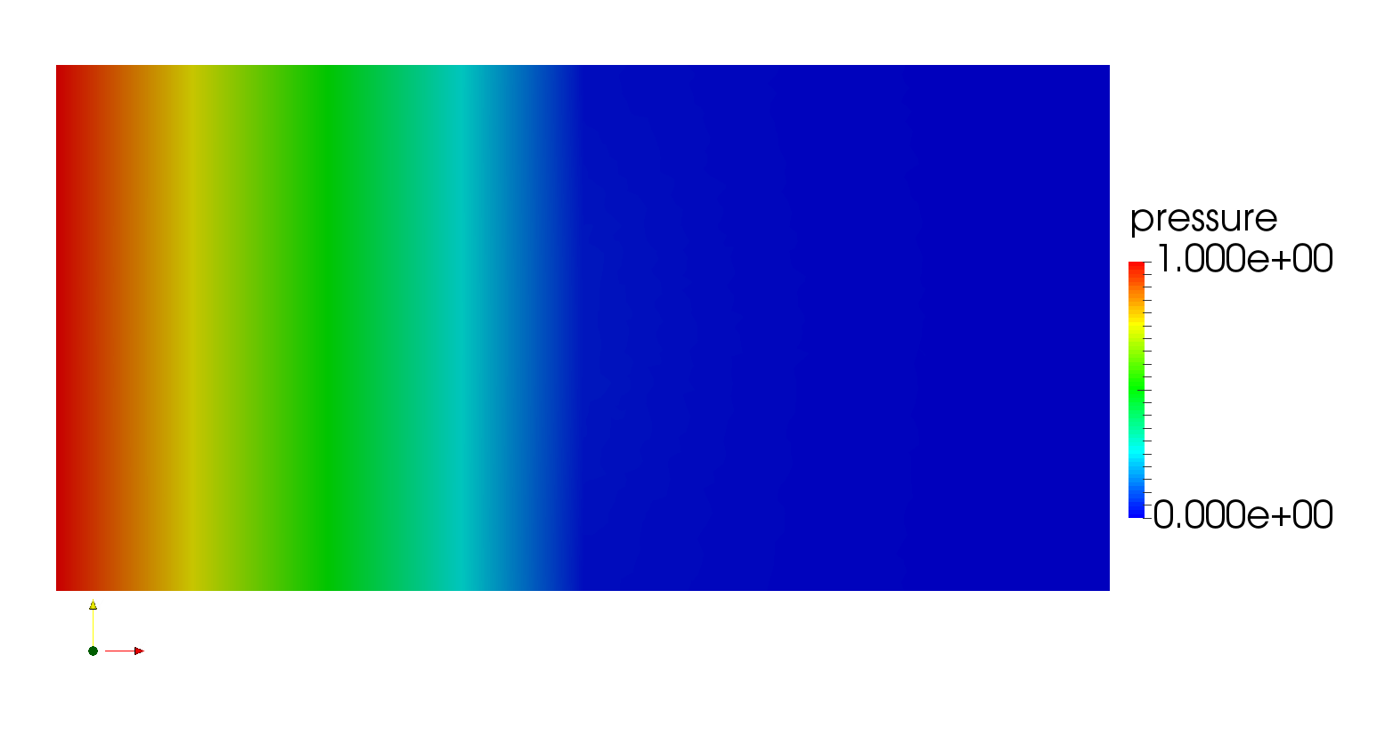
(a) pressure

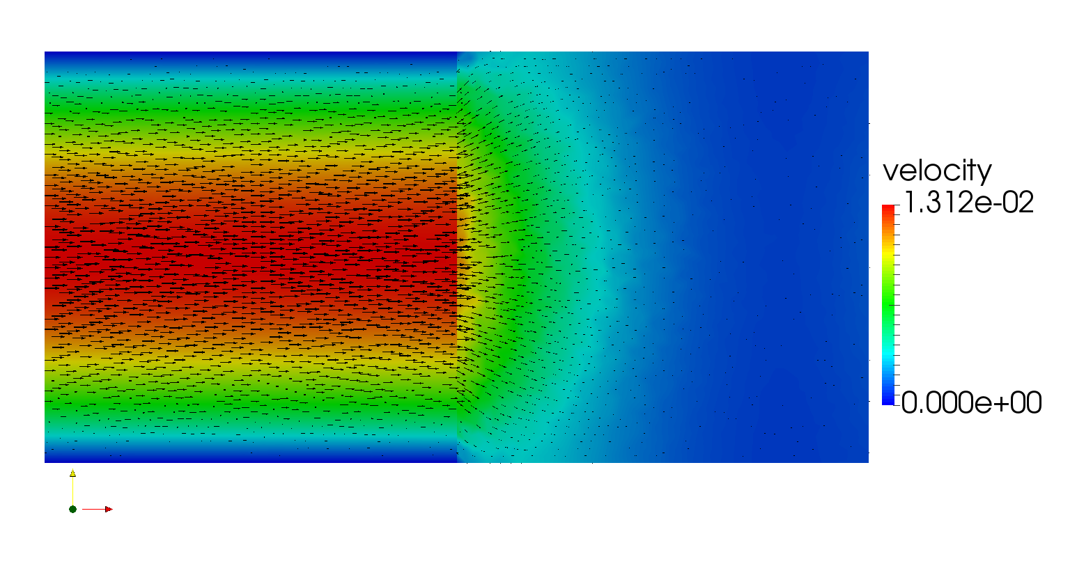
(b) velocity vector (arrows) and magnitude (color)

Figure 1: Example 1, non-Newtonian pressure and velocity solutions at time $t=1$.

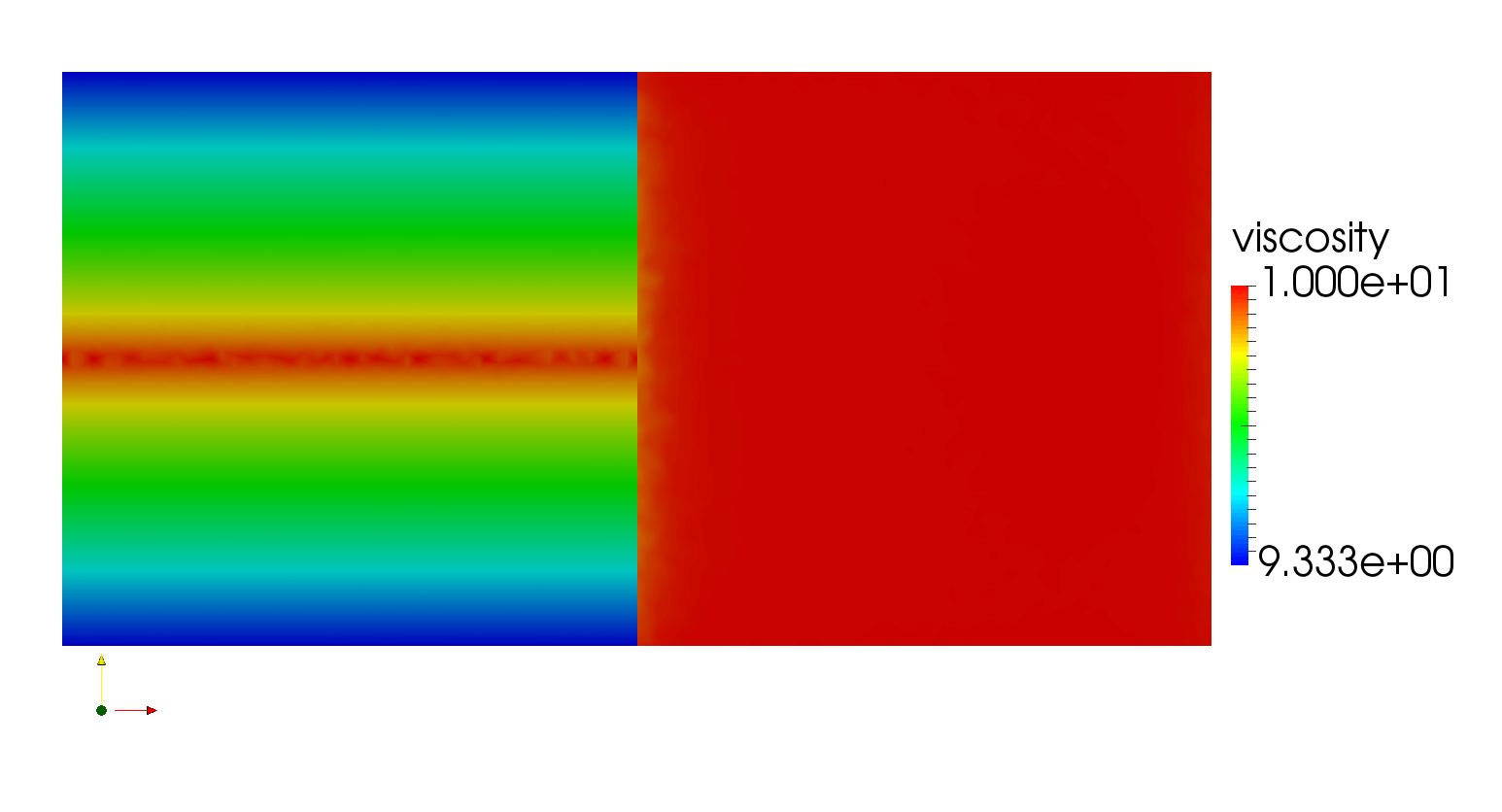
(a) $t=0.01$

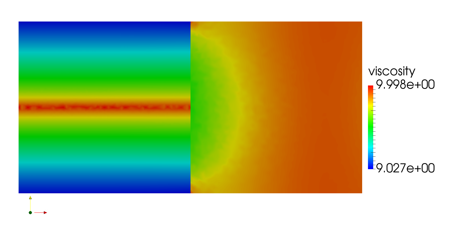
(b) $t=1$

Figure 2: Example 1, nonlinear viscosity.

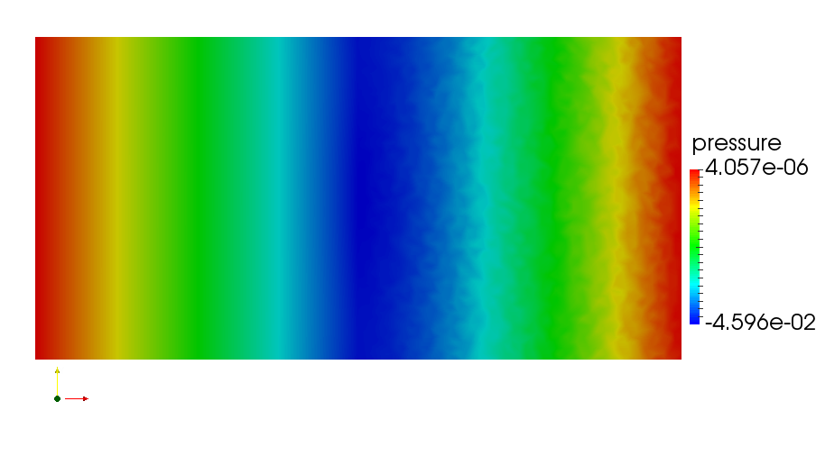
(a) pressure

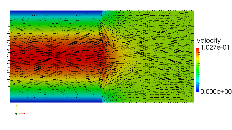
(b) velocity vector (arrows) and magnitude (color)

Figure 3: Example 1, difference between non-Newtonian and Newtonian solutions at time $t=1$.

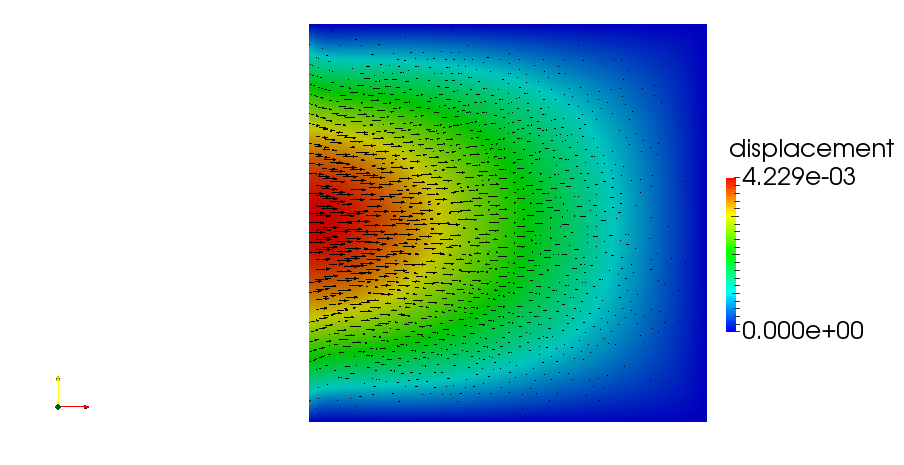
(a) nonlinear displacement

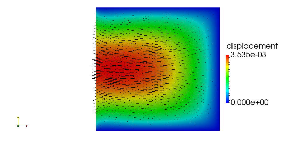
(b) difference

Figure 4: Example 1, non-Newtonian displacement solution and difference at time $t=1$.

7.2 Example 2: application to hydraulic fracturing

We next present an example motivated by hydraulic fracturing. We study the interaction between a stationary fracture filled with fluid and the surrounding reservoir. The units in this example are meters for length, seconds for time, and kPa for pressure. We consider a reference domain $\hat{\Omega}=[0,1]\times[-1,1]$ and a fracture domain $\hat{\Omega}_{f}$, which is located in the middle with a boundary

$$\hat{x}^{2}=200(0.05-\hat{y})(0.05+\hat{y}),\quad\hat{y}\in[-0.05,0.05].$$

The reference poroelastic domain is $\hat{\Omega}_{p}=\hat{\Omega}\setminus\hat{\Omega}_{f}$. The computational domain, shown in Figure 5 (left), is obtained from the reference domain via the mapping

$$\begin{bmatrix}x\\ y\end{bmatrix}(\hat{x},\hat{y})=\begin{bmatrix}x\\ (5\cos(\frac{\hat{x}+\hat{y}}{100})\cos(\frac{\pi\hat{x}+\hat{y}}{100})^{2}+\hat{y}/2-\hat{x}/10)\end{bmatrix}.$$

We enforce an inflow rate ${\bf u}_{f}\cdot{\bf n}_{f}=10$ m/s, ${\bf u}_{f}\cdot\mbox{\boldmath$\tau$}_{f}=0$ m/s on the left part of $\partial\Omega_{f}$ and no flow ${\bf u}_{p}\cdot{\bf n}_{p}=0$ m/s and no stress $\mbox{{\boldmath$\sigma$}}_{p}{\bf n}_{p}={\bf 0}$ kPa on the left part of $\partial\Omega_{p}$. On the top, bottom, and right boundaries we set $p_{p}=1000$ kPa, $\mbox{{\boldmath$\eta$}}_{p}\cdot{\bf n}_{p}=0$ m/s, and $\mbox{{\boldmath$\sigma$}}_{p}{\bf n}_{p}\cdot\mbox{\boldmath$\tau$}_{p}=0$ kPa. The initial conditions are $p_{p}=1000$ kPa and $\mbox{{\boldmath$\eta$}}={\bf 0}$ m/s. The poroelastic parameters, which are typical for hydraulic fracturing and are similar to the ones used in [28], are given in Figure 5 (right). The nonlinear viscosity model in Stokes and Darcy is from [34] for a polymer used in hydraulic fracturing, see Figure 6 (left) for the viscosity dependence on the shear rate. We match the curve using the Cross model (7.1) with parameters $K_{f}=K_{p}=7$, $\nu_{f,\infty}=\nu_{p,\infty}=3.0\times 10^{-6}$ kPa s, $\nu_{f,0}=\nu_{p,0}=1.0\times 10^{-2}$ kPa s, and $r_{f}=r_{p}=1.35$.

We run the simulation for 300 s with time step $\tau=1$ s and compare the results of the linear and nonlinear models. For the linear model we use the viscosity for water, $\nu_{f}^{lin}=\nu_{p}^{lin}=1.0\times 10^{-6}$ kPa s, which is slightly lower than the minimum value of the nonlinear viscosity. We present the simulation results at the final time for both models in Figures 6–8. We note that the scales in the plots are different for the two models, due to significant differences in the solution values. The computed Stokes and Darcy velocities are shown in Figure 7. We observe channel-like flow in the fracture with both models. However, the higher nonlinear viscosity results in smaller velocity, especially near the fracture tip. The nonlinear viscosity in the fracture is shown in Figure 6 (middle). We note the significant shear-thinning effect, especially along the wall of the fracture, where the viscosity is reduced to values in the order of $\nu_{f,\infty}$. Comparing the Darcy velocity fields in Figure 7, we observe that the combination of very small permeability and high fluid viscosity in the nonlinear case results in very little fluid penetration into the reservoir. This is an expected behavior in hydraulic fracturing. Correspondingly, the nonlinear viscosity in the poroelastic region, as shown in Figure 6 (right), is significantly reduced in a close vicinity of the fracture, but is equal to the maximum value $\nu_{p,0}$ away from the fracture. In the linear case, the Darcy velocity is larger and the fluid penetrates further into the reservoir. The behavior for both models is consistent with the computed pressure fields shown in Figure 8. For both models we observe increase in pressure near the fracture. In the linear case the pressure gradient extends away from the fracture. In the nonlinear case, since the fluid cannot penetrate further into the reservoir, we observe a significant pressure buildup along the fracture, about 100 times larger than in the linear case. This in turn results in about 100 times larger displacement in the nonlinear case. This includes larger opening of the fracture, all the way to the tip. We note that our models are for stationary fractures, but the large displacement and corresponding stress near the fracture tip in the nonlinear case may result in practice in fracture propagation, as would be expected in hydraulic fracturing. To summarize, this is a numerically very challenging test case, due to the large stiffness and small permeability of the rock. The numerical difficulty for the non-Newtonian fluid is further increased due to the model nonlinearity and the larger viscosity. We observe that the model is capable of handling parameters in this challenging range and produce results that are qualitatively similar to practical hydraulic fracturing applications.

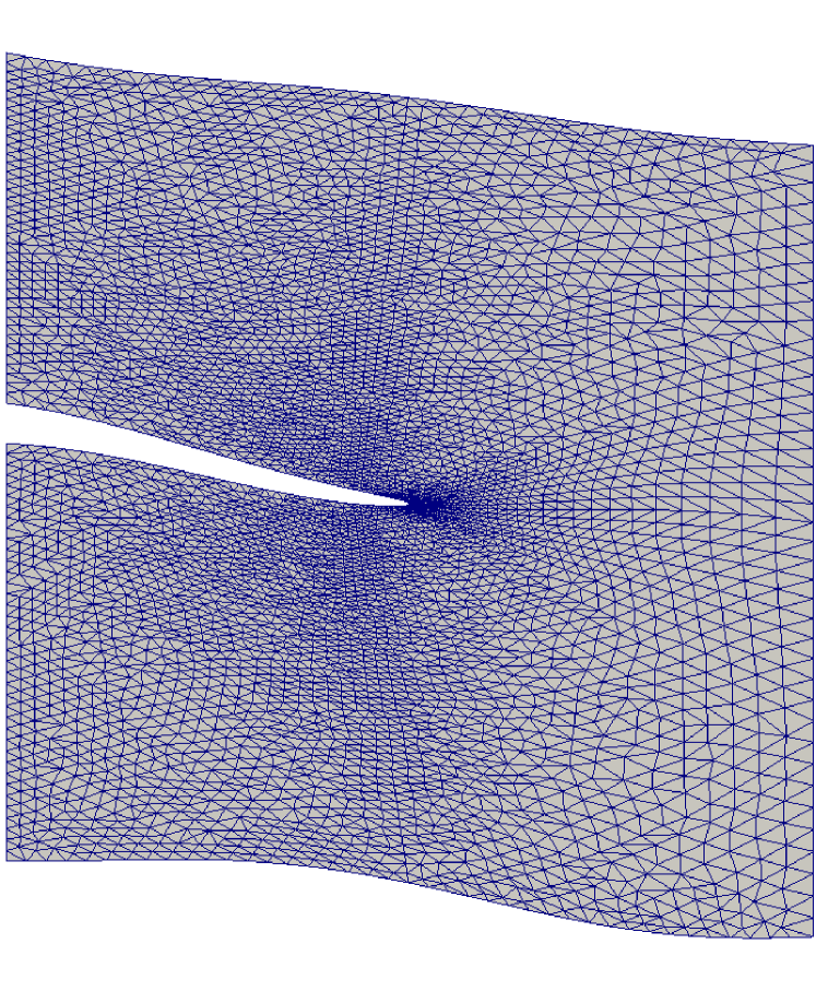
Parameter		Units	Values
Young’s modulus	$E$	(kPa)	$10^{7}$
Poisson’s ratio	$\sigma$		$0.2$
Lame coefficient	$\mu_{p}$	(kPa)	$5/12\times 10^{7}$
Lame coefficient	$\lambda_{p}$	(kPa)	$5/18\times 10^{7}$
Permeability	$K$	(m2)	$(200,50)\times 10^{-12}$
Mass storativity	$s_{0}$	(kPa-1)	$6.89\times 10^{-2}$
Biot-Willis const.	$\alpha$		1.0
BJS coeff.	$\alpha_{BJS}$		1.0
Total time	T	(s)	300

Figure 5: Computational domain (left) and parameters (right) for Example 2.

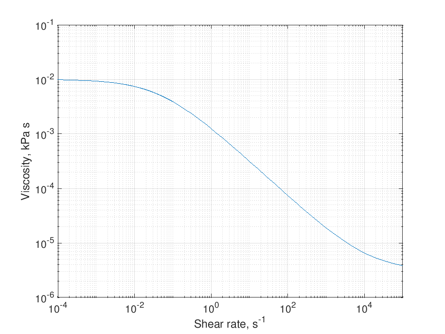
(a) Viscosity model

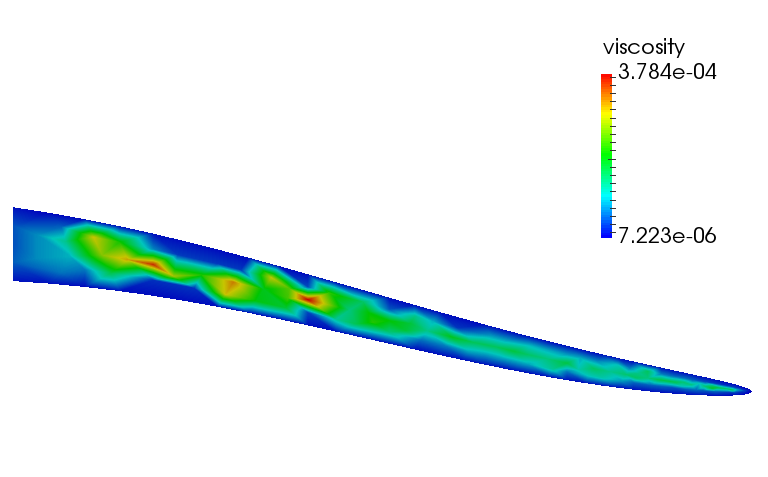
(b) Stokes viscosity

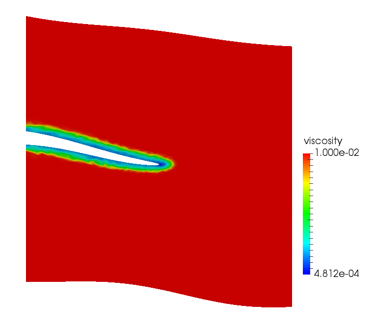
(c) Darcy viscosity

Figure 6: Example 2, nonlinear viscosity model and computed Stokes and Darcy viscosity at $t=300$s.

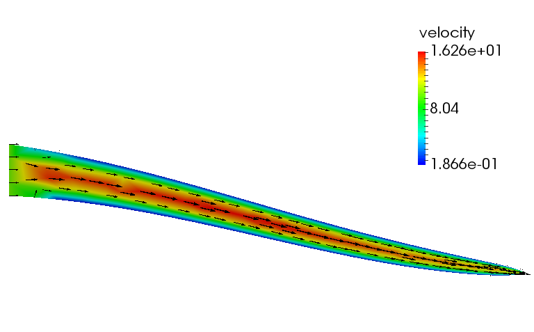
(a) Stokes, linear

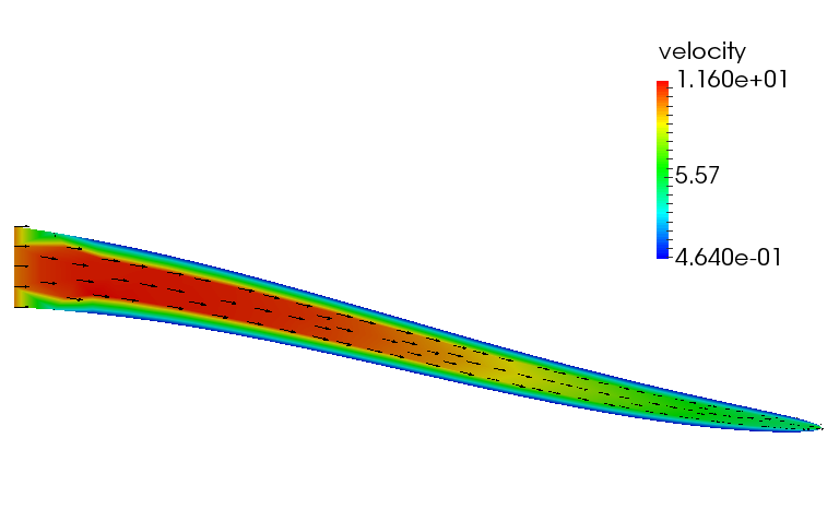
(b) Stokes, nonlinear

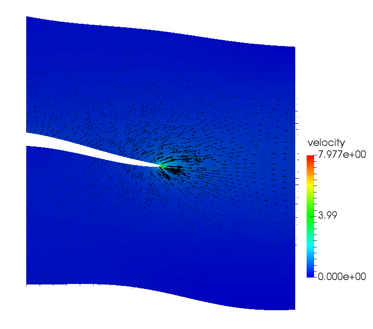
(c) Darcy, linear

(d) Darcy, nonlinear

Figure 7: Example 2, Stokes and Darcy velocity at time $t=300$s.

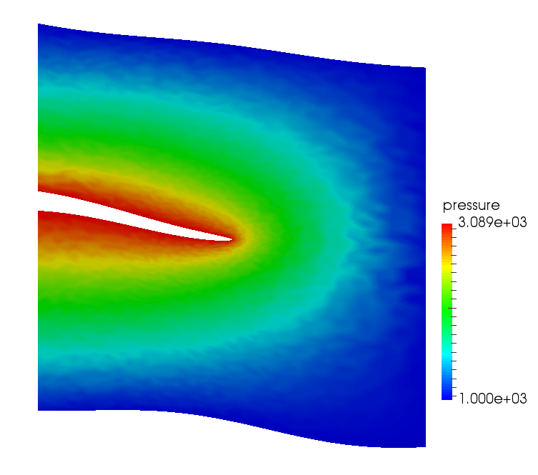
(a) pressure, linear

(b) pressure, nonlinear

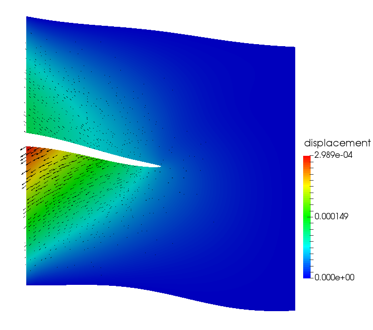
(c) displacement, linear

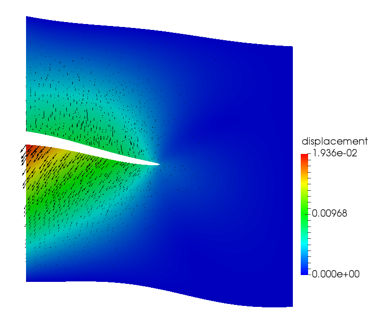
(d) displacement, nonlinear

Figure 8: Example 2, Poroelastic pressure and displacement at time $t=300$s.

References

- [1] G. Acosta, T. Apel, R. Durán, and A. Lombardi. Error estimates for Raviart-Thomas interpolation of any order on anisotropic tetrahedra. Math. Comp., 80(273):141–163, 2011.
- [2] I. Ambartsumyan, E. Khattatov, I. Yotov, and P. Zunino. A Lagrange multiplier method for a Stokes-Biot fluid-poroelastic structure interaction model. Numer. Math., 140(2):513–553, 2018.
- [3] S. Badia, A. Quaini, and A. Quarteroni. Coupling Biot and Navier-Stokes equations for modelling fluid-poroelastic media interaction. J. Comput. Phys., 228(21):7986–8014, 2009.
- [4] G. S. Beavers and D. D. Joseph. Boundary conditions at a naturally impermeable wall. J. Fluid. Mech, 30:197–207, 1967.
- [5] M. Biot. General theory of three-dimensional consolidation. J. Appl. Phys., 12:155–164, 1941.
- [6] R. B. Bird, R. C. Armstrong, O. Hassager, and C. F. Curtiss. Dynamics of polymeric liquids, volume 1. Wiley New York, 1977.
- [7] D. Boffi, F. Brezzi, and M. Fortin. Mixed finite element methods and applications, volume 44 of Springer Series in Computational Mathematics. Springer, Heidelberg, 2013.
- [8] D. Boffi and L. Gastaldi. Analysis of finite element approximation of evolution problems in mixed form. SIAM J. Numer. Anal., 42(4):1502–1526, 2004.
- [9] F. Brezzi, D. Boffi, L. Demkowicz, R. G. Durán, R. S. Falk, and M. Fortin. Mixed finite elements, compatibility conditions, and applications. Springer, 2008.
- [10] M. Bukac, I. Yotov, R. Zakerzadeh, and P. Zunino. Partitioning strategies for the interaction of a fluid with a poroelastic material based on a Nitsche’s coupling approach. Comput. Methods Appl. Mech. Engrg., 292:138–170, 2015.
- [11] M. Bukac, I. Yotov, and P. Zunino. An operator splitting approach for the interaction between a fluid and a multilayered poroelastic structure. Numer. Methods Partial Differential Equations, 31(4):1054–1100, 2015.
- [12] M. Bukac, I. Yotov, and P. Zunino. Dimensional model reduction for flow through fractures in poroelastic media. ESAIM Math. Model. Numer. Anal., 51(4):1429–1471, 2017.
- [13] S. Caucao, G. N. Gatica, R. Oyarzúa, and I. Sebestová. A fully-mixed finite element method for the Navier-Stokes/Darcy coupled problem with nonlinear viscosity. J. Numer. Math., 25(2):55–88, 2017.
- [14] A. Cesmelioglu. Analysis of the coupled Navier-Stokes/Biot problem. J. Math. Anal. Appl., 456(2):970–991, 2017.
- [15] A. Cesmelioglu, H. Lee, A. Quaini, K. Wang, and S.-Y. Yi. Optimization-based decoupling algorithms for a fluid-poroelastic system. In Topics in numerical partial differential equations and scientific computing, volume 160 of IMA Vol. Math. Appl., pages 79–98. Springer, New York, 2016.
- [16] S.-S. Chow and G. F. Carey. Numerical approximation of generalized Newtonian fluids using Powell–Sabin–Heindl elements: I. Theoretical estimates. Internat. J. Numer. Methods Fluids, 41(10):1085–1118, 2003.
- [17] M. Dauge. Elliptic boundary value problems on corner domains, volume 1341 of Lecture Notes in Mathematics. Springer-Verlag, Berlin, 1988. Smoothness and asymptotics of solutions.
- [18] D. Di Pietro and J. Droniou. A hybrid high-order method for Leray–Lions elliptic equations on general meshes. Math. Comp., 86(307):2159–2191, 2017.
- [19] M. Discacciati, E. Miglio, and A. Quarteroni. Mathematical and numerical models for coupling surface and groundwater flows. Appl. Numer. Math., 43(1-2):57–74, 2002.
- [20] S. Domínguez, G. N. Gatica, A. Márquez, and S. Meddahi. A primal-mixed formulation for the strong coupling of quasi-Newtonian fluids with porous media. Adv. Comput. Math., 42(3):675–720, 2016.
- [21] R. Durán. Error analysis in , for mixed finite element methods for linear and quasi-linear elliptic problems. ESAIM: Math. Model. Numer. Anal., 22(3):371–387, 1988.
- [22] V. J. Ervin, E. W. Jenkins, and S. Sun. Coupled generalized nonlinear Stokes flow with flow through a porous medium. SIAM J. Numer. Anal., 47(2):929–952, 2009.
- [23] V. J. Ervin, E. W. Jenkins, and S. Sun. Coupling nonlinear Stokes and Darcy flow using mortar finite elements. Appl. Numer. Math., 61(11):1198–1222, 2011.
- [24] L. Formaggia, A. Quarteroni, and A. Veneziani. Cardiovascular Mathematics: Modeling and simulation of the circulatory system, volume 1. Springer Science & Business Media, 2010.
- [25] S. Frei, B. Holm, T. Richter, T. Wick, and H. Yang, editors. Fluid-Structure Interaction: Modeling, Adaptive Discretisations and Solvers, volume 20 of Radon Series on Computational and Applied Mathematics. De Gruyter, 2017.
- [26] G. P. Galdi. An introduction to the mathematical theory of the Navier-Stokes equations: Steady-state problems. Springer Science & Business Media, 2011.
- [27] G. P. Galdi and R. Rannacher, editors. Fundamental trends in fluid-structure interaction, volume 1 of Contemporary Challenges in Mathematical Fluid Dynamics and Its Applications. World Scientific Publishing Co. Pte. Ltd., Hackensack, NJ, 2010.
- [28] V. Girault, M. F. Wheeler, B. Ganis, and M. E. Mear. A lubrication fracture model in a poro-elastic medium. Math. Models Methods Appl. Sci., 25(4):587–645, 2015.
- [29] P. Grisvard. Elliptic problems in nonsmooth domains. SIAM, 2011.
- [30] F. Hecht. New development in FreeFem++. J. Numer. Math., 20(3-4):251–265, 2012.
- [31] J. Janela, A. Moura, and A. Sequeira. A 3D non-Newtonian fluid–structure interaction model for blood flow in arteries. J. Comput. Appl. Math., 234(9):2783–2791, 2010.
- [32] W. J. Layton, F. Schieweck, and I. Yotov. Coupling fluid flow with porous media flow. SIAM J. Numer. Anal., 40(6):2195–2218, 2003.
- [33] S. Lee, A. Mikelić, M. F. Wheeler, and T. Wick. Phase-field modeling of proppant-filled fractures in a poroelastic medium. Comput. Methods Appl. Mech. Engrg., 312:509–541, 2016.
- [34] X. Lopez, P. H. Valvatne, and M. J. Blunt. Predictive network modeling of single-phase non-Newtonian flow in porous media. J. Colloid Interface Sci., 264(1):256–265, 2003.
- [35] J. Necas, J. Málek, M. Rokyta, and M. Ruzicka. Weak and measure-valued solutions to evolutionary PDEs, volume 13. CRC Press, 1996.
- [36] R. G. Owens and T. N. Phillips. Computational rheology, volume 14. World Scientific, 2002.
- [37] J. R. A. Pearson and P. M. J. Tardy. Models for flow of non-Newtonian and complex fluids through porous media. J. non-Newton. fluid mech., 102(2):447–473, 2002.
- [38] M. Renardy and R. C. Rogers. An introduction to partial differential equations, volume 13. Springer Science & Business Media, 2006.
- [39] B. Rivière and I. Yotov. Locally conservative coupling of Stokes and Darcy flows. SIAM J. Numer. Anal., 42(5):1959–1977, 2005.
- [40] P. G. Saffman. On the boundary condition at the surface of a porous media. Stud. Appl. Math., 50:93–101, 1971.
- [41] D. Sandri. Sur l’approximation numérique des écoulements quasi-newtoniens dont la viscosité suit la loi puissance ou la loi de Carreau. RAIRO Modél. Math. Anal. Numér., 27(2):131–155, 1993.
- [42] L. R. Scott and S. Zhang. Finite element interpolation of nonsmooth functions satisfying boundary conditions. Math. Comp., 54, 1990.
- [43] R. E. Showalter. Poroelastic filtration coupled to Stokes flow. In Control theory of partial differential equations, volume 242 of Lect. Notes Pure Appl. Math., pages 229–241. Chapman & Hall/CRC, Boca Raton, FL, 2005.
- [44] R. E. Showalter. Nonlinear degenerate evolution equations in mixed formulation. SIAM J. Math. Anal., 42(5):2114–2131, 2010.
- [45] R. E. Showalter. Monotone operators in Banach space and nonlinear partial differential equations, volume 49. American Mathematical Soc., 2013.