Abstract

Deep neural network training spends most of the computation on examples that are properly handled, and could be ignored.

We propose to mitigate this phenomenon with a principled importance sampling scheme that focuses computation on “informative” examples, and reduces the variance of the stochastic gradients during training. Our contribution is twofold: first, we derive a tractable upper bound to the per-sample gradient norm, and second we derive an estimator of the variance reduction achieved with importance sampling, which enables us to switch it on when it will result in an actual speedup.

The resulting scheme can be used by changing a few lines of code in a standard SGD procedure, and we demonstrate experimentally, on image classification, CNN fine-tuning, and RNN training, that for a fixed wall-clock time budget, it provides a reduction of the train losses of up to an order of magnitude and a relative improvement of test errors between 5% and 17%.

1 Introduction

The dramatic increase in available training data has made the use of deep neural networks feasible, which in turn has significantly improved the state-of-the-art in many fields, in particular computer vision and natural language processing. However, due to the complexity of the resulting optimization problem, computational cost is now the core issue in training these large architectures.

When training such models, it appears to any practitioner that not all samples are equally important; many of them are properly handled after a few epochs of training, and most could be ignored at that point without impacting the final model. To this end, we propose a novel importance sampling scheme that accelerates the training of any neural network architecture by focusing the computation on the samples that will introduce the biggest change in the parameters which reduces the variance of the gradient estimates.

For convex optimization problems, many works Bordes et al. (2005); Zhao & Zhang (2015); Needell et al. (2014); Canévet et al. (2016); Richtárik & Takáč (2013) have taken advantage of the difference in importance among the samples to improve the convergence speed of stochastic optimization methods. On the other hand, for deep neural networks, sample selection methods were mainly employed to generate hard negative samples for embedding learning problems or to tackle the class imbalance problem Schroff et al. (2015); Wu et al. (2017); Simo-Serra et al. (2015).

Recently, researchers have shifted their focus on using importance sampling to improve and accelerate the training of neural networks Alain et al. (2015); Loshchilov & Hutter (2015); Schaul et al. (2015). Those works, employ either the gradient norm or the loss to compute each sample’s importance. However, the former is prohibitively expensive to compute and the latter is not a particularly good approximation of the gradient norm.

Compared to the aforementioned works, we derive an upper bound to the per sample gradient norm that can be computed in a single forward pass. This results in reduced computational requirements of more than an order of magnitude compared to Alain et al. (2015). Furthermore, we quantify the variance reduction achieved with the proposed importance sampling scheme and associate it with the batch size increment required to achieve an equivalent variance reduction. The benefits of this are twofold, firstly we provide an intuitive metric to predict how useful importance sampling is going to be, thus we are able to decide when to switch on importance sampling during training. Secondly, we also provide theoretical guarantees for speedup, when variance reduction is above a threshold. Based on our analysis, we propose a simple to use algorithm that can be used to accelerate the training of any neural network architecture.

Our implementation is generic and can be employed by adding a single line of code in a standard Keras model training. We validate it on three independent tasks: image classification, fine-tuning and sequence classification with recurrent neural networks. Compared to existing batch selection schemes, we show that our method consistently achieves lower training loss and test error for equalized wall-clock time.

2 Related Work

Existing importance sampling methods can be roughly categorized in methods applied to convex problems and methods designed for deep neural networks.

2.1 Importance Sampling for Convex Problems

Importance sampling for convex optimization problems has been extensively studied over the last years. Bordes et al. (2005) developed LASVM, which is an online algorithm that uses importance sampling to train kernelized support vector machines. Later, Richtárik & Takáč (2013) proposed a generalized coordinate descent algorithm that samples coordinate sets in a way that optimizes the algorithm’s convergence rate.

More recent works Zhao & Zhang (2015); Needell et al. (2014) make a clear connection with the variance of the gradient estimates of stochastic gradient descent and show that the optimal sampling distribution is proportional to the per sample gradient norm. Due to the relatively simple optimization problems that they deal with, the authors resort to sampling proportionally to the norm of the inputs, which in simple linear classification is proportional to the Lipschitz constant of the per sample loss function.

Such simple importance measures do not exist for Deep Learning and the direct application of the aforementioned theory Alain et al. (2015), requires clusters of GPU workers just to compute the sampling distribution.

2.2 Importance Sampling for Deep Learning

Importance sampling has been used in Deep Learning mainly in the form of manually tuned sampling schemes. Bengio et al. (2009) manually design a sampling scheme inspired by the perceived way that human children learn; in practice they provide the network with examples of increasing difficulty in an arbitrary manner. Diametrically opposite, it is common for deep embedding learning to sample hard examples because of the plethora of easy non informative ones Simo-Serra et al. (2015); Schroff et al. (2015).

More closely related to our work, Schaul et al. (2015) and Loshchilov & Hutter (2015) use the loss to create the sampling distribution. Both approaches keep a history of losses for previously seen samples, and sample either proportionally to the loss or based on the loss ranking. One of the main limitations of history based sampling, is the need for tuning a large number of hyperparameters that control the effects of “stale” importance scores; i.e. since the model is constantly updated, the importance of samples fluctuate and previous observations may poorly reflect the current situation. In particular, Schaul et al. (2015) use various forms of smoothing for the losses and the importance sampling weights, while Loshchilov & Hutter (2015) introduce a large number of hyperparameters that control when the losses are computed, when they are sorted as well as how the sampling distribution is computed based on the rank.

In comparison to all the above methods, our importance sampling scheme based on an upper bound to the gradient norm has a solid theoretical basis with clear objectives, very easy to choose hyperparameters, theoretically guaranteed speedup and can be applied to any type of network and loss function.

2.3 Other Sample Selection Methods

For completeness, we mention the work of Wu et al. (2017), who design a distribution (suitable only for the distance based losses) that maximizes the diversity of the losses in a single batch. In addition, Fan et al. (2017) use reinforcement learning to train a neural network that selects samples for another neural network in order to optimize the convergence speed. Although their preliminary results are promising, the overhead of training two networks makes the wall-clock speedup unlikely and their proposal not as appealing.

2.4 Stochastic Variance Reduced Gradient

Finally, a class of algorithms that aim to accelerate the convergence of Stochastic Gradient Descent (SGD) through variance reduction are SVRG type algorithms Johnson & Zhang (2013); Defazio et al. (2014); Allen-Zhu (2017); Lei et al. (2017). Although asymptotically better, those algorithms typically perform worse than plain SGD with momentum for the low accuracy optimization setting of Deep Learning. Contrary to the aforementioned algorithms, our proposed importance sampling does not improve the asymptotic convergence of SGD but results in pragmatic improvements in all the metrics given a fixed time budget.

3 Variance Reduction for Deep Neural Networks

Importance sampling aims at increasing the convergence speed of SGD by focusing computation on samples that actually induce a change in the model parameters. This formally translates into a reduced variance of the gradient estimates for a fixed computational cost. In the following sections, we analyze how this works and present an efficient algorithm that can be used to train any Deep Learning model.

3.1 Introduction to Importance Sampling

Let $x_{i}$, $y_{i}$ be the $i$-th input-output pair from the training set, $\Psi(\cdot;\theta)$ be a Deep Learning model parameterized by the vector $\theta$, and $\mathcal{L}(\cdot,\cdot)$ be the loss function to be minimized during training. The goal of training is to find

$$\theta^{*}=\operatorname*{arg\,min}_{\theta}\frac{1}{N}\sum_{i=1}^{N}\mathcal{L}(\Psi(x_{i};\theta),y_{i})$$ (1)

where $N$ corresponds to the number of examples in the training set.

We use an SGD procedure with learning rate $\eta$, where the update at iteration $t$ depends on the sampling distribution $p^{t}_{1},\dots,p^{t}_{N}$ and re-scaling coefficients $w^{t}_{1},\dots,w^{t}_{N}$. Let $I_{t}$ be the data point sampled at that step, we have $P(I_{t}=i)=p^{t}_{i}$ and

$$\theta_{t+1}=\theta_{t}-\eta w_{I_{t}}\nabla_{\theta_{t}}\mathcal{L}(\Psi(x_{I_{t}};\theta_{t}),y_{I_{t}})$$ (2)

Plain SGD with uniform sampling is achieved with $w^{t}_{i}=1$ and $p^{t}_{i}=\frac{1}{N}$ for all $t$ and $i$.

If we define the convergence speed $S$ of SGD as the reduction of the distance of the parameter vector $\theta$ from the optimal parameter vector $\theta^{*}$ in two consecutive iterations $t$ and $t+1$

$$S=-\operatorname{\mathbb{E}}_{P_{t}}\!\left[\left\lVert\theta_{t+1}-\theta^{*}\right\rVert_{2}^{2}-\left\lVert\theta_{t}-\theta^{*}\right\rVert_{2}^{2}\right],$$ (3)

and if we have $w_{i}=\frac{1}{Np_{i}}$ such that

$$\operatorname{\mathbb{E}}_{P_{t}}\!\left[w_{I_{t}}\nabla_{\theta_{t}}\mathcal{L}(\Psi(x_{I_{t}};\theta_{t}),y_{I_{t}})\right]$$ (4)

$$\quad=\nabla_{\theta_{t}}\frac{1}{N}\sum_{i=1}^{N}\mathcal{L}(\Psi(x_{i};\theta_{t}),y_{i}),$$ (5)

and set $G_{i}=w_{i}\nabla_{\theta_{t}}\mathcal{L}(\Psi(x_{i};\theta_{t}),y_{i})$, then we get (this is a different derivation of the result by Wang et al., 2016)

$$S =-\operatorname{\mathbb{E}}_{P_{t}}\!\left[\left(\theta_{t+1}\!-\!\theta^{*}\right)^{T}\!\left(\theta_{t+1}\!-\!\theta^{*}\right)-\left(\theta_{t}\!-\!\theta^{*}\right)^{T}\!\left(\theta_{t}\!-\!\theta^{*}\right)\right]$$ (6)

$$=-\operatorname{\mathbb{E}}_{P_{t}}\!\left[\theta_{t+1}^{T}\!\theta_{t+1}\!-\!2\theta_{t+1}\theta^{*}-\theta_{t}^{T}\!\theta_{t}+2\theta_{t}\theta^{*}\right]$$

$$=-\operatorname{\mathbb{E}}_{P_{t}}\!\left[\left(\theta_{t}\!-\!\eta G_{I_{t}}\right)^{T}\!\left(\theta_{t}\!-\!\eta G_{I_{t}}\right)+2\eta G_{I_{t}}^{T}\!\theta^{*}\!-\!\theta_{t}^{T}\!\theta_{t}\right]$$

$$=-\operatorname{\mathbb{E}}_{P_{t}}\!\left[-2\eta\left(\theta_{t}\!-\!\theta^{*}\right)G_{I_{t}}+\eta^{2}G_{I_{t}}^{T}\!G_{I_{t}}\right]$$

$$=2\eta\left(\theta_{t}\!-\!\theta^{*}\right)\operatorname{\mathbb{E}}_{P_{t}}\!\left[G_{I_{t}}\right]-\eta^{2}\operatorname{\mathbb{E}}_{P_{t}}\!\left[G_{I_{t}}\right]^{T}\!\operatorname{\mathbb{E}}_{P_{t}}\!\left[G_{I_{t}}\right]-$$

$$\quad\,\eta^{2}\text{Tr}\left(\operatorname{\mathbb{V}}_{P_{t}}\!\left[G_{I_{t}}\right]\right)$$

Since the first two terms, in the last expression, are the speed of batch gradient descent, we observe that it is possible to gain a speedup by sampling from the distribution that minimizes $\text{Tr}\left(\operatorname{\mathbb{V}}_{P_{t}}\!\left[G_{I_{t}}\right]\right)$. Several works Needell et al. (2014); Zhao & Zhang (2015); Alain et al. (2015) have shown the optimal distribution to be proportional to the per-sample gradient norm. However, computing this distribution is computationally prohibitive.

3.2 Beyond the Full Gradient Norm

Given an upper bound $\hat{G}_{i}\geq\left\lVert\nabla_{\theta_{t}}\mathcal{L}(\Psi(x_{i};\theta_{t}),y_{i})\right\rVert_{2}$ and due to

$$\operatorname*{arg\,min}_{P}\text{Tr}\left(\operatorname{\mathbb{V}}_{P_{t}}\!\left[G_{I_{t}}\right]\right)=\operatorname*{arg\,min}_{P}\operatorname{\mathbb{E}}_{P_{t}}\!\left[\left\lVert G_{I_{t}}\right\rVert_{2}^{2}\right],$$ (7)

we propose to relax the optimization problem in the following way

$$\min_{P}\operatorname{\mathbb{E}}_{P_{t}}\!\left[\left\lVert G_{I_{t}}\right\rVert_{2}^{2}\right]\leq\min_{P}\operatorname{\mathbb{E}}_{P_{t}}\!\left[w_{I_{t}}^{2}\hat{G}_{I_{t}}^{2}\right].$$ (8)

The minimizer of the second term of equation 8, similar to the first term, is $p_{i}\propto\hat{G}_{i}$. All that remains, is to find a proper expression for $\hat{G}_{i}$ which is significantly easier to compute than the norm of the gradient for each sample.

In order to continue with the derivation of our upper bound $\hat{G}_{i}$, let us introduce some notation specific to a multi-layer perceptron. Let $\theta^{(l)}\in\mathbb{R}^{M_{l}\times M_{l-1}}$ be the weight matrix for layer $l$ and $\sigma^{(l)}(\cdot)$ be a Lipschitz continuous activation function. Then, let

$$x^{(0)} =x$$ (9)

$$z^{(l)} =\theta^{(l)}\,x^{(l-1)}$$ (10)

$$x^{(l)} =\sigma^{(l)}(z^{(l)})$$ (11)

$$\Psi(x;\Theta) =x^{(L)}$$ (12)

Although our notation describes simple fully connected neural networks without bias, our analysis holds for any affine operation followed by a slope-bounded non-linearity ($|\sigma^{\prime}(x)|\leq K$). With

$$\Sigma_{l}^{\prime}(z) =diag\left(\sigma^{\prime(l)}(z_{1}),\dots,\sigma^{\prime(l)}(z_{M_{l}})\right),$$ (13)

$$\Delta_{i}^{(l)} =\Sigma_{l}^{\prime}(z_{i}^{(l)})\theta_{l+1}^{T}\dots\Sigma_{L-1}^{\prime}(z_{i}^{(L-1)})\theta_{L}^{T},$$ (14)

$$\nabla_{x_{i}^{(L)}}\mathcal{L} =\nabla_{x_{i}^{(L)}}\mathcal{L}(\Psi(x_{i};\Theta),y_{i})$$ (15)

we get

$$\left\lVert\nabla_{\theta_{l}}\mathcal{L}(\Psi(x_{i};\Theta),y_{i})\right\rVert_{2}$$ (16)

$$= \left\lVert\left(\Delta_{i}^{(l)}\Sigma_{L}^{\prime}(z_{i}^{(L)})\nabla_{x_{i}^{(L)}}\mathcal{L}\right)\left(x_{i}^{(l-1)}\right)^{T}\right\rVert_{2}$$ (17)

$$\leq \left\lVert\Delta_{i}^{(l)}\right\rVert_{2}\left\lVert\Sigma_{L}^{\prime}(z_{i}^{(L)})\nabla_{x_{i}^{(L)}}\mathcal{L}\right\rVert_{2}\left\lVert x_{i}^{(l-1)}\right\rVert_{2}$$ (18)

$$\leq \underbrace{\max_{l,i}\left(\left\lVert x_{i}^{(l-1)}\right\rVert_{2}\left\lVert\Delta_{i}^{(l)}\right\rVert_{2}\right)}_{\rho}\left\lVert\Sigma_{L}^{\prime}(z_{i}^{(L)})\nabla_{x_{i}^{(L)}}\mathcal{L}\right\rVert_{2}$$ (19)

Various weight initialization Glorot & Bengio (2010) and activation normalization techniques Ioffe & Szegedy (2015); Ba et al. (2016) uniformise the activations across samples. As a result, the variation of the gradient norm is mostly captured by the gradient of the loss function with respect to the pre-activation outputs of the last layer of our neural network. Consequently we can derive the following upper bound to the gradient norm of all the parameters

$$\left\lVert\nabla_{\Theta}\mathcal{L}(\Psi(x_{i};\Theta),y_{i})\right\rVert_{2}\leq\underbrace{L\rho\left\lVert\Sigma_{L}^{\prime}(z_{i}^{(L)})\nabla_{x_{i}^{(L)}}\mathcal{L}\right\rVert_{2}}_{\hat{G}_{i}},$$ (20)

which is marginally more difficult to compute than the value of the loss since it can be computed in a closed form in terms of $z^{(L)}$. However, our upper bound depends on the time step $t$, thus we cannot generate a distribution once and sample from it during training. This is intuitive because the importance of each sample changes as the model changes.

3.3 When is Variance Reduction Possible?

Computing the importance score from equation 20 is more than an order of magnitude faster compared to computing the gradient norm for each sample. Nevertheless, it still costs one forward pass through the network and can be wasteful. For instance, during the first iterations of training, the gradients with respect to every sample have approximately equal norm; thus we would waste computational resources trying to sample from the uniform distribution. In addition, computing the importance score for the whole dataset is still prohibitive and would render the method unsuitable for online learning.

In order to solve the problem of computing the importance for the whole dataset, we pre-sample a large batch of data points, compute the sampling distribution for that batch and re-sample a smaller batch with replacement. The above procedure upper bounds both the speedup and variance reduction. Given a large batch consisting of $B$ samples and a small one consisting of $b$, we can achieve a maximum variance reduction of $\frac{1}{b}-\frac{1}{B}$ and a maximum speedup of $\frac{B+3b}{3B}$ assuming that the backward pass requires twice the amount of time as the forward pass.

Due to the large cost of computing the importance per sample, we only perform importance sampling when we know that the variance of the gradients can be reduced. In the following equation, we show that the variance reduction is proportional to the squared $L_{2}$ distance of the sampling distribution, $g$, to the uniform distribution $u$. Due to lack of space, the complete derivation is included in the supplementary material. Let $g_{i}\propto\left\lVert\nabla_{\theta_{t}}\mathcal{L}(\Psi(x_{i};\theta_{t}),y_{i})\right\rVert_{2}=\left\lVert G_{i}\right\rVert_{2}$ and $u=\frac{1}{B}$ the uniform probability.

$$\text{Tr}\left(\operatorname{\mathbb{V}}_{u}\!\left[G_{i}\right]\right)-\text{Tr}\left(\operatorname{\mathbb{V}}_{g}\!\left[w_{i}G_{i}\right]\right)$$ (21)

$$=\operatorname{\mathbb{E}}_{u}\!\left[\left\lVert G_{i}\right\rVert_{2}^{2}\right]-\operatorname{\mathbb{E}}_{g}\!\left[w_{i}^{2}\left\lVert G_{i}\right\rVert_{2}^{2}\right]$$ (22)

$$=\left(\frac{1}{B}\sum_{i=1}^{B}\left\lVert G_{i}\right\rVert_{2}\right)^{2}B\left\lVert g-u\right\rVert_{2}^{2}.$$ (23)

Equation 23 already provides us with a useful metric to decide if the variance reduction is significant enough to justify using importance sampling. However, choosing a suitable threshold for the $L_{2}$ distance squared would be tedious and unintuitive. We can do much better by dividing the variance reduction with the original variance to derive the increase in the batch size that would achieve an equivalent variance reduction. Assuming that we increase the batch size by $\tau$, we achieve variance reduction $\frac{1}{\tau}$; thus we have

$$\frac{\left(\frac{1}{B}\sum_{i=1}^{B}\left\lVert G_{i}\right\rVert_{2}\right)^{2}B\left\lVert g-u\right\rVert_{2}^{2}}{\text{Tr}\left(\operatorname{\mathbb{V}}_{u}\!\left[G_{i}\right]\right)}\geq$$ (24)

$$\frac{\left(\frac{1}{B}\sum_{i=1}^{B}\left\lVert G_{i}\right\rVert_{2}\right)^{2}B\left\lVert g-u\right\rVert_{2}^{2}}{\frac{1}{B}\sum_{i=1}^{B}\left\lVert G_{i}\right\rVert_{2}^{2}}=$$ (25)

$$\frac{1}{\sum_{i=1}^{B}g_{i}^{2}}\left\lVert g-u\right\rVert_{2}^{2}=1-\frac{1}{\tau}\iff$$ (26)

$$\frac{1}{\tau}=1-\frac{1}{\sum_{i=1}^{B}g_{i}^{2}}\left\lVert g-u\right\rVert_{2}^{2}$$ (27)

Using equation 27, we have a hyperparameter that is very easy to select and can now design our training procedure which is described in pseudocode in algorithm 1. Computing $\tau$ from equation 27 allows us to have guaranteed speedup when $B+3b<3\tau b$. However, as it is shown in the experiments, we can use $\tau_{th}$ smaller than $\frac{B+3b}{3b}$ and still get a significant speedup.

Algorithm 1 Deep Learning with Importance Sampling

1:  Inputs $B,b,\tau_{th},a_{\tau},\theta_{0}$

2:  $t\leftarrow 1$

3:  $\tau\leftarrow 0$

4:  repeat

5:     if $\tau>\tau_{th}$ then

6:        $\mathcal{U}\leftarrow B$ uniformly sampled datapoints

7:        $g_{i}\propto\hat{G_{i}}\quad\forall i\in\mathcal{U}$ according to eq 20

8:        $\mathcal{G}\leftarrow b$ datapoints sampled with $g_{i}$ from $\mathcal{U}$

9:        $w_{i}\leftarrow\frac{1}{Bg_{i}}\quad\forall i\in\mathcal{G}$

10:        $\theta_{t}\leftarrow\text{sgd\_step}(w_{i},\mathcal{G},\theta_{t-1})$

11:     else

12:        $\mathcal{U}\leftarrow b$ uniformly sampled datapoints

13:        $w_{i}\leftarrow 1\quad\forall i\in\mathcal{U}$

14:        $\theta_{t}\leftarrow\text{sgd\_step}(w_{i},\mathcal{U},\theta_{t-1})$

15:        $g_{i}\propto\hat{G_{i}}\quad\forall i\in\mathcal{U}$

16:     end if

17:     $\tau\leftarrow a_{\tau}\tau+(1-a_{\tau})\left(1-\frac{1}{\sum_{i}g_{i}^{2}}\left\lVert g-\frac{1}{|\mathcal{U}|}\right\rVert_{2}^{2}\right)^{-1}$

18:  until convergence

The inputs to the algorithm are the pre-sampling size $B$, the batch size $b$, the equivalent batch size increment after which we start importance sampling $\tau_{th}$ and the exponential moving average parameter $a_{\tau}$ used to compute a smooth estimate of $\tau$. $\theta_{0}$ denotes the initial parameters of our deep network. We would like to point out that in line 15 of the algorithm, we compute $g_{i}$ for free since we have done the forward pass in the previous step.

The only parameter that has to be explicitly defined for our algorithm is the pre-sampling size $B$ because $\tau_{th}$ can be set using equation 27. We provide a small ablation study for $B$ in the supplementary material.

4 Experiments

In this section, we analyse experimentally the performance of the proposed importance sampling scheme based on our upper-bound of the gradient norm. In the first subsection, we compare the variance reduction achieved with our upper bound to the theoretically maximum achieved with the true gradient norm. We also compare against sampling based on the loss, which is commonly used in practice. Subsequently, we conduct experiments which demonstrate that we are able to achieve non-negligible wall-clock speedup for a variety of tasks using our importance sampling scheme.

In all the subsequent sections, we use uniform to refer to the usual training algorithm that samples points from a uniform distribution, we use loss to refer to algorithm 1 but instead of sampling from a distribution proportional to our upper-bound to the gradient norm $\hat{G}_{i}$ (equations 8 and 20), we sample from a distribution proportional to the loss value and finally upper-bound to refer to our proposed method. All the other baselines from published methods are referred to using the names of the authors.

In addition to batch selection methods, we compare with various SVRG implementations including the accelerated Katyusha Allen-Zhu (2017) and the online SCSG Lei et al. (2017) method. In all cases, SGD with uniform sampling performs significantly better. Due to lack of space, we report the detailed results in the supplementary material.

Experiments were conducted using Keras Chollet et al. (2015) with TensorFlow Abadi et al. (2016), and the code can be found at http://github.com/idiap/importance-sampling. For all the experiments, we use Nvidia K80 GPUs and the reported time is calculated by subtracting the timestamps before starting one epoch and after finishing one; thus it includes the time needed to transfer data between CPU and GPU memory.

Our implementation provides a wrapper around models that substitutes the standard uniform sampling with our importance-sampling method. This means that adding a single line of code to call this wrapper before actually fitting the model is sufficient to switch from the standard uniform sampling to our importance-sampling scheme. And, as specified in § 3.3 and Algorithm 1, our procedure reliably estimates at every iteration if the importance sampling will provide a speed-up and sticks to uniform sampling otherwise.

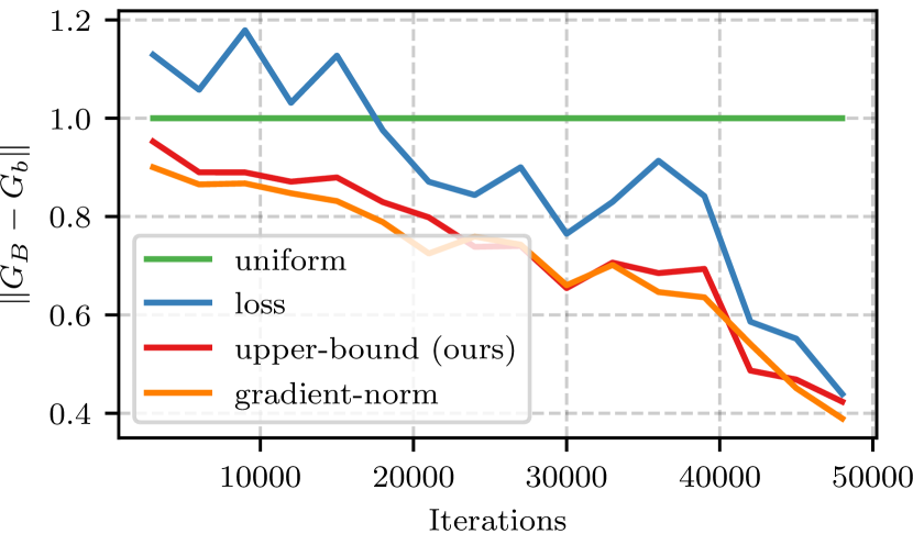
Figure 1: The y-axis denotes the $L_{2}$ distance of the average gradient of the large batch ($G_{B}$) and the average gradient of the small batch ($G_{b}$) normalized with the distance achieved by uniform sampling. The sampling of the small batch is done $10$ times and the reported results are the average. The details of the experimental setup are given in § 4.1.

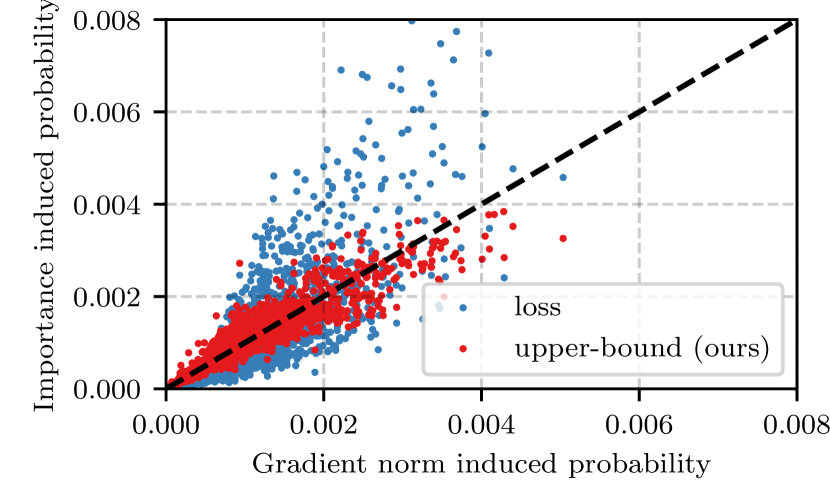
Figure 2: The probabilities generated with the loss and our upper-bound are plotted against the ideal probabilities produced by the gradient-norm. The black line denotes perfect correlation. The details of the experimental setup are given in § 4.1.

4.1 Ablation study

As already mentioned, several works Loshchilov & Hutter (2015); Schaul et al. (2015) use the loss value, directly or indirectly, to generate sampling distributions. In this section, we present experiments that validate the superiority of our method with respect to the loss in terms of variance reduction. For completeness, in the supplementary material we include a theoretical analysis that explains why sampling based on the loss also achieves variance reduction during the late stages of training.

Our experimental setup is as follows: we train a wide residual network Zagoruyko & Komodakis (2016) on the CIFAR100 dataset Krizhevsky (2009), following closely the training procedure of Zagoruyko & Komodakis (2016) (the details are presented in § 4.2). Subsequently, we sample $1,024$ images uniformly at random from the dataset. Using the weights of the trained network, at intervals of $3,000$ updates, we resample $128$ images from the large batch of $1,024$ images using uniform sampling or importance sampling with probabilities proportional to the loss, our upper-bound or the gradient-norm. The gradient-norm is computed by running the backpropagation algorithm with a batch size of 1.

Figure 1 depicts the variance reduction achieved with every sampling scheme in comparison to uniform. We measure this directly as the distance between the mini-batch gradient and the batch gradient of the $1,024$ samples. For robustness we perform the sampling $10$ times and report the average. We observe that our upper bound and the gradient norm result in very similar variance reduction, meaning that the bound is relatively tight and that the produced probability distributions are highly correlated. This can also be deduced by observing figure 2, where the probabilities proportional to the loss and the upper-bound are plotted against the optimal ones (proportional to the gradient-norm). We observe that our upper bound is almost perfectly correlated with the gradient norm, in stark contrast to the loss which is only correlated at the regime of very small gradients. Quantitatively the sum of squared error of $16,384$ points in figure 2 is $0.017$ for the loss and $0.002$ for our proposed upper bound.

Furthermore, we observe that sampling hard examples (with high loss), increases the variance, especially in the beginning of training. Similar behaviour has been observed in problems such as embedding learning where semi-hard sample mining is preferred over sampling using the loss Wu et al. (2017); Schroff et al. (2015).

4.2 Image classification

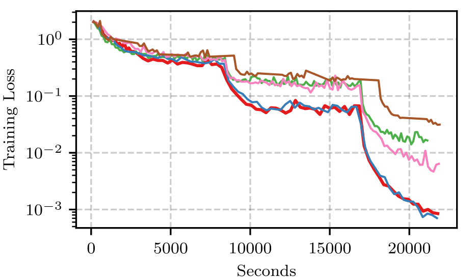
(a) CIFAR10 Training Loss

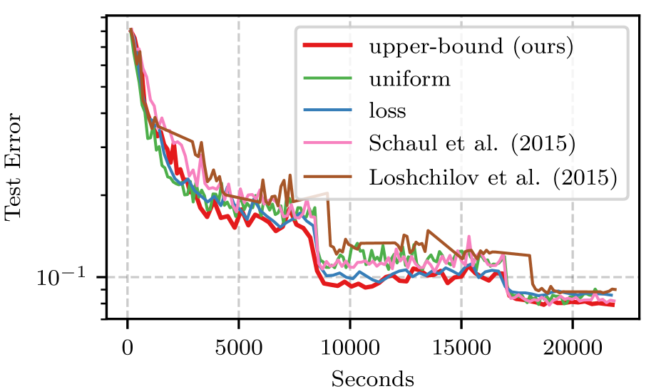
(b) CIFAR10 Test Error

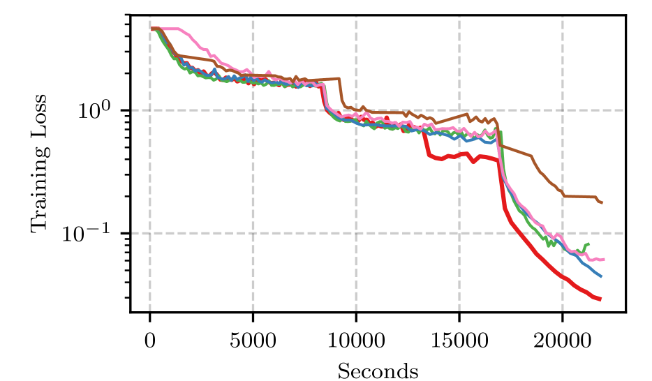
(c) CIFAR100 Training Loss

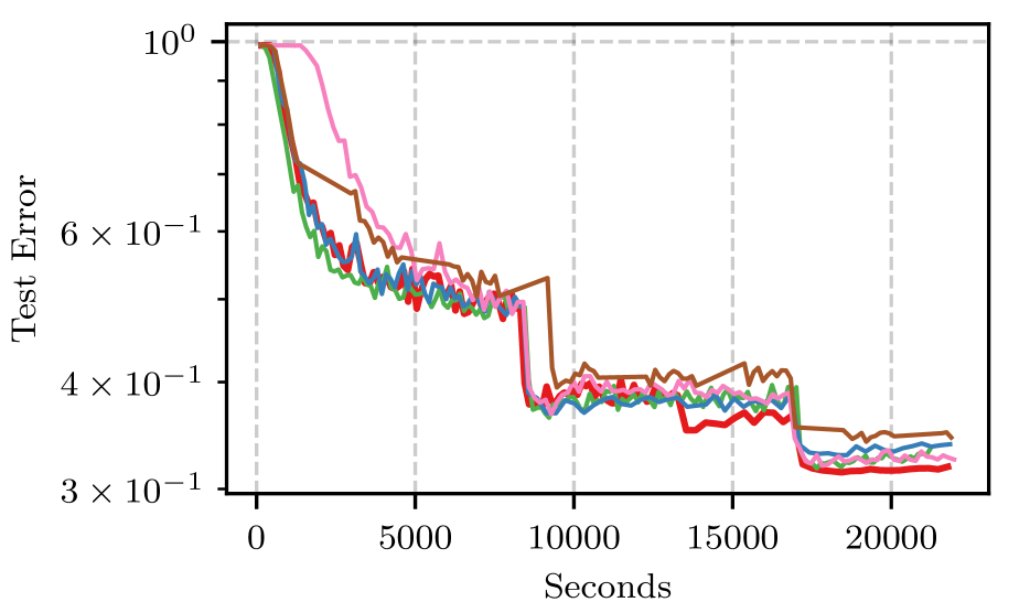
(d) CIFAR100 Test Error

Figure 3: Comparison of importance sampling using the upper-bound with uniform and loss based importance sampling. The details of the training procedure are given in § 4.2. Our proposed scheme is the only one achieving a speedup on CIFAR100 and results in 5% smaller test error. All presented results are averaged across $3$ independent runs.

In this section, we use importance sampling to train a residual network on CIFAR10 and CIFAR100. We follow the experimental setup of Zagoruyko & Komodakis (2016), specifically we train a wide resnet 28-2 with SGD with momentum. We use batch size $128$, weight decay $0.0005$, momentum $0.9$, initial learning rate $0.1$ divided by $5$ after $20,000$ and $40,000$ parameter updates. Finally, we train for a total of $50,000$ iterations. In order for our history based baselines to be compatible with the data augmentation of the CIFAR images, we pre-augment both datasets to generate $1.5\times 10^{6}$ images for each one. Our method does not have this limitation since it can work on infinite datasets in a true online fashion. To compare between methods, we use a learning rate schedule based on wall-clock time and we also fix the total seconds available for training. A faster method should have smaller training loss and test error given a specific time during training.

For this experiment, we compare the proposed method to uniform, loss, online batch selection by Loshchilov & Hutter (2015) and the history based sampling of Schaul et al. (2015). For the method of Schaul et al. (2015), we use their proportional sampling since the rank based is very similar to Loshchilov & Hutter (2015) and we select the best parameters from the grid $a=\{0.1,0.5,1.0\}$ and $\beta=\{0.5,1.0\}$. Similarly, for online batch selection, we use $s=\{1,10,10^{2}\}$ and a recomputation of all the losses every $r=\{600,1200,3600\}$ updates.

For our method, we use a presampling size of $640$. One of the goals of this experiment is to show that even a smaller reduction in variance can effectively stabilize training and provide wall-clock time speedup; thus we set $\tau_{th}=1.5$. We perform $3$ independent runs and report the average.

The results are depicted in figure 3. We observe that in the relatively easy CIFAR10 dataset, all methods can provide some speedup over uniform sampling. However, for the more complicated CIFAR100, only sampling with our proposed upper-bound to the gradient norm reduces the variance of the gradients and provides faster convergence. Examining the training evolution in detail, we observe that on CIFAR10 our method is the only one that achieves a significant improvement in the test error even in the first stages of training ($4,000$ to $8,000$ seconds). Quantitatively, on CIFAR10 we achieve more than an order of magnitude lower training loss and $8\%$ lower test error from $0.087$ to $0.079$ while on CIFAR100 approximately $3$ times lower training loss and $5\%$ lower test error from $0.34$ to $0.32$ compared to uniform sampling.

At this point, we would also like to discuss the performance of the loss compared to other methods that also select batches based on this metric. Our experiments show, that using “fresh” values for the loss combined with a warmup stage so that importance sampling is not started too early outperforms all the other baselines on the CIFAR10 dataset.

4.3 Fine-tuning

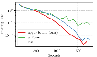
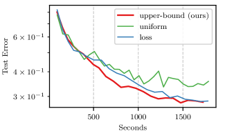
Figure 4: Comparison of importance sampling for fine-tuning on MIT67 dataset. The details of the training procedure are given in § 4.3. Our proposed algorithm converges very quickly to $28.06\%$ test error in approximately half an hour, a relative reduction of $17\%$ to uniform sampling. For robustness, the results are averaged across $3$ independent runs.

Our second experiment shows the application of importance sampling to the significant task of fine tuning a pre-trained large neural network on a new dataset. This task is of particular importance because there exists an abundance of powerful models pre-trained on large datasets such as ImageNet Deng et al. (2009).

Our experimental setup is the following, we fine-tune a ResNet-50 He et al. (2015) previously trained on ImageNet. We replace the last classification layer and then train the whole network end-to-end to classify indoor images among 67 possible categories Quattoni & Torralba (2009). We use SGD with learning rate $10^{-3}$ and momentum $0.9$. We set the batch size to $16$ and for our importance sampling algorithm we pre-sample $48$. The variance reduction threshold is set to $2$ as designated by equation 27.

To assess the performance of both our algorithm and our gradient norm approximation, we compare the convergence speed of our importance sampling algorithm using our upper-bound and using the loss. Once again, for robustness, we run $3$ independent runs and report the average.

The results of the experiment are depicted in figure 4. As expected, importance sampling is very useful for the task of fine-tuning since a lot of samples are handled correctly very early in the training process. Our upper-bound, once again, greatly outperforms sampling proportionally to the loss when the network is large and the problem is non trivial. Compared to uniform sampling, in just half an hour importance sampling has converged close to the best performance ($28.06\%$ test error) that can be expected on this dataset without any data augmentation or multiple crops Razavian et al. (2014), while uniform achieves only $33.74\%$.

4.4 Pixel by Pixel MNIST

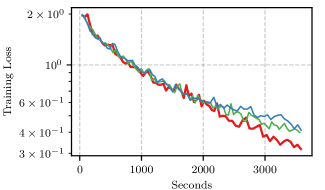
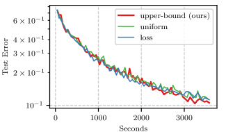
Figure 5: Comparison of importance sampling on pixel-by-pixel MNIST with an LSTM. The details of the training procedure are given in § 4.4. Our proposed algorithm speeds up training and achieves $7\%$ lower test error in one hour of training ($0.1055$ compared to $0.1139$). We observe that sampling proportionally to the loss actually hurts convergence in this case.

To showcase the generality of our method, we use our importance sampling algorithm to accelerate the training of an LSTM in a sequence classification problem. We use the pixel by pixel classification of randomly permuted MNIST digits LeCun et al. (2010), as defined by Le et al. (2015). The problem may seem trivial at first, however as shown by Le et al. (2015) it is particularly suited to benchmarking the training of recurrent neural networks, due to the long range dependency problems inherent in the dataset ($784$ time steps).

For our experiment, we fix a permutation matrix for all the pixels to generate a training set of $60,000$ samples with $784$ time steps each. Subsequently, we train an LSTM Hochreiter & Schmidhuber (1997) with $128$ dimensions in the hidden space, $\text{tanh}(\cdot)$ as an activation function and $\text{sigmoid}(\cdot)$ as the recurrent activation function. Finally, we use a linear classifier on top of the LSTM to choose a digit based on the hidden representation. To train the aforementioned architecture, we use the Adam optimizer Kingma & Ba (2014) with a learning rate of $10^{-3}$ and a batch size of $32$. We have also found gradient clipping to be necessary for the training not to diverge; thus we clip the norm of all gradients to $1$.

The results of the experiment are depicted in figure 5. Both for the loss and our proposed upper-bound, importance sampling starts at around $2,000$ seconds by setting $\tau_{th}=1.8$ and the presampling size to $128$. We could set $\tau_{th}=2.33$ (equation 27) which would only result in our algorithm being more conservative and starting importance sampling later. We clearly observe that sampling proportionally to the loss hurts the convergence in this case. On the other hand, our algorithm achieves $20\%$ lower training loss and $7\%$ lower test error in the given time budget.

5 Conclusions

We have presented an efficient algorithm for accelerating the training of deep neural networks using importance sampling. Our algorithm takes advantage of a novel upper bound to the gradient norm of any neural network that can be computed in a single forward pass. In addition, we show an equivalence of the variance reduction with importance sampling to increasing the batch size; thus we are able to quantify both the variance reduction and the speedup and intelligently decide when to stop sampling uniformly.

Our experiments show that our algorithm is effective in reducing the training time for several tasks both on image and sequence data. More importantly, we show that not all data points matter equally in the duration of training, which can be exploited to gain a speedup or better quality gradients or both.

Our analysis opens several avenues of future research. The two most important ones that were not investigated in this work are automatically tuning the learning rate based on the variance of the gradients and decreasing the batch size. The variance of the gradients can be kept stable by increasing the learning rate proportionally to the batch increment or by decreasing the number of samples for which we compute the backward pass. Thus, we can speed up convergence by increasing the step size or reducing the time per update.

6 Acknowledgement

This work is supported by the Swiss National Science Foundation under grant number FNS-30209 “ISUL”.

 

Appendix

 

Appendix A Differences of variances

In the following equations we quantify the variance reduction achieved with importance sampling using the gradient norm. Let $g_{i}\propto\left\lVert\nabla_{\theta_{t}}\mathcal{L}(\Psi(x_{i};\theta_{t}),y_{i})\right\rVert_{2}=\left\lVert G_{i}\right\rVert_{2}$ and $u=\frac{1}{B}$ the uniform probability.

We want to compute

$$\text{Tr}\left(\operatorname{\mathbb{V}}_{u}\!\left[G_{i}\right]\right)-\text{Tr}\left(\operatorname{\mathbb{V}}_{g}\!\left[w_{i}G_{i}\right]\right)\\ =\operatorname{\mathbb{E}}_{u}\!\left[\left\lVert G_{i}\right\rVert_{2}^{2}\right]-\operatorname{\mathbb{E}}_{g}\!\left[w_{i}^{2}\left\lVert G_{i}\right\rVert_{2}^{2}\right].$$ (28)

Using the fact that $w_{i}=\frac{1}{Bg_{i}}$ we have

$$\operatorname{\mathbb{E}}_{g}\!\left[w_{i}^{2}\left\lVert G_{i}\right\rVert_{2}^{2}\right]=\left(\frac{1}{B}\sum_{i=1}^{B}\left\lVert G_{i}\right\rVert_{2}\right)^{2},$$ (29)

thus

$$\text{Tr}\left(\operatorname{\mathbb{V}}_{u}\!\left[G_{i}\right]\right)-\text{Tr}\left(\operatorname{\mathbb{V}}_{g}\!\left[w_{i}G_{i}\right]\right)$$ (30)

$$=\frac{1}{B}\sum_{i=1}^{B}\left\lVert G_{i}\right\rVert_{2}^{2}-\left(\frac{1}{B}\sum_{i=1}^{B}\left\lVert G_{i}\right\rVert_{2}\right)^{2}$$ (31)

$$=\frac{\left(\sum_{i=1}^{B}\left\lVert G_{i}\right\rVert_{2}\right)^{2}}{B^{3}}\sum_{i=1}^{B}\left(B^{2}\frac{\left\lVert G_{i}\right\rVert_{2}^{2}}{(\sum_{i=1}^{B}\left\lVert G_{i}\right\rVert_{2})^{2}}-1\right)$$ (32)

$$=\frac{\left(\sum_{i=1}^{B}\left\lVert G_{i}\right\rVert_{2}\right)^{2}}{B}\sum_{i=1}^{B}\left(g_{i}^{2}-u^{2}\right).$$ (33)

Completing the squares at equation 33 and using the fact that $\sum_{i=1}^{B}u=1$ we complete the derivation.

$$\text{Tr}\left(\operatorname{\mathbb{V}}_{u}\!\left[G_{i}\right]\right)-\text{Tr}\left(\operatorname{\mathbb{V}}_{g}\!\left[w_{i}G_{i}\right]\right)$$ (34)

$$=\frac{\left(\sum_{i=1}^{B}\left\lVert G_{i}\right\rVert_{2}\right)^{2}}{B}\sum_{i=1}^{B}\left(g_{i}-u\right)^{2}$$ (35)

$$=\left(\frac{1}{B}\sum_{i=1}^{B}\left\lVert G_{i}\right\rVert_{2}\right)^{2}B\left\lVert g-u\right\rVert_{2}^{2}.$$ (36)

Appendix B An upper bound to the gradient norm

In this section, we reiterate the analysis from the main paper (§ 3.2) with more details.

Let $\theta^{(l)}\in\mathbb{R}^{M_{l}\times M_{l-1}}$ be the weight matrix for layer $l$ and $\sigma^{(l)}(\cdot)$ be a Lipschitz continuous activation function. Then, let

$$x^{(0)} =x$$ (37)

$$z^{(l)} =\theta^{(l)}\,x^{(l-1)}$$ (38)

$$x^{(l)} =\sigma^{(l)}(z^{(l)})$$ (39)

$$\Psi(x;\Theta) =x^{(L)}.$$ (40)

Equations 37-40 define a simple fully connected neural network without bias to simplify the closed form definition of the gradient with respect to the parameters $\Theta$.

In addition we define the gradient of the loss with respect to the output of the network as

$$\nabla_{x_{i}^{(L)}}\mathcal{L} =\nabla_{x_{i}^{(L)}}\mathcal{L}(\Psi(x_{i};\Theta),y_{i})$$ (41)

and the gradient of the loss with respect to the output of layer $l$ as

$$\nabla_{x_{i}^{(l)}}\mathcal{L}=\Delta_{i}^{(l)}\Sigma_{L}^{\prime}(z_{i}^{(L)})\nabla_{x_{i}^{(L)}}\mathcal{L}$$ (42)

where

$$\Delta_{i}^{(l)}=\Sigma_{l}^{\prime}(z_{i}^{(l)})\theta_{l+1}^{T}\dots\Sigma_{L-1}^{\prime}(z_{i}^{(L-1)})\theta_{L}^{T}$$ (43)

propagates the gradient from the last layer (pre-activation) to layer $l$ and

$$\Sigma_{l}^{\prime}(z)=diag\left(\sigma^{\prime(l)}(z_{1}),\dots,\sigma^{\prime(l)}(z_{M_{l}})\right)$$ (44)

defines the gradient of the activation function of layer $l$.

Finally, the gradient with respect to the parameters of the $l$-th layer can be written

$$\left\lVert\nabla_{\theta_{l}}\mathcal{L}(\Psi(x_{i};\Theta),y_{i})\right\rVert_{2}$$ (45)

$$= \left\lVert\left(\Delta_{i}^{(l)}\Sigma_{L}^{\prime}(z_{i}^{(L)})\nabla_{x_{i}^{(L)}}\mathcal{L}\right)\left(x_{i}^{(l-1)}\right)^{T}\right\rVert_{2}$$ (46)

$$\leq \left\lVert x_{i}^{(l-1)}\right\rVert_{2}\left\lVert\Delta_{i}^{(l)}\right\rVert_{2}\left\lVert\Sigma_{L}^{\prime}(z_{i}^{(L)})\nabla_{x_{i}^{(L)}}\mathcal{L}\right\rVert_{2}.$$ (47)

We observe that $x_{i}^{(l)}$ and $\Delta_{i}^{(l)}$ depend only on $z_{i}$ and $\Theta$. However, we theorize that due to various weight initialization and activation normalization techniques those quantities do not capture the important per sample variations of the gradient norm. Using the above, which is also shown experimentally to be true in § 4.1, we deduce the following upper bound per layer

$$\left\lVert\nabla_{\theta_{l}}\mathcal{L}(\Psi(x_{i};\Theta),y_{i})\right\rVert_{2}$$ (48)

$$\leq \max_{l,i}\left(\left\lVert x_{i}^{(l-1)}\right\rVert_{2}\left\lVert\Delta_{i}^{(l)}\right\rVert_{2}\right)\left\lVert\Sigma_{L}^{\prime}(z_{i}^{(L)})\nabla_{x_{i}^{(L)}}\mathcal{L}\right\rVert_{2}$$ (49)

$$= \rho\left\lVert\Sigma_{L}^{\prime}(z_{i}^{(L)})\nabla_{x_{i}^{(L)}}\mathcal{L}\right\rVert_{2},$$ (50)

which can then be used to derive our final upper bound

$$\left\lVert\nabla_{\Theta}\mathcal{L}(\Psi(x_{i};\Theta),y_{i})\right\rVert_{2}\leq\underbrace{L\rho\left\lVert\Sigma_{L}^{\prime}(z_{i}^{(L)})\nabla_{x_{i}^{(L)}}\mathcal{L}\right\rVert_{2}}_{\hat{G}_{i}}.$$ (51)

Intuitively, equation 51 means that the variations of the gradient norm are mostly captured by the final classification layer. Consequently, we can use the gradient of the loss with respect to the pre-activation outputs of our neural network as an upper bound to the per-sample gradient norm.

Appendix C Comparison with SVRG methods

For completeness, we also compare our proposed method with Stochastic Variance Reduced Gradient methods and present the results in this section. We follow the experimental setup of § 4.2 and evaluate on the augmented CIFAR10 and CIFAR100 datasets. The algorithms we considered were SVRG Johnson & Zhang (2013), accelerated SVRG with Katyusha momentum Allen-Zhu (2017) and, the most suitable for Deep Learning, SCSG Lei et al. (2017) which in practice is a mini-batch version of SVRG. SAGA Defazio et al. (2014) was not considered due to the prohibitive memory requirements for storing the per sample gradients.

For all methods, we tune the learning rate and the epochs per batch gradient computation ($m$ in SVRG literature). For SCSG, we also tune the large batch (denoted as $B_{j}$ in Lei et al. (2017)) and its growth rate. The results are depicted in figure 6. We observe that SGD with momentum performs significantly better than all SVRG methods. Full batch SVRG and Katyusha perform a small number of parameter updates thus failing to optimize the networks. In all cases, the best variance reduced method achieves more than an order of magnitude higher training loss than our proposed importance sampling scheme.

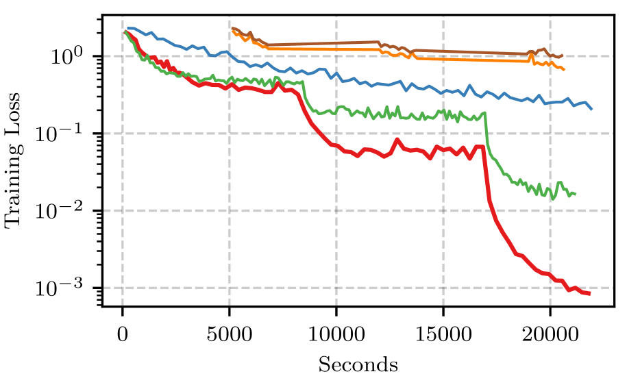
(a) CIFAR10 Training Loss

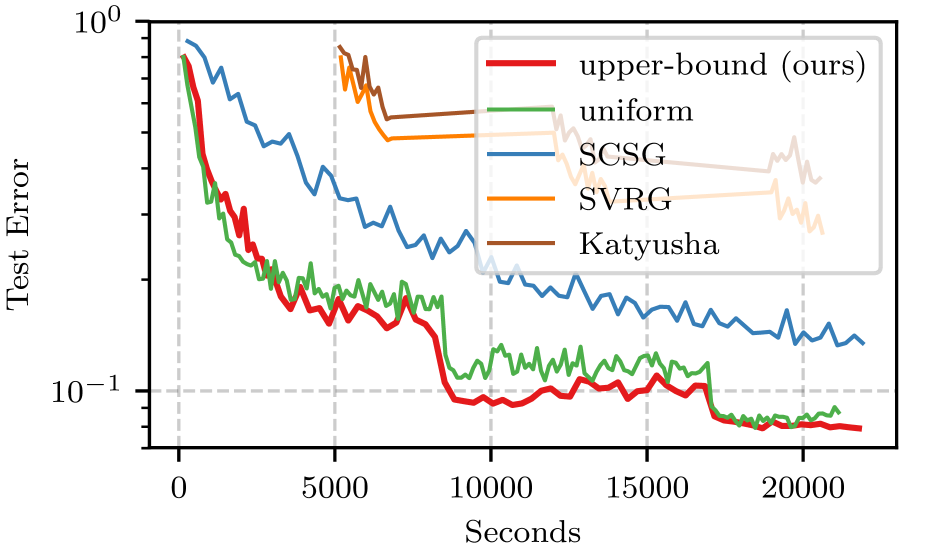
(b) CIFAR10 Test Error

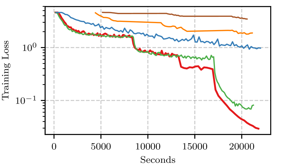
(c) CIFAR100 Training Loss

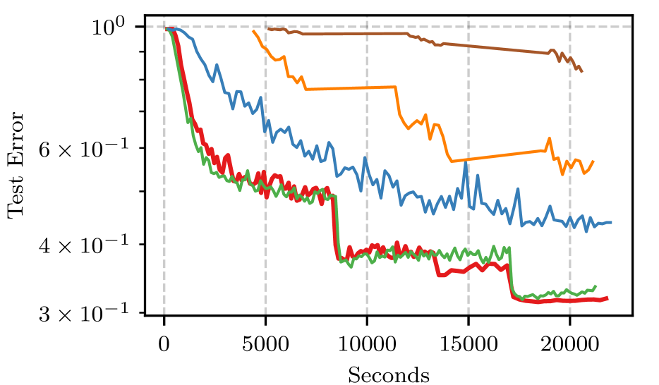
(d) CIFAR100 Test Error

Figure 6: Comparison of our proposed importance sampling scheme (upper-bound) to SGD with uniform sampling and variance reduced methods. Only SCSG can actually perform enough iterations to optimize the network. However, SGD with uniform sampling and our upper-bound greatly outperform SCSG.

Appendix D Ablation study on $B$

The only hyperparameter that is somewhat hard to define in our algorithm is the pre-sampling size $B$. As mentioned in the main paper, it controls the maximum possible variance reduction and also how much wall-clock time one iteration with importance sampling will require.

In figure 7 we depict the results of training with importance sampling and different pre-sampling sizes on CIFAR10. We follow the same experimental setup as in the paper.

We observe that larger presampling size results in lower training loss, which follows from our theory since the maximum variance reduction is smaller with small $B$. In this experiment we use the same $\tau_{th}$ for all the methods and we observe that $B=384$ reaches first to $0.6$ training loss. This is justified because computing the importance for $1,024$ samples in the beginning of training is wasteful according to our analysis.

According to this preliminary ablation study for $B$, we conclude that choosing $B=kb$ with $2<k<6$ is a good strategy for achieving a speedup. However, regardless of the choice of $B$, pairing it with a threshold $\tau_{th}$ designated by the analysis in the paper guarantees that the algorithm will be spending time on importance sampling only when the variance can be greatly reduced.

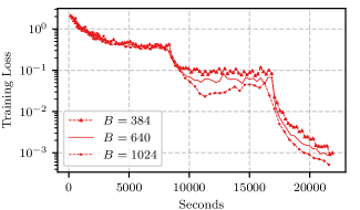
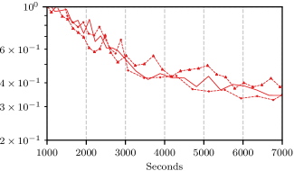
Figure 7: Results on training with different $B$ on CIFAR10. See the paper for the experimental setup.

Appendix E Importance Sampling with the Loss

In this section we will present a small analysis that provides intuition regarding using the loss as an approximation or an upper bound to the per sample gradient norm.

Let $\mathcal{L}(\psi,y):D\to\mathbb{R}$ be either the negative log likelihood through a sigmoid or the squared error loss function defined respectively as

$$\mathcal{L}_{1}(\psi,y) =-\log\left(\frac{\exp(y\psi)}{1+\exp(y\psi)}\right) y\in\{-1,1\}\quad\psi\in\mathbb{R}$$ (52)

$$\mathcal{L}_{2}(\psi,y) =\left\lVert y-\psi\right\rVert_{2}^{2} y\in\mathbb{R}^{d}\quad\psi\in\mathbb{R}^{d}$$

Given our upper bound to the gradient norm, we can write

$$\left\lVert\nabla_{\theta_{t}}\mathcal{L}(\Psi(x_{i};\theta_{t}),y_{i})\right\rVert_{2}\leq L\rho\left\lVert\nabla_{\psi}\mathcal{L}(\Psi(x_{i};\theta_{t}),y_{i})\right\rVert_{2}.$$ (53)

Moreover, for the losses that we are considering, when $\mathcal{L}(\psi,y)\to 0$ then $\left\lVert\nabla_{\psi}\mathcal{L}(\Psi(x_{i};\theta_{t}),y_{i})\right\rVert_{2}\to 0$. Using this fact in combination to equation 53, we claim that so does the per sample gradient norm thus small loss values imply small gradients. However, large loss values are not well correlated with the gradient norm which can also be observed in § 4.1 in the paper.

To summarize, we conjecture that due to the above facts, sampling proportionally to the loss reduces the variance only when the majority of the samples have losses close to 0. Our assumption is validated from our experiments, where the loss struggles to achieve a speedup in the early stages of training where most samples still have relatively large loss values.

References

- Abadi et al. (2016) Abadi, M., Agarwal, A., Barham, P., Brevdo, E., Chen, Z., Citro, C., Corrado, G. S., Davis, A., Dean, J., Devin, M., et al. Tensorflow: Large-scale machine learning on heterogeneous distributed systems. arXiv preprint arXiv:1603.04467, 2016.
- Alain et al. (2015) Alain, G., Lamb, A., Sankar, C., Courville, A., and Bengio, Y. Variance reduction in sgd by distributed importance sampling. arXiv preprint arXiv:1511.06481, 2015.
- Allen-Zhu (2017) Allen-Zhu, Z. Katyusha: The first direct acceleration of stochastic gradient methods. In Proceedings of the 49th Annual ACM SIGACT Symposium on Theory of Computing, pp. 1200–1205. ACM, 2017.
- Ba et al. (2016) Ba, J. L., Kiros, J. R., and Hinton, G. E. Layer normalization. CoRR, abs/1607.06450, 2016.
- Bengio et al. (2009) Bengio, Y., Louradour, J., Collobert, R., and Weston, J. Curriculum learning. In Proceedings of the 26th annual international conference on machine learning, pp. 41–48. ACM, 2009.
- Bordes et al. (2005) Bordes, A., Ertekin, S., Weston, J., and Bottou, L. Fast kernel classifiers with online and active learning. Journal of Machine Learning Research, 6(Sep):1579–1619, 2005.
- Canévet et al. (2016) Canévet, O., Jose, C., and Fleuret, F. Importance sampling tree for large-scale empirical expectation. In Proceedings of the International Conference on Machine Learning (ICML), pp. 1454–1462, 2016.
- Chollet et al. (2015) Chollet, F. et al. keras. https://github.com/fchollet/keras, 2015.
- Defazio et al. (2014) Defazio, A., Bach, F., and Lacoste-Julien, S. Saga: A fast incremental gradient method with support for non-strongly convex composite objectives. In Advances in neural information processing systems, pp. 1646–1654, 2014.
- Deng et al. (2009) Deng, J., Dong, W., Socher, R., Li, L.-J., Li, K., and Fei-Fei, L. ImageNet: A Large-Scale Hierarchical Image Database. In CVPR09, 2009.
- Fan et al. (2017) Fan, Y., Tian, F., Qin, T., Bian, J., and Liu, T.-Y. Learning what data to learn. arXiv preprint arXiv:1702.08635, 2017.
- Glorot & Bengio (2010) Glorot, X. and Bengio, Y. Understanding the difficulty of training deep feedforward neural networks. 2010.
- He et al. (2015) He, K., Zhang, X., Ren, S., and Sun, J. Deep residual learning for image recognition. arXiv preprint arXiv:1512.03385, 2015.
- Hochreiter & Schmidhuber (1997) Hochreiter, S. and Schmidhuber, J. Long short-term memory. Neural computation, 9(8):1735–1780, 1997.
- Ioffe & Szegedy (2015) Ioffe, S. and Szegedy, C. Batch normalization: Accelerating deep network training by reducing internal covariate shift. 2015.
- Johnson & Zhang (2013) Johnson, R. and Zhang, T. Accelerating stochastic gradient descent using predictive variance reduction. In Advances in neural information processing systems, pp. 315–323, 2013.
- Kingma & Ba (2014) Kingma, D. P. and Ba, J. Adam: A method for stochastic optimization. arXiv preprint arXiv:1412.6980, 2014.
- Krizhevsky (2009) Krizhevsky, A. Learning multiple layers of features from tiny images. Master’s thesis, Department of Computer Science, University of Toronto, 2009.
- Le et al. (2015) Le, Q. V., Jaitly, N., and Hinton, G. E. A simple way to initialize recurrent networks of rectified linear units. arXiv preprint arXiv:1504.00941, 2015.
- LeCun et al. (2010) LeCun, Y., Cortes, C., and Burges, C. Mnist handwritten digit database. AT&T Labs [Online]. Available: http://yann. lecun. com/exdb/mnist, 2, 2010.
- Lei et al. (2017) Lei, L., Ju, C., Chen, J., and Jordan, M. I. Non-convex finite-sum optimization via scsg methods. In Advances in Neural Information Processing Systems, pp. 2345–2355, 2017.
- Loshchilov & Hutter (2015) Loshchilov, I. and Hutter, F. Online batch selection for faster training of neural networks. arXiv preprint arXiv:1511.06343, 2015.
- Needell et al. (2014) Needell, D., Ward, R., and Srebro, N. Stochastic gradient descent, weighted sampling, and the randomized kaczmarz algorithm. In Advances in Neural Information Processing Systems, pp. 1017–1025, 2014.
- Quattoni & Torralba (2009) Quattoni, A. and Torralba, A. Recognizing indoor scenes. In Computer Vision and Pattern Recognition, 2009. CVPR 2009. IEEE Conference on, pp. 413–420. IEEE, 2009.
- Razavian et al. (2014) Razavian, A. S., Azizpour, H., Sullivan, J., and Carlsson, S. Cnn features off-the-shelf: an astounding baseline for recognition. In Computer Vision and Pattern Recognition Workshops (CVPRW), 2014 IEEE Conference on, pp. 512–519. IEEE, 2014.
- Richtárik & Takáč (2013) Richtárik, P. and Takáč, M. On optimal probabilities in stochastic coordinate descent methods. arXiv preprint arXiv:1310.3438, 2013.
- Schaul et al. (2015) Schaul, T., Quan, J., Antonoglou, I., and Silver, D. Prioritized experience replay. arXiv preprint arXiv:1511.05952, 2015.
- Schroff et al. (2015) Schroff, F., Kalenichenko, D., and Philbin, J. Facenet: A unified embedding for face recognition and clustering. In Proceedings of the IEEE conference on computer vision and pattern recognition, pp. 815–823, 2015.
- Simo-Serra et al. (2015) Simo-Serra, E., Trulls, E., Ferraz, L., Kokkinos, I., Fua, P., and Moreno-Noguer, F. Discriminative learning of deep convolutional feature point descriptors. In Computer Vision (ICCV), 2015 IEEE International Conference on, pp. 118–126. IEEE, 2015.
- Wang et al. (2016) Wang, L., Yang, Y., Min, M. R., and Chakradhar, S. Accelerating deep neural network training with inconsistent stochastic gradient descent. arXiv preprint arXiv:1603.05544, 2016.
- Wu et al. (2017) Wu, C.-Y., Manmatha, R., Smola, A. J., and Krahenbuhl, P. Sampling matters in deep embedding learning. In The IEEE International Conference on Computer Vision (ICCV), Oct 2017.
- Zagoruyko & Komodakis (2016) Zagoruyko, S. and Komodakis, N. Wide residual networks. In Richard C. Wilson, E. R. H. and Smith, W. A. P. (eds.), Proceedings of the British Machine Vision Conference (BMVC), pp. 87.1–87.12. BMVA Press, September 2016. ISBN 1-901725-59-6. doi: 10.5244/C.30.87. URL https://dx.doi.org/10.5244/C.30.87.
- Zhao & Zhang (2015) Zhao, P. and Zhang, T. Stochastic optimization with importance sampling for regularized loss minimization. In Proceedings of the 32nd International Conference on Machine Learning (ICML-15), pp. 1–9, 2015.