Galerkin-Collocation domain decomposition method for arbitrary binary black holes
Abstract
We present a new computational framework for the Galerkin-collocation method for double domain in the context of ADM 3+1 approach in numerical relativity. This work enables us to perform high resolution calculations for initial sets of two arbitrary black holes. We use the Bowen-York method for binary systems and the puncture method to solve the Hamiltonian constraint. The nonlinear numerical code solves the set of equations for the spectral modes using the standard Newton-Raphson method, LU decomposition and Gaussian quadratures. We show convergence of our code for the conformal factor and the ADM mass. Thus, we display features of the conformal factor for different masses, spins and linear momenta.
I Introduction
The recent direct observation of gravitational waves by the LIGO-Virgo consortium ligo1 ; ligo2 ; ligo3 ; ligo4 represents an enormous breakthrough the researchers have pursued for decades. The observed wave template was generated by a binary black hole (BBH) system as predicted by the numerical simulations. In fact, Numerical General Relativity was crucial after a long effort of theoretical developments towards the obtention of a stable full dynamics of a BBH pretorius ; campanelli ; baker . In this context, it is necessary a precise determination of the initial spatial hypersurface which contains the desired astrophysical configuration.
We report here a new domain decomposition algorithm (DD) based on the Galerkin-Collocation (GC) method GC_method to obtain general initial data for a BBH system. In the present version, we are going to restrict ourselves to the Bowen-York initial data bowen-york with the puncture brandt wormhole foliations representing the black holes, but it can be extended to the case of puncture trumpet representation baum_naculich ; hannam_09 . Albeit the existence of other spectral DD codes due to Grandclement et al. grandclement , Pfeiffer pfeiffer ; pfeiffer_CPC , Ansorg ansorg_05 ; ansorg_07 and Ossokine et al.ossokine , we believe that the present approach is a viable and valid alternative to the established codes. In the sequence, we present unique aspects of the GC-DD method that makes it structurally simple and at the same time accurate.
The present GC-DD algorithm is a direct extension of the single domain scheme clemente we have developed recently to describe the initial data for single and binary black holes punctures in the wormhole or trumpet representations. We highlight some of the distinct aspects of the GC domain decomposition algorithm. The basis functions are established such that each component satisfies the boundary conditions in each subdomain. We have introduced two subdomains covered by the standard spherical coordinates designated by and . In this scheme, the angular coordinates of the collocation points are common to both subdomains, although we can to chose different numbers of collocation points in each domain. We have selected the spherical harmonics as the angular basis functions. Another distinct feature of the algorithm is the particular way we have compactified the spatial domain (cf. Fig. 1).
We have organized the paper as follows. In Section II, we have briefly described the main aspects of the initial data construction of spinning-boosted binaries of black holes. Section III deals with the essential features of the GC-DD method to solve the Hamiltonian constraint. The numerical implementation of the code is described in Section IV. We have presented in Section V the validation of the algorithm with three examples of binary systems. The first and the second are equal masses boosted binary black holes in the axisymmetric and three-dimensional configurations, respectively. Whereas in the last example we have treated a more general binary of spinning-boosted black holes of different puncture masses. In all cases, we have exhibited the convergence tests. We summarize to conclude, and we discuss of possible applications of the algorithm considered here.
II Basic equations
In General Relativity the initial data problem deals with the characterization of the gravitational and matter fields in a given initial spatial hypersurface. Equivalently, this task entails the establishment of an initial hypersurface containing plausible astrophysical systems such as binary black holes, binary of neutron stars or a binary formed by a neutron star and a black hole. According to the 3+1 formulation of the General Relativity adm ; gourgoulhon , the spacetime is foliated by a family of spatial slices . Assuming the absence of matter fields, we have to solve the Hamiltonian and momentum constraint equations for - the 3-metric and the extrinsic curvature associated with the initial slice, respectively - after providing their corresponding freely specifiable components.
The Hamiltonian and momentum constraints have the following forms that encompass the above requirements cook
| (1) | |||
| (2) |
where is the known spatial background metric that is related to through the conformal transformation
| (3) |
Then, all barred quantities are related to the background metric and
| (4) |
is the traceless part of the extrinsic curvature related to its counterpart of the background metric.
The simplest choice for the background spatial metric is and together with the maximal slicing condition, , provide the decoupling of Eqs. (1) and (2). As a consequence, the momentum constraint becomes a linear equation allowing to obtain the exact solutions for the components of corresponding to spinning and boosted black holes. This scheme characterizes the well known Bowen-York initial data bowen-york .
To describe binary black holes, we have considered the puncture method brandt in which the singularities present in the conformal factor are described analytically by representing each black hole in the wormhole or trumpet slices. In the first case, the ansatz for the conformal factor is
| (5) |
where and are the puncture masses, denotes the coordinate distance to the center of the black hole located at and is a regular function determined after solving the Hamiltonian constraint.
In the single domain Galerkin-Collocation algorithm clemente , we have adopted spherical coordinates to cover the whole spatial domain. In the present two domain approach, we have used the same spherical coordinates in both domains instead of alternative coordinate systems as in Refs. pfeiffer ; pfeiffer_CPC ; ansorg_05 ; ansorg_07 . In this case, the regular function satisfies the Robin boundary condition
| (6) |
for a large distance from the binary.
After substituting the conformal factor given by Eq. (5) into the Hamiltonian constraint, we obtain
| (7) | |||||
The first three terms correspond to the Laplacian of the function in spherical coordinates, and depends upon the black holes have linear and angular momenta. Due to the linearity of the momentum constraint equation, the total background extrinsic curvature corresponding to an arbitrary binary black hole is
| (8) |
where and correspond, respectively, to the background extrinsic curvature of the puncture located at , , carrying linear momentum and spin . For the sake of completeness, we have bowen-york ; baumgarte
| (9) | |||||
| (10) |
where indicate each black hole and is the normal vector to .
To complete this section we introduce the ADM mass for the arbitrary binary black holes baumgarte
| (11) |
where is a surface at infinity on the spacelike foliation ; is an outward surface element. By assuming spherical coordinates and the conformal factor given by Eq. (5), we obtain
| (12) |
where .
III The Galerkin-Collocation decomposition method
We present here the GC domain decomposition algorithm to obtain initial data representing binary black holes. As the first step, we have divided the spatial domain into two subdomains denoted by and , where indicates the interface of these two non-overlapping subdomains. As a consequence, both subdomains share the same spherical angular coordinates which simplifies the implementation of the algorithm considerably.
The centerpiece of the algorithm is the spectral approximations of the regular functions given by
| (13) |
where denotes the subdomains , represents the unknown coefficients or modes, and are, respectively, the radial and angular truncation orders that limit the number of terms in the above expansion. The angular patch has the spherical harmonics, , as the basis functions that are common to both domains. The choice of spherical coordinates together with the adoption of spherical harmonics basis functions are quite natural, and as we are going to show, are computationally very efficient and accurate. The radial basis functions are defined following the prescription of the Galerkin method canuto ; boyd , in the sense of each function must satisfy the boundary conditions. Usually, they are obtained by taking suitable linear combinations of the Chebyshev polynomials as we are going to describe.
Before defining the radial basis functions, it is necessary to introduce the computational subdomains. We have considered this feature an innovative part in constructing the algorithm. The Fig. 1 illustrates the mapping we have adopted. First, the entire radial domain is mapped onto the interval through the algebraic map boyd
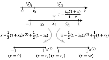
| (14) |
where is the map parameter. The subdomains and are now characterized by and , respectively; is related to the interface radial coordinate by . And second, we further define linear transformations , for the new computational domains for and , respectively, such that (cf. Fig. 1). The collocation points are designated by and mapped back to in the radial physical domain.
We are now in conditions to define the radial basis functions in each subdomain. With respect to , we define by
| (15) |
where is the Chebyshev polynomial of th order, and corresponds to . For the second domain , we have
| (16) |
where is the redefined Chebyshev polynomial of th order according to
| (17) |
In this case the interval is mapped out to . With the definition (15) it can be shown that each basis function behaves asymptotically as . Therefore, we obtain the following asymptotic expression in the second domain
| (18) |
where the function embodies the contribution to the ADM mass due to presence of angular and linear momenta. We can determine from
| (19) |
and the calculation of the ADM mass using Eq. (12) becomes straightforward.
The spherical harmonics are complex functions implying that the coefficients must be complex. Since the conformal factor is a real function, the real and imaginary parts of satisfy the following symmetry relations
| (20) |
due to . Consequently, the number of independent coefficients in each domain is .
We have to guarantee that the spectral approximations of and given by expression (13) represent the same function at the match point of the domain. This is done by imposing the continuity at the interface that separates both subdomains through the following matching conditions
We now establish the residual equation associated with the Hamiltonian constraint in each domain by substituting the spectral approximations represented by Eq. (13) into the Hamiltonian constraint (7). In addition, we have taken into account the differential equation for the spherical harmonics to get rid of the derivatives with respect to and . We have arrived to the following expression
| (22) |
with corresponding to the domains and , respectively.
The next and final step is to describe the procedure to obtain de coefficients . We have followed the implementation of one domain clemente straightforwardly. From the method of weighted residuals finlayson , these coefficients are evaluated with the condition of forcing the residual equation to be zero in an average sense. It means that
| (23) |
where the functions and are called the test functions while and are the corresponding weights. In both domains we choose the radial test function as prescribed by the Collocation method boyd ; fornberg :
| (24) |
which is the delta of Dirac function, , , represents the collocation points defined in each domain and . Following the Galerkin method we identify the angular test function as the spherical harmonics and as a consequence . Therefore Eq. (23) becomes
| (25) |
where , and . As we are going to show, the number of radial collocation points defined in each domain provides the correct number of equations for the modes.
Before going further, we need to consider the matching conditions in respect to the approximation adopted above. The corresponding residuals and are approximated as
| (26) |
where and . Notice that these expressions result from exact integrations on the angular domain (cf. Eq. (23)) due to the orthogonality of the spherical harmonics. Thus, we ended up with linear relations of the coefficients of both domains.
At this point we present the radial collocation points at each domain. By taking into account the matching conditions, we have unknown coefficients in both domains, therefore it is necessary the same number of equations resulting from Eq. (25). Thus, we need radial collocation points in each computational subdomain given by
| (27) |
and the corresponding radial points in the corresponding physical subdomain are
| (28) | |||||
| (29) |
with . We remark that the point at infinity is excluded since the residual equation is automaticaly satisfied asymptotically due to the choice of the radial basis function (16). Noticed that the origin is also excluded. For the sake of illustration, we show in Fig. 2 the organization of the radial collocation points in both subdomains.
We are in conditions to present a more detailed form of the set of equations represented by Eq. (22), after using the orthogonality of the spherical harmonics in the first two terms of the residual equation (25):
| (30) |
where , and . Therefore, we have obtained a total nonlinear algebraic equations, that together with the equations from the matching conditions (26), constitute the set of equations to be solved for the modes . As a final piece of information, we have calculated the last term of the above equation using quadrature formulae as indicated below
| (31) |
where , , are the quadrature collocation points, and are the corresponding weights fornberg . For better accuracy we have set , but this is not mandatory since it is possible to use simply .
In closing this Section, it is useful to comment on the possibility of damaging the exponential convergence of the numerical solution to the Hamiltonian constraint due to the singularities of the punctures. The first is to choose another form of the conformal factor with the requirement of being regular everywhere as established by the moving puncture method and applied to the initial data problem in connection with trumped black holes baumgarte_12 ; dietrich . Alternatively, it is possible to set suitable coordinates in which the puncture are located at the edge of the computational domain, or as adopted in Refs. ansorg_05 ; ansorg_07 in placing the punctures at the domain interface. We have followed the latter approach (cf. Fig. 2) avoiding to coincide any collocation point coinciding with the loci of the punctures. As we are going to show in the next Section, the exponential convergence in all examples.
IV Numerical implementation
The computational framework was implemented initially in Maple. The Maple quasi-numerical script was used as a reference to develop a serial code in Fortran. Although algorithmically different, both programs produced the same output for monitored variables. This constituted an excellent validation of the Fortran code. In this work, we had used only the numerical code in Fortran when the memory and the velocity were a real limit for simulations. In turn, the Fortran solver allowed us to identify the stage that needed more computational resources. Thus, we have implemented a parallelization to proceed with the determination of the desired solution.
Our numerical problem has nonlinear equations from the Hamiltonian constraint (30) and linear equations from the matching conditions (26). These three sets of equations are deployed in one vector , with , and . The system of equations has solutions; each solution corresponds to one and only one real (or imaginary) part of the coefficient .
To solve the system of equations, we use the standard Newton-Raphson method NumericalRecipes
| (32) |
where is the Jacobian matrix and is the variation of the solution between the iteration and , up to some specified tolerance for the convergence. We stress here the fact that the Jacobian is calculated numerically using forward finite differences with excellent results. To get the set of solutions at each iteration, we use an LU or QR decomposition NumericalRecipes . We observe the best performance for the LU decomposition. All the special functions and its derivatives are calculated using the standard generating formulae from the Numerical Recipes library of subroutines.
V Numerical Results
We have considered three examples of initial data of binary black holes to show the fast convergence of the domain decomposition Galerkin-Collocation algorithm. We have started with an axisymmetric configuration of boosted black holes and in the sequence, two distinct three-dimensional binary systems formed with black holes with angular and linear momenta.
The first example consists of two boosted black holes represented by punctures of equal masses and . The punctures are placed on the axis at and , respectively, where is the coordinate separation between the punctures. The corresponding linear momenta are and which yields the following expression for source-term of the Hamiltonian:
| (33) |
where . Notice that since does not depend on the angle ; we have an axisymmetric configuration. In this case, the Legendre polynomials replace the spherical harmonics as the angular basis functions in the spectral approximation of Eq. (13). Alternatively, we can translate the axisymmetry in the spectral representation by for all .
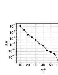
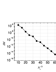
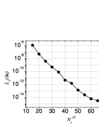
For the numerical convergence tests, we have chosen , and fix , . Then, we have proceeded by varying the radial truncation order of the second domain as and solved the system of Eqs. (26) and (30) for each . With the modes determined, the ADM mass is calculated according to Eqs. (12) and (19). In the sequence, we have evaluated the difference between the ADM masses corresponding to successive solutions through . Fig. 3 shows the exponential decay of indicating the rapid convergence of the numerical solution. Note that for the saturation due to round-off error is achieved in about . In these numerical experiments, we have chosen for the interface and the map parameter. The ADM mass of the axisymmetric binary of boosted black hole is .
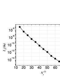
Another convergence test is provided by the decay of the -error between two successive solutions of the regular function obtained previously. We have calculated the -error using the following expression
| (34) |
where and . From Fig. 3, the exponential convergence is achieved similarly to the convergence of the ADM M mass.
The second example is the three-dimensional boosted binary of black holes studied by Ansorg et al. ansorg_04 . The punctures have the same masses with , and lie on the axis at and . The linear momenta of the punctures are and and the corresponding source-term becomes
| (35) | |||||
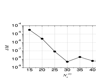
where . With , we ended up with a particular expression that induces additional symmetries for the coefficients , meaning that some of the coefficients vanishes. In this case, we have found that all imaginary parts of the coefficients vanish, , and some of the real coefficients according to if is an odd number. We have performed the convergence tests of the ADM mass and the error associated with the difference between two successive solutions in the second domain. The results depicted in Fig. 4 present similar exponential decay suggesting we can select one of the tests to verify the convergence of the code. In the numerical experiments, we have set as before , and the ADM mass of the three-dimensional boosted binary system is . Ansorg et al. ansorg_04 have used a grid of points, whereas we have used a total of 920 coefficients in the highest resolution of . Note that with these values the total number of coefficients would be , but the additional symmetries have reduced it drastically, moreover we have required a total of grid points (here for the quadrature formulae (31)).
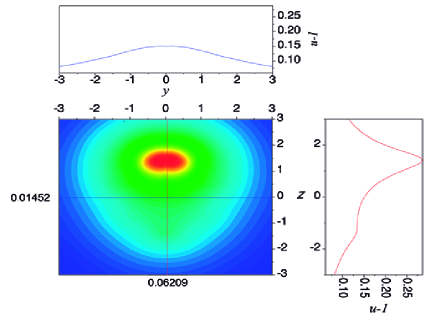
The last example is a general three-dimensional initial data of a binary of spinning-boosted black holes. This initial configuration is taken from Brügmann brugman_99 in which the puncture masses are , located at and , respectively. The linear and angular momenta of each puncture are , , and , where and .
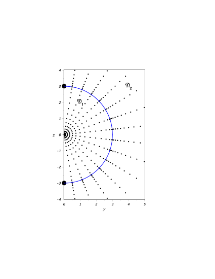
We have omitted writing here the long expression of the source-term , but contrary to the previous examples there are no additional symmetries reduce the number of independent coefficients other than expressed by Eq. (20). Further, we have restricted to verify the convergence of the ADM mass evaluating the quantity as already established, remarking that we have set and . Fig. 5 shows a clear exponential decay of until . To complete all the pertinent information for the numerical experiments, we have set as in the other two examples, and the calculated ADM mass is . It seems that these choices for the location of the interface as well the map parameter in the present code is general for any binary black hole system. This system was solved using the BAM code bam_brug with a grid of points, while in the present algorithm we have required the maximum of coefficients in both domains for . For the sake of illustration, after expressing the regular function in terms of the cartesian coordinates, i.e. , we have projected into the plane as shown in Fig. 6. Notice the asymmetry due to the distinct spins of both black holes.

VI Concluding remarks and outlook of future work
We have presented a new DD code base on the GC method for the Bowen-York initial data representing arbitrary binary black hole systems. It is worth of mentioning some of the leading aspects of the algorithm that makes it simpler and distinct from other numerical procedures.
In the present algorithm, we have covered the whole spatial domain with the spherical coordinates no matter which binary system is under consideration. We have split the spatial domain into two subdomains defined by and , such that the angular coordinates of the collocation points are the same for both subdomains as indicated by Fig. 2. As the central piece of the code, we have provided the spectral approximation of the regular component of the conformal factor in each subdomain, , with the spherical harmonics as the angular basis functions. The radial basis functions are defined in each subdomain to satisfy the boundary conditions.
We have solved the Hamiltonian constraint (7) for three distinct BBH represented by punctures located on the axes. The first is an axisymmetric boosted binary; the second example is a three-dimensional binary boosted taken from Ansorg et al. ansorg_04 . In both cases the puncture masses are equal. The third example is an arbitrary spinning-boosted binary of distinct puncture masses drawn from Ref. brugman_99 . The tests we have employed to validate the code was the convergence of the ADM mass and the regular function . As expected the convergence is exponential as shown by the Figures.
The details of the code performance and its parallelization for massive computations will be addressed elsewhere. Meanwhile, we only mention here that the first two binary systems were solved using one thread for computations. In the last example, however, we required multi-threading to deal with the Hamiltonian constraint.
The present algorithm can be applied to some problems. The most relevant is the obtention of high-resolution initial data for a binary system of neutron stars. For the BBH system, we can straightforwardly consider trumpets instead wormholes representations. Moreover, we could use the conformal thin sandwich approach for the initial data. These are just some possible directions and venues for our coming work, including evolutions.
Acknowledgements.
The authors acknowledge the financial support of the Brazilian agencies Conselho Nacional de Desenvolvimento Científico e Tecnológico (CNPq) and Fundação Carlos Chagas Filho de Amparo à Pesquisa do Estado do Rio de Janeiro (FAPERJ). H. P. O. thanks FAPERJ for support within the Grant No. E-26/202.998/518 2016 Bolsas de Bancada de Projetos (BBP).References
- (1) B. P. Abbott et al., Phys. Rev. Lett. 116, 061102 (2016).
- (2) B. P. Abbott et al., Phys. Rev. Lett. 116, 241103 (2016).
- (3) B. P. Abbott et al., Phys. Rev. Lett. 118, 221101 (2017).
- (4) B. P. Abbott et al., Phys. Rev. Lett. 119, 141101 (2017).
- (5) F. Pretorius, Phys. Rev. Lett. 95, 121101 (2005).
- (6) M. Campanelli, C. O. Lousto, P. Marroneti and Y. Zlochower, Phys. Rev. Lett. 96, 111102 (2006).
- (7) J. G. Baker, J. Centrella, D. -I. Choi, M. Koppitz and J. van Meter, Phys. Rev. Lett. 96, 111102 (2006).
- (8) H. P. de Oliveira and E. L. Rodrigues, Class. Quant. Grav. 28, 235011 (2011); H. P. de Oliveira, E. L. Rodrigues and J. F. E. Skea, Phys. Rev. D 84, 044007 (2011).
- (9) J. M. Bowen and J. W. York, Phys. Rev. D 21, 2047 (1980).
- (10) S. Brandt and B. Brugmann, Phys. Rev. Lett. 78, 3606 (1997).
- (11) T. W. Baumgarte and S. G. Naculich, Phys. Rev. D 75, 067502 (2007).
- (12) M. Hannam, S. Husa and N. Ó Murchada, Phys. Rev. D 80, 124007 (2009).
- (13) P. Grandclement, S. Bonazzola, E. Gourgoulhon and J.-A. Mark, J. Comp. Phys. 170, 231 (2000).
- (14) H. P. Pfeiffer, Initial data for black hole evolutions, PhD thesis, preprint arXiv: gr-qc/0510016.
- (15) H. P. Pfeiffer, Lawrence E. Kidder, Mark A. Scheel and Saul Teukolsky, Comp. Phys. Commun. 152, 253 (2003).
- (16) M. Ansorg, Phys. Rev. D 72, 024018 (2005).
- (17) M. Ansorg, Class. Quant. Grav. 24, S1-14 (2007).
- (18) S. Ossokine, F. Foucart, H. Pfeiffer, M. Boyle and B. Szilágyi, Class. Quant. Grav. 32, 245010 (2015).
- (19) P. M. C. Clemente and H. P. de Oliveira, Phys. Rev. D 96, 024035 (2017).
- (20) R. Arnowitt, S. Deser and C. W. Misner, The dynamics of general relativity, in Gravitation: An Introduction to Current Research, ed. L. Witten (Wiley, New York, 1962), p.227.
- (21) E. Gourgoulhon, J. Phys. Conf. Ser. 91, 012001 (2007).
- (22) G. B. Cook, Initial Data for Numerical Relativity, Liv. Rev. Relativity, 3, 5 (2000).
- (23) T. Baumgarte and S. L. Shapiro, Numerical Relativity - Solving the Einstein’s Equations on the Computer, Cambridge University Press (2010).
- (24) C. Canuto, M. Y. Hussaini, A. Quarteroni and T. A. Zang, Spectral Methods in Fluid Dynamics (Springer-Verlag, Berlin, Germany; Heidelberg, Germant, 1988); Spectral Methods: Fundamentals in Single Domains (Springer-Verlag, Berlin, Germany; Heidelberg, Germant, 2006); Roger Peyert, Spectral Methods for Incompressible Viscous Flow, Springer(2001).
- (25) J. P. Boyd, Chebyshev and Fourier Spectral Methods (Dover Publications, New York, 2001).
- (26) B. A. Finlayson, The Method of Weighted Residuals and Variational Principles (Academic Press, New York, 1972).
- (27) B. Fornberg, A Pratical Guide to Pseudospectral Methods, Cambridge Monographs on Applied and Computational Mathematics, Cambrige University Press (1998).
- (28) T. W. Baumgarte, Phys. Rev. D 85, 084013 (2012).
- (29) T. Dietrich and B. Brugmann, Phys. Rev. D 89, 024014 (2014).
- (30) W. H. Press, S. A. Teukolsky, W. T. Vetterling and B. P. Flannery, Numerical Recipes 3rd Edition: The Art of Scientific Computing, Cambridge University Press (2007).
- (31) M. Ansorg, B. Brugmann and W. Tichy, Phys. Rev. D 70, 064011 (2004).
- (32) B. Brugmann, Int. J. Mod. Phys. D 8, 85 (1999).
- (33) B. Brügmann, Bifunctional adaptive mesh (BAM) for 3d numerical relativity, in Eighteenth Texas Symposium on Relativistic Astrophysics and Cosmology (Chicago, 1996), eds. A. Olinto, J. Frieman and D. Schramm (World Scientific Publishing, Singapore, 1998).