Interference in spin-orbit coupled transverse magnetic focusing; emergent phase due to in-plane magnetic fields

Abstract

Spin-orbit (SO) interactions in two dimensional systems split the Fermi surface, and allow for the spatial separation of spin-states via transverse magnetic focusing (TMF). In this work, we consider the case of combined Rashba and Zeeman interactions, which leads to a Fermi surface without cylindrical symmetry. While the classical trajectories are effectively unchanged, we predict an additional contribution to the phase, linear in the applied in-plane magnetic field. We show that this term is unique to TMF, and vanishes for magnetic (Shubnikov de Haas) oscillations. Finally we propose some experimental signatures of this phase.

I Introduction

Transverse magnetic focusing (TMF) has a long history, being employed in metals and semi-conductors, and has been used to investigate the shape of the Fermi surfaceSharvin1965 ; Sharvin1965a ; Tsoi1974 ; Tsoi1999 ; Vanhouten . A TMF experiment consists of a source and a detector, separated by a distance $l$, with charges focused from the source to the detector via a weak transverse magnetic field. It is the direct translation of charge mass spectroscopy to the solid state. Despite the nearly half century of experimental history, TMF is still producing novel results, with the most recent application in systems with non-quadratic dispersion relations, such as GrapheneTaychatanapat2013 and two dimensional charge gases with large spin-orbit (SO) interactionsRokhinson2004 . In spin-orbit coupled systems, the spin-split Fermi surfaces result in a “doubled” focusing peak, which provides a novel platform investigations of polarisation effects in the source and detector quantum point contactsUsaj2004 ; Rokhinson2006 . The separation of the peaks also allows for the direct determination of the magnitude of the spin-orbit splitting, hence TMF can be used in addition to quantum magnetic oscillations to yield detailed information about spin-orbit coupled electron and hole systems.

Much of the theoretical and experimental work concerning TMF with large spin-orbit splittings has considered a singular dominant SO interaction. This leads to a cylindrically symmetric Fermi surface, and a double peak structure that is, in essence, two copies of the single peak structureZulicke2007 . This assumption is well justified for many typical experimental systems grown along high symmetry crystal axes, as classical trajectories are not significantly altered except in the case of extremely large asymmetryBladwell2015 . While a sufficiently large secondary SO interaction can lead to magnetic breakdown like behaviourReynoso2007 , the requirement for resolution of the double peak structure means that the typical regime is one characterised by the secondary SO interaction being weaker than the primary interaction that yields the double peak structure of spin-split TMF.

Like earlier studies in semiconductors, SO coupled systems have Fermi wavelengths comparable to the feature size making interference an important feature of the magnetic focusing spectrumVanhouten ; Bladwell2017 . With the addition of SO coupling, the interference effects are further enriched, and yield new methods of studying SO interactions. In this paper, we focus on the problem of interference in TMF in systems with non-cylindrically symmetric spin-orbit interactions due to an applied in plane field. Importantly, due to the large pre-factors, proportional to the Fermi momentum and focusing length, relatively small in plane fields can lead to large phase contributions. While the classical trajectories are effectively unchanged, an additional phase term emerges, linear in the applied magnetic field. We show that this additional contribution to the phase can significantly alter the TMF interference spectrum.

Our paper is organised as follows. In Sec. II we present the classical trajectories for magnetic focusing, and introduce the relevant Hamiltonian. Following on from this, in Sec. III we develop a theory of interference in the absence of cylindrical symmetry, building on previous work on interference in TMF with SO couplingBladwell2017 . Finally, in Sec. IV we consider some relevant examples, with a minimalistic model of the injector and detector wave functions.

II Spin-orbit interactions and classical trajectories

Semiconductor heterostructures allow for a great diversity of SO interactions. While the approach we will detail is general, for specificity we will consider two interactions; the Rashba interaction resulting from a lack of surface inversion symmetry in the sample, and the Zeeman interaction due to an applied in plane magnetic field. These two interactions have the advantage of being tunable. In electron systems, the Rashba interaction has the kinematic structureBychkov1984 ,

$${\cal H}_{R,e}=i\frac{\gamma_{1}}{2}p_{-}\sigma_{+}+h.c.$$ (1)

$$\sigma_{\pm}=\sigma_{x}\pm i\sigma_{y}\quad p_{\pm}=p_{x}+ip_{y}$$

where $\gamma_{1}$ is material parameter dependent on the electric field perpendicular to the two dimensional plane. The Pauli matrices $\sigma$ correspond to electron spin $s=1/2$, and the selection rule for $\sigma_{\pm}$ is $\Delta s_{z}=\pm 1$. Spin splitting in the magnetic focusing spectrum was recently observed in InGaAs quantum wellsLo2017 . In GaAs heterostructures, the spin-orbit interaction is typically not large enough to obtain a spin-split magnetic focusing spectrum. Heavy hole gases can also be engineered to have a Rashba spin orbit interactionWinkler2003 . Due to the heavy holes having angular momentum $J_{z}=\pm 3/2$, the Rashba interaction arises from the combined action of both the Luttinger, $({\bf p\cdot J})^{2}$, and Rashba terms, ${\bf p}\cdot({\bf J\times z})$, with ${\cal H}_{R}\propto({\bm{J}}\cdot{\bm{p}})^{2}({\bm{p}}\cdot{\bf J\times z})$. Typically, the light holes $J_{z}=\pm 1/2$, have significantly higher energy, and it is more convenient to work in the subspace spanned by the Pauli matrices, with $J_{\pm}^{3}\rightarrow\sigma_{\pm}$. The selection rule is $\Delta J_{z}=\pm 3$. In this subspace the kinematic structure isWinkler2003

$${\cal H}_{R,h}=i\frac{\gamma_{3}}{2}p_{-}^{3}\sigma_{+}+h.c.$$ (2)

where $\gamma_{3}$ is a material parameter analogous to $\gamma_{1}$.

To induce an asymmetry in the spin-split Fermi surface, we consider an applied in plane magnetic field. For electrons, this results in the usual Zeeman interaction,

$${\cal H}_{Z,e}=\frac{g}{2}\mu_{B}B_{-}\sigma_{+}+h.c.$$ (3)

where $g$ is the electron $g$ factor, and $B_{\pm}=B_{x}\pm iB_{y}$. There is no equivalent expression for heavy holes, as $J_{z}=\pm 3/2$ cannot be coupled directly, but requires the combined action of Zeeman, ${\bf J\cdot B}$ and Luttinger, $({\bf p\cdot J})^{2}$, with ${\cal H}_{Z,h}\propto({\bm{J}}\cdot{\bm{p}})^{2}({\bm{J}}\cdot{\bm{B}})$. The kinematic structure is

$${\cal H}_{Z,h}=\frac{g_{1}}{2}\mu_{B}p_{-}^{2}B_{-}\sigma_{+}+h.c.$$ (4)

where we use the aforementioned subspace of heavy holesLi2016 ; Miserev2017 .

We use a dimensionless form of the coefficients $\gamma_{3}$ in Eq.(2) and $\gamma_{1}$ in Eq.(1),

$$\gamma_{1}={\tilde{\gamma}_{1}}\frac{\epsilon_{F}}{k_{F}}$$ (5)

$$\gamma_{3}={\tilde{\gamma}_{3}}\frac{\epsilon_{F}}{k_{F}^{3}}$$

$$k_{F}=\sqrt{2m\epsilon_{F}}$$

where $\epsilon_{F}$ is the Fermi energy (chemical potential). The dimensionless coefficient ${\tilde{\gamma}_{1,3}}$ represents the value of the SO interaction at $p=k_{F}$ in units of the Fermi energy. This can be directly related to the splitting the “double” TMF peaks. For the heavy holes Rashba interaction, $\tilde{\gamma}_{3}$ can as large as $|{\tilde{\gamma}_{3}}|\sim 0.1-0.2$, in GaAs depending on the $z$ confinementWinkler2003 . For the electron Rashba interaction, in InGaAs quantum wells, $\tilde{\gamma}_{1}\sim 0.2$Lo2017 . For the Zeeman interaction in holes, we consider the dimensionless coefficient, $\tilde{g}_{1}$,

$${\tilde{g}}_{1}={g_{1}}{k_{F}^{2}}$$ (6)

For GaAs heavy hole quantum wells, $\tilde{g}_{1}\sim 1$Li2016 ; Miserev2017 . The electron $g$ factor in InGaAs quantum wells is $g\sim-9$Simmonds2008 .

We can consider the SO interaction as a momentum dependent effective Zeeman magnetic field, ${\cal B}({\bf p})$. Hence the Hamiltonian is

$${\cal H}=\frac{\bf p^{2}}{2m}+{\cal B}({\bf p})\cdot\bm{\sigma}$$ (7)

$$\bm{\sigma}\cdot{\cal B}({\bf p})={\cal{H}}_{R}+{\cal H}_{Z}$$

with the application of a transverse magnetic field, $B_{z}$, ${\bf p\rightarrow\bm{\pi}=p-}e{\bf A}$, with the vector potential chosen in an appropriate gauge, ${\bf A}=B_{z}(0,-x,0)$. The semi-classical dynamics of the charge carriers are characterised by cyclotron orbitsBladwell2015 , with a cyclotron radius, $r_{c}=k_{F}/eB_{z}$, and a cyclotron frequency, $\omega_{c}=eB_{z}/m$. Due to the curvature of the trajectories, the effective magnetic field, ${\cal B}$ evolves in time. Since TMF experiments are typically performed at relatively small transverse magnetic fields, $B_{z}\leq 0.1$T, the spin adiabatically follows the effective magnetic field, ${\cal B}$. Provided $|{\cal B}|\gg\omega_{c}$, there is no tunnelling between the two spin states. We note that this is also a condition for a “double” focusing peak.

We are now in a position to explore the semiclassical dynamics. The Hamiltonian, with a applied magnetic field, ${\bf B}$ is

$${\cal H}=\frac{\bm{\pi}^{2}}{2m}+\bm{\sigma}\cdot{\cal B}$$ (8)

$${\bf B}=(B_{||}\cos\varphi,B_{||}\sin\varphi,B_{z})$$

$$\bm{\pi}={\bf p}-e{\bf A}$$

where $\varphi$ is the field angle, $B_{||}$ is the in plane magnetic field, and $B_{z}$ is the (weak) transverse focusing field. We stress that typically $B_{z}\sim 0.1$T, while $B_{||}$ can be a few Teslas for heavy hole quantum well in GaAsRokhinson2004 . For electrons in InGaAs, $B_{||}\sim 1$T due to the much large $g$ factor in these systems. If the spin follows the effective field adiabatically, $\bm{\sigma}\rightarrow s{\cal B}/|{\cal B}|$, where $s$ is a pseudo scalar, and describes the two possible spin states. The resulting adiabatic Hamiltonian is

$${\cal H}_{cl}=\frac{\bm{\pi}^{2}}{2m}+s|{\cal B}|$$ (9)

The semiclassical dynamics of this hamiltonian has been found with expansion in powers of $|{\cal B}|/\varepsilon_{F}$Bladwell2015 . This is valid in the regime $\omega_{c}\ll|{\cal B}|\ll\epsilon_{F}$. The effective magnetic field, ${\cal B}$, is

$$|{\cal B}|=\epsilon_{F}|{\tilde{\gamma}_{3}}|b(\theta)$$ (10)

$$b(\theta)=\rightarrow$$

$$=\sqrt{1+2({\tilde{g}_{1}\mu_{B}}/{\tilde{\gamma}_{3}\varepsilon_{F}})B_{||}\cos(\theta-\varphi)+({\tilde{g}_{1}\mu_{B}}/{\tilde{\gamma}_{3}\varepsilon_{F}})^{2}B_{||}^{2}}$$

For holes, and

$$|{\cal B}|=\epsilon_{F}|{\tilde{\gamma}_{1}}|b(\theta)$$ (11)

$$b(\theta)=\rightarrow$$

$$=\sqrt{1+2({g\mu_{B}}/{\tilde{\gamma}_{1}\varepsilon_{F}})B_{||}\cos(\theta-\varphi)+({g\mu_{B}}/{\tilde{\gamma}_{1}\varepsilon_{F}})^{2}B_{||}^{2}}$$

for electrons. Evidently, these effective magnetic fields are identical, and the dynamics of electrons and holes are the same in this adiabatic semiclassical approach, despite the kinematic structure of the spin-orbit interactions, Eqs. (2) and (1) being markedly different. For clarity, in the following calculations, we will exclusively refer to holes.

Figure 1: The focusing setup with focusing length $l$. We choose axis $x$ and $y$ such that $x$ is aligned along the axis of injection. We locate the source at $(x,y)=(0,0)$. The in plane magnetic field angle $\phi$ is measured from the $x$ axis.

The equations of motion of this classical hamiltonian are

$$v_{+}=\frac{\partial{\cal H}_{cl}}{\partial\pi_{-}}=\frac{\pi_{+}}{m}-\frac{s}{|{\cal B}|}\frac{\partial{\cal B}^{2}}{\partial\pi_{-}}$$

$${\dot{\pi}}_{+}=i\omega_{c}mv_{+}\ ,$$ (12)

The solution to these classical equations of motion has been found with expansion in powers of $|{\cal B}|/\varepsilon_{F}$Bladwell2015 . The particle trajectories are given by

$$\theta_{0}=\omega_{c}t$$

$$\theta=\theta_{0}-s\frac{3|{\tilde{\gamma}_{3}}|}{2}\int_{\theta_{i}}^{\theta_{0}}\frac{a(\theta^{\prime})}{b(\theta^{\prime})}d\theta^{\prime}$$

$$x+iy=\frac{k_{F}}{m\omega_{c}}\left\{i(e^{i\theta_{i}}-e^{i\theta})\right.$$

$$\left.\ \ \ \ \ \ \ \ \ +s\frac{|{\tilde{\gamma}_{3}}|}{2}\int_{\theta_{i}}^{\theta}e^{i\theta^{\prime}}\left[b(\theta^{\prime})+3i\frac{c(\theta^{\prime})}{b(\theta^{\prime})}\right]d\theta^{\prime}\right\}$$ (13)

where $k_{F}=\sqrt{2m\epsilon_{F}}$ is the Fermi momentum. We have introduced the initial angle $\theta_{i}$. The condition for the adiabatic evolution of the spin implies that $b(\theta)$ does not vanish, $|{\tilde{\gamma}_{3}}|b(\theta)\gg\omega_{c}/\epsilon_{F}$. The functions $c(\theta)$ and $a(\theta)$ are given by

$${\dot{\theta}}=\omega_{c}\left[1-s\frac{3|{\tilde{\gamma}_{3}}|}{2}\frac{a(\theta)}{b(\theta)}\right]$$

$$a(\theta)=1+(5/3)({\tilde{g}_{1}\mu_{B}|{B_{||}}|}/{\tilde{\gamma}_{3}\varepsilon_{F}})\cos(\theta-\varphi)$$

$$+(2/3)({\tilde{g}_{1}\mu_{B}|B_{||}|}/{\tilde{\gamma}_{3}\varepsilon_{F}})^{2}$$

$$c(\theta)=\frac{1}{3}({\tilde{g}_{1}\mu_{B}|{B_{||}}|}/{\tilde{\gamma}_{3}\varepsilon_{F}})\sin(\theta-\varphi)\ .$$ (14)

These solve the problem of the classical motion. We have presented illustrative trajectories in Fig. 2. The classical trajectories are essentially unchanged, even up to several Tesla.

A peculiar feature to note is that $\theta_{i}=0$ does not correspond to the classical trajectory, since $\theta_{i}=0$ has non-zero $v_{y}$. We define the physical injection angle, $\beta$ such that the classical trajectories shown in Fig. 2 correspond to injection with $\beta=0$. To relate this to $\theta_{i}$, we differentiate Eq. (II) to obtain $v_{y}$ at the source

$$v_{y}\approx \frac{k_{F,s}}{m}\left(\sin\theta_{i}+\frac{\tilde{g}_{1}\mu_{B}B_{||}}{2}\sin(2\theta_{i}+\varphi)\right)$$

$$k_{F,s}=k_{F}\left(1+s\frac{\tilde{\gamma}_{3}}{2\varepsilon_{F}}\right)$$

Setting $v_{y}=0$ and solving, we obtain $\theta_{i}\approx\tilde{g}_{1}\mu_{B}B_{||}\sin\varphi/2\varepsilon_{F}$. In general, $\beta$ is related to $\theta_{i}$ by

$$\theta_{i}=\beta+\frac{\tilde{g}_{1}\mu_{B}B_{||}\sin\varphi}{2\varepsilon_{F}}$$ (16)

We stress again that the method used here, and following in Sec. III can equally be applied to electron systems with a Rashba SOI and an applied in-plane magnetic field.

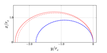
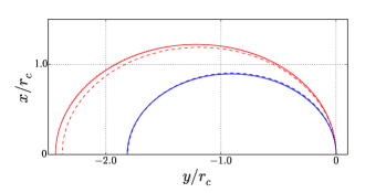
Figure 2: Trajectories of spin-orbit coupled holes, with $s=1$ in red, and $s=-1$ in blue. We use $\tilde{\gamma}_{3}=0.25$ and $\tilde{g}_{1}=1$ with an in plane magnetic field, $B_{||}=4$T. The Fermi energy is $\varepsilon_{F}=1.9$meV. The upper panel has a in plane magnetic field orientation $\phi=0$, while the lower panel has a field orientation $\phi=\pi/2$. We present the trajectories normalised with the cyclotron radii, with $r_{c}\approx l/2$. The dashed lines in the upper and lower panel have $B_{||}=0$T. Note that the change in the trajectory is very small. We note that the injection with velocity directed fully along $x$ does not correspond to $\theta_{i}=0$.

III Interference

The problem of interference in systems with large SOIs has been treated in detail for cylindrically symmetric systemsBladwell2017 . Like any interference problem, there are two trajectories (see Fig. 3), connecting the source located at the origin, $(0,0)$, to a detector located at $(0,l)$. These two paths are defined by injection angles $\pm\beta$, with

$$\cos\beta=\frac{l}{2r_{c,s}}$$ (17)

$$r_{c,s}=k_{F,s}/eB_{z}$$

Figure 3: The two trajectories of injection angle $\beta$ and $-\beta$.

Interference the arises from the difference between the phases of the two trajectories, with the semiclassical propagator defined as the sum over the two classically allowed paths,

$$K(\beta)\sim e^{i{\cal S}(\beta)}+e^{i{\cal S}(-\beta)}$$ (18)

with the phase ${\cal S}\propto\int{\bm{p}}\cdot d{\bm{l}}$, where $d{\bm{l}}$ is integrated along the path of the trajectories. In a typical TMF setup, the source and detector are of some finite aperture, with the Huygens Kernel, Eq. (18) averaged over this apertureBladwell2017 .

Evaluation of the phase is treated analogously to the cylindrically symmetric case. The canonical is related to the kinematic momentum and the vector potential by ${\bm{p}}=m{\bm{v}}+e{\bm{A}}$, and the action is

$${\cal S}(\beta)=\int_{\delta S}\left(m{\bm{v}}+e{\bm{A}}\right)\cdot d{\bm{l}}$$ (19)

where ${\bm{v}}$, ${\bm{A}}$, $d{\bm{l}}$ and the path, $\delta S$, are dependent on $\tilde{g}_{1}\mu_{B}B_{||}$. Using the previously determined equations of motion, Eqs. (II) and (II), the phase integral, Eq. (19) can converted into an integral over the running angle,

$${\cal S}(\beta)=eB_{z}\int_{\theta_{i}}^{\theta}\left(\left(\frac{dx}{d\theta^{\prime}}\right)^{2}+\left(\frac{dy}{d\theta^{\prime}}\right)^{2}-x\frac{dy}{d\theta^{\prime}}\right)d{\theta^{\prime}}$$ (20)

The relationship between the physical injection angle $\beta$ and $\theta_{i}$ is presented in Eq. (16). We must also determine $\theta$ in terms of $\beta$.

The trajectory from the source to the detector is, in terms of the running angle, from $\theta_{i}$ to $\theta$. This corresponds to the spatial positions $(0,0)$ and $(0,l)$ respectively. From Eq. (II) we have

$$x=0= \frac{k_{s}}{\omega_{c}m}\big{\{}(\sin\theta_{i}+\sin\theta)$$

$$+s\frac{\tilde{g}_{1}\mu_{B}B_{||}}{4}\left[\sin(2\theta-\varphi)-\sin(2\theta_{i}-\varphi)\right]\big{\}}.$$

We have restricted ourselves to a first order expansion in $\tilde{g}_{1}\mu_{B}B_{||}$ when performing the integration of Eq. (II). The trajectory deviates only minimally from the arc of a circle (see Fig. 2), and we can reasonably employ the approximation $\theta\approx\pi-\theta_{i}$ for the $\tilde{g}_{1}\mu_{B}B_{||}$ dependent terms. With this approximation, solving Eq. (III) we obtain

$$\theta\approx\pi-\theta_{i}-{s\tilde{g}_{1}\mu_{B}B_{||}}\sin\theta_{i}\cos\varphi$$ (22)

Finally, this can be expressed in terms of the injection angle, $\beta$ using Eq. (16), to obtain the integration limits for Eq. (20) in terms of $\beta$.

Using these integration limits, integration of Eq. (20) yields

$$S(\beta)=\frac{k_{s}^{2}}{2eB}\Big{\{}\pi-2\beta+\sin 2\beta+\zeta$$

$$-s{\tilde{g}_{1}}\mu_{B}B_{||}\sin\beta(1-\cos 2\beta)\cos\varphi\Big{\}}$$ (23)

$$\zeta={\tilde{g}_{1}}\mu_{B}B_{||}\Big{\{}\sin\varphi-\cos 2\beta\sin\varphi+\sin\varphi(\cos\beta+\frac{1}{3}\cos^{3}\beta)$$

$$\cos\varphi(\cos\beta+\frac{1}{3}\cos^{3}\beta)\Big{\}}$$

For $-\beta$ injection angles, we take $\beta\rightarrow-\beta$. We have introduced here $\zeta$ which contains the phase terms that do not contribute any net phase difference, that are symmetric for $\beta\rightarrow-\beta$. According to Eq. (18), we then have

$$K(\beta)\sim e^{i{\cal S}(\beta)}+e^{i{\cal S}(-\beta)}$$ (24)

$$\sim\sin\Big{[}\frac{k_{s}^{2}}{2eB}\Big{(}2\beta-\sin 2\beta$$

$$+s{\tilde{g}_{1}}\mu_{B}B_{||}\sin\beta(1-\cos 2\beta)\cos\varphi\Big{)}+\frac{\pi}{4}\Big{]}$$

The additional factor of $\pi/4$ arises due to the caustic for the $-\beta$ pathBladwell2017 . The third line of Eq. (18), which is linear in $\tilde{g}_{1}\mu_{B}B_{||}$, represents the “emergent phase contribution”, and is the first major result of this work. This term is particularly remarkable, since the classical trajectories have no first order dependence on $\tilde{g}_{1}\mu_{B}B_{||}$. For quantum (Shubnikov de Haas) oscillations, the integral is over the entire Fermi surface, and this term vanishes. Thus it is peculiar to the particular geometry of TMF, which defines the angle, $\varphi$ between the in plane magnetic field and the injector.

It is instructive to examine the variation in the interference fringe separation due to the application of the in magnetic plane field, expanding for small $\beta$. For small $\beta$, according to Eq. (III),

$$\beta\approx\sqrt{\frac{2r_{c,s}-l}{r_{c,s}}}=\sqrt{\frac{y}{r_{c,s}}}$$ (25)

Here $y=2r_{c,s}-l$ is the detuning from the classically forbidden region. For small $\beta$, Eq. (III) becomes

$${\cal S}\approx\frac{2}{3}\nu_{s}\left(\frac{y}{r_{c}}\right)^{\frac{3}{2}}\left(1+s\frac{3}{2}\tilde{g}_{1}\mu_{B}B_{||}\cos\varphi\right)$$ (26)

And from Eq. (III), we find a characteristic spacing of the interference fringes to be

$$\frac{\delta B}{B}\approx\frac{2.2}{2\nu^{\frac{2}{3}}}\left(1-s\tilde{g}_{1}\mu_{B}B_{||}\cos\varphi\right)$$ (27)

where $\delta B$ is the fringe spacing. This provides a method of determining the strength of the secondary spin orbit interaction. As can be seen in Fig. 4, even for the first interference fringe, there is a measurable shift. While there is no direct enhancement, the strength of the $\tilde{g}_{1}\mu_{B}B_{||}\sim 0.1\varepsilon_{F}$ at fields of a few Tesla in hole systems. Recent TMF experiments have resolved a single interference fringe for the low field peakRokhinson2004 ; Lo2017 , which would sufficient for the determination of $\tilde{g}_{1}\mu_{B}B_{||}$.

The remaining elements of the Huygen’s kernel are unchanged cyclindrically symmetric case. As was detailed in Ref. [Bladwell2017 ], the asymptotic form of the Huygen’s kernelcan be related to the Airy function. Employing the same reasoning, from Eqs. (III) and (26), we obtain,

$$K_{s}= e^{i\frac{\pi(\nu_{s}-1-n)}{2}}\frac{\nu_{s}^{2/3}}{2\sqrt{2}r_{cs}}\times$$

$$\left[(\sigma_{z}-is\sigma_{x})Ai(\overline{y}_{s})+\frac{n}{\nu_{s}^{1/3}}Ai^{\prime}(\overline{y}_{s})\right]\ .$$

Here $\overline{y}=y\nu_{s}^{2/3}\left(1+s\tilde{g}_{1}\mu_{B}B_{||}\cos\varphi\right)/r_{c}$. We present plots of the resulting interference spectrum in Fig. 4 with point-like sources and detectors, for both the classical form of the Huygen’s kernel, and Eq. (III). We stress that this semi-classical approach employed is only valid if $\nu_{s}\gg 1$. For typical experimental systems, $\nu_{s}>30$.

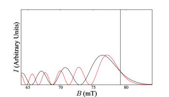
Figure 4: Interference pattern calculated for point-like source and detector from Eq. (III). We use $l=1500$nm, $k_{F}=0.107\times 10^{-1}$nm^-1 with a Rashba splitting $\tilde{\gamma}_{3}=0.3\varepsilon_{F}$, and $\tilde{g}_{1}\mu_{B}B_{||}=0.15\varepsilon_{F}$, corresponding to $B_{||}\sim 4-5$T for $\tilde{g}_{1}=1$ and $\varepsilon_{F}\approx 2$meV. For clarity we present only a single spin state. The Interference spectrum is calculated from Eq. (III), with Black vertical line indicates the location of the classical cutoff. Red (black) plots have in-plane field with $\varphi=\pi$ ($\varphi=0$)

IV Discussion

In real systems, the source and detector have finite size and can influence the observed interference pattern. Typically experimental devices use quantum point contacts, which consist of a narrow channel connecting a reservoir to the 2DHG. These have some characteristic width, $w$, and can be modelled by standing waves in the $y$ direction,

$$\psi_{s} \propto \chi_{s}\sin\left(\frac{\pi y}{w}\right)\ \ \ \ \ \ \ \ \ \ \ \ 0<y<w$$

$$\psi_{d} \propto \chi_{d}\sin\left(\frac{\pi(y-L)}{w}\right)\ \ \ L<y<L+w\ .$$ (29)

where $w$ is the width of the channel, and $\chi_{s}$ and $\chi_{d}$ are the eigenspinors at the source and detector respectivelyBladwell2017 . The exit width, $w$, is imposed by the lithographic geometry of the QPCMolemkamp1990 , however can vary depending on the conductance. We consider a hole gas with a density, $n=1.85\ 10^{11}cm^{-2}$, and corresponding Fermi momentum, $k_{F}=0.107nm^{-1}$. With a Rashba splitting of $\tilde{\gamma}_{3}=0.2\varepsilon_{F}$, the smaller spin-split Fermi momentum will be $k_{-}=0.096nm^{-1}$ ($\lambda\approx 66nm$) and the larger Fermi momentum $k_{+}=0.118nm^{-1}$ ($\lambda\approx 53nm$). The distance between the source and the detector is $L=1500nm$. The corresponding magnetic field at the classical edge of the bright region for $k_{-}$ is $B_{-}=77mT$, while for $k_{+}$, $B_{+}=94mT$. We will start by considering a QPC of width $w=150$nm, which we note corresponds to the lithographic width of the device of Ref Rokhinson2004 . The resulting focusing spectrum is presented in Fig. 5. While interference fringes are still visible, they are suppressed, and the additional phase contribution manifests as a suppression or enhancement of the spin-split focusing peaks. We note that this experimental signature is similar to that typically attributed to polarisation in the QPCsReynoso2007 .

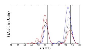
Figure 5: Interference patterns versus $\tilde{g}_{1}\mu_{B}B_{||}$, with range $-0.1<\tilde{g}_{1}\mu_{B}B_{||}<0.1$, with $\varphi=0$. Here $l=1500$nm, $w=150$nm. Positive $\tilde{g}_{1}\mu_{B}B_{x}$ is presented in red, while negative $\tilde{g}_{1}\mu_{B}B_{x}$ are in blue. The $B_{x}=0$ TMF spectrum is solid black curve. Vertical black lines indicate the location of the classical maximum, $B_{focusing}=2\hbar k_{s}/el$.

In summary, we have employed Huygen’s principle to determine quantum interference for systems with asymmetrical Fermi surfaces. While in this work we focus on a specific case of an in-plane magnetic field in combination with a Rashba spin-orbit interaction, the method employed is general. We have predicted an emergent phase contribution, linear in the applied in plane magnetic field, despite there being no first order changes to the classical trajectories. This emergent phase term significantly alters the interference spectrum of TMF. We propose that this could be used to measure the in plane $g$ factor.

V Acknowledgements

We thank Alex Hamilton, Dmitry Misarev, Harley Scammell and Matthew Rendell for their helpful discussions. SSRB acknowledges the support of the Australian Postgraduate Award. This research was partially supported by the Australian Research Council Centre of Excellence in Future Low-Energy Electronics Technologies (project number CE170100039) and funded by the Australian Government.

References

- (1) Yu. V. Sharvin, Zh. Eksp. Teor. Fiz. 48, 984 (1965) [Sov. Phys. JETP 21, 655 (1965)].
- (2) Yu. V. Sharvin and L. M. Fisher, Pis’ma Zh. Exp. Teor. Fiz. 1, 54 (1969) [Sov. Phys. JETP Letters 1, 152 (1965)].
- (3) V. S. Tsoi, Pis’ma. Zh. Exp. Teor. Fiz. 19, 114 (1974) [Sov. Phys. JETP Letters 19, 70 (1974)].
- (4) V. S. Tsoi, J. Bass, P. Wyder, Rev. Mod. Phys. 71, 1641 (1999).
- (5) H. van Houten, C. W. J. Beenakker, J. G. Williamson, M. E I Broekaart, P. H. M . van Loosdrecht, B. J. van Wees, J. E. Mooij, C. T. Foxon, and J. J. Harris, Phys. Rev. B.39, 8556 (1989).
- (6) T. Taychatanapat, K. Watanabe, T. Taniguchi, and P. Jarillo-Herrero, Nat. Phys. 9, 225 (2013).
- (7) L. P. Rokhinson, V Larkina, Y. B. Lyanda-Geller, L. N. Pfeiffer, K. W. West, Phys. Rev. Lett. 93, 146601 (2004).
- (8) L. P. Rokhinson, L. N. Pfeiffer, and K. W. West, Phys. Rev. Lett. 96, 156602 (2006).
- (9) G. Usaj and C. A. Balseiro, Phys. Rev. B 70, 041301 (2004).
- (10) U. Zülicke, J. Bolte, and R. Winkler, New J. Phys. 9, 355 (2007).
- (11) S. Bladwell and O. P. Sushkov, Phys. Rev. B, 92, 235416 (2015); S. Bladwell and O. P. Sushkov, Phys. Rev. B 95, 159901(E) (2017)
- (12) A. Reynoso, G. Usaj, and C. A. Balseiro, Phys. Rev. B 75, 085321 (2007).
- (13) S. Bladwell and O. P. Sushkov, Phys. Rev. B 96, 035413 (2017).
- (14) Y. A. Bychkov and E. I. Rashba, J. Phys. C 17, 6039 (1984)
- (15) Shun-Tsung Lo, Chin-Hung Chen, Ju-Chun Fan, L. W. Smith, G. L. Creeth, Che-Wei Chang, M. Pepper, J. P. Griffiths, I. Farrer, H. E. Beere, G. A. C. Jones, D. A. Ritchie and Tse-Ming Chen, Nat. Comms. 8, 15997 (2017)
- (16) R. Winkler, 2003, Spin-orbit Coupling Effects in Two-Dimensional Electron and Hole Systems, (Springer, New York)
- (17) T. Li, L. A. Yeoh, A. Srinivasan, O. Klochan, D. A. Ritchie, M. Y. Simmons, O. P. Sushkov, and A. R. Hamilton, Phys. Rev. B 93, 205424 (2016)
- (18) D. S. Miserev and O. P. Sushkov, Phys. Rev. B 95, 085431 (2017)
- (19) P. J. Simmonds, F. Sfigakisa, H. E. Beere, D. A. Ritchie, M. Pepper, D. Anderson, and G. A. C. Jones, Appl. Phys. Lett. 92, 152108 (2008)
- (20) L. W. Molenkamp, A. A. M. Staring, C. W. J. Beenakker, R. Eppenga, C. E. Timmering, J. G. Williamson, C. J. P. M. Harmans, and C. T. Foxon, Phys. Rev. B 41, 1274 (1990)
- (21) A. Reynoso, Gonzalo Usaj, and C. A. Balseiro, Phys. Rev. B 75, 085321 (2007)