Photon correlations in both time and frequency

1 Introduction

Similarly to Satie’s understanding of music as “measuring sound”, Quantum Optics can be understood as the science of measuring photon correlations. This led to one of the most recent revolutions concerning our understanding of light, establishing among other things that coherence is not a feature of monochromaticity but a quality of photon correlators to factorize. Most of the field has concerned itself with time-resolved photon correlations but to get a comprehensive picture, one should also describe correlations in other variables (polarization, position, etc.) One is particularly important in any dynamical system: energy. Being a quantum mechanical problem, and since energy is $\hbar$ times the frequency, this brings head on the problem of conjugate variables and the uncertainty principle [1]. Of particular interest is Resonance Fluorescence (driving resonantly a two-level system), whose spectral shape—the Mollow triplet—posed the question of peak-to-peak correlations in the early days of the field [2]. Thanks to a new technique to compute exactly frequency- and time-resolved photon correlations [3], we have been able to provide the full landscape of $N$-photon correlations from nontrivial systems [4]. This has been experimentally measured [5] and found to be in excellent agreement with the theoretical predictions. Such an approach reveals a new class of transitions, the leapfrog processes, that involve $N$-photon transitions over $N-1$ manifolds of excitation. This makes for strongly quantum correlated emission [6]. Intercepting (e.g., by filtering) such degenerate leapfrog transitions allows to realize a regime of pure $N$-photon emission [6, 7]. The landscape of correlation however extends far beyond the case of degenerate photons, and a rich hyperspace of photon correlations exist at the “photon-bundle” level [8], where one can correlate not simply photons but groups, or “bundles” of them. This should allow such a system to service a rich class of heralded $N$-photon sources. Such sources, if realized, would clearly have strong implications for quantum spectroscopy (by exciting optical targets with this new type of quantum light) [9, 10]. In this text, written at the occasion of the METANANO 2018 in Sochi, we present some illustrative and original results, highlighting the temporal aspect on the one hand (for some fixed frequency) and the frequency aspect on the other hand (for some fixed time, usually, the case of coincidences, as this is the case which usually draws the greatest attention). While the formalism [3] covers these two aspects simultaneously, it is helpful and/or enlightening to look at them separately. Since hastily reading observers may otherwise get a wrong impression on the generality of the results, we also present a case where correlations in both time and frequency are displayed. To also emphasize that the method is exact and see how it compares with previous theories, that were not, we show explicit calculations for both cases.

2 Correlations in time

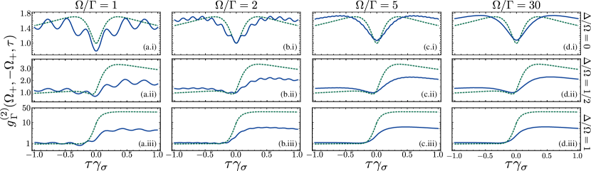
Figure 1: Comparison between the filtered correlations from the side peaks of the Mollow triplet, as obtained exactly through the sensing method (solid blue) and approximately as in Ref. [11] (dashed green). The driving intensity $\Omega$ is varied from panels (a) to (d), and detuning between laser and emitter from panels (i) to (iii). Oscillations are lost in the approximation and the bunching peak associated to photon heralding is overestimated. Parameters: $\Gamma/\gamma_{\sigma}=10$ ($\gamma_{\sigma}$ the emitter decay rate) and rest as shown.

Photon correlations are typically measured as a function of time-delay between successive photons. With two photons, this yields the quantity $g^{(2)}(\tau)$ (the so-called $2^{\mathrm{nd}}$ order correlation function). The frequency-resolved version interposes filters in front of the detectors and the quantity becomes $g^{(2)}_{\Gamma}(\omega_{1},\omega_{2},\tau)$ (here with the same frequency window $\Gamma$ for both detectors, which needs not be the case, see, e.g., Fig. 5 of Ref [12]). The formal expression to compute was obtained exactly in the 80s, providing a great result of photo-detection theory, but the actual computation proved too complex and approximations had to be introduced. Typically, following the fruitful dressed state picture, auxiliary states are used and correlations between them computed as an approximation. We will consider the case of correlations between the side peaks of the Mollow triplet, and compare the results from Ref. [11](dashed green in Fig. 1), which rely on this approximation, with our results (solid blue), which are numerically exact. Overall, Physics is safe. The approximation is not exact and can even fail qualitatively (most notably, it does not depend on driving and misses oscillations at low driving) but the basic behaviour is well captured and fairly accurate at high-driving and resonance (the perfect agreement with experimental data is maybe less satisfactory [11, 13] but fitting the less accurate model with free parameters can achieve that). The main limitation however lies elsewhere. Correlations are pinned to peaks emission in this approximation, which motivates its form in the first place. However, much more interesting correlations are to be found away from the peaks.

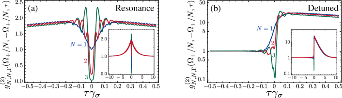
Figure 2: Two $N$-photon time cross-correlations at frequencies $\pm\Omega_{+}/N$ (on both sides of the central peak of the Mollow triplet with $\Omega_{+}$ its splitting) for $N=1$ (blue lines), $2$ (red lines) and $3$ (green lines). (a) Resonant excitation and (b) detuned excitation (insets shown longer times). The detuning in (b) is $\omega_{\sigma}=200\gamma_{\sigma}$. For all cases $\Omega_{+}=300\gamma_{\sigma}$ and $\Gamma=40\gamma_{\sigma}$, which maximizes the superpoissonian peak.

Figure 2 shows $N$-photon correlations at the frequencies $\pm\Omega_{+}/N$ for $N=1$ (in blue, cross-correlations of two single-photons from the side peaks, as in Fig. 1), $N=2$ (in red, cross-correlations of two two-photon states halfway between the central and side peaks) and $N=3$ (cross-correlations of two three-photon states at one-third of the frequency between the central and side peaks). Not only do we now access frequencies previously out of reach, but we also consider correlations between bundles ($N$-photon states), introducing the quantity $g_{{n_{1}},{n_{2}},\Gamma}^{(2)}(\omega_{1},\omega_{2})\equiv{\langle{:}\Pi_{\mu=1}^{2}{a^{\dagger}}^{n_{\mu}}(\omega_{\mu})a^{n_{\mu}}(\omega_{\mu}){:}\rangle}/(\Pi_{\mu=1}^{2}\langle{a^{\dagger}}^{n_{\mu}}(\omega_{\mu})a^{n_{\mu}}(\omega_{\mu})\rangle)$ (with $a(\omega)$ the annihilation operator of a photon of frequency $\omega$ and : normal ordering) that correlates a $n_{1}$-photon bundle of frequency $\omega_{1}$ with a $n_{2}$-photon bundle of frequency $\omega_{2}$ both in frequency windows of width $\Gamma$ (this can be generalized to different frequency windows [8]). While single-photon correlations become not particularly noteworthy, we see here that the same phenomenology is transported to photon bundles. One can indeed recognize in the insets of Fig. 2(b) the familiar profiles of photon heralding, but at the $N$-photon level. These results are thus not only exact, but also unique.

3 Correlations in frequency

The correlation spectrum in frequency is probably the most conceptually striking, as it brings a new dimension to the problem. It turns a number, $g^{(2)}(0)$, into a picture, as shown in Fig. 3. Panel (a) correlates two photons of arbitrary frequencies, and is the case already measured experimentally [5]. The antidiagonal red lines are “leapfrog processes” and show regions where the system tends to emit photons in pairs. Since we have amply discussed two-photon spectra in previous works [4], we turn directly to the even greater family of two $N$-photon bundles correlation spectra. Panels (b) and (c) show correlations between two-photon and three-photon bundles, respectively, here at resonance. In each case, the structure of the correlation spectrum can be easily understood from leapfrog transitions, shown in insets $i$–$iii$ along with, in panels (d)–(f), the traces they imprint in the correlation spectra, with corresponding color codes. Note how case $iii$, for instance, involves six photons, in a plethora of photon emissions of various orders, leading to a crowded landscape with myriads of leapfrogs. Nevertheless, these are all clearly resolved in $g^{(2)}_{3,3}$ and understood in simple terms. Such correlated emission can power devices.

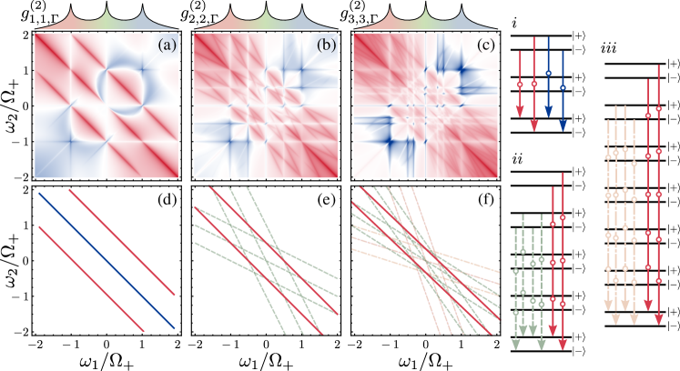
Figure 3: Landscape of two $N$-photon bundle correlations for (a) $N=1$, (b) $N=2$ and (c) $N=3$, with red corresponding to bunching, blue antibunching and white no correlations. The structure, sketched in panels (d)–(f), comes from leapfrog transitions, shown in insets $i$–$iii$ with corresponding colors. The structure in (d) is also present in (b) and (c) and that in (e) is also present in (c) (and so on to higher orders). Parameters: $\Omega_{+}=300\gamma_{\sigma}$, laser-emitter detuning $\omega_{\sigma}=200\gamma_{\sigma}$ and filtering window $\Gamma=5\gamma_{\sigma}$.

4 Correlations in both time and frequency

At this stage, it is clear that we have jointly considered correlations in both time and frequency. We will let an image speak a thousand words, with Fig. 4 showing photon correlations simultaneously in time and frequency, in a 3D space (that we have projected on two planes for clarity). Heisenberg uncertainties are satisfied through $\Gamma$. There is no numerical difficulty in getting these results, which have all been obtained with a high-level programming language on a middle-end personal laptop in time of the order of a few minutes. The only difficulty that arises is not in obtaining the data in the first place, but in processing and displaying it, as this starts to provide a fairly comprehensive picture of a nontrivial quantum mechanical system.

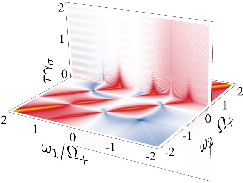
Figure 4: Two-photon correlations $g_{\Gamma}^{(2)}(\omega_{1},\omega_{2},\tau)$ from the Mollow triplet with a cut of time correlations at $\omega_{2}=\Omega_{+}/2$, showing how leapfrog processes imprint strong correlations in time along with the peaks emission. Of course the cut could be taken anywhere in the two-photon spectrum. Parameters: $\Gamma=5\gamma_{\sigma}$, $\Omega=87\gamma_{\sigma}$, $\Omega_{+}=174\gamma_{\sigma}$ and driving at resonance.

5 Conclusions

We have summarized the main results that follow from our theory of frequency- and time-resolved photon correlations [3], which provides exact computations in nontrivial systems. We illustrated the theory with original results as interesting cases can be picked up from the endless configurations that abound in any quantum optical system. In particular, we have compared our exact results with previous approximations, upgraded correlations to the case of bundles as otherwise no clear physical picture emerge, highlighted the interest of measuring away from the peaks in rich landscapes of correlations and emphasized the joint time and frequency aspect of our theory. Such results can power a new class of optical devices, out of which we foresee heralded $N$-photon emitters as the most decisive breakthrough for today’s photonics.

References

References

- [1] E. del Valle, J. C. L. Carreño, F. P. Laussy, arXiv:1802.04540 (2018).
- [2] C. N. Cohen-Tannoudji, S. Reynaud, J. Phys. B.: At. Mol. Phys. 10, 345 (1977).
- [3] E. del Valle, et al., Phys. Rev. Lett. 109, 183601 (2012).
- [4] A. González-Tudela, et al., New J. Phys. 15, 033036 (2013).
- [5] M. Peiris, et al., Phys. Rev. B 91, 195125 (2015).
- [6] C. Sánchez Muñoz, et al., Nat. Photon. 8, 550 (2014).
- [7] C. Sánchez Muñoz, et al., Optica 5, 14 (2018).
- [8] J. C. López Carreño, E. del Valle, F. P. Laussy, Laser Photon. Rev. 11, 201700090 (2017).
- [9] J. C. López Carreño, et al., Phys. Rev. Lett. 115, 196402 (2015).
- [10] J. C. López Carreño, F. P. Laussy, Phys. Rev. A 94, 063825 (2016).
- [11] C. A. Schrama, et al., Phys. Rev. A 45, 8045 (1992).
- [12] A. González-Tudela, E. del Valle, F. P. Laussy, Phys. Rev. A 91, 043807 (2015).
- [13] A. Ulhaq, et al., Nat. Photon. 6, 238 (2012).