A shiny update to an old experiment game

Abstract

Games can be a powerful tool for learning about statistical methodology. Effective game design involves a fine balance between caricature and realism, to simultaneously illustrate salient concepts in a controlled setting and serve as a testament to real-world applicability. Striking that balance is particularly challenging in response surface and design domains, where real-world scenarios often play out over long time scales, during which theories are revised, model and inferential techniques are improved, and knowledge is updated. Here I present a game, borrowing liberally from one first played over forty years ago, that attempts to achieve that balance while reinforcing a cascade of topics in modern nonparametric response surfaces, sequential design and optimization. The game embeds a blackbox simulation within a shiny app whose interface is designed to simulate a realistic information-availability setting, while offering a stimulating, competitive environment wherein students can try out new methodology, and ultimately appreciate its power and limitations. Interface, rules, timing with course material, and evaluation are described, along with a “case study” involving a cohort of students at Virginia Tech.

Key words: response surface, computer experiment, experimental design, Bayesian optimization, input sensitivity, teaching game

.

1 The setting

In-class games are a common way to encourage learning—to interject some fun and build intuition in an seemingly esoteric, or tedious technical landscape. A good game could be fundamental to retaining students, say in introductory statistics. One fine example uses chocolate chip cookies to illustrate aspects of sampling distributions (Lee,, 2007). The long arc of an out-of-class game played over an entire semester is attempted rather less frequently. However for some topics, like experimental design and response surface optimization, that setting is quite natural: real-life applications play out on longer temporal scales, and in an inherently dynamic landscape. In this article I present such a game, designed to simulate a real-world setting that students might encounter on internship, which was played during a graduate course I recently gave at Virginia Tech. The game is an update of one first played over forty years ago (Mead and Freeman,, 1973).

Mead and Freeman,’s game was ahead of its time. Today, few are aware of the contribution. Although it is cited prominently in Box and Draper, (1987), which is how I found it, that is one of just eight references in the literature. Perhaps this is because, for many decades (70s-90s, say) the setup of the game, requiring a custom computing environment with student access, was hard to replicate. Today, with R/CRAN (R Core Team,, 2017) implementation and shiny (Chang et al.,, 2017) web interfaces, barriers have come way down.

The original game involves blackbox evaluation of agricultural yield as a function of six nutrient levels, borrowed from Nelder, (1966) and reproduced in R as follows.

yield <- function(N, P, K, Na, Ca, Mg)
{
  l1 <- 0.015 + 0.0005*N + 0.001*P + 1/((N+5)*(P+2)) + 0.001*K + 0.1/(K+2)
  l2 <- 0.001*((2 + K + 0.5*Na)/(Ca+1)) + 0.004*((Ca+1)/(2 + K + 0.5*Na))
  l3 <- 0.02/(Mg+1)
  return(1/(l1 + l2 + l3))
}

Players obtain noisy yield evaluations, due to additive block and plot-within-block (Gaussian) effects, with the ultimate goal of maximizing yield. There are five computer sessions (simulating crop years). Multiple experiments can be undertaken in a single session but strategies can only be revised between sessions. My updated version still focuses on maximizing yield through a series of runs, and its inaugural run involved a yield form very similar to the one coded above. The specifics are detailed in Section 2. But the environment no longer considers blocks and plots.

My revisions to the game are primarily motivated by modern technology/application, and a desire to teach a more sophisticated statistical toolkit. Classical response surface methods and design emphasize low degree (first- and second-order) linear modeling. The resulting steepest ascent and ridge analyses (see, e.g., Box and Draper,, 1987; Myers et al.,, 2016) enjoy a high degree of analytical tractability. Many relevant calculations can either be performed by hand, or with a graphing calculator. Yet such conveniences offer negligible advantage in modern applications demanding facilities that, historically, would have been considered supercomputing but are now simply routine numerics. Two prominent examples are information technology/e-commerce and computer simulation experiments. Modern response surface methods in those domains borrow heavily from geostatistics and machine learning with Gaussian processes, deep neural networks, and regression and classification trees. Sequential design strategies like expected improvement (Jones et al.,, 1998) promise a more modular approach to (so-called Bayesian) optimization, allowing fancy models to be swapped in and out, and a degree of human-free automation with light coding. My teaching and research philosophy favors modularity in implementation, and the game was in part conceived to reinforce those aspects in practice.

Several aspects of the new game setup emphasize friendly competition as a means of enhancing the learning arena. Exploring a diverse, state-of-the-art, toolkit benefits from sandboxing aspects of game play, but the superlative nature of the goal—of optimizing yield—organically encourages students to adapt and improve over time. Relative benchmarks also enhance the sense of realism, albeit through somewhat artificial means. At the same time, it remains important that students feel compelled engage with the game in a way that is advantageous pedagogically, which for some could come at the expense of winning. Toward that end, Section 3 covers player benchmarking, timing of methodology with lecture material, and an assessment strategy designed to encourage regular engagement and the deployment of a wealth of tools. Some results from a real run of the game at Virginia Tech are provided. Section 4 concludes with lessons learned and ideas for future variations. An online supplement includes a suite of supporting codes and other materials.

2 Game design

The core of game play is facilitated by an R shiny app, shown in Figure 1, which serves as both a multi-player portal and an interface to the back-end database of player(s) records. An Rmarkdown document, yield.Rmd, provided with the supplementary material, compiles a full set of instructions on how to use the app, the rules of the game, and some suggestions about strategy. An HTML rendering of that document is provided at http://bobby.gramacy.com/teaching/rsm/yield.html. The salient details follow.

2.1 Using the shiny app

Since all game players use the same app, interaction begins with a “logging in” phase. In advance of opening the game, I asked each player to provide me with their initials (2–4 characters) and a four-digit secret PIN, the combination of which comprises of the login token. Logging in involves providing “url?token” in the browser search bar. In Figure 1 the URL points to a local shiny server, and the token is “rbg4036”, a combination of my initials (I played the game too) and my office number, 403G.

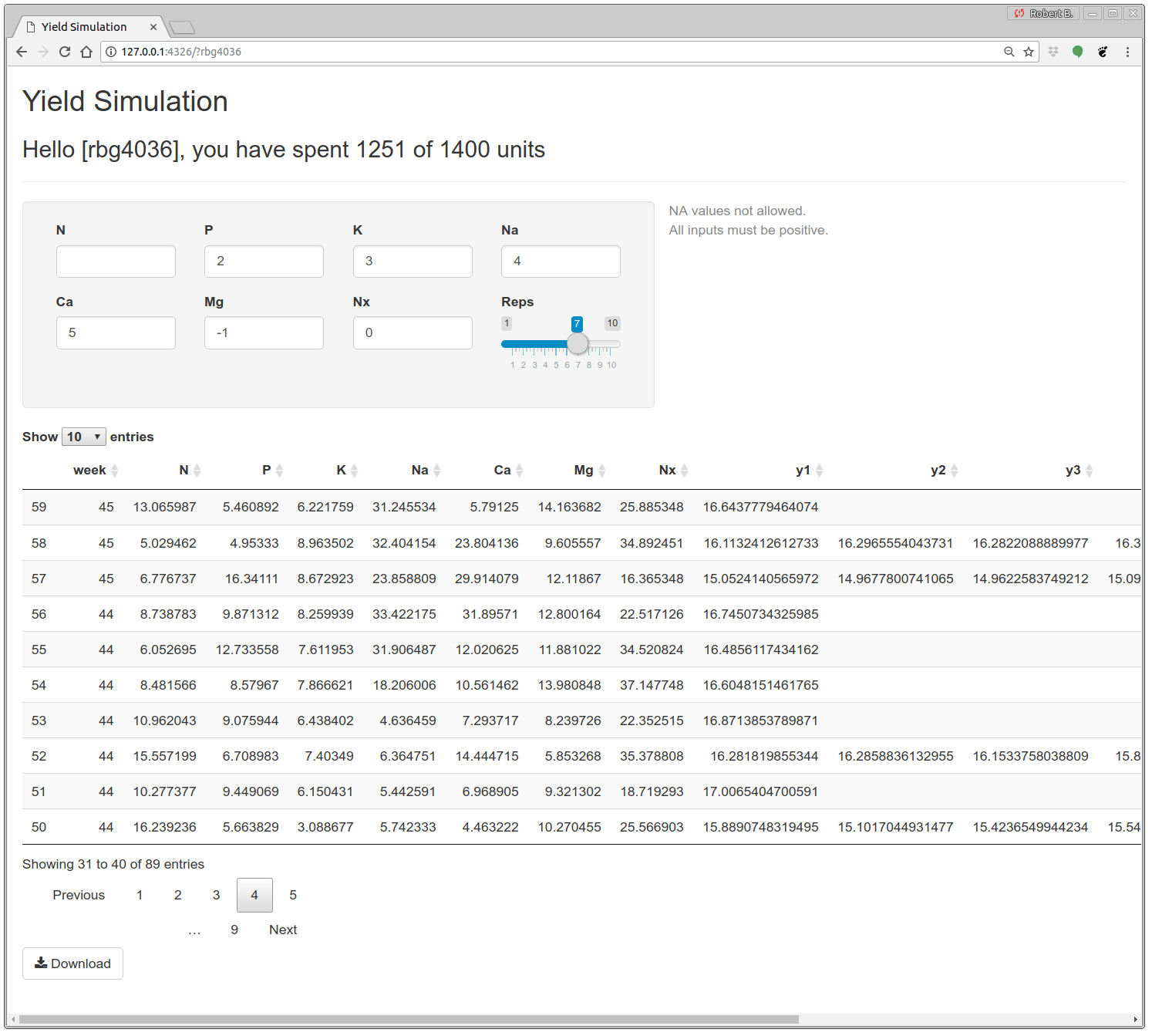
Figure 1: An interactive yield simulation session. User rbg4036 may inspect the run budget, perform new runs (if budget remains), browse historical runs, or download a text file.

Once logged in, the player is presented with three blocks of game content. A greeting block provides details on spent and total budget for experimental runs. How the budget works, costs of runs, etc., is discussed in detail in Section 2.2. As long as the player has not fully spent, or over-spent, their budget, new runs may be performed, via the second block on the page. Here, the player enters the coordinates of the next run. Until all fields are populated with valid (positive, non-empty) values, helpful error messages appear on the right. The last input, which is a slider, indicates the number of replicates desired—again discussed in more detail shortly. Once all entries are valid, the error messages are replaced by a “Run” button and a warning that there are no do-overs.

Performing a run causes the table in the final block of the page to be updated, with the week, inputs, and outputs of the new run appearing at the top of the table. The primary purpose of the table is to provide visual confirmation that the run has been successfully stored in the player’s database file. Buttons are provided to aid in browsing, however this is not intended as the main data-access vehicle. A “Download” button at the bottom creates a text file which can be saved via browser support—usually into the ~/Downloads directory. Empty output fields are converted to NAs in the downloaded file.

The appendix contains some details about the backend of the shiny app, including special considerations required for hosting in the cloud, say on shinyapps.io.

2.2 Rules, startup and twists

Players are encouraged to collaborate on strategy, and the development of relevant mathematical calculations, but they may not share code or data. They start with a database containing an identical design of seven inputs, each with five replicate responses whose noise structure is explained momentarily. Students were introduced to the game in the fifth week (game week zero), and could perform their first runs in the sixth week of a 15-week semester. Including Thanksgiving and final exam weeks tallies thirteen weeks of game play.

In each week, including week zero, students accrue 100 playing units to spend on runs, with full roll-over from previous weeks. The cost structure for runs favors replicates. Obtaining the first replicate costs ten units. Replicates two through four cost an additional three units each; five through seven cost two, and eight through ten cost one each. As long as a player’s account is in the black (i.e., positive balance), s/he can perform a new run with as many replicates as desired, up to the limit of ten. If performing that run causes the balance to be zero, or negative, future runs will not be allowed (the run box on the app disappears) until the following week, after 100 new units are added.

Replication is important for two game “twists” designed to encourage players to think about signal-to-noise trade-offs, and to nudge them to spend units regularly, rather than save them all until the end of the semester. The first is that players are told that the variance of the additive noise on yield simulations is changing weekly, following a smooth process in time, and that they will need to provide an estimate of that variance over time for their final report. They are further warned that the variance may be increasing, effectively devaluing unused units. In fact the variance in week $w$ followed a simple sinusoidal structure

$$\sigma^{2}(w)=0.1+0.05(\cos(2\pi(w-w_{s})/10)+1)\quad\quad\mbox{for starting week}\;w_{s},$$

which peaks in the first and tenth week. The second wrinkle is a seventh input, Nx, which is unrelated to the response. Students are not told that one of the inputs is useless, however the final writeup instructions ask for sensitivity analyses for the inputs, including main, partial dependence, and total effects.

3 Timing, outcomes and evaluation

The class was offered as a 6000-level seminar, which graduate students in statistics usually take after they’ve completed the bulk of their coursework requirements for a terminal degree (Masters or Ph.D.). Most students were, therefore, not novices in the core pillars of the course: linear and nonlinear regression, design, etc. But few had previously worked in an environment similar one synthesized by the game. Starting in the fifth week of the semester allowed for ramp-up on methodological training, giving students the chance to learn/review fundamentals like steepest ascent and ridge analyses (e.g., Myers et al.,, 2016, Chapters 5–6) before entering the game as players. Using R code provided in class, most students were able perform runs in the first two weeks that improved upon yields from week zero, while getting a feel for the system. In subsequent weeks, new methodology was introduced which students were expected to try in the game. Most students had not, previously, been exposed to these topics, which leverage nonparametric response surfaces. Conceptual and implementational hurdles were anticipated by a careful timing of training (first examples in lecture and homework) and testing (live, in the game) stages in the course development. Details on how game play tracks course material, cookie crumbs to “catch up” stragglers, and windows into game progress are provided below.

3.1 Subject progression and homeworks

Homeworks were assigned roughly every two weeks and each one, from the third onward, contained a problem on the game. Problem statements and solutions are provided with the supplementary material. The third homework was the the most prescriptive about what to do in the game. It instructed the student to fit a first-order model to the initial data set ($7\times 5$ runs) and determine which of the seven main effects were useful for describing variation in yield. In my own solution, only the first three were relevant, e.g., after a backwards step-wise selection procedure with BIC. Then, after reducing to a first order model having only those three components, they were asked to search for interactions. I found one.

With best fitted model in hand, students were asked to characterize a path of steepest ascent, and to obtain yield simulations along that path. This required determining values for the remaining (in my case four) inputs. No guidance was given here; I used a Latin hypercube sample, paired with six settings of the three active variables a short ways along the path of steepest ascent. Next, students were given several options about how to proceed, including a second-order ridge analysis, more exploration with space-filling designs, or more steepest ascent. In my own solution I did a bit of all three, and the result was a second-order fit to the data that had many relevant main effects, interactions, etc.

After the homework deadline, I released my solution so students could see what I did, and use it to “catch up” with other players during subsequent weeks. Then we transitioned to modern material involving Gaussian processes (GPs), presented from machine learning (Rasmussen and Williams,, 2006) and computer surrogate modeling (Santner et al.,, 2003) perspectives. Both communities evangelize the potential for fitted GP predictive surfaces to guide searches for global optima in blackbox functions. Machine learning researchers call this Bayesian optimization, whereas computer modelers call it surrogate-assisted optimization (however increasingly they are adopting the machine learning terminology). The simplest variation involves optimizing the fitted GP predictive mean equations (Booker et al.,, 1999), in lieu of working directly with locally winnowed input–output data pairs. The method of expected improvement (EI, Jones et al.,, 1998) and integrated variations (e.g., IECI, Gramacy and Lee,, 2011) were subsequently introduced to better balance exploration and exploitation by incorporating degrees of predictive variability (local to global), a hallmark of statistical decision-making. This family of nonparametric approaches were reinforced in three questions spanning three subsequent homeworks. Solutions were provided (after the due dates) as plug-n-play R scripts leveraging mature laGP subroutines (Gramacy,, 2016), converting a database file into a suggested new run without any additional human interaction.

As one example consider EI, which is based on the improvement: $I(x)=\max\{0,f^{\mathrm{min}}_{n}-Y(x)\}$. The quantity $f^{\mathrm{min}}_{n}$ is best value of the objective so far, and $Y(x)$ is a prediction of that objective as a function of the inputs $x$. Both are derived from the estimated response surface, and are thus random variables—a property inherited by $I(x)$. Although there are many variations in the literature, the most common setup simplifies to treat $f^{\mathrm{min}}_{n}$ as a deterministic quantity derived from minimizing mean predictive surface for $Y(x)$, and supposes that surface to be Gaussian. In such cases, as arises when training a GP on input-output pairs $(x_{1},y_{1}),\dots,(x_{n},y_{n})$, the distribution of $Y(x)$ is completely specified by $\mu_{n}(x)$ and $\sigma^{2}_{n}(x)$, which have closed form expressions. Integrating $I(x)$ over $Y(x)$ is also analytically tractable in that Gaussian setting, leading to the expected improvement (EI):

$$\mathbb{E}\{I(x)\}=(f^{n}_{\min}-\mu_{n}(x))\,\Phi\!\left(\frac{f^{n}_{\min}-\mu_{n}(x)}{\sigma_{n}(x)}\right)+\sigma_{n}(x)\,\phi\!\left(\frac{f^{n}_{\min}-\mu_{n}(x)}{\sigma_{n}(x)}\right),$$

where $\Phi$ and $\phi$ are the standard normal cdf and pdf, respectively. Notice how EI naturally balances exploitation, $\mu_{n}(x)$ below $f_{\min}^{n}$, and exploration, large $\sigma_{n}(x)$, which is key to automating iterations of search for local optima (by maximizing $\mathbb{E}\{I(x)\}$ over $x$).

Homework 5, provided in the supplementary material, asked students to try EI in the game. That homework was assigned in week 7 of game play, and variations were considered in subsequent homeworks/weeks. Although timing is difficult to pinpoint exactly, the students’ implementation of EI-like methods, and the scripts provided as catch-up after the due date (week 9, see, e.g., yield_gp_ei.R in the supplementary material), are responsible for much of the progress realized in latter weeks. For example student “mds”, who had relatively mediocre success with classical RSM tools, saw big improvements [see Figure 2] from employing these more sophisticated, but more easily automated, tools.

3.2 Leaderboard

In hopes that friendly competition would spur interest, I provided leaderboard-style views into players’ performance relative to one another, updated in real time. A live Rmarkdown script compiled four views into player progress for web viewing.

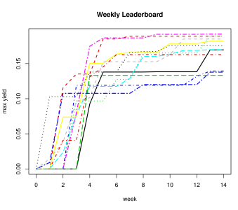
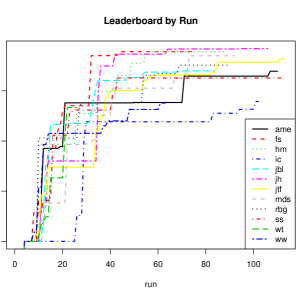
Figure 2: Two de-noised views into the real-time leaderboard during the final week of game play: best yield by week (left), and by run (right).

Two of those views, snapped during the final week of game play, are provided in Figure 2. On the $x$-axis is the week of game play (left panel) or the unique run number (right), and on the $y$-axis is a normalized yield response. Each player has a line in the plot, with color and type indicated by their initials (masking the pin). The responses shown have been de-noised in order to view pure progress, making normalization essential otherwise players would know the true mean value of their best noisy response. The two other views provided by the Rmarkdown script show “raw” versions of these same plots, on the original scale—these are not shown here.

Observe from the panel that about half of the progress is made in the first five weeks, spanning around forty runs. Students “jh” and “fs” made rapid progress. By contrast, “hm” ends up at the same place in the end, but with more steady increments. The leaderboard would seem to partition students into three classes, comprising of the top five, middle four, and lower four. Evidently, student “wt” gave up early and “ww” may have misjudged the appropriate balance of replicates versus unique runs. These students, while not having the strictly poorest overall performance in terms of max yield, received the lowest grades on the project. Their final writeup reinforced an erstwhile low engagement with many aspects of the competition, including a failure to capitalize on the “catch up” scripts provided as part of the homework keys. Finally, observe in the figure that my own strategy placed me fifth by these measures. I favored replication over unique runs in hopes of obtaining better main effects, sensitivity indices, and estimates of variance over time. Very few students picked up on the small asymptotic effect of Mg, commented on the potential useless of Nx, or picked up on periodic effects in the noise. Although all three were evident in my own solution, that’s perhaps because I knew in advance what to look for. Despite those caveats, students with the best yield results on the leaderboard had remarkably tight estimates for the optimal coordinates of the five “active” inputs, relative both to one another and to the truth.

4 Discussion

I have described a statistical optimization game updating a previous one in two senses. The first sense is that the game uses modern tools for implementation. Supplementary materials provide R code with support for a shiny app interface, cloud storage for instance-based hosting like shinyapps.io, and real-time views into progress via a leaderboard. Although the original version of the game was innovative, when introduced it was essentially unusable by others at the time owing to the nature of computing environments available in the early 1970s. The second update has to do with modern response surface methods. My re-casting of the game, and the homework problems from class which support it, emphasize a machine learning and computer surrogate modeling “hands-free” toolkit from the 21st century.

Upon reflection, the game perhaps could be revised to better emphasize these more modern tools. Students who made early progress on the leaderboard unfortunately realized diminishing returns from methodological upgrades developed later in the semester. In some sense, the had been “unlucky” in finding right answer “too early” to benefit from the modern tools. I recall an office hours session where one of the better students, “fs”, was somewhat distraught by lack of improvement in yield from his/her EI implementation. Eventually, I had no choice but to reveal that s/he had essentially “solved it” so that s/he could move productively on to other things. In future play I may opt for a multi-modal blackbox in order to keep students engaged, and to demonstrate the explorative value that comes from EI and IECI-like heuristics appearing later in the syllabus. Another potentially exciting variation may entertain a real blackbox simulation, and perhaps one not involving agriculture, which could feel somewhat old-fashioned to the younger generation of data scientists. A promising example is the so-called assemble-to-order (ATO, Xie et al.,, 2012) solver. This eight-dimensional example is challenging because it has a spatially dependent noise structure.

Future versions of the class will cover heteroskedastic GP methodology (Binois et al.,, 2018b, a), via the hetGP package for R (Binois and Gramacy,, 2017), in order to accommodate that kind of process. In its inaugural run, the game featured mild heteroskedasticity in time (i.e., over game weeks) in order to encourage regular game-play. The number of players performing runs in each week were 3, 10, 9, 10, 9, 9, 8, 10, 9, 9, 8, 8, and 10 (of 12 total), respectively. Although not a controlled experiment, these results suggest that that aspect of the game was a success. With homeworks due (at most) by-weekly, it would be surprising to have 80% or higher engagement in weeks without homework due barring extra incentives. In the presence of spatial heteroskedastic effects, which is arguably more realistic than sinusoids in time, an alternate incentive for regular engagement may be needed.

Acknowledgments

I am grateful to students and colleagues at Virginia Tech who helped curate, and participate in, my class on modern response surfaces and computer experiments. Thanks to the TAS editorial team for many thoughtful comments.

Appendix A Backend details

Under the hood, the app maintains the player database as files quite similar to those offered for downloading. If the app is being hosted on a standalone node running a shiny server, those files may be stored locally in the app’s working directory. However, if the game is hosted in the cloud, say on shinyapps.io, the database can only temporarily be stored locally, while that instance is active. Ensuring that each of multiple running instances share the same game database, and guaranteeing its integrity after instances time-out due to inactivity (which causes the running directory to be purged), requires that the files be stored elsewhere, in a single persistently available location in the cloud. I hosted my game at http://gramacylab.shinyapps.io/yield, with database files at www.dropbox.com accessed through the rdrop2 (Ram and Yochum,, 2017) API. When a new instance is created, startup code triggers rdrop2 calls to drop_get files into the local working directory, and subsequently drop_upload to sync those with new runs. Note that the Rmarkdown leaderboard would also pull from the same rdrop2 API. See the supplementary materials for more details. The default setup of those codes accomodates local (i.e., non-cloud) implementation, since that setup most expediently facilitates development and other tinkering. Commented code and description therein clarifies how to engage the rdrop2 features for production in the cloud.

References

- Binois et al., (2018a) Binois, M., Gramacy, Robert B, H. J., and Ludkovski, M. (2018a). “Replication or exploration? Sequential design for stochastic simulation experiments.” Technometrics, to appear; preprint on arXiv:1611.05902.
- Binois and Gramacy, (2017) Binois, M. and Gramacy, R. B. (2017). hetGP: Heteroskedastic Gaussian Process Modeling and Design under Replication. R package version 1.0.0.
- Binois et al., (2018b) Binois, M., Gramacy, R. B., and Ludkovski, M. (2018b). “Practical heteroskedastic Gaussian process modeling for large simulation experiments.” Journal of Computational and Graphical Statistics, to appear; preprint on arXiv:1611.05902.
- Booker et al., (1999) Booker, A. J., Dennis, Jr., J. E., Frank, P. D., Serafani, D. B., Torczon, V., and Trosset, M. W. (1999). “A Rigorous Framework for Optimization of Expensive Functions by Surrogates.” Structural Optimization, 17, 1–13.
- Box and Draper, (1987) Box, G. E. and Draper, N. R. (1987). Empirical model-building and response surfaces. John Wiley & Sons.
- Chang et al., (2017) Chang, W., Cheng, J., Allaire, J., Xie, Y., and McPherson, J. (2017). shiny: Web Application Framework for R. R package version 1.0.5.
- Gramacy, (2016) Gramacy, R. (2016). “laGP: Large-Scale Spatial Modeling via Local Approximate Gaussian Processes in R.” Journal of Statistical Software, Articles, 72, 1, 1–46.
- Gramacy and Lee, (2011) Gramacy, R. B. and Lee, H. K. H. (2011). “Optimization under Unknown Constraints.” In Bayesian Statistics 9, eds. J. Bernardo, S. Bayarri, J. O. Berger, A. P. Dawid, D. Heckerman, A. F. M. Smith, and M. West, 229–256. Oxford University Press.
- Jones et al., (1998) Jones, D. R., Schonlau, M., and Welch, W. J. (1998). “Efficient Global Optimization of Expensive Black Box Functions.” J. of Global Optimization, 13, 455–492.
- Lee, (2007) Lee, H. K. H. (2007). “Chocolate Chip Cookies as a Teaching Aid.” The American Statistician, 61, 4, 351–355.
- Mead and Freeman, (1973) Mead, R. and Freeman, K. H. (1973). “An Experiment Game.” Journal of the Royal Statistical Society. Series C (Applied Statistics), 22, 1, 1–6.
- Myers et al., (2016) Myers, R. H., Montgomery, D. C., and Anderson-Cook, C. (2016). Response surface methodology: process and product optimization using designed experiments. John Wiley & Sons.
- Nelder, (1966) Nelder, J. (1966). “Inverse polynomials, a useful group of multi-factor response functions.” Biometrics, 22, 128–141.
- R Core Team, (2017) R Core Team (2017). R: A Language and Environment for Statistical Computing. R Foundation for Statistical Computing, Vienna, Austria.
- Ram and Yochum, (2017) Ram, K. and Yochum, C. (2017). rdrop2: Programmatic Interface to the ’Dropbox’ API. R package version 0.8.1.
- Rasmussen and Williams, (2006) Rasmussen, C. E. and Williams, C. K. I. (2006). Gaussian Processes for Machine Learning. The MIT Press.
- Santner et al., (2003) Santner, T. J., Williams, B. J., and Notz, W. I. (2003). The Design and Analysis of Computer Experiments. New York, NY: Springer-Verlag.
- Xie et al., (2012) Xie, J., Frazier, P., and Chick, S. (2012). “Assemble to Order Simulator.”