Exact-exchange density functional theory of the integer quantum Hall effect: strict 2D limit

Abstract

A strict bidimensional (strict-2D) exact-exchange (EE) formalism within the framework of density-functional theory (DFT) has been developed and applied to the case of an electron gas subjected to a strong perpendicular magnetic field, that drives the system to the regime of the integer quantum Hall effect (IQHE). As the filling of the emerging Landau levels proceeds, two main features results: i) the EE energy minimizes with a discontinuous derivative at every integer filling factor $\nu$; and ii) the EE potential display sharp discontinuities at every integer $\nu$. The present contribution provides a natural improvement as compared with the widely used local-spin-density approximation (LSDA), since the EE energy functional fully contains the effect of the magnetic field, and includes an inter-layer exchange coupling for multilayer systems. As a consistency test, the LSDA is derived as the leading term of a low-field expansion of the EE energy and potential.

I Introduction

Both the integer quantum Hall effect (IQHE) WvK11 and the fractional quantum Hall effect (FQHE) dSP97 are striking manifestations of quantum mechanics in solid-state physics. However, besides their apparent similarity, important differences exist between the two phenomena from the physical point of view. The standard view of the IQHE is a strict-2D single-particle scenario dominated by the sequential filling of Landau levels (LL), plus a phenomenological description of the localization effects induced by disorder GV05 . The FQHE, on the other side, is dominated by many-body effects among electrons inside a given LL.

In a previous work MFP17 , we have shown however that even in the IQHE the exchange interaction modify considerably the standard single-particle description, using as a theoretical tool a density functional theory (DFT) PY89 and an exact-exchange (EE) formalism G00 , applied to a quasi-2D electron gas localized in a finite-width semiconductor quantum well. In a more general context, the description of interacting many-electron systems in external magnetic fields in the framework of the optimized effective potential (OEP) method has been a long research goal of Hardy Gross and coworkers HKPRG08 . From the experimental side, evidence has been also found on the relevance of exchange effects in the IQHE BKMPLMM11 .

The aim of this work is to proceed from these previous general quasi-2D situation towards an strict-2D limit, where electrons are confined to move in a plane. The motivations for doing this are several: i) most of the models of the IQHE and the FQHE use this dimensional approximation; ii) a considerable simplicity in the calculations is achieved in the strict-2D limit; and iii) it is a realistic limit, in the sense that when only one-subband of the quasi-2D electron gas is occupied, the differences between the quasi-2D and the strict-2D limit are small, and can be included by using the “form factors” B88 . By imposing on our general formalism the constraint that electrons are confined to a plane, we may compare our results with one of the standard approximations for the study of the IQHE, as is the strict-2D Local Spin Density Approximation (LSDA) AS17 . The strict-2D LSDA has been also employed in the past for the study of the FQHE, using ad-hoc generated exchange-correlation energy functionals FV95 .

Proceeding in this way the solution of the complicated integral equation for the EE potential may be found analytically, shedding light over some subtle points such as the presence of discontinuities at every integer filling factor $\nu$ note . Also, the simplicity of our approach allow us to analyze in detail the low magnetic-field or large filling factor limit, and obtain the strict-2D LSDA as the leading contribution both to the EE energy and potential. The present work also provides naturally the EE potential on neighboring 2D layers (bilayers, trilayers, …), solving in this way one of the major drawbacks of the strict-2D LSDA when applied to a multilayer situation, that is the absence of exchange interlayer interactions. This problem has been already discussed in the literature, and solved using a variational Hartree-Fock theoretical approach HM96 , which is outside the present DFT framework.

The remainder of this work is organized as follows: in Section II we give a short review of our EE quasi-2D formalism in the IQHE regime and explain how to constraint it to the strict-2D case. In Section III we provide the main results and the associated discussions, and Section IV is devoted to the conclusions. In Appendix A we give some details about how to expand our results when the filling factor is much larger than one.

II EE for quasi-2D electron systems: general formalism and strict-2D limit

II.1 General formalism

The electronic exchange energy can be defined as

$$E_{\text{x}} = -\sum_{a,b,\sigma}f_{a}^{\sigma}f_{b}^{\sigma}$$ (1)

$$\times \int d^{3}{r}\int d^{3}{r}^{\prime}\frac{\Psi_{a}^{\sigma}(\mathbf{r})^{*}\Psi_{b}^{\sigma}(\mathbf{r}^{\prime})^{*}\Psi_{b}^{\sigma}(\mathbf{r})\Psi_{a}^{\sigma}(\mathbf{r}^{\prime})}{2|\mathbf{r}-\mathbf{r}^{\prime}|},$$

in effective atomic units (length in units of the effective Bohr radius $a_{0}^{*}=\epsilon\hbar^{2}/e^{2}m^{*}$, and energy in units of the effective Hartree $Ha^{*}=m^{*}e^{4}/\epsilon^{2}\hbar^{2}$) units . With $f_{a}^{\sigma},f_{b}^{\sigma}$ being the state $(a,b)$ and spin $(\sigma)$ finite temperature weights, taking values between 0 and 1. For a quasi-2D electron gas (q2DEG) in the $x-y$ plane with an applied magnetic field along the $z$-direction, the wave function can be written as $\Psi_{i,n,k}^{\sigma}(\mathbf{r})=\psi_{n,k}(\bm{\rho})\lambda_{i}^{\sigma}(z)=\phi_{n}(x)\frac{e^{iky}}{\sqrt{L_{y}}}\lambda_{i}^{\sigma}(z)$ (in Landau gauge), where

$$\phi_{n}(x)=\frac{\exp\left[-\frac{\left(x-l_{B}^{2}k\right)^{2}}{2l_{B}^{2}}\right]}{\left[\sqrt{\pi}\,l_{B}\,2^{n}\left(n!\right)\right]^{1/2}}H_{n}\left(\frac{x-l_{B}^{2}k}{l_{B}}\right).$$ (2)

Here $H_{n}(x)$ are the $n$-th Hermite polynomials, and $n\;(=0,1,2,...)$ is the orbital quantum number index. $k$ is the one-dimensional wave-vector label that distinguishes states within a given LL, each with a degeneracy $N_{\phi}=AB/\Phi_{0}$. $A$ is the area of the q2DEG in the $x-y$ plane, $B$ is the magnetic field strength in the $z$ direction, and $\Phi_{0}=ch/e$ is the magnetic flux number. $l_{B}=\sqrt{c\hbar/eB}/a_{0}^{*}$ is the magnetic length. The $\lambda_{i}^{\sigma}(z)$ are the self-consistent KS eigenfunctions for electrons in subband $i\;(=1,2,...)$, spin $\sigma\;(=\uparrow,\downarrow)$ and eigenvalue $\gamma_{i}^{\sigma}(\nu)$. Substituting the last expression for the wave function in Eq. (1) we obtain

$$E_{\text{x}}= -\frac{N_{\phi}}{2l_{B}}\sum_{i,j,\sigma}\int dz\int dz^{\prime}\;\lambda_{i}^{\sigma}(z)\lambda_{i}^{\sigma}(z^{\prime})\lambda_{j}^{\sigma}(z)\lambda_{j}^{\sigma}(z^{\prime})$$

$$\times\sum_{n,m}n_{i,n,\sigma}^{\text{2D}}n_{j,m,\sigma}^{\text{2D}}I_{n}^{m}(z-z^{\prime}).$$ (3)

Here $n_{i,n,\sigma}^{\text{2D}}=\int g(\varepsilon-\varepsilon_{i,n}^{\sigma})f_{\text{FD}}(\varepsilon)d\varepsilon$ is the effective occupation factor of a LL labeled by {$i,n,\sigma$}. $f_{\text{FD}}(\varepsilon)=[1+e^{(\varepsilon-\mu)/(k_{B}T)}]^{-1}$ is the Fermi-Dirac distribution function, and $\mu$ is the chemical potential. $g(\varepsilon)$ is the DOS normalized to $1$, so that $0\leq n_{i,n,\sigma}^{\text{2D}}\leq 1$. Under these conditions, $\sum_{i,n,\sigma}n_{i,n,\sigma}^{\text{2D}}=\nu=N/N_{\phi}$ is constant and defines $\mu$, with $N$ being the total number of electrons. Finally,

$$I_{n}^{m}(z-z^{\prime}) =\frac{n_{<}!}{n_{>}!}\int_{0}^{\infty}dx\;e^{-x^{2}/2}({x^{2}}/{2})^{n_{>}-n_{<}}$$

$$\times\left[L_{n_{<}}^{n_{>}-n_{<}}({x^{2}}/{2})\right]^{2}e^{-{x|z-z^{\prime}|}/{l_{B}}},$$ (4)

as given elsewhere MP16 . Here $L_{n}^{m}(x)$ are the generalized Laguerre polynomials, and $n_{<}=\min(n,m)$, $n_{>}=\max(n,m)$. The full 3D eigenvalues associated with $\Psi_{i,n,k}^{\sigma}(\mathbf{r})$ are given by $\varepsilon_{i,n}^{\sigma}(\nu)=\gamma_{i}^{\sigma}(\nu)+(n+1/2)\hbar\omega_{c}/Ha^{*}-|g|\mu_{B}Bs(\sigma)/(2Ha^{*})$. Here $\omega_{c}=eB/m^{*}c$ is the cyclotron frequency, and the last term is the Zeeman splitting, with $s(\uparrow)=+1$, and $s(\downarrow)=-1$. In passing from Eq. (1) to Eq. (3), the sums over partially filled LL have been treated as explained in Eq. (27) below. When the system has only one subband occupied ($i=j=1$) Eq. (3) simplifies to

$$E_{\text{x}}= -\frac{N_{\phi}}{2l_{B}}\sum_{\sigma}\int dz\int dz^{\prime}\rho_{\sigma}(z)\rho_{\sigma}(z^{\prime})$$

$$\times\frac{S_{1}^{\nu_{\sigma}}(|z-z^{\prime}|)}{(\nu_{\sigma}N_{\phi})^{2}}\;,$$ (5)

where

$$S_{1}^{\nu_{\sigma}}(t)=\sum_{n,m}n_{1,n,\sigma}^{\text{2D}}n_{1,m,\sigma}^{\text{2D}}I_{n}^{m}(t)\;,$$ (6)

and $\rho_{\sigma}(z)=N_{\sigma}|\lambda_{1}^{\sigma}(z)|^{2}$, $\nu=\nu_{\uparrow}+\nu_{\downarrow}$. The spin-dependent EE potential can be obtained from $v_{\text{x}}^{\sigma}(z)={\delta E_{\text{x}}}/{\delta\rho_{\sigma}(z)}$, which reads

$$v_{\text{x}}^{\sigma}(z)=\frac{-1}{l_{B}N_{\phi}\nu_{\sigma}^{2}}\int dz^{\prime}\rho_{\sigma}(z^{\prime})S_{1}^{\nu_{\sigma}}(z-z^{\prime})$$

$$-\frac{1}{2l_{B}N_{\phi}}\int dz\int dz^{\prime}\rho_{\sigma}(z)\rho_{\sigma}(z^{\prime})$$

$$\times\frac{\partial\left(S_{1}^{\nu_{\sigma}}(z-z^{\prime})/\nu_{\sigma}^{2}\right)}{\partial\gamma_{1}^{\sigma}}\frac{\partial\gamma_{1}^{\sigma}}{\partial\rho_{\sigma}(z)}\;,$$ (7)

where the first (second) term comes from the explicit (implicit) dependence of $E_{\text{x}}$ on $\rho_{\sigma}(z)$. After some calculations, Eq. (7) becomes

$$v_{\text{x}}^{\sigma}(z)=u_{\text{x}}^{\sigma}(z)+\overline{\Delta v}_{\text{x}}^{\;\sigma}\;,$$ (8)

with $u_{\text{x}}^{\sigma}(z)$ being the first term in Eq. (7), $\overline{\Delta v}_{\text{x}}^{\;\sigma}=\eta_{\text{x}}^{\nu_{\sigma}}-\bar{u}_{\text{x}}^{\sigma}$, $\bar{u}_{\text{x}}^{\sigma}=\int\lambda_{1}^{\sigma}(z)^{2}{u}_{\text{x}}^{\sigma}(z)dz$, and $\eta_{\text{x}}^{\nu_{\sigma}}=-\left\langle\rho_{\sigma}|S_{2}^{\nu_{\sigma}}|\rho_{\sigma}\right\rangle/\left(\nu_{\sigma}^{2}(N_{\phi})^{2}l_{B}\right)$.

It remains to define

$$S_{2}^{\nu_{\sigma}}(t)=\frac{\sum_{n,m}\left({\partial n_{n,\sigma}^{\text{2D}}}/{\partial\gamma_{1}^{\sigma}}\right)n_{m,\sigma}^{2D}\;I_{n}^{m}(t)}{\sum_{n}\left({\partial n_{n,\sigma}^{\text{2D}}}/{\partial\gamma_{1}^{\sigma}}\right)}\;.$$ (9)

The expressions for $E_{\text{x}}$ and $v_{\text{x}}^{\sigma}(z)$ may be further simplified if we consider the low-temperature limit $T\rightarrow 0$ and suppose that the LL broadening $\Gamma$ is smaller than the energy difference between consecutive LL’s with the same spin ($\hbar\omega_{c}>\Gamma\gg k_{B}T$). Then, denoting by $[\nu_{\sigma}]$ the integer part of $\nu_{\sigma}$, the occupation factors are just given by

$$n_{1,n,\sigma}^{\text{2D}}\equiv n_{n,\sigma}^{\text{2D}}= \begin{cases}1&n<\left[\nu_{\sigma}\right]\;,\\ p_{\sigma}&n=\left[\nu_{\sigma}\right]\;,\\ 0&n>\left[\nu_{\sigma}\right]\;,\end{cases}$$ (10)

where $p_{\sigma}=\nu_{\sigma}-\left[\nu_{\sigma}\right]$, and $0\leq p_{\sigma}<1$ is the fractional occupation factor of the more energetic occupied LL with spin $\sigma$. This allow us to simplify the sums $S_{1}^{\nu_{\sigma}}(t)$ and $S_{2}^{\nu_{\sigma}}(t)$ as follows,

$$S_{1}^{\nu_{\sigma}}(t)= \sum_{n_{i},n_{j}}n_{i,n_{i},\sigma}^{2D}n_{j,n_{j},\sigma}^{2D}I_{n_{i}}^{n_{j}}(t)\;,$$

$$\simeq \sum_{n_{i},n_{j}=0}^{[\nu_{\sigma}]-1}I_{n_{i}}^{n_{j}}(t)+2p_{\sigma}\sum_{n_{i}=0}^{[\nu_{\sigma}]-1}I_{n_{i}}^{[\nu_{\sigma}]}(t)+p_{\sigma}^{2}I_{[\nu_{\sigma}]}^{[\nu_{\sigma}]}(t).$$ (11)

To rewrite expression (9) we use that $\frac{\partial n_{1,n_{j},\sigma}^{2D}}{\partial\varepsilon_{1}^{\sigma}}\simeq\delta_{n_{j},[\nu_{\sigma}]}\times\frac{\partial n_{1,[\nu_{\sigma}],\sigma}^{2D}}{\partial\varepsilon_{1}^{\sigma}}$, then

$$S_{2}^{\nu_{\sigma}}(t)= \frac{1}{\sum_{n_{i}}\frac{\partial n_{1,n_{i},\sigma}^{2D}}{\partial\varepsilon_{1}^{\sigma}}}\sum_{n_{i},n_{j}}n_{i,n_{i},\sigma}^{2D}\frac{\partial n_{1,n_{j},\sigma}^{2D}}{\partial\varepsilon_{1}^{\sigma}}I_{n_{i}}^{n_{j}}(t)\;,$$

$$\simeq \sum_{n_{i}}n_{i,n_{i},\sigma}^{2D}I_{n_{i}}^{[\nu_{\sigma}]}(t)\;,$$

$$= \sum_{n_{i}=0}^{[\nu_{\sigma}]-1}I_{n_{i}}^{[\nu_{\sigma}]}(t)+p_{\sigma}I_{[\nu_{\sigma}]}^{[\nu_{\sigma}]}(t).$$ (12)

In the last line of Eqs. (11) and (12), it must be fulfilled the constraint $[\nu_{\sigma}]-1\geq 0$. For the special case $[\nu_{\sigma}]=0$, $S_{1}^{\nu_{\sigma}}(t)=p_{\sigma}^{2}I_{0}^{0}(t)$, and $S_{2}^{\nu_{\sigma}}(t)=p_{\sigma}I_{0}^{0}(t)$.

II.2 Strict-2D limit

Up to this point we have followed the same calculation scheme as in the Ref. MFP17 . Now we will focus on the strict-2D limit of the q2DEG, that can be obtained using the replacement $|\lambda_{1}^{\sigma}(z)|^{2}\rightarrow\delta(z)$ in the previous expressions for the EE energy and potential in Eqs. (5) and (7), obtaining respectively

$$e_{\text{x}}(r_{s},\nu)\equiv\frac{E_{\text{x}}}{N} = -\frac{1}{\sqrt{2}\;r_{s}\;\nu^{3/2}}\sum_{\sigma}S_{1}^{\nu_{\sigma}}(0)\;,$$ (13)

$$= e_{\text{x}}^{\uparrow}(r_{s},\nu)+e_{\text{x}}^{\downarrow}(r_{s},\nu)\;,$$

and

$$v_{\text{x}}^{\sigma}(z)=\frac{-1}{r_{s}\nu_{\sigma}}\sqrt{\frac{2}{\nu}}\left[S_{1}^{\nu_{\sigma}}(|z|)+\nu_{\sigma}S_{2}^{\nu_{\sigma}}(0)-S_{1}^{\nu_{\sigma}}(0)\right]\;.$$ (14)

Also,

$$u_{\text{x}}^{\sigma}(z)= \frac{-1}{r_{s}\nu_{\sigma}}\sqrt{\frac{2}{\nu}}\,S_{1}^{\nu_{\sigma}}(|z|),$$ (15)

$$\bar{u}_{\text{x}}^{\sigma}=u_{\text{x}}^{\sigma}(0)= \frac{-1}{r_{s}\nu_{\sigma}}\sqrt{\frac{2}{\nu}}\,S_{1}^{\nu_{\sigma}}(0),$$ (16)

$$\eta_{\text{x}}^{\sigma}= -\frac{1}{r_{s}}\sqrt{\frac{2}{\nu}}\,S_{2}^{\nu_{\sigma}}(0).$$ (17)

In the last expressions we have used that $l_{B}={r_{s}}\sqrt{{\nu}/{2}}$, with $r_{s}$ being the 2D dimensionless parameter that characterizes the electronic density $N/A^{*}=(\pi r_{s}^{2})^{-1}$. In the strict-2D limit the eigenvalues $\gamma_{1}^{\sigma}$ becomes the reference energy. We can also suppose that the LL broadening $\Gamma$ is smaller than the Zeeman splitting $\Delta E_{z}$ between spin-up and spin-down LL’s, and that $\Delta E_{z}<\hbar\omega_{c}$ (that is $\hbar\omega_{c}>\Delta E_{z}>\Gamma\gg k_{B}T$). Then the LL’s will be filled in the sequential order $(n=0,\uparrow)\rightarrow(n=0,\downarrow)\rightarrow(n=1,\uparrow)\rightarrow(n=1,\downarrow)...$, as we will consider in the following. We can write $S_{1}^{\nu_{\sigma}}(0)$ and $S_{2}^{\nu_{\sigma}}(0)$ in a simpler and more intuitive form:

$$S_{1}^{\nu_{\sigma}}(0)= \sum_{n_{i},n_{j}=0}^{[\nu_{\sigma}]-1}I_{n_{i}}^{n_{j}}(0)+2p_{\sigma}\sum_{n_{i}=0}^{[\nu_{\sigma}]-1}I_{n_{i}}^{[\nu_{\sigma}]}(0)$$

$$+p_{\sigma}^{2}I_{[\nu_{\sigma}]}^{[\nu_{\sigma}]}(0)\;,$$

$$\equiv \;I_{1}([\nu_{\sigma}])+2p_{\sigma}I_{2}([\nu_{\sigma}])+p_{\sigma}^{2}I_{3}([\nu_{\sigma}])\;,$$ (18)

and

$$S_{2}^{\nu_{\sigma}}(0)= \sum_{n_{i}=0}^{[\nu_{\sigma}]-1}I_{n_{i}}^{[\nu_{\sigma}]}(0)+p_{\sigma}I_{[\nu_{\sigma}]}^{[\nu_{\sigma}]}(0)\;,$$

$$\equiv \;I_{2}([\nu_{\sigma}])+p_{\sigma}I_{3}([\nu_{\sigma}])\;.$$ (19)

Here

$$I_{1}(n+1)=\int_{0}^{\infty}e^{-x^{2}/2}\left[L_{n}^{1}\left(\frac{x^{2}}{2}\right)\right]^{2}dx\;,$$

$$=\frac{\sqrt{\pi}\;(2)_{n}(3/2)_{n}}{\sqrt{2}\;(n!)^{2}}{}_{3}F_{2}(-n,\frac{1}{2},-\frac{1}{2};2,-n-\frac{1}{2};1)\;.$$ (20)

Also,

$$I_{2}(n)=\int_{0}^{\infty}e^{-x^{2}/2}L_{n-1}^{1}\left(\frac{x^{2}}{2}\right)L_{n}^{0}\left(\frac{x^{2}}{2}\right)dx\;,$$

$$=\frac{\sqrt{\pi}\;(1)_{n}(3/2)_{n-1}}{\sqrt{2}\;n!(n-1)!}{}_{3}F_{2}(-n,\frac{1}{2},-\frac{1}{2};1,-n+\frac{1}{2};1)\;,$$ (21)

and

$$I_{3}(n)=\int_{0}^{\infty}e^{-x^{2}/2}\left[L_{n}^{0}\left(\frac{x^{2}}{2}\right)\right]^{2}dx\;,$$

$$=\frac{\sqrt{\pi}\;(1)_{n}(1/2)_{n}}{\sqrt{2}\;(n!)^{2}}{}_{3}F_{2}(-n,\frac{1}{2},\frac{1}{2};1,-n+\frac{1}{2};1)\;.$$ (22)

In passing from the first to the second line in Eqs. (20), (21), and (22) we have used the result given in Ref. PBM92 . The $(a)_{n}$ are the Pochhammer’s symbols AS , and then ${}_{3}F_{2}(a,b,c;d,e;z)$ is the (3,2) generalized hypergeometric function AS evaluated at $z=1$, for different values of the parameters $a,b,c,d,e$. These explicit expressions for the quantities $I_{1}(n)$, $I_{2}(n)$, and $I_{3}(n)$ are very useful for the analytical analysis of the zero-field limit, were $n\gg 1$. Besides, in the last expressions we have used the identities

$$\sum_{n_{i},n_{j}=0}^{[\nu_{\sigma}]-1}I_{n_{i}}^{n_{j}}(0)\text{=} \int_{0}^{\infty}e^{-x^{2}/2}\left[L_{[\nu_{\sigma}]-1}^{1}\left(\frac{x^{2}}{2}\right)\right]^{2}dx,$$ (23)

$$\sum_{n_{i}=0}^{[\nu_{\sigma}]-1}I_{n_{i}}^{[\nu_{\sigma}]}(0)= \int_{0}^{\infty}e^{-x^{2}/2}L_{[\nu_{\sigma}]-1}^{1}\left(\frac{x^{2}}{2}\right)L_{[\nu_{\sigma}]}^{0}\left(\frac{x^{2}}{2}\right)dx.$$ (24)

In the expression (18) for $S_{1}^{\nu_{\sigma}}(0)$ we can identify the first term as corresponding to the exchange energy between electrons in filled LL’s, the second term as the exchange energy between electrons in filled LL’s and in the (last) partially filled LL, and the last term as representing the exchange energy between electrons in the (last) partially filled LL.

As an interesting remark, it should be noted that the EE potential at the location of the strict-2D electron gas is given by

$$v_{\text{x}}^{\sigma}(z=0)=-\frac{1}{r_{s}}\sqrt{\frac{2}{\nu}}\;S_{2}^{\nu_{\sigma}}(0)=\eta_{\text{x}}^{\sigma}\;.$$ (25)

As we will see later, it has a non-trivial magnetic field dependence through the function $S_{2}^{\nu_{\sigma}}(0)$.

As another piece of useful information, the one-particle density matrix for a strict-2D electron gas in a perpendicular magnetic field can be defined as

$$\rho_{1}^{\sigma}(\bm{\rho},\bm{\rho}^{\prime}) = \sum_{n=0}^{[\nu_{\sigma}]-1}\sum_{k=1}^{N_{\phi}}\psi_{n,k}(\bm{\rho})^{*}\psi_{n,k}(\bm{\rho}^{\prime})$$ (26)

$$+ \sum_{k}^{occ.}\psi_{[\nu_{\sigma}],k}(\bm{\rho})^{*}\psi_{[\nu_{\sigma}],k}(\bm{\rho}^{\prime}),$$

The first term gives the contribution from all fully occupied LL, while the second term represents the contribution from the last LL, whose occupation may be fractional. Regarding this last term, and considering that within a given LL all values of $k$ are equally probably, we replace the sum over $k$ by an average over all $N_{c}$ possible configurations $\{k\}$:

$$\sum_{k}^{occ.}f_{k}(\sigma)\Rightarrow\frac{1}{N_{c}}\sum_{\{k\}}^{N_{c}}\sum_{k\in\{k\}}f_{k}(\sigma)=p_{\sigma}\sum_{k=1}^{N_{\phi}}f_{k}(\sigma),$$ (27)

where $p_{\sigma}$ is the same occupation factor of the highest LL as it was previously defined. Substituting the sum over $k$ in (26) we have

$$\rho_{1}^{\sigma}(\bm{\rho},\bm{\rho}^{\prime})= \sum_{n=0}^{[\nu_{\sigma}]-1}\sum_{k=1}^{N_{\Phi}}\psi_{n,k}(\bm{\rho})^{*}\psi_{n,k}(\bm{\rho}^{\prime})$$

$$+p_{\sigma}\sum_{k=1}^{N_{\Phi}}\psi_{[\nu_{\sigma}],k}(\bm{\rho})^{*}\psi_{[\nu_{\sigma}],k}^{\sigma}(\bm{\rho}^{\prime}).$$ (28)

Summing over all $k$ and $n$ we obtain

$$\rho_{1}^{\sigma}(\bm{\rho},\bm{\rho}^{\prime})= \frac{N_{\phi}}{A^{*}}e^{i\frac{(x^{\prime}+x)(y^{\prime}-y)}{2l_{B}^{2}}}e^{-\frac{|\mathbf{r}-\mathbf{r}^{\prime}|^{2}}{4l_{B}^{2}}}\left[L_{[\nu_{\sigma}]-1}^{1}\left(\frac{|\bm{\rho}-\bm{\rho}^{\prime}|^{2}}{2l_{B}^{2}}\right)\right.$$

$$\left.+\;p_{\sigma}L_{[\nu_{\sigma}]}^{0}\left(\frac{|\bm{\rho}-\bm{\rho}^{\prime}|^{2}}{2l_{B}^{2}}\right)\right]\;.$$ (29)

We can see from this last equation that the electron density $\rho_{1}^{\sigma}(\bm{\rho},\bm{\rho})=(N_{\phi}/A^{*})\nu_{\sigma}=n_{\sigma}$, since $L_{[\nu_{\sigma}]-1}^{1}(0)=[\nu_{\sigma}]$ and $L_{[\nu_{\sigma}]}^{0}(0)=1$. Note that the electron density is constant, that is, the electron gas with an applied magnetic field is homogeneous. Nevertheless we will see in the following that there exist differences is the exchange energy and potential for the homogeneous electron gas with and without applied magnetic field. Eq. (29) generalizes an equivalent expression for the one-particle density-matrix given in Ref. GV05 , restricted to the case of $p_{\sigma}=0$.

II.3 The LSDA for the strict-2D electron gas at zero and finite magnetic field

The exchange energy per particle for the arbitrarily spin-polarized 2D homogeneous electron gas at zero magnetic field is GV05 ,

$$e_{\text{x}}^{\text{LSDA}}(r_{s},p)=-\frac{2\sqrt{2}}{3\pi r_{s}}\left[(1+p)^{3/2}+(1-p)^{3/2}\right]\;,$$ (30)

where $p=(n_{\uparrow}-n_{\downarrow})/(n_{\uparrow}+n_{\downarrow})$ is the fractional spin polarization. For inhomogeneous 2D systems in the presence of a perpendicular magnetic field $B$, and in the Local Spin Density Approximation (LSDA), the same expression is assumed to be valid, but for the magnetic-field and position-dependent densities $n_{\uparrow}(\bm{\rho})$ and $n_{\downarrow}(\bm{\rho})$. It is one of the main goals of the present work to analyze the validity of the LSDA, for the case of homogeneous 2D systems in the IQHE regime, by comparison with our EE results.

The LSDA exchange potential for a strict-2D homogeneous electron gas at zero magnetic field can be obtained from the exchange energy per particle using that

$$v_{\text{x}}^{\sigma,\text{LSDA}}\equiv\partial(ne_{\text{x}}^{\text{LSDA}})/\partial n_{\sigma}=-\frac{2\sqrt{2}}{\pi r_{s}}\sqrt{1\pm p}\;,$$ (31)

where we should take the $+$ sign for the spin-up component and the $-$ sign for the spin-down component. By assuming again that $r_{s}$ and $p$ are position and magnetic-field dependent quantities through their density dependence, Eq. (31) becomes the strict-2D LSDA for the exchange potential. Eqs. (13) and (14) are not obviously related to their LSDA counterparts given by Eqs. (30) and (31). We will shown later analytically and numerically that the LSDA expressions are the leading contributions of the corresponding EE rigorous expressions, in the limit of small magnetic field.

III Results and discussions

III.1 Comparison between exact exchange and LSDA at finite magnetic field

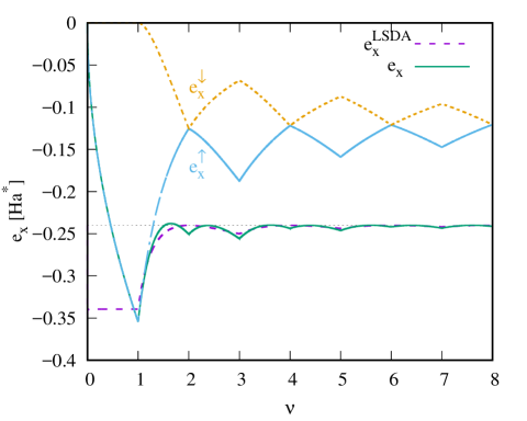
Figure 1: Exact-exchange energy per particle $e_{\text{x}}(r_{s},\nu)$ and its local spin density approximation $e_{\text{x}}^{\text{LSDA}}(r_{s},p(\nu))$ vs $\nu$, for $r_{s}=2.5$. The horizontal line at $-4\sqrt{2}/(3\pi r_{s})\simeq-\;0.24$ corresponds to the common $\nu\gg 1$ limit of $e_{\text{x}}(r_{s},\nu)$ and $e_{\text{x}}^{\text{LSDA}}(r_{s},p(\nu))$. The spin-discriminated contributions $e_{\text{x}}^{\uparrow}(r_{s},\nu)$ and $e_{\text{x}}^{\downarrow}(r_{s},\nu)$ are also displayed.

Fig. 1 shows the EE energy per particle vs $\nu$, for $r_{s}=2.5$  td . The LSDA result is also shown for comparison, using expression (30) and making the replacement $p\rightarrow p(\nu)=[\nu_{\uparrow}(\nu)-\nu_{\downarrow}(\nu)]/\nu$  note1 . The differences between both results increases when the magnetic field is increased (small $\nu$ limit). The exact-exchange energy displays derivative discontinuities at every integer filling factor $\nu$, while this kind of discontinuity is present in the LSDA energy only at odd integer values of $\nu$. In the LSDA the derivative of the exchange energy can be written as ${de_{\text{x}}^{\text{LSDA}}}/{d\nu}={de_{\text{x}}^{\text{LSDA}}}/{dp}\times{dp(\nu)}/{d\nu}$, and the discontinuities enter through ${dp}/{d\nu}$ that is discontinuous at every integer value of $\nu$. However, at even $\nu$ values ${de_{\text{x}}^{\text{LSDA}}}/{dp}=0$, the effect of ${dp(\nu)}/{d\nu}$ is lost, and the derivative is continuous at this points. The difference between the LSDA and EE is rooted in the fact that the LSDA is a zero magnetic-field approximation, reflected in the parity property that $e_{\text{x}}^{\text{LSDA}}(r_{s},p)=e_{\text{x}}^{\text{LSDA}}(r_{s},-p)$. This means that their expansion in the $p\rightarrow 0$ limit only involves even powers of $p$. This leads to the property ${de_{\text{x}}^{\text{LSDA}}}/{dp}=0$ for even $\nu$. On the other side, $e_{\text{x}}(r_{s},\nu)$ fully includes the effect of the magnetic field. Other interesting difference between these two approaches to the exchange energy is that the EE result presents local minima at every integer $\nu$ values, while the LSDA exchange energy has local minima only at odd $\nu$ and local maxima at even $\nu$. In the LSDA approach the exchange energy only depends (at constant density) on the polarization $p$, and the polarization presents local minima at even $\nu$ (loosing exchange energy) and local maxima at odd $\nu$’s (gaining exchange energy). The behavior of EE energy is however more complicated: besides $p$, it also depends of the occupation factor of the last occupied LL. The spin-discriminated EE energies are also displayed in Fig. 1. $e_{\text{x}}^{\uparrow}(r_{s},\nu)$ decreases when $[\nu]<\nu<[\nu]+1$, with $[\nu]=$ even, while it increases for $[\nu]<\nu<[\nu]+1$ when $[\nu]=$ odd. $e_{\text{x}}^{\downarrow}(r_{s},\nu)$ shows the opposite behavior. Both $e_{\text{x}}^{\uparrow}(r_{s},\nu)$ and $e_{\text{x}}^{\downarrow}(r_{s},\nu)$ have large derivative discontinuities of opposite signs at every integer $\nu$, that nearly compensates to give the much weaker, but still finite slope discontinuities of $e_{\text{x}}(r_{s},\nu)$.

Figure 2: Exact-exchange potential $v_{\text{x}}^{\sigma}(0)$ and its LSDA counterpart $v_{\text{x}}^{\sigma,{\text{L}SDA}}$ at $z=0$ vs $\nu$, for $r_{s}=2.5$. The horizontal line at $-2\sqrt{2}/(\pi r_{s})\simeq-\;0.36$ corresponds to the common $\nu\gg 1$ limit of $v_{\text{x}}^{\sigma}(0)$ and $v_{\text{x}}^{\sigma,\text{LSDA}}$.

We display in Fig. 2 the EE and LSDA exchange potentials for both spin components. $v_{\text{x}}^{\uparrow}(0)$ has sharp discontinuities at every even $\nu$, while $v_{\text{x}}^{\downarrow}(0)$ has the discontinuities located at odd values of $\nu$, excepting $\nu=1$. All these abrupt jumps are related to the filling of a new LL, as we will discuss below. On the other side, both components of the LSDA exchange potential are continuous, and only exhibits derivative discontinuities at every integer filling factor. $v_{\text{x}}^{\uparrow,\text{LSDA}}$ is constant for $0<\nu<1$, since for this strong field regime all electrons are fully spin-polarized in the ground LL, with $p=1$. The derivative discontinuities of $v_{\text{x}}^{\sigma,\text{LSDA}}$ are just a consequence of its dependence on $p(\nu)$, that also has a discontinuous derivative at every integer $\nu$. As has been already pointed out, the discontinuities in $v_{\text{x}}^{\sigma}(0)$ at integer $\nu$’s are due to the non-trivial behavior with magnetic field of the function $S_{2}^{\nu_{\sigma}}(0)$ in Eq. (14) or equivalently the function $\eta_{\text{x}}^{\sigma}$ in Eq. (25). Proceeding from this last equation, the abrupt jump in the EE exchange potential at every integer $\nu$ may be written exactly as

$$\Delta v_{\text{x}}^{\sigma}= \frac{-1}{r_{s}}\sqrt{\frac{2}{\nu}}\left[S_{2}^{[\nu_{\sigma}]^{+}}(0)-S_{2}^{[\nu_{\sigma}]^{-}}(0)\right]\;,$$

$$= \frac{-1}{r_{s}}\sqrt{\frac{2}{\nu}}\left[I_{2}([\nu_{\sigma}])-I_{2}([\nu_{\sigma}]-1)-I_{3}([\nu_{\sigma}]-1)\right]\;,$$

$$= \frac{1}{r_{s}}\sqrt{\frac{2}{\nu}}\int_{0}^{\infty}e^{-X}L_{[\nu_{\sigma}]-1}^{1}\left(X\right)$$

$$\times\left[L_{[\nu_{\sigma}]-1}^{0}\left(X\right)-L_{[\nu_{\sigma}]}^{0}\left(X\right)\right]\;dx\;,$$ (32)

with $X=x^{2}/2$. We have checked numerically that the last integral is finite and positive, for finite $[\nu_{\sigma}]$. On the other side, for $[\nu_{\sigma}]\gg 1$, the difference between the two generalized Laguerre polynomials inside the integral is increasingly small, and then the discontinuity in the EE also vanishes asymptotically in the low-field limit. Note however the quite different behavior of $e_{\text{x}}(r_{s},\nu)$ and of $v_{\text{x}}^{\sigma}(0)$ in the large $\nu$ limit: while for $\nu\sim 10$ $e_{\text{x}}(r_{s},\nu)$ and $e_{\text{x}}^{\text{LSDA}}(r_{s},p(\nu))$ are essentially indistinguishable on the drawing scale in Fig. 1, the difference between $v_{\text{x}}^{\sigma}(0)$ and $v_{\text{x}}^{\sigma,\text{LSDA}}$ are still clearly discernible in Fig. 2 for large $\nu$. This point will be discussed in more detail in the following section. It should be also emphasized that the jump given by $\Delta v_{\text{x}}^{\sigma}$ above applies also to the full exchange potential $v_{\text{x}}^{\sigma}(z)$, and not only to its strict-2D contribution $v_{\text{x}}^{\sigma}(0)$ discussed above. This issue is further discussed in the discussion surrounding Fig. 4.

III.2 Zero magnetic-field limit

From the previous results we can see that by decreasing the magnetic field (and then increasing $\nu$) the EE results somehow become similar to the LSDA results. Now we will shown that we can obtain the LSDA results analytically as a zero-field limit of our EE expressions. This can be considered as a critical test on the consistency of the present formalism. In the first place, the EE energy in expression (13) should reduce to expression (30). For proving that, we can write the EE energy per particle in the form,

$$e_{\text{x}}(r_{s},\nu)=-\frac{2\sqrt{2}}{3\pi r_{s}}\left\{[1+p(\nu)]^{3/2}\bar{S}_{1}^{\nu_{\uparrow}}+[1-p(\nu)]^{3/2}\bar{S}_{1}^{\nu_{\downarrow}}\right\}\;,$$ (33)

with $\bar{S}_{1}^{\nu_{\sigma}}=(3\pi/8\sqrt{2})S_{1}^{\nu_{\sigma}}(0)/\nu_{\sigma}^{3/2}$. This re-writing is motivated by the fact that now the difference between the EE and LSDA exchange energies is just related to how far are the factors $\bar{S}_{1}^{\nu_{\sigma}}$ from unity. Using that (see Appendix A, Eq. (A.8))

$$\lim_{\nu_{\sigma}\rightarrow\infty}\bar{S}_{1}^{\nu_{\sigma}}\rightarrow 1\;,$$ (34)

we have

$$\lim_{\nu\rightarrow\infty}e_{\text{x}}(r_{s},\nu)=e_{\text{x}}^{{\text{LSDA}}}(r_{s},p)\;,$$ (35)

where we have used that $p(\nu)=[\nu_{\uparrow}(\nu)-\nu_{\downarrow}(\nu)]/\nu$. This last result is the well-know exchange energy of the strict-2D electron gas at zero magnetic-field presented above.

On the other hand the limit $\nu\gg 1$ of the EE potential at $z=0$, that is, the potential at the electron gas should coincide also with the respective strict-2D zero-field LSDA result. For the EE potential we can work in a similar way as with the energy, doing a re-writing of Eq. (25)

$$v_{\text{x}}^{\sigma}(z=0)=-\frac{2\sqrt{2}}{\pi r_{s}}\left[1\pm p(\nu)\right]^{1/2}\bar{S}_{2}^{\nu_{\sigma}}\;,$$ (36)

with $\bar{S}_{2}^{\nu_{\sigma}}=(\pi/2\sqrt{2})S_{2}^{\nu_{\sigma}}(0)/\nu_{\sigma}^{1/2}$. Using now that (see Appendix A, Eq. (A.9))

$$\lim_{\nu_{\sigma}\rightarrow\infty}\bar{S}_{2}^{\nu_{\sigma}}\rightarrow 1 \;,$$ (37)

we obtain

$$\lim_{\nu\rightarrow\infty}v_{\text{x}}^{\sigma}(z=0)=v_{\text{x}}^{\sigma,{\text{LSDA}}}\;,$$ (38)

the same expression as in the zero-field case. These two quantities $\bar{S}_{1}^{\nu_{\sigma}}$ and $\bar{S}_{2}^{\nu_{\sigma}}$ may be considered as a sort of finite-$\nu$ “correction” factors, whose inclusion brings the LSDA results towards the EE expressions.

In Fig. 3 we shown how these two “correction” factors approach the LSDA limit as $\nu$ increases, for the spin-up case. While it is seen there that $\bar{S}_{1}^{\nu_{\uparrow}}$ approach the large $\nu$ limit of Eq. (34) quite rapidly, the approach of $\bar{S}_{2}^{\nu_{\uparrow}}$ to the LSDA limit is much slower, that explains the persistence of sizeable discontinuities in $v_{\text{x}}^{\uparrow}(0)$ in Fig. 2, even for large values of $\nu$.

The abrupt jump expression for $\Delta v_{\text{x}}^{\sigma}$ may be also analyzed by using the asymptotic expansions for $I_{2}(n)$ and $I_{3}(n)$ given in the Appendix. Since $I_{2}([\nu_{\sigma}])\sim([\nu_{\sigma}])^{1/2}$ and $I_{3}([\nu_{\sigma}])\sim\ln([\nu_{\sigma}])/([\nu_{\sigma}])^{1/2}$ for large $\nu_{\sigma}$, in the same low-field limit $\Delta v_{\text{x}}^{\sigma}$ vanishes asymptotically as $\ln([\nu_{\sigma}])/[\nu_{\sigma}]$. This is consistent with the fact that the LSDA exchange potential, that corresponds to the $\nu_{\sigma}\rightarrow\infty$ limit has no discontinuities at integer filling factors.

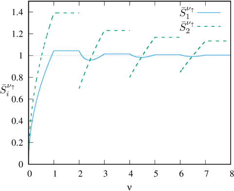
Figure 3: $\bar{S}_{1}^{\nu_{\uparrow}}$ and $\bar{S}_{2}^{\nu_{\uparrow}}$ as function of the filling factor $\nu$. The LSDA limit at $\nu\gg 1$ is represented by the horizontal line at unity, and it is seen as they approach this limit in quite different ways. $\bar{S}_{2}^{\nu_{\uparrow}}$ has an abrupt jump at every even $\nu$.

It is important to remark the importance of the inclusion of $\eta_{\text{x}}^{\sigma}$ term, which comes from the implicit derivative of the exchange energy with respect to the density. This term is the origin of derivative discontinuity and without it we cannot obtain the correct zero magnetic-field limit.

III.3 On the z-dependence of $v_{\text{x}}^{\sigma}(z)$

Up to this point we have only considered the EE potential at the electron gas coordinate $z=0$. But as we have already discussed, the present procedure has the advantage that it provides quite naturally also its $z$-dependence, as follows.

Fig. 4 displays the spin-up EE potential as defined in Eq. (14), as a function of $z$ and for several values of $\nu$, either approaching an even integer filling factor from above ($\nu^{+}$), or from below ($\nu^{-}$). Several interesting features of Fig. 4 are worth of be commented: i) it gives a more complete perspective about how the EE potential discontinuity present at every integer $\nu$ at $z=0$ and displayed in Fig. 2 evolves with the distance $z$; ii) while the EE potentials corresponding to $\nu^{+}$ approach the zero-field limit from above for increasing values of $\nu$, the ones corresponding to $\nu^{-}$ approach the same limit from below; and iii) in the asymptotic limit $|z|/l_{B}\gg 1$, the EE potential approach a finite non-negative value, that depends on the density and the magnetic field.

This last point can be further elaborated analytically: the large $z$-limit of $v_{\text{x}}^{\sigma}(z)$ is given by the large $z$-limit of $S_{1}^{\nu_{\sigma}}(|z|)$ in Eq. (14). Now, according Eq. (11), what matters for this limit is how the functions $I_{n}^{m}(t)$ behave for large values of their argument. Inspection of Eq. (4) reveals that for $|z-z^{\prime}|/l_{B}\gg 1$, only the limit of the integrand for small values of $x$ contributes to the integral. Considering that $L_{n_{<}}^{n_{>}-n_{<}}(0)=n_{>}!/n_{<}!(n_{>}-n_{<})!$, we have then

$$I_{n}^{m}\left(\frac{|z|}{l_{B}}\gg 1\right) \rightarrow \frac{n_{>}!}{n_{<}![(n_{>}-n_{<})!]^{2}}$$

$$\times \int_{0}^{\infty}\left(\frac{x^{2}}{2}\right)^{n_{>}-n_{<}}e^{-x|z|/l_{B}}dx$$

$$=\frac{n_{>}![2(n_{>}-n_{<})]!}{n_{<}![(n_{>}-n_{<})!]^{2}} \times \frac{1}{2^{(n_{>}-n_{<})}}\left(\frac{l_{B}}{|z|}\right)^{1+2(n_{>}-n_{<})}\;.$$

From this last expression is clear that the leading contribution to $I_{n}^{m}(|z|/l_{B}\gg 1)$ corresponds to $n_{>}=n_{<}$, and then to $n=m$: $I_{n}^{m}(|z|/l_{B}\gg 1)\rightarrow I_{n}^{n}(|z|/l_{B}\gg 1)=l_{B}/|z|$. And since $\sum_{n}^{[\nu_{\sigma}]-1}I_{n}^{n}(|z|/l_{B}\gg 1)=[\nu_{\sigma}]$ we obtain

$$v_{\text{x}}^{\sigma}(|z|/l_{B}\gg 1)\rightarrow C(r_{s},\nu)-\frac{[\nu_{\sigma}]+p_{\sigma}^{2}}{z\nu_{\sigma}}\;,$$ (40)

where

$$C(r_{s},\nu)=\frac{1}{r_{s}\nu_{\sigma}}\sqrt{\frac{2}{\nu}}\left[S_{1}^{\nu_{\sigma}}(0)-\nu_{\sigma}S_{2}^{\nu_{\sigma}}(0)\right]\;.$$ (41)

We have checked numerically that the term $C(r_{s},\nu)$ is always non-negative; besides, it is equal to zero only when $0<\nu_{\sigma}<1$ constant . Interestingly we obtain the universal $1/z$ asymptotic behavior RHP15 only in the limits of $p_{\sigma}\rightarrow(0,1)$ nuinteger . In Fig. 4 we compare this asymptotic behavior with the EE potential for $\nu=2^{+}$, and it is seen how the asymptotic limit is reached for $|z|/l_{B}\sim 10$.

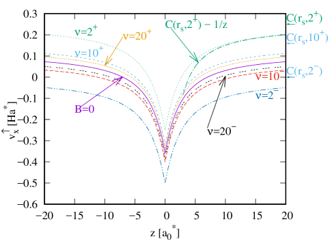
Figure 4: Exact-exchange potential vs $z$ for different filling factors. The EE potential for the spin-unpolarized 2D electron gas at zero magnetic field is also shown for comparison. The result for $\nu=2^{+}$ is compared with the expected asymptotic behavior for large $z$. The asymptotic limits for same of the potentials are given on the right vertical axis, and marked with arrows.

For the sake of completeness, we provide here also the spin-polarized EE potential at zero-magnetic field, which is given by HPR97

$$v_{\text{x}}^{\sigma,B=0}(z)= -\frac{1}{|z|}\left(1+\frac{L_{1}(2|z|^{*})-I_{1}(2|z|^{*})}{|z|^{*}}\right)$$

$$+\frac{2\sqrt{2}}{3\pi r_{s}}\sqrt{1\pm p}\;,$$ (42)

with $L_{1}(x)$ and $I_{1}(x)$ being the Struve and the modified Bessel functions, respectively, and $|z|^{*}=\sqrt{2(1\pm p)}|z|/r_{s}$. This expression has been obtained from the quasi-2D EE integro-differential equation at zero magnetic field, after imposing the same one-subband constraint and strict-2D limit as in the present contribution. Its derivation will be given elsewhere. While in principle it is feasible to obtain it by taking the zero-field limit of Eq. (14), the lack of the simplifying identities in Eqs. (20), (21), and (22) makes all the calculations much more involved. Using that the limit of $1+(L_{1}(2x)-I_{1}(2x))/x$ for $x\rightarrow 0$ is given by $8x/3\pi$, by evaluating the zero-field EE potential at $z=0$ one obtains

$$v_{\text{x}}^{\sigma,B=0}(z=0)=-\frac{2\sqrt{2}}{\pi r_{s}}\sqrt{1\pm p}\;,$$ (43)

that coincides with the zero-field limit of Eq. (38), as it should be. It is important to note that this internal consistency is only possible if the constant term $\frac{2\sqrt{2}}{3\pi r_{s}}\sqrt{1\pm p}$ is present in Eq. (42).

The $z$-dependence of the EE potential can be useful for the study of coupled 2D electron gases like bilayers HMD00 and trilayers HM96 ; MP16 ; WMGRBP09 ; MPB16 , in which this dependence appears as an inter-layer exchange term.

IV Conclusions

Starting from a general exact-exchange quasi-2D formalism describing an electron gas confined in a semiconductor quantum well in the regime of the integer quantum Hall effect, we have obtained its strict-2D projection. The corresponding strict-2D calculations are much simpler than the ones associated with the quasi-2D case, since in the latter situation the self-consistent Kohn-Sham orbitals describing the subband physics must be obtained numerically. Instead, in our strict-2D evaluation, these Kohn-Sham orbitals are replaced by Dirac delta-functions, that constraints the electron dynamics to a single plane. As the filling of the emerging Landau levels proceeds, two main features results: i) the EE energy minimizes with a discontinuous derivative at every integer filling factor $\nu$; and ii) the EE potential display sharp discontinuities at every integer $\nu$. On the other side, the standard strict-2D LSDA displays derivative discontinuities in the exchange energy only at odd filling factors, and has no discontinuities in the corresponding exchange potential. It should be emphasized that these important differences between LSDA and EE at finite magnetic fields are present even when both are based in the same density, that remains homogeneous at finite magnetic field. More to the point, the differences are due to the fact that the functional form of the EE energy fully includes the effect of the magnetic field through the Landau orbitals, while the LSDA is a zero-field approximation.

The present work suggest, however, in a very natural way how to go beyond the strict-2D LSDA as applied in the strong magnetic field regime of inhomogeneous two-dimensional electron systems: replace $v_{\text{x}}^{\sigma,{\text{LSDA}}}$ of Eq. (31) by $v_{x}^{\sigma}(0)$ of Eq. (36). In the standard LSDA, the zero-field expression for the homogeneous 2D electron gas, $v_{\text{x}}^{\sigma,{\text{LSDA}}}$ is applied to the finite magnetic field and inhomogeneous case by doing the local-density-approximation, that amounts to the replacements $r_{s}\rightarrow r_{s}(\bm{\rho})=1/\sqrt{\pi n(\bm{\rho})}$, and $p\rightarrow p(\bm{\rho})=(n_{\uparrow}(\bm{\rho})-n_{\downarrow}(\bm{\rho}))/n(\bm{\rho})$. Under these assumptions, $v_{\text{x}}^{\sigma,{\text{LSDA}}}$ becomes a position-dependent potential $v_{\text{x}}^{\sigma,{\text{LSDA}}}\rightarrow v_{\text{x}}^{\sigma,{\text{LSDA}}}(\bm{\rho})$. We suggest here that a more founded procedure will be to do the same local-density-approximation, but for our EE potential: $v_{\text{x}}^{\sigma}(0)\rightarrow v_{\text{x}}^{\sigma}(\bm{\rho},0)$. The crucial difference between $v_{\text{x}}^{\sigma,{\text{LSDA}}}(\bm{\rho})$ and $v_{\text{x}}^{\sigma}(\bm{\rho},0)$ is that while in the former the effect of the magnetic field enters indirectly through the field-induced changes in the spin-polarization, in $v_{\text{x}}^{\sigma}(\bm{\rho},0)$ the impact of the field is direct, since the functional form of the EE already fully contains the magnetic field. In other words, while $v_{\text{x}}^{\sigma}(\bm{\rho},0)$ is exact in the case of the uniform 2D gas at arbitrary magnetic field, $v_{\text{x}}^{\sigma,{\text{LSDA}}}(\bm{\rho})$ only is exact for the case of the homogeneous 2D gas at zero magnetic-field.

V Acknowledgements

DM and CRP acknowledge the financial support of ANPCyT under grant PICT 2016-1087, and CONICET under grant PIP 2014-2016 00402.

Appendix A Zero field limits

The analysis of the zero magnetic-field limit amounts to study the large $n$-limit of the functions $I_{1}(n)$, $I_{2}(n)$, and $I_{3}(n)$, defined in Eqs. (20), (21), and (22), respectively.

Starting with $I_{1}(n)$, we have that in the large-$n$ limit

$${}_{3}F_{2}\left(-n,\frac{1}{2},-\frac{1}{2};2,-n-\frac{1}{2};1\right)=\sum_{k=0}^{\infty}\frac{(-n)_{k}(\frac{1}{2})_{k}(-\frac{1}{2})_{k}}{k!(2)_{k}(-n-\frac{1}{2})_{k}}\;,$$

$$\simeq\sum_{k=0}^{\infty}\frac{(\frac{1}{2})_{k}(-\frac{1}{2})_{k}}{(2)_{k}}\frac{1}{k!}={}_{2}F_{1}\left(\frac{1}{2},-\frac{1}{2};2;1\right)\;.$$

Using now the relation AS

$${}_{2}F_{1}\left(a,b;c;1\right)=\frac{\Gamma(c)\Gamma(c-a-b)}{\Gamma(c-a)\Gamma(c-b)}\;,$$ (A.2)

we obtain that ${}_{2}F_{1}\left(\frac{1}{2},-\frac{1}{2};2;1\right)=\frac{8}{3\pi}$. Collecting all results so far,

$$I_{1}(n+1)\simeq\frac{8}{3\sqrt{2\pi}}\frac{(2)_{n}(3/2)_{n}}{(n!)^{2}}\;.$$ (A.3)

In the last step, since the Pochhammer’s symbols admit the asymptotic expansion

$$(a)_{n}\simeq\frac{\sqrt{2\pi}}{\Gamma(a)}e^{-n}n^{a+n-1/2}\left[1+\mathcal{O}(1/n)\right]\;,$$ (A.4)

and using the Stirling approximation $n!\simeq\sqrt{2\pi}n^{n+1/2}e^{-n}$, we obtain that

$$I_{1}(n+1)\simeq\frac{8\sqrt{2}}{3\pi}n^{3/2}+\mathcal{O}\left({n^{1/2}}\right)\;.$$ (A.5)

Regarding the large-$n$ limit of $I_{2}(n)$, we are now concerned with the asymptotic limit of

$${}_{3}F_{2}\left(-n,\frac{1}{2},-\frac{1}{2};1,\frac{1}{2}-n;1\right)=\sum_{k=0}^{\infty}\frac{(-n)_{k}(\frac{1}{2})_{k}(-\frac{1}{2})_{k}}{k!(1)_{k}(\frac{1}{2}-n)_{k}}\;,$$

$$\simeq\sum_{k=0}^{\infty}\frac{(\frac{1}{2})_{k}(-\frac{1}{2})_{k}}{(1)_{k}}\frac{1}{k!}={}_{2}F_{1}\left(\frac{1}{2},-\frac{1}{2};1;1\right)=\frac{2}{\pi}\;.$$

In the last step we have used Eq. (A.2) again. Returning to Eq. (21),

$$I_{2}(n)\simeq\sqrt{\frac{2}{\pi}}\frac{(1)_{n}(3/2)_{n-1}}{n!(n-1)!}\simeq\frac{2\sqrt{2}}{\pi}n^{1/2}+\mathcal{O}\left(\frac{1}{n^{1/2}}\right)\;.$$ (A.7)

Regarding the large-$n$ limit of $I_{3}(n)$, we have numerical evidence that $I_{3}(n)\sim\ln(n)/n^{1/2}$ for $n\gg 1$. The scalings $I_{1}(n)\sim n^{3/2}$ and $I_{2}(n)\sim n^{1/2}$ are easy of understand from the corresponding definitions in Eq. (18): for a given scaling of $I_{3}(n)$, $I_{2}(n)$ has about $n$ contributions more, while $I_{1}(n)$ has a double sum with about $n^{2}$ terms. This is understable also from a physical point of view: the contribution to the EE energy and potential of the last fractionally occupied LL should be negligible when the number of fully occupied LL becomes very large.

Putting all results together,

$$\lim_{\nu_{\sigma}\rightarrow\infty}\bar{S}_{1}^{\nu_{\sigma}}= \frac{3\pi}{8\sqrt{2}}\lim_{\nu_{\sigma}\rightarrow\infty}\frac{I_{1}([\nu_{\sigma}])+2p_{\sigma}I_{2}([\nu_{\sigma}])+p_{\sigma}^{2}I_{3}([\nu_{\sigma}])}{\nu_{\sigma}^{3/2}}$$

$$\rightarrow 1\;.$$ (A.8)

In a similar way we can show that

$$\lim_{\nu_{\sigma}\rightarrow\infty}\bar{S}_{2}^{\nu_{\sigma}}= \frac{\pi}{2\sqrt{2}}\lim_{\nu_{\sigma}\rightarrow\infty}\frac{(I_{2}([\nu_{\sigma}])+p_{\sigma}I_{3}([\nu_{\sigma}])}{\nu_{\sigma}^{1/2}}$$

$$\rightarrow 1.$$ (A.9)

In principle, from the corrections to the leading term in Eqs. (A.5) and (A.7) is feasible to obtain the corresponding corrections to the leading (LSDA) limits for $e_{\text{x}}(r_{s},\nu)$ and $v_{\text{x}}^{\sigma}(z)$, as given by Eqs. (35) and (38), respectively. Since the final results are somehow involved, they will be given elsewhere.

References

• (1) J. Weis and K. von Klitzing, Philos. Trans. R.Soc. A 369, 3954 (2011).
• (2) S. das Sarma and A. Pinczuk, in Perspectives in Quantum Hall Effects (Wiley,New York,1997).
• (3) G. F. Giuliani and G. Vignale in Quantum Theory of the Electron Liquid, Cambridge University Press, Cambridge, (2005).
• (4) D. Miravet, G. J. Ferreira and C. R. Proetto, Europhys. Lett. 119, 57001 (2017).
• (5) R. G. Parr and W. Yang, in Density Functional Theory of Atoms and Molecules (Oxford University Press, New York, 1989); R. M. Dreizler and E. K. U. Gross, in Density Functional Theory (Springer, Berlin, 2000).
• (6) T. Grabo, T. Kreibich, S. Kurth, and E. K. U. Gross in Strong Coulomb Interactions in Electronic Structure Calculations: Beyond the Local Density Approximation, edited by V. I. Anisimov (Gordon and Breach, Amsterdam, 2000).
• (7) S. Pittalis, S. Kurth, N. Helbig, and E. K. U. Gross, Phys. Rev. A 74, 065511 (2006); S. Sharma, J. K. Dewhurst, C. Ambrosch-Draxl, S. Kurth, N. Helbig, S. Pittalis, S. Shallcross, L. Nordström, and E. K. U. Gross, Phys. Rev. Lett. 98, 196405 (2007); N. Helbig, S. Kurth, S. Pittalis, E. Räsänen, and E. K. U. Gross, Phys. Rev. B 77, 245106-1 (2008).
• (8) S. Becker, C. Karrasch, T. Mashoff, M. Pratzer, M. Liebmann, V. Meden, and M. Morgenstern, Phys. Rev. Lett. 106, 156805 (2011).
• (9) G. Bastard, in Wave mechanics applied to Semiconductor Heterostructures (Les Editions de Physique, Les Ulis, 1988).
• (10) E. Räsänen, H. Saarikoski, A. Harju, M. Ciorga, and A. S. Sacharjda, Phys. Rev. B 77, 041302(R) (2008).; M. C. Rogge, E. Räsänen, and R. J. Haug, Phys. Rev. Lett. 105 046802 (2010); H. Atci, U. Erkarslan, A. Siddiki, and E. Räsänen, J. Phys.: Condens. Matter 25 155604 (2013); H. Atci and A. Siddiki, Phys. Rev. B 95, 045132 (2017).
• (11) M. Ferconi and G. Vignale, Phys. Rev. B 52, 16357 (1995); O. Heinonen, M. I. Lubin, and M. D. Johnson, Phys. Rev. Lett. 75, 4110 (1995); J. Zhao, M. Thakurathi, M. Jain, D. Sen, and J. K. Jain, Phys. Rev. Lett. 118, 196802 (2017).
• (12) The dimensionless $\nu$ is defined as $\nu=N/N_{\phi}$, with $N$ being the total number of electrons, and $N_{\phi}=AB/\Phi_{0}$ the Landau level degeneracy. Here $A$ is the area of the sample in the $x-y$ plane ($A^{*}$ in $(a_{0}^{*})^{2}$ units), $B$ is the magnetic field strength, and $\Phi_{0}=ch/e$ is the magnetic flux number. Note that $\nu$ may be written as the ratio between two quantities with dimensions of 2D densities: $\nu=(N/A)/(B/\Phi_{0})$.
• (13) C. B. Hanna and A. H. Macdonald, Phys. Rev. B 53, 15981 (1996).
• (14) For material parameters corresponding to GaAs as well-acting semiconductor, $Ha^{*}\simeq 11.04$ meV, and $a_{0}^{*}\simeq 101.5\;\AA$.
• (15) D. Miravet and C. R. Proetto, Phys. Rev. B 94, 085304 (2016).
• (16) A. P. Prudnikov, Yu. A. Brychkov, and O. I. Marichev, in Integrals and Series, Volume 2, Special Functions (Gordon and Breach,New York,1986). See Eq. 2.19.14.15 in page 478.
• (17) M. Abramowitz and I. A. Stegun in Handbook of Mathematical Functions (Dover,New York,1972).
• (18) For material parameters corresponding to GaAs as well-acting semiconductor, $r_{s}=2.5$ corresponds to a 2D density equal to $4.9\times 10^{10}$/cm2, which is a typical density for the 2D semiconductor systems addressed in this work.
• (19) Note that formally this replacement may be motivated by using the relation $n_{\sigma}=\nu_{\sigma}N_{\phi}$.
• (20) As stated below Eq. (12), for $[\nu_{\sigma}]=0$, $S_{1}^{\nu_{\sigma}}(0)=\nu_{\sigma}^{2}I_{0}^{0}(0)$, and $S_{2}^{\nu_{\sigma}}(0)=\nu_{\sigma}I_{0}^{0}(0)$, leading to $C(r_{s},0<\nu_{\sigma}<1)=0$.
• (21) S. Rigamonti,C. M. Horowitz and C. R. Proetto, Phys. Rev. B 92, 235145 (2015).
• (22) Note that at zero-temperature the EE potential is non-defined for integer $\nu$, because of the discontinuities.
• (23) C. Horowitz, C. R. Proetto, and S. Rigamonti, Phys. Rev. Lett. 97, 026806 (2006); S. Rigamonti and C. R. Proetto, Phys. Rev. B 73, 235319 (2006).
• (24) T. Jungwirth and A. H. MacDonald, Phys. Rev. B 63, 035305 (2000).
• (25) S. Wiedmann, N. C. Mamani, G. M. Gusev, O. E. Raichev, A. K. Bakarov, and J. C. Portal, Phys. Rev. B 80, 245306 (2009).
• (26) D. Miravet, C. R. Proetto and P. G. Bolcatto, Phys. Rev. B 93, 085305 (2016).