Classical and quantum spin dynamics of the honeycomb $\Gamma$ model

Abstract

Quantum to classical crossover is a fundamental question in dynamics of quantum many-body systems. In frustrated magnets, for example, it is highly non-trivial to describe the crossover from the classical spin liquid with a macroscopically-degenerate ground-state manifold, to the quantum spin liquid phase with fractionalized excitations. This is an important issue as we often encounter the demand for a sharp distinction between the classical and quantum spin liquid behaviors in real materials. Here we take the example of the classical spin liquid in a frustrated magnet with novel bond-dependent interactions to investigate the classical dynamics, and critically compare it with quantum dynamics in the same system. In particular, we focus on signatures in the dynamical spin structure factor. Combining Landau-Lifshitz dynamics simulations and the analytical Martin-Siggia-Rose (MSR) approach, we show that the low energy spectra are described by relaxational dynamics and highly constrained by the zero mode structure of the underlying degenerate classical manifold. Further, the higher energy spectra can be explained by precessional dynamics. Surprisingly, many of these features can also be seen in the dynamical structure factor in the quantum model studied by finite-temperature exact diagonalization. We discuss the implications of these results, and their connection to recent experiments on frustrated magnets with strong spin-orbit coupling.

I Introduction

The crossover between classical and quantum regimes in frustrated magnets has been an important theoretical question in the last few decades. This issue is particularly important in understanding the nature of the quantum spin liquid phases which may arise at low temperature due to extreme quantum fluctuations. In the classical regime, there may exist a window of temperatures below the Curie-Weiss scale, where the correlated spin moments are thermally fluctuating within the degenerate manifold of classical ground states. This is the cooperative paramagnetic state, or the so-called classical spin liquid. In the quantum regime, it is clearly not possible to maintain such a state down to zero temperature as the quantum ground state should be unique (up to a topological degeneracy in the case of quantum spin liquids). An important question is how much information about the degenerate manifold of classical ground states is encoded in the emergent quantum spin liquid at zero and low temperatures. Such a question may be especially relevant for two dimensional spin liquid phases which show no finite temperature phase transition, but only crossovers.

One natural place to look for the clue for this question is the dynamical spin correlation or the dynamical spin structure factor. A recent work on the Kitaev modelKitaev (2006) in two dimensions investigates the dynamical spin correlations of the classical Kitaev model via Landau-Lifshitz (LL) dynamics Samarakoon et al. (2017). The resulting dynamical structure factor was compared with that of the quantum modelKnolle et al. (2014, 2015); Baskaran et al. (2007), which is exactly solvable and supports a quantum spin liquid ground state with gapless Majorana fermion excitations. There exist two crossover temperatures, $T_{v}$ and $T_{Q}$, in the Kitaev model on the honeycomb lattice, as seen in the specific heat.Nasu et al. (2015) At $T<T_{v}$, the vison or flux gap is larger than the temperature scale so that the system is essentially characterized by the zero temperature ground state. When $T_{v}<T<T_{Q}$, the flux degree of freedom is thermally disordered, but the Majorana fermions are still well defined. For $T>T_{Q}$, the system crosses over to the classical regime. It was found that the dynamical spin correlations in the quantum model at $T>T_{v}$ are remarkably similar to those of the cooperative paramagnetic regime of the classical model at finite temperature. Moreover, the dynamical structure factor of the quantum model knows about the zero mode structure of the classically degenerate manifold even when $T_{v}<T<T_{Q}$. This suggests that all the classically degenerate spin states are participating in the quantum fluctuations down to $T\sim T_{v}$, which eventually lead to the emergence of the quantum spin liquid phase at low temperature $T<T_{v}$.

In principle, it is not necessary that the full degenerate manifold of the classical states is involved in the formation of the quantum spin liquid at low temperature, since thermal entropy or zero-point quantum fluctuations may select a subset of the full degenerate manifold at some intermediate temperature. On the other hand, when the full degenerate manifold is participating in quantum fluctuations at low temperature, as the case of the Kitaev model for $T_{v}<T<T_{Q}$, and if the spin correlations remain short-ranged, it is highly suggestive that the zero temperature ground state would indeed be a quantum spin liquid. An alternative choice for the zero temperature ground state could be a magnetically ordered state or a quantum critical point, which would show the development of long-range dynamical spin fluctuations. In the case of the Kitaev model, we already know that this is not the case, and that the zero temperature ground state is a quantum spin liquid. One may, however, be able to use this lesson to infer the possible presence of a quantum spin liquid in models which are not exactly solvable.

In the current work, we investigate the dynamical spin correlations in the classical and quantum $\Gamma$ modelRau et al. (2014) (defined below) on the honeycomb lattice, which is known to possess macroscopically degenerate manifold of classical ground statesRousochatzakis and Perkins (2017), while the quantum model is not exactly solvable. This model represents the bond-dependent anisotropic and symmetric spin interactions on the honeycomb lattice:

$${\cal H}=\;\;\mathrm{\Gamma}\sum_{\alpha\neq\beta\neq\gamma}{\sum_{\left\langle{\bm{r}},{\bm{r}}^{\prime}\right\rangle\ \in\ \gamma}{\mathrm{(}S^{\beta}_{\bm{r}}S^{\alpha}_{{\bm{r}}^{\prime}}\mathrm{+}S^{\alpha}_{\bm{r}}S^{\beta}_{{\bm{r}}^{\prime}}\mathrm{)}}},$$ (1)

where $S^{\alpha}_{\bm{r}}$ are spin operators at sites $\bm{r}$ of a honeycomb lattice, and $\alpha,\beta,\gamma=x,y,z$. Such interactions (as well as the Kitaev interaction mentioned above) arise in strongly spin-orbit coupled Mott insulators such as Li₂IrO₃ and $\alpha$-RuCl₃, where Ir⁴⁺ or Ru³⁺ ions form effective $J=1/2$ local moments. Currently, the relative importance of the Kitaev and $\Gamma$ interactions is an important issue in theoretical and experimental investigations of this class of Kitaev-like materialsJackeli and Khaliullin (2009); Witczak-Krempa et al. (2014); Rau et al. (2014); Plumb et al. (2014); Sears et al. (2015); Johnson et al. (2015); Rau et al. (2016); Winter et al. (2016, 2017a); Trebst (2017); Sears et al. (2017); Do et al. (2017); Hentrich et al. (2018); Wolter et al. (2017); Winter et al. (2017b, 2018). For instance, the dominance of one of these interactions or the cooperation of these two interactions may lead to possible emergence of quantum spin liquid in these materials, especially in the presence of external pressure or magnetic field.

We first use the Landau-Lifshitz dynamics to compute the dynamical structure factor in the classical model at finite temperature. It is shown that the zero mode structure of the degenerate manifold of classical ground states is reflected in the low frequency part of the dynamical spin fluctuation spectra. For example, in the case of the antiferro-sign of the $\Gamma>0$ interaction, the structure factor at low frequencies is suppressed at the $\bm{\Gamma}$ and $\bm{X}$ points of the Brillouin zone, which we explain using the constraints on the classical spin states which belong to the degenerate manifold. Next, we employ the Martin-Siggia-Rose (MSR) formulation of Langevin dynamics to further understand the nature of the dynamical spin correlations. These two different methods lead to essentially the same dynamical spin correlations, leading to the conclusion that the system itself may be acting as an effective thermal bath. Furthermore, it is shown that the low frequency response is relaxational and reflects the zero mode structure, while the higher frequency response is mostly precessional, and some characteristic precessional modes exist at finite frequencies. The evolution of dynamical spin correlations is also investigated as a function of temperature for the comparison with the quantum model.

The dynamical spin structure factor in the quantum $\Gamma$ model is studied by exact diagonalization via the shifted Krylov subspace method, which is combined with typical quantum state approach at finite temperature. In previous studiesCatuneanu et al. (2018), it was shown that there exist two crossover temperatures, $T_{1}\sim 0.03\Gamma$ and $T_{2}\sim 0.4\Gamma$, in the specific heat, similar to the case of the Kitaev model. $T_{2}$ marks the crossover from the high temperature classical regime to the quantum regime. We find that the dynamical spin correlations at low frequencies in the quantum model show distinct signatures of the zero mode structure of the degenerate manifold of classical ground states even when $T_{1}<T<T_{2}$, which gradually crosses over to the low temperature extreme quantum limit for $T<T_{1}$. This behavior is reminiscent of the dynamical spin correlations in the Kitaev model, where correlations as a function of temperature are remarkably similar to the classical result. This means that the short-range spin fluctuations from the degenerate manifold persist even in the quantum regime of $T_{1}<T<T_{2}$. On the other hand, the dynamical spin correlations at zero temperature, while they remain short-ranged, show features that are not present in the classical model. In the case of $\Gamma$ model, we currently do not know what the quantum ground state is. One possibility is that below a certain temperature a symmetry is broken due to order by quantum disorderRousochatzakis and Perkins (2017). Interestingly, however, recent DMRG and exact diagonalization studies suggest possible presence of a quantum spin liquid ground state in the $\Gamma$ modelGohlke et al. (2018). Since we do not have an analytical understanding of the underlying quasiparticles in the $\Gamma$ model, we cannot make a more precise connection to underlying quantum degrees of freedom, which was possible in the case of the Kitaev model. Nonetheless, the phenomenological similarity to the classical-quantum correspondence in the Kitaev model is striking. We may speculate that the entire degenerate manifold of classical states would participate in quantum fluctuations that lead to the formation of the quantum ground state at zero temperature, such as a quantum spin liquid phase. Our findings will help understanding this outstanding issue and possible connection to experiments on Kitaev-like materials.

The rest of the paper is organized as follows. In section II, we present numerical results obtained from the LL dynamics of the classical model. Section III describes how qualitatively similar results can be obtained analytically within an MSR formalism. The dynamic correlations of the corresponding quantum model are given in section IV. We conclude with a discussion of our main findings in light of recent experiments in section V, while details of our calculations are relegated to the appendices.

II Landau-Lifshitz dynamics

We study the dynamical spin correlations of the $\Gamma$ model, Eq. (1), whereby the spin operators are replaced by classical vectors in the Heisenberg equation of motion. The resulting Landau-Lifshitz (LL) equation of motion is

$$\frac{d{\bm{S}}_{\bm{r}}}{dt}\mathrm{=}{\bm{S}}_{\bm{r}}\mathrm{\times}{\bm{B}}_{\bm{r}},$$ (2)

where ${\bm{B}}_{\bm{r}}$ is the molecular field acting on the spin ${\bm{S}}_{\bm{r}}$. This LL equation can be solved numerically by applying a fourth order Runge-Kutta algorithm with adaptive step size. The average over configurations at a given temperature $T$ is obtained from the Metropolis Monte Carlo sampling method. We note that a closed LL dynamics is more appropriate than Langevin dynamics when the experiment is much faster than the spin-lattice relaxation, which is the typical case in inelastic neutron-scattering experiments. The simulations are performed on a finite lattice of 30$\times$30 unit-cells (1800 spins) with periodic boundary conditions.

Fig. 1 shows the trace of the dynamical spin structure factor, $S\left({\bm{Q}},\omega\right)=\ \sum_{\alpha}{S^{\alpha\alpha}\left({\bm{Q}},\omega\right)}$, obtained for the antiferromagnetic (AFM) (${\mathrm{\Gamma}}>0$) and ferromagnetic (FM) ($\mathrm{\Gamma}<0$) versions of the $\Gamma$-model. As expected for a liquid state, $S\left({\bm{Q}},\omega\right)$ exhibits a continuum of low and high-frequency modes. The low-frequency (zero) modes arise from the very slow dynamics through different classical ground states. The number of zero modes is macroscopic because of the extensive residual entropy of the ground state manifold. This dynamics is expected to be relaxational because the average of the local field over a period $2\pi/\omega$ is equal to zero. In contrast, the high-frequency modes correspond to the much faster spin precession around the local fields produced by a given ground state configuration. Accordingly, the average of the local fields ${\bm{B}}_{\bm{r}}$ over a period $2\pi/\omega$ remains finite.

Both, the low and high-frequency modes, contain relevant information about the liquid state. The momentum distribution of the zero-energy modes is a direct consequence of the set of constraints defining the ground state manifold. Specifically, we show in Appendix A that the fourier transform $S^{\alpha}({\bf q})=\sum_{\bf r}S_{\bf r}^{\alpha}e^{i{\bf q}\cdot{\bf r}}$ of any state $S^{\alpha}_{\bf r}$ in the ground state manifold, vanishes for both ${\bf q}=\bm{\Gamma}$ and ${\bf q}=\bf{X}$. As a result, the low-energy spectral weight of $S^{\alpha\alpha}({\bm{Q}},\omega)$ is suppressed at the ${\bm{\Gamma}}$ and ${\bm{X}}$ points of the Brillouin zone [see Fig. 2 (a)]. Correspondingly, as shown in Fig. 2 (b)-(d), the missing low-energy spectral weight at these two points is shifted to frequencies of order $\Gamma$. In other words, magnetic excitations with wave vectors ${\bm{\Gamma}}$ and ${\bm{X}}$ are purely precessional. Indeed, as shown in Fig. 2, the precessional modes have highest intensity at these two wave vectors. As we will see later, the low-energy modes of the quantum $S=1/2$ model inherit this structure. The high-energy modes contain information about the magnitude and spatial distribution of the instantaneous local fields ${\bm{B}}_{\bm{r}}$ of a typical ground state spin configuration. The dispersion of these modes contains information about the magnetic correlation length of the spin liquid state.

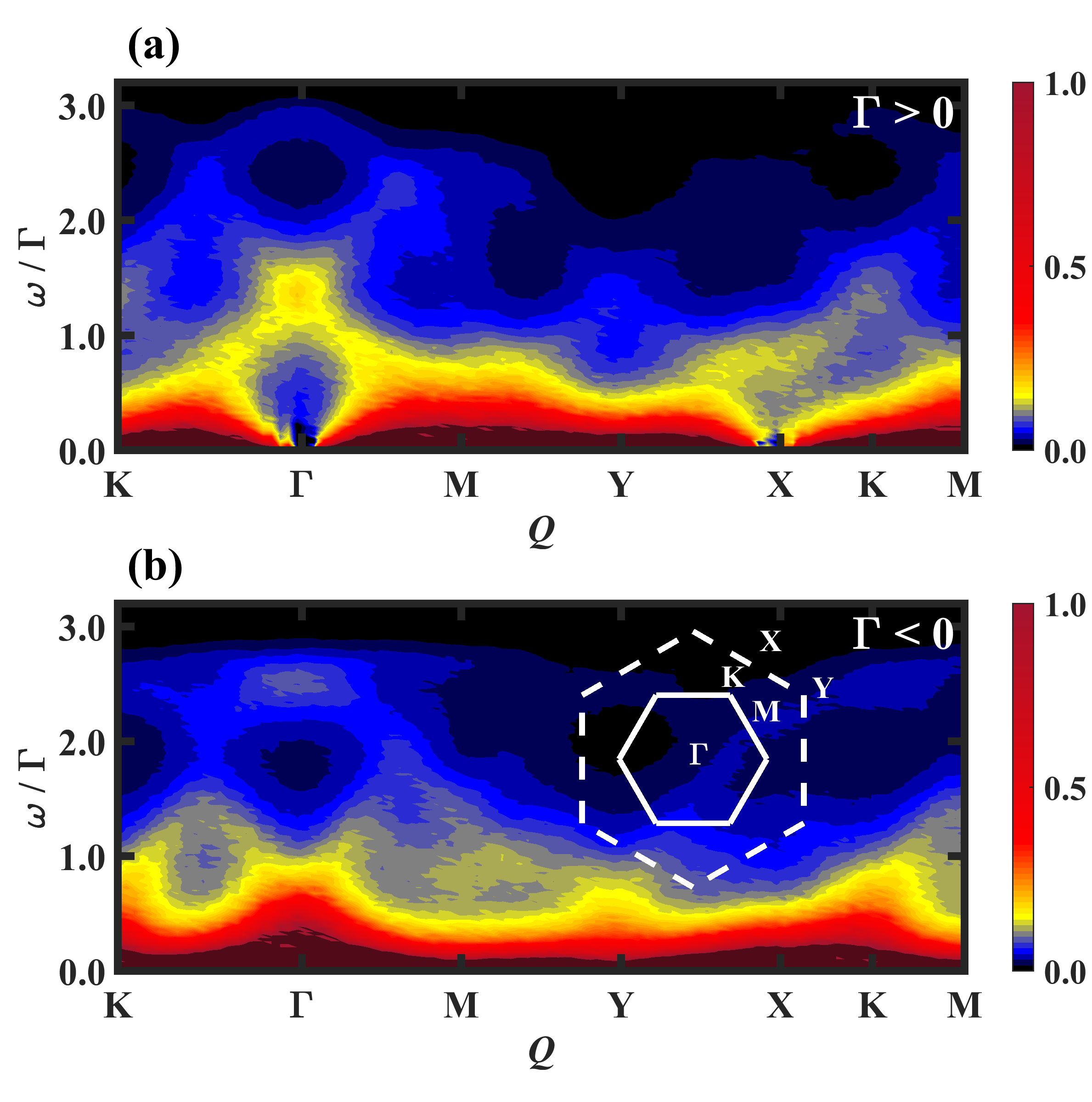
Figure 1: Trace of the dynamical magnetic structure factor $S\left({\bm{Q}},\omega\right)=\ \sum_{\alpha}{S^{\alpha\alpha}\left({\bm{Q}},\omega\right)}$ for (a) AFM ($\mathrm{\Gamma}>0$) (b) FM ($\mathrm{\Gamma}<0$) $\Gamma$-models along the Brillouin Zone path, ${\bm{K}}-{\bm{\Gamma}}-{\bm{M}}-{\bm{Y}}-{\bm{X}}-{\bm{K}}-{\bm{M}}$, as depicted in the inset.

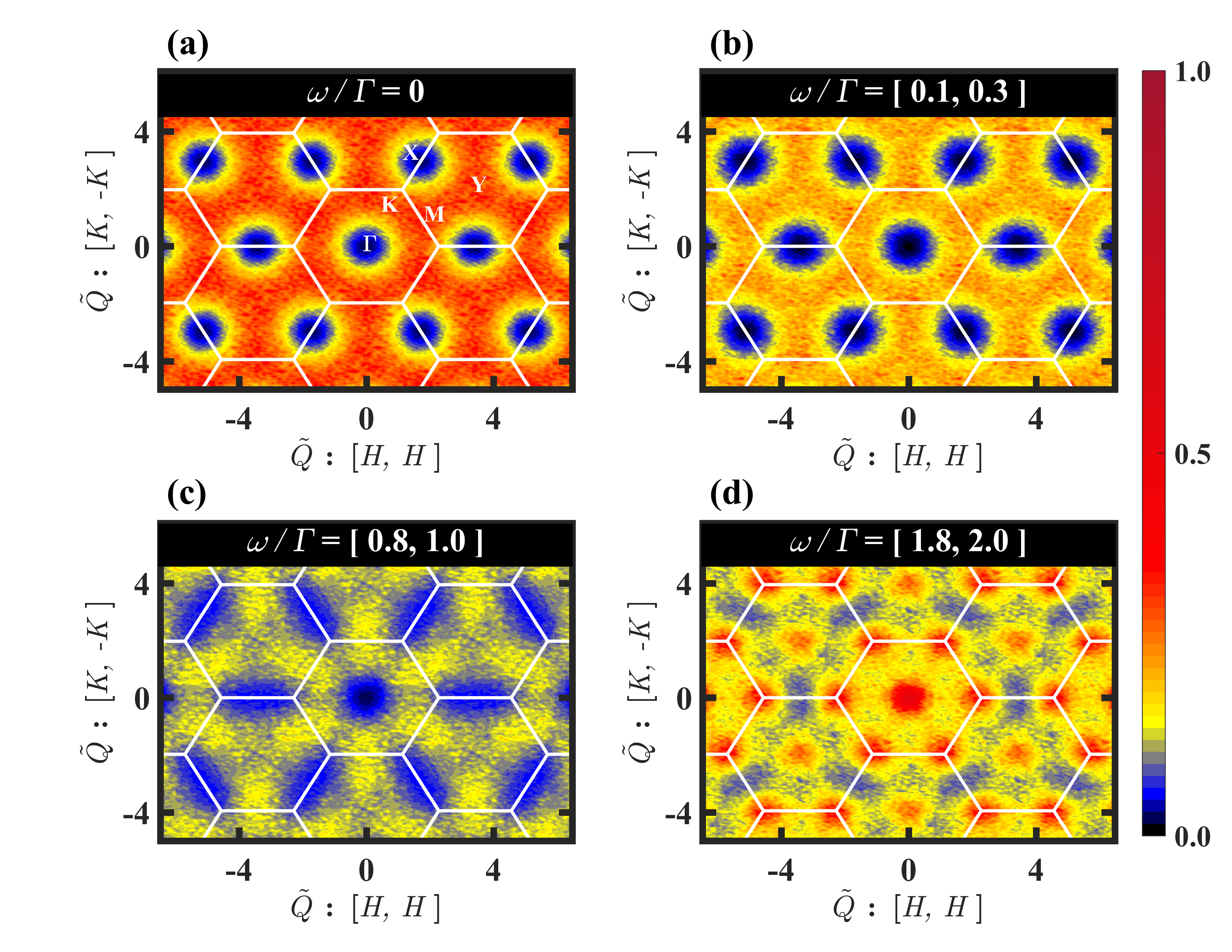
Figure 2: (a) Elastic component of the trace of the magnetic structure factor $S({\bm{Q}},\omega=0)$. (b-d) $S({\bm{Q}},\omega)$, integrated over finite energy cuts: (b) $\omega/\mathrm{\Gamma}=[0.1,0.3]$, (c) $\omega/\mathrm{\Gamma}$ = [0.8, 1.0] and (d)$\ \omega/\mathrm{\Gamma}$ = [1.8, 2.0].

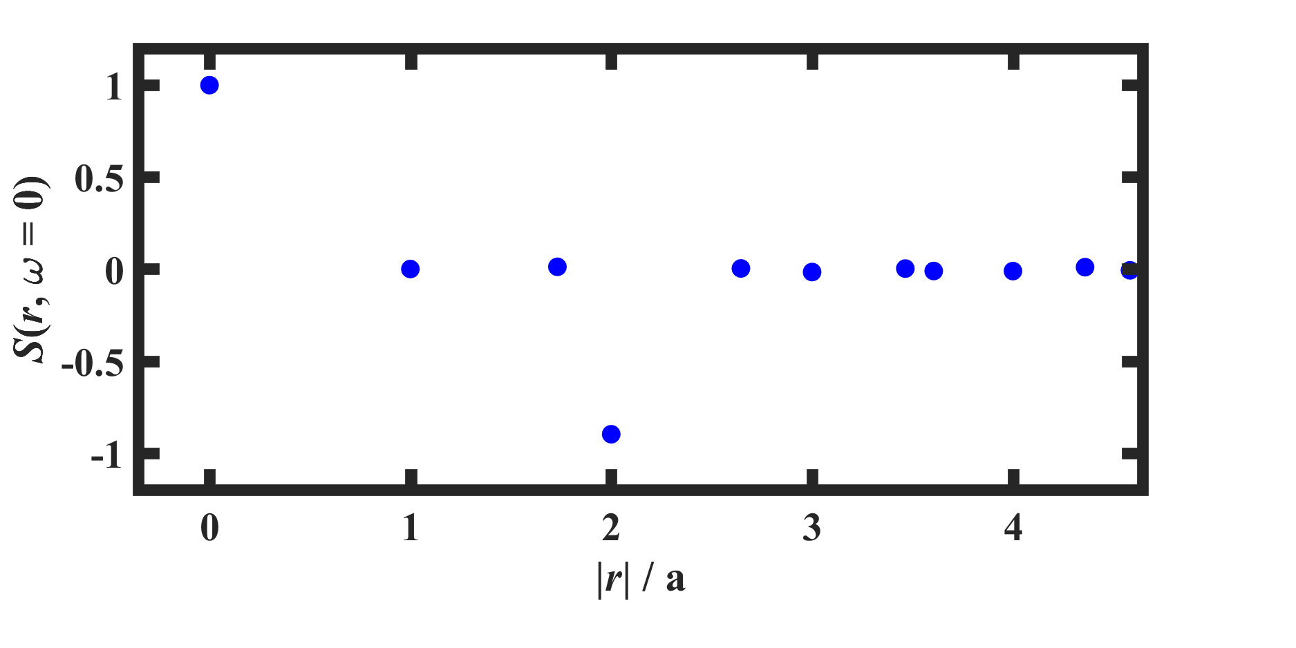
Figure 3: $S({\bm{r}},\omega=0)$ as a function of ${|{\bm{r}}|/a}$ (where $a$ is the lattice parameter) at $T=10^{-5}\Gamma$.

To gain more insight on the structure of the zero-energy modes, we also present the real space spin-spin correlation function, $S({\bm{r}},\omega)$, as a function of $\omega$ and $T$. Fig. 3 shows the elastic contribution $S({\bm{r}},\omega=0)$ for different distances up to fifth nearest neighbors (NN) and $T=10^{-5}\Gamma$ (calculations need to be done at finite $T$ to have fluctuations and be able to exploit the fluctuation-dissipation theorem). Remarkably, this is significant only for the on-site and for the third-nearest-neighbor ($|{\bm{r}}|/a=2$, where $a$ is the lattice parameter) correlation functions. The values obtained for other distances are smaller than the statistical error of the MC calculation. Therefore, the fast exponential decay of the elastic contribution indicates that the magnetic correlation length is of order $2a$.

A similar behavior is observed in the static real space spin-spin correlation function, $\tilde{S}^{\alpha\beta}({\bm{r}})=\left\langle S^{\alpha}_{\bm{0}}S^{\beta}_{\bm{r}}\right\rangle=\ \int{S^{\alpha\beta}\left({\bm{r}},\omega\right)d\omega}$, shown in Fig. 4. This figure also includes off-diagonal components of the spin-spin correlation function. In all the cases, the correlation function is significant only for distances $|{\bm{r}}|$ equal or smaller than the separation between third nearest neighbors (opposite sites of each hexagon). Moreover, a subset of the nine spin-spin correlator components $\alpha\beta$ vanishes, for any given $\bm{r}$. The form of the real space correlations, as depicted in Fig. 4, is well accounted for by considering the symmetries of the Hamiltonian, Eq. 1. To show this, we begin by considering the three ways in which one can decompose the honeycomb lattice into hexagon plaquettes, shown in Fig. 5. With each plaquette of a given decomposition we associate six spin components, one from each site around the plaquette. Specifically, a spin component is associated with a neighboring hexagon plaquette if it is of the same type as the bond connecting it with a neighboring plaquette of the same decomposition. There exist three symmetry operations Rousochatzakis and Perkins (2017), one for each plaquette decomposition, which correspond to $\pi$ spin rotations about an axis that depends on the sublattice which each spin belongs to. For example, the symmetry operation corresponding to the white plaquettes in Fig. 5, corresponds to a $\pi$-rotation about the $x$-axis for sublattices 1 and 4, about the $y$-axis for sublattices 2 and 5 and about the $z$-axis for sublattices 3 and 6. This transformation leaves the spin components $\{S_{1}^{x},S_{2}^{y},S_{3}^{z},S_{4}^{x},S_{5}^{y},S_{6}^{z}\}$ invariant (the subscript is the six sublattice index), while it changes the sign of the other ones. In appendix B, we show that these symmetries, which are also symmetries of the quantum model, result in vanishing correlations between spin components which are associated with plaquette of different decompositions, according to the rule we just described.

However, the spin-spin correlations are further restricted in the classical limit. Classically, the three components of each spin commute with each other, and as a result, one can define a local transformation that flips the sign of an individual spin component. The classical version of the $\Gamma$ model is invariant under a local symmetry transformation that changes the sign of one spin component of each of the six spins in a single hexagon plaquette. The spin component that changes sign is the one corresponding to the only bond which does not connect two spins in the same hexagon Rousochatzakis and Perkins (2017). For instance, the symmetry transformation changes the sign of $\{S_{1}^{x},S_{2}^{y},S_{3}^{z},S_{4}^{x},S_{5}^{y},S_{6}^{z}\}$ for a single white hexagon plaquette. This is the local symmetry that gives rise to the macroscopic degeneracy of the classical ground state manifold. Consequently, the correlation function $\left\langle S^{\alpha}_{\bm{0}}S^{\beta}_{\bm{r}}\right\rangle$ vanishes unless both $S_{0}^{\alpha}$ and $S_{\bm{r}}^{\beta}$ belong to the same single hexagon. This restricts correlations to third neighbor at most, and determines the specific components which have non zero correlations, as seen in Fig. 4. For example, only the diagonal components of the on-site correlations are non-zero, since different components of a given spin are associated with different plaquettes, and thus, uncorrelated. Similarly, the only other non-vanishing diagonal components of the spin-spin correlation function appears for third neighbors, e.g., for the white plaquette mentioned earlier we have only a finite $\left\langle S_{1}^{x}S_{4}^{x}\right\rangle$ in addition to the on-site correlation. Similar considerations restrict finite off-diagonal correlations to nearest and second nearest neighbors around one plaquette.

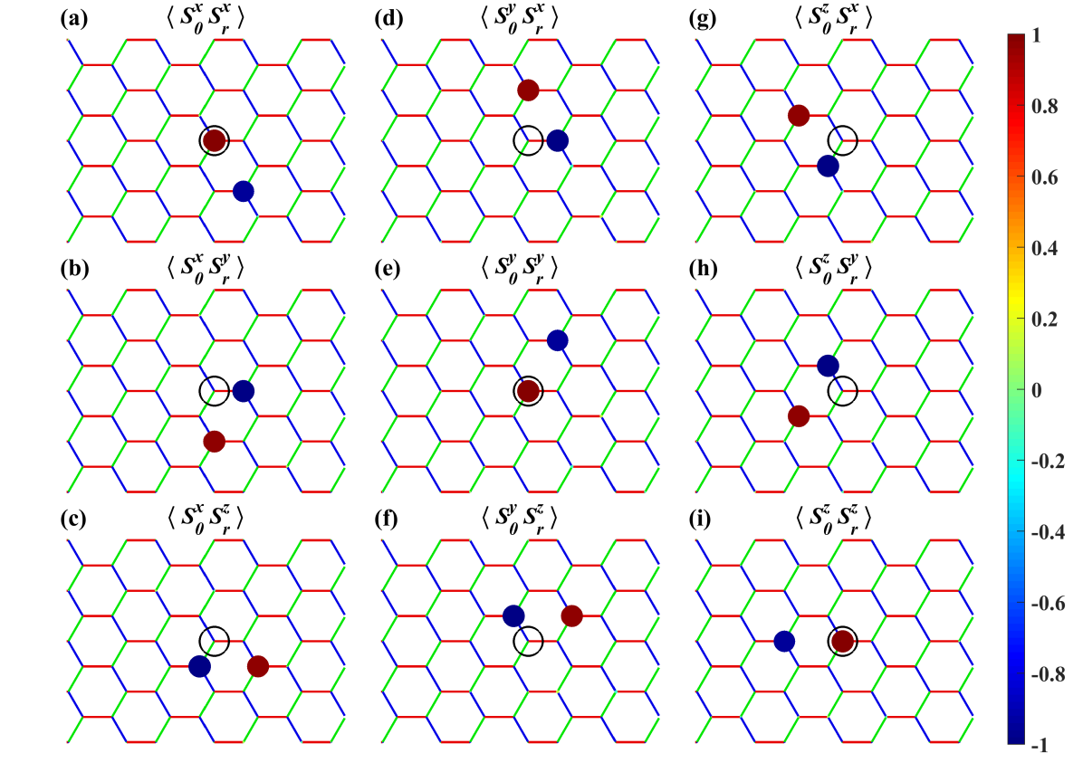
Figure 4: Static spin-spin correlation function, $\tilde{S}^{\alpha\beta}=\left\langle S^{\alpha}_{\bm{o}}S^{\beta}_{\bm{r}}\right\rangle=\ \int{S^{\alpha\beta}\left({\bm{r}},\omega\right)d\omega}$ mapped on the real-space lattice with respect to an arbitrary origin denoted by the cross ($\times$). The temperature of the simulation is $T=10^{-5}\Gamma$.

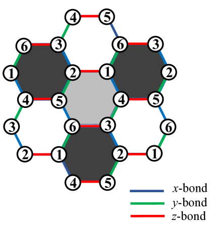
Figure 5: Six sublattice decomposition of the honeycomb lattice. We also show the three different decompositions of the lattice into isolated hexagonal plaquettes.

Fig. 6 shows the temperature and frequency dependence of $S\left({\bm{r}},\omega\right)$ for several values of ${\bm{r}}$. In agreement with the symmetry analysis given in Appendix B, $S\left({\bm{r}},\omega\right)$ vanishes for any frequency when ${\bm{r}}$ connects second nearest neighbor sites [see Figure 6 (b)]. The temperature dependence of $S\left({\bm{r}},\omega\right)$ for other values of ${\bm{r}}$ indicates a crossover from partially precessional to fully diffusive behavior at a temperature of order $\Gamma$. The temperature dependence of $S\left({\bm{Q}}={\bm{\Gamma}},\omega\right)$ shown in Figure 7 confirms this crossover, indicating that the system evolves continuously from a low-temperature ($T<\Gamma$) correlated liquid (classical $\Gamma$ liquid) to a high-temperature paramagnetic state.

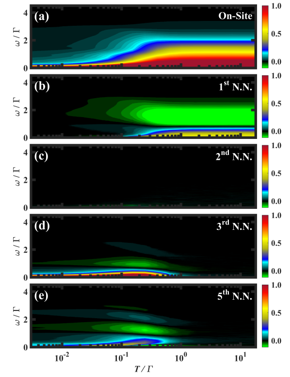
Figure 6: $S\left({\bm{r}},\omega\right)$ as a function of temperature and energy ($\hbar\omega$)for AFM ($\Gamma>0$) Gamma model. Panels (a), (d) and (e) show $-S\left({\bm{r}},\omega\right)$ for ${\bm{r}}$ connecting 1st, 3rd and 5th nearest-neighbor sites, respectively. Panel (b) shows $S\left({\bm{r}},\omega\right)$ for ${\bm{r}}$ connecting nearest-neighbor sites. Panel (c) shows that $S\left({\bm{r}},\omega\right)=0$ for ${\bm{r}}$ connecting second nearest neighbor sites.

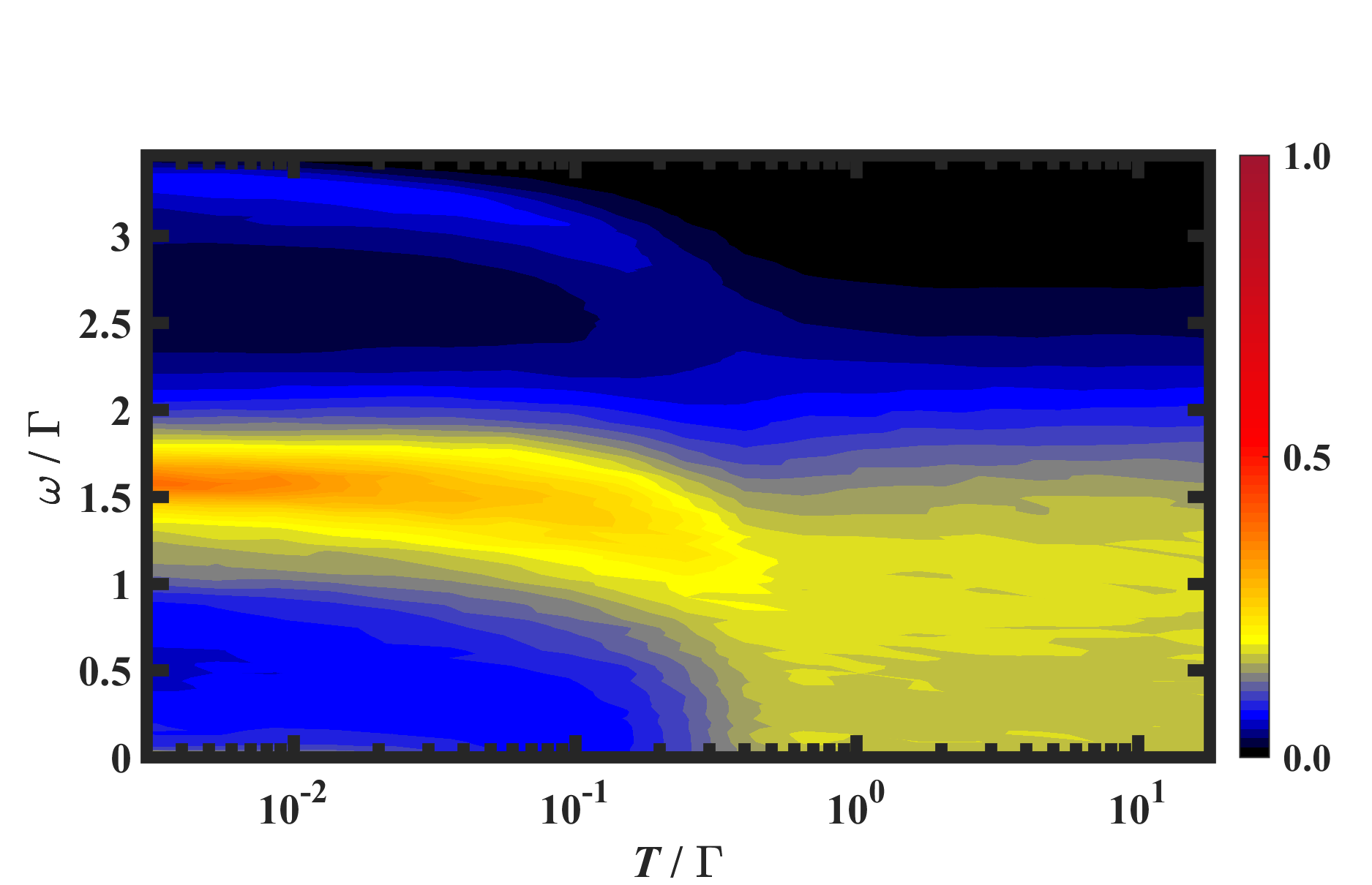
Figure 7: Temperature evolution of $S({\bm{Q}}={\bm{\Gamma}},\omega)$ for AFM ($\Gamma>0$) Gamma model.

III Langevin dynamics

Although, as noted in the previous section, neutron scattering experiments are faster than spin-lattice relaxation, a Langevin approach may still be used to analytically understand dynamic correlations in LL dynamics. The non-linear nature of Eq. (2) gives rise to strong relaxation due to inelastic processes, in addition to the more direct precessional dynamics. In other words, the fluctuating spins act as their own heat bath – leading to strong relaxation. At a phenomenological level, it is possible to capture the two types of spin dynamics in a generalized Langevin equation, where a linear term describes the spin relaxation, while precession is included in a residual non-linear term. We thus propose to study the stochastic dynamics of a system of soft classical spins Conlon and Chalker (2009) $S_{i}^{\alpha}$, given by

$$\frac{\partial S_{i}^{\alpha}}{\partial t}=g\epsilon_{\alpha\beta\gamma}S_{i}^{\beta}\frac{\partial H}{\partial S_{i}^{\gamma}}-\gamma\frac{\partial{H}}{\partial S_{i}^{\alpha}}+\eta_{i}^{\alpha},$$ (3)

where $i,j$ denote a site on a honeycomb lattice, $\alpha,\beta=x,y,z$ and the noise term $\eta_{i}^{\alpha}$ obeys

$$\left\langle\eta_{i}^{\alpha}(t)\eta_{j}^{\beta}(t^{\prime})\right\rangle=2\gamma T\delta_{ij}\delta_{\alpha\beta}\delta(t-t^{\prime}).$$ (4)

As described below, the unitless phenomenological parameters – $\gamma$ setting the relaxation rate and $g$ the precession rate – are chosen by comparing the dynamical correlations with the results of the LL simulation, while $T$ is simply the temperature. The spins are taken to be soft with mass $\Delta$, and with a general nearest neighbor spin interaction, $K_{ij}^{\alpha\beta}$, as given by the following Hamiltonian

$$H=\sum_{\alpha\beta}\sum_{\braket{ij}}K_{ij}^{\alpha\beta}S_{i}^{\alpha}S_{j}^{\beta}+\frac{\Delta}{2}\sum_{i\alpha}\left(S_{i}^{\alpha}\right)^{2},$$ (5)

The mass $\Delta$ is an additional, temperature dependent, phenomenological parameter which determines the average spin size $\braket{S_{i}^{2}}$. Quadratic Hamiltonians of this type are suitable for studying spin dynamics in cases where there is no long range order. We will apply this to the classical $\Gamma$ model, which has macroscopic degeneracy in its ground state, preventing long range order even at low temperatures. A similar treatment for the Kitaev model is given in the Appendix. Following a path integral formulation of the MSR approachMartin et al. (1973); De Dominicis and Peliti (1978); Wachtel and Orgad (2014), we write a generating functional for dynamical correlations as

$$Z\!=\!\left\langle\!\int DS\,|M|\,\delta\!\left(\frac{\partial S_{i}^{\alpha}}{\partial t}\!-\!g\epsilon_{\alpha\beta\gamma}S_{i}^{\beta}\frac{\partial H}{\partial S_{i}^{\gamma}}\!+\!\gamma\frac{\partial{H}}{\partial S_{j}^{\alpha}}\!-\!\eta_{i}^{\alpha}\right)\!\right\rangle_{\eta}\!,$$ (6)

where $\braket{\cdots}_{\eta}$ denotes averaging over the noise fluctuations $\eta$, and $M$ is a Jacobian matrix. For the model we consider here we may take the determinant $|M|=1$. Writing the delta function as an integral over $\hat{S}_{i}^{\alpha}$, and averaging over $\eta$, we obtain $Z=\int D\hat{S}\,DS\,e^{-\mathcal{S}}$ where the MSR action is given by

$$\mathcal{S} = -\int dt\left[\hat{S}_{i}^{\alpha}\left(\partial_{t}S_{i}^{\alpha}+\gamma K_{ij}^{\alpha\beta}S_{j}^{\beta}+\gamma\Delta S_{i}^{\alpha}\right)\right.$$ (7)

$$\left.\qquad\qquad+\gamma T(\hat{S}_{i}^{\alpha})^{2}-g\epsilon_{\alpha\beta\gamma}\hat{S}_{i}^{\alpha}S_{i}^{\beta}K_{ij}^{\gamma\delta}S_{j}^{\delta}\right],$$

Within this formalism it is possible to calculate dynamical correlation functions, using perturbation theory in $g$.

Figure 8: Feynman diagrams for the MSR formalism: (a) Bare response function. (b) Bare correlation function. (c) Precession vertex. (d) Self-energy diagram. (e) Perturbative expansion of the dressed correlation function, in powers of the self-energy $\Sigma$, see Eq. (15).

Zeroth order in $g$: When $g=0$, the dynamics is purely relaxational. The bare response Green’s function, defined as

$$\left(G_{0}(\omega)\right)_{ij}^{\alpha\beta}\equiv\left\langle\hat{S}_{i}^{\alpha}(-\omega)S_{j}^{\beta}(\omega)\right\rangle_{0},$$ (8)

is given by (its inverse)

$$\left(G^{-1}_{0}(\omega)\right)_{ij}^{\alpha\beta}=(-i\omega+\gamma\Delta)\delta_{\alpha\beta}\delta_{ij}+K_{ij}^{\alpha\beta}$$ (9)

We will represent this diagrammatically using Fig. 8a. Similarly, the bare correlation function is given by

$$\left(C_{0}(\omega)\right)_{ij}^{\alpha\beta}\equiv\left\langle S_{i}^{\alpha}(-\omega)S_{j}^{\beta}(\omega)\right\rangle_{0}=2\gamma T\left(G_{0}^{\dagger}(\omega)G_{0}(\omega)\right)_{ij}^{\alpha\beta}$$ (10)

Diagrammatically, this is represented in Fig. 8b where the noise vertex is represented by a dot, $\bullet=2\gamma T$.

In the pure $\Gamma$ model, which is defined by

$$K_{ij}^{\alpha\beta}=\left\{\begin{array}[]{cc}\Gamma&\alpha\neq\beta\neq\braket{ij}\\ 0&{\rm otherwise}\end{array}\right.,$$ (11)

the classical degrees of freedom can be divided into sectors – one for each hexagon. For example, as discussed in the previous section, going around one of the white hexagons in fig. 5, we can identify six spin components which interact only within themselves. Their dynamics is independent of the rest of the system, manifesting the macroscopic degeneracy of the classical system. We rename these degrees of freedom as follows,

$$\left\{S_{1}^{x},S_{2}^{y},S_{3}^{z},S_{4}^{x},S_{5}^{y},S_{6}^{z}\right\}\equiv\left\{\sigma_{1},\sigma_{2},\sigma_{3},\sigma_{4},\sigma_{5},\sigma_{6}\right\}.$$ (12)

The Hamiltonian, restricted to this sector, is given by

$$H_{\rm hexagaon}=\sum_{l=1}^{6}\left(\Gamma\sigma_{l}\sigma_{l+1}+\frac{\Delta}{2}\sigma_{l}^{2}\right).$$ (13)

The energy eigenvalues, which determine the relaxation rate, are $\varepsilon_{m}=2\Gamma\cos{\pi m}/{3}+\Delta,\quad m=1\dots 6$. Clearly, the model is stable only for $\Delta>2|\Gamma|$. The $g=0$ dynamical correlation function within these six spin components is given by

$$\left\langle\sigma_{l}(\omega)\sigma_{l^{\prime}}(\omega^{\prime})\right\rangle\!=\!\frac{1}{6}\!\sum_{m=1}^{6}\!\cos\!\left(\!\frac{\pi m(l-l^{\prime})}{3}\!\right)\frac{2\gamma T\,2\pi\delta(\omega+\omega^{\prime})}{\omega^{2}+\gamma^{2}\varepsilon_{m}^{2}},$$ (14)

while the correlation with spin components which do not appear in Eq. (12) is identically zero. $\Delta$ may be chosen so that $\braket{\sigma_{l}^{2}}$ is a constant; at the $g=0$ level $\Delta$ should obey $\braket{\sigma_{l}^{2}}=\sum_{m}(T/6\varepsilon_{m})=1$. Clearly, the dynamics for $g=0$ is purely relaxational, with a peak at $\omega=0$. Thus, $\gamma$ can be chosen such that Eq. (14) reproduces the width of the low energy peak as obtained in the LL simulations. Focusing on the dynamic structure factor $\braket{S^{\alpha}({\bf q},\omega)S^{\alpha}(-{\bf q},-\omega)}$, we note that for each hexagon $\braket{S^{x}_{l}S^{x}_{l^{\prime}}}\neq 0$ only for $l,l^{\prime}=1,4$, $\braket{S^{y}_{l}S^{y}_{l^{\prime}}}\neq 0$ only for $l,l^{\prime}=2,5$ and $\braket{S^{z}_{l}S^{z}_{l^{\prime}}}\neq 0$ only for $l,l^{\prime}=3,6$, in line with the symmetry consideration of the previous section and in Appendix B. In the anti-ferromagnetic $\Gamma$ model, the lowest eigenvalues is $\varepsilon_{3}=-2\Gamma+\Delta$. Noting that there are non-zero correlations only for $l-l^{\prime}=0,3$, we find that the contribution of this eigenvalue to the spectrum at $\bm{\Gamma}$ vanishes, and one would expect only the higher energy modes, i.e. faster relaxations, to contribute at this momentum. A similar argument holds for the low energy correlations at $\bm{X}$. Thus we find a depletion in the dynamic structure factor at $\bm{\Gamma}$ and $\bm{X}$, echoing the analysis of the zero modes in the previous section.

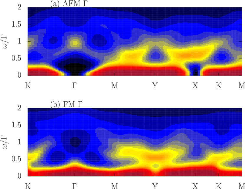
Figure 9: Dynamic structure factor as obtained from Eq. (15), for (a) the AFM $\Gamma>0$, and (b) the FM $\Gamma<0$ models. Here we have used $\gamma=0.12$, $\Delta=2.05\Gamma$ and $g^{2}T=0.04\Gamma$.

Perturbation theory in $g$. It is possible to treat the precession term using diagrammatic perturbation theory. We represent the symmetrized precession vertex by Fig. 8c. The dressed correlation function, $C_{ij}^{\alpha\beta}(\omega)$, can be calculated approximately, by summing over a subset of infinite diagrams, as shown in Fig. 8. Specifically, we approximate $C(\omega)$ by a product of two infinite series,

$$C(\omega)\approx 2\gamma T\left|G_{0}(\omega)\sum_{n=0}^{\infty}\left(\Sigma(\omega)G_{0}(\omega)\right)^{n}\right|^{2},$$ (15)

where the ‘self energy’ $\Sigma$ is calculated to leading order in $g$. The self energy term for the $\Gamma$ model dynamics mixes different sectors, and therefore its calculation must be done in Fourier space. However, the procedure is no different than in quantum field theory, once the appropriate Feynman rules are determined. Fig. 9 shows the resulting dynamic structure factor. Eq. (14), obtained for $g=0$, qualitatively accounts for the low frequency features, including the depletion at $\bm{\Gamma}$ and $\bm{X}$ in the AFM case. The main qualitative effect of finite $g>0$ on the dynamic structure factor, is the addition of correlations peaked at finite frequency, due to the precession of the spins. In Appendix C we describe the calculation for the Kitaev model, which is simpler, and can be done in real space. Furthermore, the closed form result for the Kitaev model shows that the self energy is larger for the mode which is suppressed at low energies. Similar behavior is observed in Fig. 9 for the $\Gamma$ model, where the precession features appear at finite frequency at the same momentum positions with depleted low energy correlations. Besides the qualitative effect of precessional dynamics, a finite $g$ is also expected to renormalize the values of $\gamma$ and $\Delta$ required to fit the numerical data obtained at a given temperature.

IV Dynamics of the spin-$\frac{1}{2}$ model

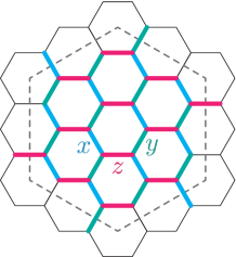
Figure 10: (color online): Finite-size honeycomb clusters with 24 spins and periodic boundary conditions. Bonds along the three different directions are labeled as the $x$, $y$, and $z$ bond, which are along -60^∘, 60^∘, and horizontal directions, respectively.

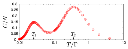
Figure 11: (color online): Specific heat $C/N$ of the AFM $\Gamma$ model on the $N=24$ site cluster Catuneanu et al. (2018), calculated by the typical pure quantum states approach Hams and De Raedt (2000); Sugiura and Shimizu (2013). There are two maxima in the temperature dependence of $C/N$. The error bars are the standard errors estimated by 32 random initial vectors.

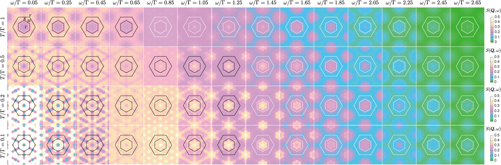
Figure 12: (color online): Equi-energy slices of the dynamical spin structure factors of the $\Gamma>0$ model. The momentum dependence of the equi-energy slices is shown by changing temperature and frequency. From the top row to the bottom row, the equi-energy slices of the dynamical spin structure factors are shown at $T/\Gamma=1$, $0.5$, $0.2$, and $0.1$. The equi-energy slices are prepared by averaging the spectra within an energy window whose width is 0.1. For visibility, the dynamical spin structure factors at discrete momenta obtained by the simulation are interpolated. Here, the broadening factor $\eta/\Gamma=0.02$ is used (see Appendix D for the definition of $\eta$).

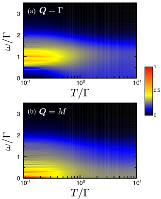
Figure 13: (color online): Temperature evolution of $S(\mbox{\boldmath$Q$}=\Gamma,\omega)$ and $S(\mbox{\boldmath$Q$}=M,\omega)$ for the $\Gamma>0$ model.

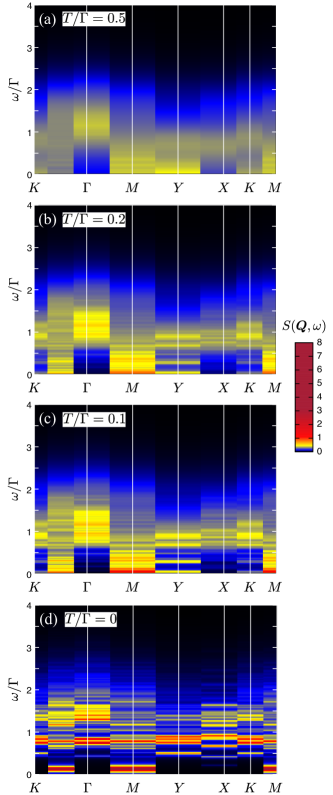
Figure 14: (color online): Dynamical spin structure factors of the $S=1/2$ AFM $\Gamma$ model at (a) $T=0.5$, (b) $T=0.2$, (c) $T=0.1$, and (d) $T=0$, along symmetry lines. For visibility, the broadening factor $\eta/\Gamma=0.02$ is used (see Appendix D for the definition of $\eta$).

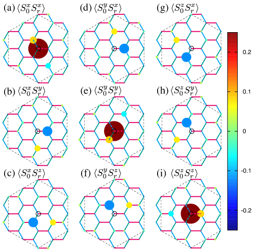
Figure 15: (color online): Real-space static spin-spin correlation function, $\langle{S}^{\alpha}_{\mbox{\boldmath$0$}}{S}^{\beta}_{\mbox{\boldmath$r$}}\rangle$ $(\alpha,\beta=x,y,z)$, of the $S=1/2$ $\Gamma>0$ model on the 24 site cluster with periodic boundary condition, at $T=0$. The location of the origin $\mathrm{𝟎}$ is denoted by the open circle ($\circ$). The radiuses of the closed circles at $r$ represent the amplitude of $|\langle{S}^{\alpha}_{\mbox{\boldmath$0$}}{S}^{\beta}_{\mbox{\boldmath$r$}}\rangle|$, while the color of the closed circles shows $\langle{S}^{\alpha}_{\mbox{\boldmath$0$}}{S}^{\beta}_{\mbox{\boldmath$r$}}\rangle$. Within numerical accuracy, there is no spin-spin correlation represented by a circle with a radius smaller than the width of the solid lines representing the bonds.

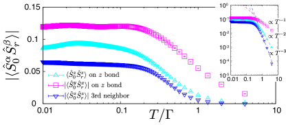
Figure 16: (color online): Temperature dependence of static spin-spin correlations of the AFM $\Gamma$ model on the 24 site cluster. Here, the error bars, which are smaller than or comparable to the symbol size, are the standard errors estimated by several random initial vectors.

Using the exact-diagonalization method, described in Ref. Yamaji et al., 2018 and Appendix D, we study the finite-temperature dynamical spin structure factors of the $S=1/2$ AFM $\Gamma$ model. Here, we use a 24 site cluster with periodic boundary conditions, illustrated in Fig. 10. As explained below, the dynamical spin structure factor of the quantum model shows a gradual classical-to-quantum crossover when the temperature is decreased.

Before going into details of the quantum spin dynamics of the $\Gamma$ model, we summarize the energy scale of the quantum $S=1/2$ $\Gamma$ model. As shown in Ref. Catuneanu et al., 2018 and Fig. 11, there are two temperature scales given by the peaks in the temperature dependence of the specific heat. The higher-temperature peak appears around $T_{2}/\Gamma\sim 0.4$ and the lower-temperature peak emerges below $T_{1}/\Gamma\lesssim 0.03$. The two peak structure in the temperature dependence of the specific heat has been found in the Kitaev model Nasu et al. (2015) and in the proximity of the Kitaev’s spin liquid Yamaji et al. (2016), although the balance of the entropy released by these two peaks is different from that of the $\Gamma$ model.

In Fig. 12, the momentum dependence of the equi-energy slices of $S(\mbox{\boldmath$Q$},\omega)$ are shown by changing temperature and frequency. The equi-energy slices are prepared by averaging the spectra within an energy window whose width is 0.1. The momentum dependence is numerically interpolated for visibility without changing the simulation results at the discrete momenta $Q$ compatible with the finite size cluster. At $T/\Gamma=1>T_{2}/\Gamma\sim 0.4$, almost momentum-independent behaviors of $S(\mbox{\boldmath$Q$},\omega)$ are found except around $\Gamma$ point, where spectral weight is suppressed for $\omega/\Gamma<1$ and is shifted to the high energy region $\omega/\Gamma>1$. Below $T/\Gamma=0.5\sim T_{2}/\Gamma$, the suppression of the low-energy spectral weight (or relaxational dynamics) at $\Gamma$ and $X$ points becomes notable, which is consistent with the classical dynamics.

To examine the temperature dependence of the low energy spectral weight, we show the temperature evolution of $S(\mbox{\boldmath$Q$}=\bm{\Gamma},\omega)$ in comparison with $S(\mbox{\boldmath$Q$}=\bm{M},\omega)$ in Fig.13. Below the high temperature scale $T/\Gamma\sim 0.4$, $S(\mbox{\boldmath$Q$}=\bm{\Gamma},\omega)$ shows reduced spectral weight in the low energy region below $\omega/\Gamma\sim 0.5$, while $S(\mbox{\boldmath$Q$}=\bm{M},\omega)$ shows substantial spectral weight in the low energy region. We further note that the Fourier transformation of $S(\mbox{\boldmath$Q$},\omega)$, $S(\mbox{\boldmath$r$}_{\ell m},\omega)$, also satisfies the symmetry properties at finite temperatures, as discussed in section II.

For closer comparison with the classical dynamics, we show $S(\mbox{\boldmath$Q$},\omega)$ at $T/\Gamma=0.5$, $0.2$, $0.1$, and $0$ along symmetry lines in Fig.14. In addition to the suppression of the low-energy spectral weight at $\Gamma$ and $X$ points, which is in common with the classical spin dynamics, the low-energy spectral weight for $\omega/\Gamma\lesssim 0.5$ decreases at $K$ and $Y$ upon cooling. This suppression at the $K$ and $Y$ points is characteristic of the $S=1/2$ $\Gamma$ model.

To gain insight into the difference between the quantum and classical dynamics at the $K$ and $Y$ points, we examine the static spin-spin correlation function at zero temperature. In Fig.15, $\langle{S}^{\alpha}_{\mbox{\boldmath$0$}}{S}^{\beta}_{\mbox{\boldmath$r$}}\rangle$ $(\alpha,\beta=x,y,z)$ are shown in the 24 site cluster with the periodic boundary condition. These correlators in the quantum model are very similar to the static correlation functions of the classical model, as shown in Fig. 4. Due to the symmetry of the $\Gamma$ model, the static spin-spin correlation functions are zero for many spin pairs. However, there are differences among them: For example, there exist finite nearest-neighbor correlations $\langle{S}^{\alpha}_{\mbox{\boldmath$0$}}{S}^{\beta}_{\mbox{\boldmath$r$}}\rangle$ $(\alpha,\beta=x,y,z)$ for $\alpha=\beta$ and the additional second nearest-neighbor correlations for $\alpha\neq\beta$. The fact that these correlations are finite, while they are absent in the classical limit, indicates that quantum fluctuations are important even when $T>T_{1}$.

The most significant difference is the nearest-neighbor correlations for $\alpha=\beta$, which are zero in the classical model due to the the local symmetry discussed in Sec. II. The nearest-neighbor ferromagnetic correlations in the real space hinder the antiferromagnetic low-energy fluctuations at the $Y$ and $K$ points in the momentum space. As a result, these correlations harden the spin fluctuations at these momenta. In other words, these correlations suppress the relaxational dynamics and introduce the quasi-collective precessional dynamics at these momenta.

A quantitative description of the classical-quantum crossover is obtained by examining temperature dependence of the typical static spin-spin correlation functions shown in Fig. 16. While the off-diagonal nearest-neighbor correlations $\langle{S}^{\alpha}_{\mbox{\boldmath$0$}}{S}^{\beta}_{\mbox{\boldmath$r$}}\rangle$ on the $\gamma$ bond, where $(\alpha,\beta,\gamma)$ is a permutation of $(x,y,z)$, are dominant at temperatures above and around $T_{2}/\Gamma\sim 0.4$, the diagonal nearest-neighbor correlations $\langle{S}^{\alpha}_{\mbox{\boldmath$0$}}{S}^{\alpha}_{\mbox{\boldmath$r$}}\rangle$ start to saturate upon cooling for $T<T_{2}$. Therefore, the classical precessional dynamics due to the off-diagonal nearest-neighbor correlations governs the dynamics for $T\gtrsim T_{2}$. On the other hand, the emergent quantum dynamics is generated by the diagonal nearest-neighbor correlations for $T<T_{2}$. Here, we note that dominance of the off-diagonal nearest-neighbor correlations originates from their Curie-like temperature dependence in the high temperature region, which is evident in the inset of Fig. 16, while temperature dependence of the diagonal nearest-neighbor and third nearest-neighbor correlations shows $T^{-2}$ and $T^{-3}$ scaling, respectively. In Appendix E we show how these power-law behaviors can be obtained using a high temperature expansion.

V Discussion

In this work, we investigated classical and quantum dynamics of the $\Gamma$ model, the bond-dependent symmetric and anisotropic spin interaction on the honeycomb lattice. Such exchange interaction arises in strongly spin-orbit-coupled Mott insulators, in addition to the usual Heisenberg and Kitaev (the bond-dependent Ising) interactionsRau et al. (2014, 2016). There exist a number of so-called “Kitaev materials” such as $\alpha,\beta,\gamma$-Li₂IrO₃ and $\alpha$-RuCl₃, where the Kitaev interaction, if dominant, may lead to a quantum spin liquid phase. However, the strength of the $\Gamma$ interaction can be as large as that of the Kitaev interaction, especially in the case of $\alpha$-RuCl₃, according to recent ab initio computationsWinter et al. (2016). The presence of other interactions has been regarded as an obstacle for realizing the quantum spin liquid ground state in this class of materials.

On the other hand, the $\Gamma$ interaction is also highly frustrated at the classical level, just like the Kitaev model. Given that the strength of this interaction is significant in some materials, the nature of the quantum ground state of the $\Gamma$ model is highly relevant for the interpretation of the experiments. In the case of $\alpha$-RuCl₃, for example, it has been speculated that the scattering continuum seen in recent neutron scattering experiment may come from a nearby quantum spin liquid even though the actual ground state is a magnetically ordered state Banerjee et al. (2016, 2017). The magnetic order can be suppressed by external in-plane magnetic field and the resulting paramagnetic state is speculated to be a field-induced quantum spin liquidSears et al. (2017); Hentrich et al. (2018); Wolter et al. (2017). Currently it is highly debated whether the Kitaev interaction or other interactions or both could be responsible for the formation of a putative quantum spin liquid ground state.

In the present work, we focused on the $\Gamma$ interaction and pointed out the similarity to the Kitaev model, in the correspondence between classical and quantum dynamics. We showed that the zero mode structure of the highly degenerate manifold of the classical ground states is reflected in the classical dynamical spin structure factor. In addition, we clarified different roles of relaxational and precessional dynamics in the dynamical spin structure factor of the classical model. Remarkably this feature survives in the quantum model down to very low energy scales. This would imply that the full degenerate manifold of the classical states are participating in quantum fluctuations down to very low energy scales. This situation resembles the results of the Kitaev model, obtained in a previous study Samarakoon et al. (2017), where the quantum dynamical spin structure factor is qualitatively similar to the classical results down to low energies above the small flux gap in the underlying spin liquid ground state. This correspondence in the Kitaev model was apparent even in the temperature/energy window where the underlying low energy degrees of freedom are Majorana fermions, not the semiclassical spins. Since the quantum $\Gamma$ model is not exactly solvable, we do not know the true quantum ground state at zero temperature. It has been suggested that order by quantum disorder leads to a symmetry-broken stateRousochatzakis and Perkins (2017). The resemblance to the Kitaev model, however, suggests that the quantum ground state of the $\Gamma$ model may also be a quantum spin liquid, which results from the “collapse” of the degenerate classical manifold. Such conclusion may also be consistent with a recent DMRG computation of the same modelGohlke et al. (2018), where the ground seems to be a highly correlated quantum paramagnet. If the $\Gamma$ model can indeed support a quantum spin liquid ground state, the presence of this interaction in real materials may not necessarily be an obstruction for the realization of the quantum spin liquid ground state. The firm answer to this question would require further studies of the quantum and classical models with both the Kitaev and $\Gamma$ interactions.

Appendix A Zero Modes Structure

The momentum space distribution of the zero modes can be derived from the set of constraints satisfied by the ground state manifold. As reported by Rousochatzakis and Perkins Rousochatzakis and Perkins (2017), the classical ground state of the AFM $\Gamma$ model satisfies the following constraints on each bond of the lattice:

$$S^{x}_{1} = -S^{y}_{2},\;\;\;{\rm and}\;\;\;S^{y}_{1}=-S^{x}_{2}\;\;\;{\rm for}\;\;\;{z-{\rm bonds}},$$

$$S^{x}_{1} = -S^{z}_{2},\;\;\;{\rm and}\;\;\;S^{z}_{1}=-S^{x}_{2}\;\;\;{\rm for}\;\;\;{y-{\rm bonds}},$$

$$S^{y}_{1} = -S^{z}_{2},\;\;\;{\rm and}\;\;\;S^{z}_{1}=-S^{y}_{2}\;\;\;{\rm for}\;\;\;{x-{\rm bonds}},$$ (16)

where $1$ and $2$ denote the two sites on the given bond. Eq. 17 implies that the following identities hold for any ground state configuration:

$$S^{x}_{A} = -S^{y}_{B},\;\;\;S^{y}_{A}=-S^{x}_{B},\;\;\;S^{x}_{A}=-S^{z}_{B},$$

$$S^{z}_{A} = -S^{x}_{B},\;\;\;S^{y}_{A}=-S^{z}_{B},\;\;\;S^{z}_{A}=-S^{y}_{B},$$ (17)

where $S^{\mu}_{A}=\sum_{j\in A}S^{\mu}_{j}$ and $S^{\mu}_{B}=\sum_{j\in B}S^{\mu}_{j}$ and ($A$, $B$) denote the two sublattices of the honeycomb lattice shown in Fig. 17 (a). The conditions (17) lead to $S^{x}_{A}=S^{y}_{A}=S^{z}_{A}$, $S^{x}_{B}=S^{y}_{B}=S^{z}_{B}$ and $S^{\mu}_{A}+S^{\mu}_{B}=0$, implying that the ground states of the classical AFM $\Gamma$-model have no zero momentum component. This simple analysis proves the absence of elastic ($\omega=0$) spectral weight at the ${\bm{\Gamma}}$ point.

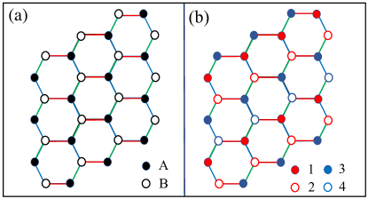
Figure 17: (a) Two-sublattice decomposition of the honeycomb lattice. (b) Four-sublattice decomposition of the honeycomb lattice.

Our next goal is to demonstrate the absence of elastic weight at the ${\bm{X}}$ points. For this purpose, we divide the honeycomb lattice into four sublattices, as shown in Fig. 17 (b). Without loss of generality, we prove the statement for one of the three ${\bm{X}}$ points, say ${\bm{X}}_{1}$. The C₆ symmetry of the honeycomb lattice guarantees that the result is the same for ${\bm{X}}_{2}$ and ${\bm{X}}_{3}$. The ${\bm{X}}_{1}$ component of a given spin configuration is:

$$S^{\mu}_{{\bm{X}}_{1}}=\frac{2}{\sqrt{N}}\left[S^{\mu}_{1}+S^{\mu}_{2}-S^{\mu}_{3}-S^{\mu}_{4}\right]$$ (18)

where $S^{\mu}_{r}=\sum_{j\in r}S^{\mu}_{j}$ and the integer index $1\leq r\leq 4$ denotes each of the six sublattices and $N$ is the total number of sites. From the general ground state condition (17), we obtain:

$$S^{y}_{1} = -S^{z}_{2},\;\;\;S^{z}_{1}=-S^{y}_{2},\;\;\;S^{x}_{1}=-S^{y}_{4},$$

$$S^{y}_{1} = -S^{x}_{4},\;\;\;S^{z}_{1}=-S^{x}_{4},\;\;\;S^{x}_{1}=-S^{z}_{4},$$

$$S^{x}_{2} = -S^{y}_{3},\;\;\;S^{y}_{2}=-S^{x}_{3},\;\;\;S^{x}_{2}=-S^{z}_{3},$$

$$S^{z}_{2} = -S^{x}_{3},\;\;\;S^{y}_{3}=-S^{z}_{4},\;\;\;S^{z}_{3}=-S^{y}_{4}.$$ (19)

These identities give $S^{x}_{1}=-S^{y}_{4}=S^{z}_{3}=S^{x}_{2}$, $S^{x}_{3}=-S^{y}_{2}=S^{z}_{1}=-S^{x}_{4}$, implying that $S^{x}_{{\bm{X}}_{1}}=0$. Similarly, Eq. 19 leads to $S^{y}_{1}=-S^{z}_{2}=S^{x}_{3}=-S^{y}_{2}$, $S^{z}_{1}=-S^{x}_{4}=S^{y}_{1}=-S^{z}_{2}$, $S^{z}_{3}=-S^{y}_{4}=S^{x}_{1}=-S^{z}_{4}$, implying that $S^{y}_{{\bm{X}}_{1}}=S^{z}_{{\bm{X}}_{1}}=0$. In other words, the ground state configurations of the AFM $\Gamma$ model have no ${\bm{\Gamma}}$ or ${\bm{X}}_{\mu}$ ($\mu=1,2,3$) components, implying the absence of elastic ($\omega=0$) spectral weight at any of those wave vectors.

Appendix B Symmetry analysis of $S^{\alpha\beta}(\bm{r},\bm{r^{\prime}},\omega)$

Here we derive selection rules of the real space dynamical spin structure factor of ${\cal H}$ for arbitrary spin $S$. For this purpose, we introduce the six sublattice decomposition of the honeycomb lattice that is depicted in Fig. 5 Rousochatzakis and Perkins (2017). We demonstrate that six out of the nine components of the real space and real time magnetic structure factor,

$$S^{\alpha\beta}({\bm{r}},{\bm{r}}^{\prime},t)=\langle S^{\alpha}_{\bm{r}}(0)S^{\beta}_{{\bm{r}}^{\prime}}(t)\rangle,$$ (20)

always vanish as a consequence of the Hamiltonian symmetries that we discuss next.

It was noticed in Ref. Rousochatzakis and Perkins, 2017 that the Gamma model (1) is invariant under a set of three spin transformations acting on each of the six sublattices depicted in Fig. 5.

• If we decompose the full lattice into the white hexagons shown in Fig. 5, the Hamiltonian ${\cal H}$ is invariant under the symmetry operation:

  $${\cal R}_{a}=\prod_{i\in\{1,4\}}C_{2x}(i)\prod_{i^{\prime}\in\{2,5\}}C_{2y}(i^{\prime})\prod_{i^{\prime\prime}\in\{3,6\}}C_{2z}(i^{\prime\prime}).$$ (21)

• Similarly, a lattice decomposition into the dark grey hexagons shown in Fig. 5 reveals the symmetry operation:

  $${\cal R}_{b}=\prod_{i\in\{6,5\}}C_{2x}(i)\prod_{i^{\prime}\in\{3,4\}}C_{2y}(i^{\prime})\prod_{i^{\prime\prime}\in\{1,2\}}C_{2z}(i^{\prime\prime}).$$ (22)

• Finally, a decomposition into the light grey hexagons in Fig. 5 leads to the symmetry operation:

  $${\cal R}_{c}=\prod_{i\in\{2,3\}}C_{2x}(i)\prod_{i^{\prime}\in\{1,6\}}C_{2y}(i^{\prime})\prod_{i^{\prime\prime}\in\{4,5\}}C_{2z}(i^{\prime\prime}).$$ (23)

We will derive now selection rules based on these symmetries. Given that these selection rules are excatly the same for any pair of sites ${\bm{r}}$ and ${\bm{r}}^{\prime}$ belonging to a given pair of sublattices $\nu$ and $\nu^{\prime}$, we will use the notation $\langle S^{\alpha}_{\nu}(0)S^{\beta}_{\nu^{\prime}}(t)\rangle$ instead of $\langle S^{\alpha}_{\bm{r}}(0)S^{\beta}_{{\bm{r}}^{\prime}}(t)\rangle$. We start by considering spin-spin correlators between sites on the same sublattice, i.e., both ${\bm{r}}$ and ${\bm{r}}^{\prime}$ belong to the same sublattice $\nu$ ($1\leq\nu\leq 6$). Off-diagonal contributions involve a product of two different spin components $S^{\alpha}_{\nu}$ and $S^{\beta}_{\nu}$ with $\alpha\neq\beta$. Because both spin operators belong to the same sublattice, they rotate about the same axis under the transformations ${\cal R}_{a}$, ${\cal R}_{b}$ or ${\cal R}_{c}$. We can always choose the transformation ${\cal R}^{\;}_{\eta}$ that corresponds to a $\pi$ rotation about the $\alpha$-axis. Given that $\alpha$ and $\beta$ are different components, we have:

$${\cal R}^{\dagger}_{\eta}S^{\alpha}_{\nu}{\cal R}^{\;}_{\eta}=S^{\alpha}_{\nu},\;\;\;{\rm and}\;\;\;{\cal R}^{\dagger}_{\eta}S^{\beta}_{\nu}{\cal R}^{\;}_{\eta}=-S^{\beta}_{\nu},$$ (24)

implying that

$$\langle S^{\alpha}_{\nu}(0)S^{\beta}_{\nu}(t)\rangle = {\rm Tr}[e^{-({\cal H}/k_{B}T)}S^{\alpha}_{\nu}(0)S^{\beta}_{\nu}(t)]$$ (25)

$$= {\rm Tr}[{\cal R}^{\dagger}_{\eta}e^{-({\cal H}/k_{B}T)}S^{\alpha}_{\nu}(0)S^{\beta}_{\nu}(t){\cal R}^{\;}_{\eta}]$$

$$= {\rm Tr}[e^{-({\cal H}/k_{B}T)}{\cal R}^{\dagger}_{\eta}S^{\alpha}_{\nu}(0){\cal R}^{\;}_{\eta}{\cal R}^{\dagger}_{\eta}S^{\beta}_{\nu}(t){\cal R}^{\;}_{\eta}]$$

$$= -\langle S^{\alpha}_{\nu}(0)S^{\beta}_{\nu}(t)\rangle=0.$$

By using this result and and from the Hamiltonian symmetry under the product of a spin rotation by $2\pi/3$ about the $[111]$ direction and an orbital rotation by the same angle along the direction perpendicular to the plane of the honeycomb lattice, we obtain:

$$\langle S^{\alpha}_{\nu}(0)S^{\beta}_{\nu}(t)\rangle=\delta_{\alpha\beta}\langle S^{z}_{\nu}(0)S^{z}_{\nu}(t)\rangle$$ (26)

for general values of $\alpha$ and $\beta$.

We consider now the spin-spin correlator (20) for ${\bm{r}}$ and ${\bm{r}}^{\prime}$ belonging to different sublattices with the same parity ($\nu\neq\nu^{\prime}$ and $\nu+\nu^{\prime}$ even). For any diagonal component ($\mu=\nu$), it is easy to verify that at least one of the three symmetry transformations, ${\cal R}_{a}$, ${\cal R}_{b}$ or ${\cal R}_{c}$ changes the sign of only one of the two spin operators:

$${\cal R}^{\dagger}_{\eta}S^{\alpha}_{\nu}{\cal R}^{\;}_{\eta}=\pm S^{\alpha}_{\nu},\;\;\;{\rm and}\;\;\;{\cal R}^{\dagger}_{\eta}S^{\alpha}_{\nu^{\prime}}{\cal R}^{\;}_{\eta}=\mp S^{\alpha}_{\nu^{\prime}}.$$ (27)

Here $\eta=a,b$ or $c$ denotes the transformation that satisfies (27). Note that ${\cal R}^{\dagger}_{\eta}={\cal R}^{\;}_{\eta}$. Once again, following the same procedure as in Eq. (25), we obtain

$$\langle S^{\alpha}_{\nu}(0)S^{\alpha}_{\nu^{\prime}}(t)\rangle=0.$$ (28)

By using a similar procedure, we can demonstrate that three, out of the six, off-diagonal correlators between different sublattices with the same parity are also equal to zero:

$$\langle S^{x}_{1}(0)S^{y}_{3}(t)\rangle = \langle S^{y}_{1}(0)S^{z}_{3}(t)\rangle=\langle S^{z}_{1}(0)S^{x}_{3}(t)\rangle=0,$$

$$\langle S^{x}_{1}(0)S^{z}_{5}(t)\rangle = \langle S^{z}_{1}(0)S^{y}_{5}(t)\rangle=\langle S^{y}_{1}(0)S^{x}_{5}(t)\rangle=0,$$

$$\langle S^{y}_{2}(0)S^{z}_{4}(t)\rangle = \langle S^{z}_{2}(0)S^{x}_{4}(t)\rangle=\langle S^{x}_{2}(0)S^{y}_{4}(t)\rangle=0,$$

$$\langle S^{y}_{2}(0)S^{x}_{6}(t)\rangle = \langle S^{x}_{2}(0)S^{z}_{6}(t)\rangle=\langle S^{z}_{2}(0)S^{y}_{6}(t)\rangle=0,$$

We note that $\langle S^{\alpha}_{\bm{r}}(0)S^{\beta}_{{\bm{r}}^{\prime}}(t)\rangle=0$ implies $\langle S^{\beta}_{{\bm{r}}^{\prime}}(0)S^{\alpha}_{\bm{r}}(t)\rangle=0$.

Similarly, using the symmetries ${\cal R}_{a}$, ${\cal R}_{b}$ and ${\cal R}_{c}$, we can demonstrate that:

$$\langle S^{x}_{1}(0)S^{x}_{6}(t)\rangle = \langle S^{z}_{1}(0)S^{z}_{6}(t)\rangle=\langle S^{x}_{1}(0)S^{y}_{6}(t)\rangle$$

$$= \langle S^{y}_{1}(0)S^{x}_{6}(t)\rangle=\langle S^{z}_{1}(0)S^{y}_{6}(t)\rangle$$

$$= \langle S^{y}_{1}(0)S^{z}_{6}(t)\rangle=0,$$

$$\langle S^{x}_{1}(0)S^{x}_{2}(t)\rangle = \langle S^{y}_{1}(0)S^{y}_{2}(t)\rangle=\langle S^{x}_{1}(0)S^{z}_{2}(t)\rangle$$

$$= \langle S^{z}_{1}(0)S^{x}_{2}(t)\rangle=\langle S^{z}_{1}(0)S^{y}_{2}(t)\rangle$$

$$= \langle S^{y}_{1}(0)S^{z}_{2}(t)\rangle=0,$$

$$\langle S^{y}_{1}(0)S^{y}_{4}(t)\rangle = \langle S^{z}_{1}(0)S^{z}_{4}(t)\rangle=\langle S^{x}_{1}(0)S^{z}_{4}(t)\rangle$$

$$= \langle S^{z}_{1}(0)S^{x}_{4}(t)\rangle=\langle S^{x}_{1}(0)S^{y}_{4}(t)\rangle$$

$$= \langle S^{y}_{1}(0)S^{x}_{4}(t)\rangle=0,$$

$$\langle S^{x}_{2}(0)S^{x}_{1}(t)\rangle = \langle S^{y}_{2}(0)S^{y}_{1}(t)\rangle=\langle S^{x}_{2}(0)S^{z}_{1}(t)\rangle$$

$$= \langle S^{z}_{2}(0)S^{x}_{1}(t)\rangle=\langle S^{z}_{2}(0)S^{y}_{1}(t)\rangle$$

$$= \langle S^{y}_{2}(0)S^{z}_{1}(t)\rangle=0,$$

$$\langle S^{y}_{2}(0)S^{y}_{3}(t)\rangle = \langle S^{z}_{2}(0)S^{z}_{3}(t)\rangle=\langle S^{x}_{2}(0)S^{z}_{3}(t)\rangle$$

$$= \langle S^{z}_{2}(0)S^{x}_{3}(t)\rangle=\langle S^{x}_{2}(0)S^{y}_{3}(t)\rangle$$

$$= \langle S^{y}_{2}(0)S^{x}_{3}(t)\rangle=0,$$

$$\langle S^{x}_{2}(0)S^{x}_{5}(t)\rangle = \langle S^{z}_{2}(0)S^{z}_{5}(t)\rangle=\langle S^{x}_{2}(0)S^{y}_{5}(t)\rangle$$ (30)

$$= \langle S^{y}_{2}(0)S^{x}_{5}(t)\rangle=\langle S^{z}_{2}(0)S^{y}_{5}(t)\rangle$$

$$= \langle S^{y}_{2}(0)S^{z}_{5}(t)\rangle=0,$$

$$= \langle S^{z}_{6}(0)S^{x}_{5}(t)\rangle=\langle S^{x}_{6}(0)S^{y}_{5}(t)\rangle$$

$$= \langle S^{y}_{6}(0)S^{x}_{5}(t)\rangle=0.$$

It is clear then that the symmetries ${\cal R}_{a}$, ${\cal R}_{b}$ and ${\cal R}_{c}$ constrain six components of the real space spin structure factor to be identically zero. The six components that vanish depend on the two sublattices to which the vectors ${\bm{r}}$ and ${\bm{r}}^{\prime}$ belong to.

Appendix C MSR treatment of the classical Kitaev model

In the honeycomb Kitaev model, defined by

$$K_{ij}^{\alpha\beta}=\left\{\begin{array}[]{cc}K&\alpha=\beta=\braket{ij}\\ 0&{\rm otherwise}\end{array}\right.,$$ (31)

each component of a given spin is correlated only with one component of one neighboring spin – the one it interacts with. Thus,

$$\left(G_{0}^{-1}\right)_{ij}^{\alpha\beta}=\left\{\begin{array}[]{cc}-i\omega+\gamma\Delta&\alpha=\beta,i=j\\ \gamma K&\alpha=\beta=\braket{ij}\\ 0&{\rm otherwise}\end{array}\right.$$ (32)

from which we find that $C_{0}$ becomes a $2\times 2$ matrix, given by

$$C_{0}(\omega)=\frac{1}{2}\sum_{m=\pm}\left(\begin{array}[]{cc}1&m\\ m&1\end{array}\right)\frac{1}{\omega^{2}+\gamma^{2}(\Delta+mK)^{2}}.$$ (33)

Physically, this indicates that correlations decay at two characteristic rates, as given by the two eigenvalues $\gamma(\Delta\pm K)$. The dynamic structure factor is obtained by taking the Fourier transform, $S({\bf q},\omega)=3C_{11}(\omega)+\sum_{\bm{\delta}}e^{i{\bf q}\cdot\bm{\delta}}C_{12}(\omega)$, where $\bm{\delta}$ denotes the vectors connecting nearest neighbors. Evidently, for the anti-ferromagnetic Kitaev model, correlations at ${\bf q}=0$ decay only at the fast rate, $\gamma(\Delta+K)$, leading to a depletion in the dynamic structure factor at low frequencies.

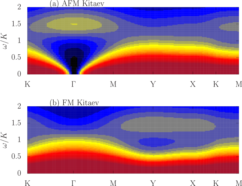
Figure 18: Dynamic structure factor as obtained in Eq. (C), for (a) the AFM Kitaev $K>0$, and (b) the FM Kitaev $K<0$ models. Here we used $\gamma=0.25$, $\Delta=1.05K$ and $g^{2}T=0.1K$.

At finite $g>0$, the infinite series in Eq. (15), becomes a $2\times 2$ matrix equation, with

$$G_{0}(\omega)=\left(\begin{array}[]{cc}-i\omega+\gamma\Delta&\gamma K\\ \gamma K&-i\omega+\gamma\Delta\end{array}\right)^{-1},$$ (34)

while the self energy calculation yields

$$\Sigma(\omega)=-g^{2}K^{2}\frac{1}{-i\omega+2\gamma\Delta}\frac{T}{\Delta^{2}-K^{2}}\left(\begin{array}[]{cc}\Delta&K\\ K&\Delta\end{array}\right).$$ (35)

Using Eq. (15), we obtain

$$C(\omega) \approx \frac{1}{2}\sum_{m=\pm 1}\left(\begin{array}[]{cc}1&m\\ m&1\end{array}\right)$$

$$\quad\quad\times\frac{2\gamma T}{\left|-i\omega+\gamma(\Delta+mK)+\frac{g^{2}K^{2}T}{\Delta^{2}-K^{2}}\frac{\Delta+mK}{-i\omega+2\gamma\Delta}\right|^{2}}.$$

We obtain the dynamic structure factor by Fourier transforming this result, see Fig. 18. Note, for example, that only the $m=1$ term contributes to the dynamic structure factor at ${\bf q}=0$, which is suppressed at low frequencies for the AFM Kitaev, $K>0$. Evidently, the self-energy, Eq. (35), is larger for $m=1$, producing a precession peak at finite $\omega$, where the low frequency correlations are suppressed.

Appendix D Details of the ED calculation

When every eigenvalue $\{E_{\nu}\}$ and eigenvector $\{\ket{\nu}\}$ of the hamiltonian $\mathcal{H}$ are known, the Green’s function at a finite temperature $\beta^{-1}$ is given as

$$\displaystyle\mathcal{G}^{AB}_{\beta}(\omega)=\sum_{\nu,\mu}\frac{e^{-\beta E_{\nu}}}{Z(\beta)}\frac{\bra{\nu}{A}^{\dagger}\ket{\mu}\bra{\mu}{B}^{\ }\ket{\nu}}{\omega+i\eta+E_{\nu}-E_{\mu}},$$ (39)

where $Z$ is the partition function of the system defined as $\displaystyle Z(\beta)=\sum_{\nu}e^{-\beta E_{\nu}}$. For later use, we rewrite the above expression of $\mathcal{G}^{AB}_{\beta}$ as

$$\mathcal{G}^{AB}_{\beta}(\omega)=\displaystyle\sum_{\nu}\frac{e^{-\beta E_{\nu}}}{Z(\beta)}\bra{\nu}{A}^{\dagger}\frac{1}{\omega+i\eta+E_{\nu}-\mathcal{H}}{B}^{\ }\ket{\nu}.$$

Here, we reformulate Eq.(D) with a typical pure state Imada and Takahashi (1986); Skilling (2013); de Vries and De Raedt (1993); Jaklič and Prelovšek (1994); Hams and De Raedt (2000); Sugiura and Shimizu (2012, 2013) $\ket{\psi_{\beta}}$ to avoid using the whole set of $E_{\nu}$ and $\ket{\nu}$. First, we note that the normalized typical state is naively expected to behave as

$$\ket{\psi_{\beta}}\sim\sum_{\nu}e^{i\varphi_{\nu}}\frac{e^{-\frac{\beta}{2}E_{\nu}}}{\sqrt{Z(\beta)}}\ket{\nu},$$ (41)

where $\varphi_{\nu}\in[0,2\pi)$ are random numbers. By introducing a projection operator,

$$\hat{P}_{\nu}=\ket{\nu}\bra{\nu},$$ (42)

we rewrite the formula based on canonical ensemble, Eq.(D), as

$$\mathcal{G}^{AB}_{\beta}(\zeta)\sim\sum_{\nu}\bra{\psi_{\beta}}\hat{P}_{\nu}{A}^{\dagger}\frac{1}{\zeta+E_{\nu}-\mathcal{H}}{B}\hat{P}_{\nu}\ket{\psi_{\beta}}.$$ (43)

Thus far, the exact projection operator $\hat{P}_{\nu}$ requires the whole set of $\ket{\nu}$.

The important step is to find an efficient implementation of the projection operator $\hat{P}_{\nu}$. Although there is no $\mathcal{O}(N_{\rm F})$ implementation of the exact $\hat{P}_{\nu}$ in the literature as far as we know, where $N_{\rm F}$ is the dimension of the Fock space, there is a filter operator Kato (1949); Sakurai and Sugiura (2003); Ikegami et al. (2010); Shimizu et al. (2016) that constructs equi-energy shells and is realizable with the numerical cost of $\mathcal{O}(N_{\rm F})$ by employing the shifted Krylov method Frommer (2003), as follows.

The filter operator Kato (1949) is defined by integrating the resolvent of $\hat{H}$ along a contour $C_{\gamma,\rho}$ defined by $z=\rho e^{i\theta}+\gamma$ with $0\leq\theta<2\pi$ as

$$\hat{P}_{\gamma,\rho}=\frac{1}{2\pi i}\oint_{C_{\gamma,\rho}}\frac{dz}{z-\mathcal{H}}.$$ (44)

If the filter operator is applied to an arbitrary wave function $\ket{\phi}=\sum_{\nu}d_{\nu}\ket{\nu}$, the operator filters the eigenvectors with the eigenvalues $E_{\nu}\not\in(\gamma-\rho,\gamma+\rho)$. When a small $\gamma$ limit is taken, the filter operator realizes a microcanonical ensemble. The filter operator is practically implemented as a Reimann sum Sakurai and Sugiura (2003); Ikegami et al. (2010): The discretized filter operator is defined as

$$\hat{P}_{\gamma,\rho,M}=\frac{1}{M}\sum_{j=1}^{M}\frac{\rho e^{i\theta_{j}}}{\rho e^{i\theta_{j}}+\gamma-\mathcal{H}},$$ (45)

where $\theta_{j}=2\pi(j-1/2)/M$. Multiplication of $\hat{P}_{\gamma,\rho,M}$ to a wave function is simply realized by the shifted Krylov subspace method while it is hardly achievable by the standard Lanczos algorithm.

By introducing an appropriate energy grid measured from the low-energy onset $E_{\rm b}$ in energy axis,

$$\mathcal{E}_{m}=E_{\rm b}+(2m+1)\epsilon,$$ (46)

the set of the filter operators $\{\hat{P}_{\mathcal{E}_{m},\epsilon,M}\}$ with the discretization parameters,

$$\mbox{\boldmath$\delta$}=(E_{\rm b},\epsilon,M),$$ (47)

indeed replace the projection operators $\{\hat{P}_{n}\}$. The filtered typical state given by

$$\ket{\phi_{\beta,\mbox{\boldmath$\delta$}}^{m}}=\hat{P}_{\mathcal{E}_{m},\epsilon,M}\ket{\phi_{\beta}}$$ (48)

is a random vector residing in an equi-energy shell $(\mathcal{E}_{m}-\epsilon,\mathcal{E}_{m}+\epsilon)$, which corresponds to a microcanonical ensemble.

A representation of the Green’s function is thus achieved by employing the filtered typical pure states $\{\ket{\psi_{\beta,\mbox{\boldmath$\delta$}}^{m}}\}$ as

$$\widetilde{\mathcal{G}}_{\beta,\mbox{\boldmath$\delta$}}^{AB}(\zeta)=\sum_{m=0}^{L-1}\bra{\psi_{\beta,\mbox{\boldmath$\delta$}}^{m}}{A}^{\dagger}\frac{1}{\zeta+\mathcal{E}_{m}-\mathcal{H}}{B}\ket{\psi_{\beta,\mbox{\boldmath$\delta$}}^{m}}.$$ (49)

After taking appropriate limits and average over the distribution of the initial random vectors of the typical pure states, we indeed replace the canonical ensemble prescription by the typical pure state formula. By setting $\zeta=\omega+i\eta$ and

$${A}={B}=\hat{S}_{+\mbox{\boldmath$Q$}}^{\alpha}\equiv N^{-1/2}\sum_{\ell}e^{+i\mbox{\boldmath$Q$}\cdot\mbox{\boldmath$R$}_{\ell}}{S}^{\alpha}_{\ell},$$ (50)

in Eq.(49), we obtain the dynamical spin structure factor at a momentum $Q$ and a frequency $\omega$ as,

$$\widetilde{S}_{\beta,\mbox{\boldmath$\delta$}}(\mbox{\boldmath$Q$},\omega) = -\frac{1}{\pi}{\rm Im}\sum_{\alpha=x,y,z}\sum_{m=0}^{L-1}\bra{\psi_{\beta,\mbox{\boldmath$\delta$}}^{m}}{S}^{\alpha}_{-\mbox{\boldmath$Q$}}$$ (51)

$$\times\frac{1}{\omega+i\eta+\mathcal{E}_{m}-\mathcal{H}}{S}^{\alpha}_{+\mbox{\boldmath$Q$}}\ket{\psi_{\beta,\mbox{\boldmath$\delta$}}^{m}},$$

where ${S}_{\ell}^{\alpha}$ ($\alpha=x,y,z$) is an $S$=1/2 spin operator.

In the present paper, we set $E_{\rm b}$ in Eq.(47) as $E_{\rm b}=-8.6$ $(<E_{0}\simeq-8.57)$ for the 24 site cluster of the $\Gamma$ model. The distance among the energy grid points $2\epsilon$ is set as $(E_{\rm cut}-E_{\rm b})/L$, where $L=128$ and $E_{\rm cut}$ is chosen depending on $T$ as $E_{\rm cut}=\max\{\min\{|E_{\rm b}|,T\ln 10^{14}+E_{\rm b}\},4\}$. A random vector is chosen as a typical pure state $|\psi_{0}\rangle$ at infinite temperature. Then, a typical pure state at finite inverse temperature $\beta$ is given by $|\psi_{\beta}\rangle=e^{-\beta\mathcal{H}/2}|\psi_{0}\rangle/\langle\psi_{0}|e^{-\beta\mathcal{H}}|\psi_{0}\rangle$.

Appendix E High temperature expansion

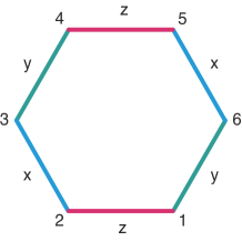
Figure 19: (color online): Site indices used in calculations of spin correlations.

Here, high temperature expansion (small $\beta$ expansion) of static spin correlations is obtained up to third order of $\beta$. Within the language of thermal pure quantum states Sugiura and Shimizu (2013) one can write the finite temperature expectation value of an operator ${O}$ as

$$\langle{O}\rangle=\frac{\displaystyle\mathbb{E}\left[\left(\sum_{\nu}c^{\ast}_{\nu}\bra{\nu}\right)e^{-\beta\mathcal{H}/2}{O}e^{-\beta\mathcal{H}/2}\left(\sum_{\mu}c_{\mu}\ket{\mu}\right)\right]}{\displaystyle\mathbb{E}\left[\left(\sum_{\nu}c^{\ast}_{\nu}\bra{\nu}\right)e^{-\beta\mathcal{H}}\left(\sum_{\mu}c_{\mu}\ket{\mu}\right)\right]},$$

where $\{c_{\nu}\}$ is a set of random complex numbers that satisfy the normalization $\sum_{\nu}|c_{\nu}|^{2}=1$ and the average $\mathbb{E}[\cdots]$ is taken over the probability distribution of the random complex numbers. The denominator is estimated as

$$\mathbb{E}\left[\left(\sum_{\nu}c^{\ast}_{\nu}\bra{\nu}\right)e^{-\beta\mathcal{H}}\left(\sum_{\mu}c_{\mu}\ket{\mu}\right)\right]$$

$$\displaystyle=1+\frac{\beta^{2}}{2N_{\rm F}}{\rm tr}[\mathcal{H}^{2}]+\frac{\beta^{4}}{24N_{\rm F}}{\rm tr}[\mathcal{H}^{4}]+\mathcal{O}(\beta^{6}),$$ (53)

where $N_{\rm F}$ is the Fock space dimension and $\mathbb{E}[c_{\nu}^{\ast}c_{\mu}]=\delta_{\nu,\mu}/N_{\rm F}$ is used. Then, the numerator is estimated by expanding it with respect to $\beta$. The first term is

$$\mathbb{E}\left[\left(\sum_{\nu}c^{\ast}_{\nu}\bra{\nu}\right){O}\left(\sum_{\mu}c_{\mu}\ket{\mu}\right)\right]$$

$$=\sum_{\nu,\mu}\mathbb{E}[c^{\ast}_{\nu}c_{\mu}]\bra{\nu}{O}\ket{\mu}$$

$$=\frac{1}{N_{\rm F}}\sum_{\nu}\bra{\nu}{O}\ket{\nu}=\frac{1}{N_{\rm F}}{\rm tr}[{O}].$$ (54)

The higher order terms are given by

$$({\rm 2nd\ term}) = -\frac{\beta}{2N_{\rm F}}{\rm tr}[{O}\mathcal{H}+\mathcal{H}{O}],$$ (55)

$$({\rm 3rd\ term}) = \frac{\beta^{2}}{4N_{\rm F}}{\rm tr}[\frac{1}{2}{O}\mathcal{H}^{2}+\mathcal{H}{O}\mathcal{H}+\frac{1}{2}\mathcal{H}^{2}{O}],$$ (56)

$$({\rm 4th\ term}) = -\frac{\beta^{3}}{8N_{\rm F}}{\rm tr}[\frac{1}{6}{O}\mathcal{H}^{3}+\frac{1}{2}\mathcal{H}{O}\mathcal{H}^{2}$$ (57)

$$\quad\quad+\frac{1}{2}\mathcal{H}^{2}{O}\mathcal{H}+\frac{1}{6}\mathcal{H}^{3}{O}].$$

When ${O}$ is a spin-spin correlation defined by $\prod_{\ell}\left(S^{x}_{\ell}\right)^{n_{\ell x}}\left(S^{z}_{\ell}\right)^{n_{\ell y}}\left(S^{z}_{\ell}\right)^{n_{\ell z}}$ ($n_{\ell\alpha}=0,1$), ${\rm tr}[{O}]=0$ or, at least, ${\rm tr}[{O}]\ll N_{\rm F}$ for $\sum_{\ell,\alpha}n_{\ell\alpha}\neq 0$, because ${\rm tr}[{O}]/N_{\rm F}$ is the expectation value $\langle{O}\rangle$ at $\beta=0$. Only if ${O}$ is the identity matrix, ${\rm tr}[{O}]=N_{\rm F}$.

E.1 $yx$ correlation for nearest neighbor $z$ bond

The high temperature expansion of $\langle S^{y}_{\mbox{\boldmath$0$}}S^{x}_{\mbox{\boldmath$r$}}\rangle$ for the nearest neighbor $z$ bonds is given as follows. The lowest order of a finite ${\rm tr}[\mathcal{H}^{m}{S}^{y}_{2}{S}^{x}_{1}\mathcal{H}^{n}]/N_{\rm F}$ (see Fig. 19 for the site indices) is given by

$$\Gamma{S}^{y}_{2}{S}^{x}_{1}\cdot{S}^{y}_{2}{S}^{x}_{1}=\frac{\Gamma}{16}.$$ (58)

When we set $O={S}^{y}_{2}{S}^{x}_{1}$ in Eq. (55),

$$({\rm 2nd\ term}) = -\frac{\beta\Gamma}{16}.$$ (59)

E.2 $zz$ correlation for nearest neighbor $z$ bond

The high temperature expansion of $\langle S^{z}_{\mbox{\boldmath$0$}}S^{z}_{\mbox{\boldmath$r$}}\rangle$ for the nearest neighbor $z$ bonds is given as follows. The lowest order of a finite ${\rm tr}[\mathcal{H}^{m}{S}^{z}_{2}{S}^{z}_{1}\mathcal{H}^{n}]/N_{\rm F}$ (see Fig. 19 for the site indices) is, for example, given by

$$\Gamma^{2}{S}^{z}_{2}{S}^{z}_{1}{S}^{x}_{2}{S}^{y}_{1}{S}^{y}_{2}{S}^{x}_{1}=\frac{\Gamma^{2}}{64}.$$ (60)

Then, if we set ${O}={S}^{z}_{2}{S}^{z}_{1}$ in Eqs. (55) and (56),

$$({\rm 2nd\ term}) = 0,$$ (61)

$$({\rm 3rd\ term}) = \frac{\beta^{2}\Gamma^{2}}{64}.$$ (62)

E.3 $zz$ correlation for third nearest neighbor

The high temperature expansion of $\langle S^{z}_{\mbox{\boldmath$0$}}S^{z}_{\mbox{\boldmath$r$}}\rangle$ for the third nearest neighbor pairs across hexagons is given as follows. The lowest order of a finite ${\rm tr}[\mathcal{H}^{m}{S}^{z}_{3}{S}^{z}_{6}\mathcal{H}^{n}]/N_{\rm F}$ (see Fig. 19 for the site indices) is, for example, given by

$$\Gamma^{3}{S}^{z}_{3}{S}^{z}_{6}\cdot{S}^{z}_{3}{S}^{y}_{2}\cdot{S}^{y}_{2}{S}^{x}_{1}\cdot{S}^{z}_{1}{S}^{z}_{6}=\frac{\Gamma^{3}}{256},$$ (63)

or

$$\Gamma^{3}{S}^{z}_{3}{S}^{z}_{6}\cdot{S}^{z}_{3}{S}^{x}_{4}\cdot{S}^{x}_{4}{S}^{y}_{5}\cdot{S}^{y}_{5}{S}^{z}_{6}=\frac{\Gamma^{3}}{256}.$$ (64)

Then, if we set ${O}={S}^{z}_{3}{S}^{z}_{6}$ in Eqs. (55), (56), and (57),

$$({\rm 2nd\ term}) = 0,$$ (65)

$$({\rm 3rd\ term}) = 0,$$ (66)

$$({\rm 4th\ term}) = \frac{3\Gamma^{3}\beta^{3}}{384}.$$ (67)

References

- Kitaev (2006) Alexei Kitaev, “Anyons in an exactly solved model and beyond,” Annals of Physics 321, 2–111 (2006).
- Samarakoon et al. (2017) A. M. Samarakoon, A. Banerjee, S.-S. Zhang, Y. Kamiya, S. E. Nagler, D. A. Tennant, S.-H. Lee, and C. D. Batista, “Comprehensive study of the dynamics of a classical Kitaev spin liquid,” Phys. Rev. B 96, 134408 (2017).
- Knolle et al. (2014) J. Knolle, D. L. Kovrizhin, J. T. Chalker, and R. Moessner, “Dynamics of a Two-Dimensional Quantum Spin Liquid: Signatures of Emergent Majorana Fermions and Fluxes,” Phys. Rev. Lett. 112, 207203 (2014).
- Knolle et al. (2015) J. Knolle, D. L. Kovrizhin, J. T. Chalker, and R. Moessner, “Dynamics of fractionalization in quantum spin liquids,” Phys. Rev. B 92, 115127 (2015).
- Baskaran et al. (2007) G. Baskaran, Saptarshi Mandal, and R. Shankar, “Exact Results for Spin Dynamics and Fractionalization in the Kitaev Model,” Phys. Rev. Lett. 98, 247201 (2007).
- Nasu et al. (2015) Joji Nasu, Masafumi Udagawa, and Yukitoshi Motome, “Thermal fractionalization of quantum spins in a Kitaev model: Temperature-linear specific heat and coherent transport of majorana fermions,” Phys. Rev. B 92, 115122 (2015).
- Rau et al. (2014) Jeffrey G. Rau, Eric Kin-Ho Lee, and Hae-Young Kee, “Generic Spin Model for the Honeycomb Iridates beyond the Kitaev Limit,” Phys. Rev. Lett. 112, 077204 (2014).
- Rousochatzakis and Perkins (2017) Ioannis Rousochatzakis and Natalia B. Perkins, “Classical Spin Liquid Instability Driven By Off-Diagonal Exchange in Strong Spin-Orbit Magnets,” Physical Review Letters 118, 147204 (2017).
- Jackeli and Khaliullin (2009) G. Jackeli and G. Khaliullin, “Mott Insulators in the Strong Spin-Orbit Coupling Limit: From Heisenberg to a Quantum Compass and Kitaev Models,” Phys. Rev. Lett. 102, 017205 (2009).
- Witczak-Krempa et al. (2014) William Witczak-Krempa, Gang Chen, Yong Baek Kim, and Leon Balents, “Correlated Quantum Phenomena in the Strong Spin-Orbit Regime,” Annual Review of Condensed Matter Physics 5, 57–82 (2014).
- Plumb et al. (2014) K. W. Plumb, J. P. Clancy, L. J. Sandilands, V. Vijay Shankar, Y. F. Hu, K. S. Burch, Hae-Young Kee, and Young-June Kim, “-RuCl3: A spin-orbit assisted Mott insulator on a honeycomb lattice,” Physical Review B 90, 041112 (2014).
- Sears et al. (2015) J. A. Sears, M. Songvilay, K. W. Plumb, J. P. Clancy, Y. Qiu, Y. Zhao, D. Parshall, and Young-June Kim, “Magnetic order in -RuCl3: A honeycomb-lattice quantum magnet with strong spin-orbit coupling,” Physical Review B 91, 144420 (2015).
- Johnson et al. (2015) R. D. Johnson, S. C. Williams, A. A. Haghighirad, J. Singleton, V. Zapf, P. Manuel, I. I. Mazin, Y. Li, H. O. Jeschke, R. Valentí, and R. Coldea, “Monoclinic crystal structure of -RuCl3 and the zigzag antiferromagnetic ground state,” Physical Review B 92, 235119 (2015).
- Rau et al. (2016) Jeffrey G. Rau, Eric Kin-Ho Lee, and Hae-Young Kee, “Spin-orbit physics giving rise to novel phases in correlated systems: Iridates and related materials,” Annual Review of Condensed Matter Physics 7, 195–221 (2016).
- Winter et al. (2016) Stephen M. Winter, Ying Li, Harald O. Jeschke, and Roser Valentí, “Challenges in design of Kitaev materials: Magnetic interactions from competing energy scales,” Phys. Rev. B 93, 214431 (2016).
- Winter et al. (2017a) Stephen M. Winter, Alexander A. Tsirlin, Maria Daghofer, Jeroen van den Brink, Yogesh Singh, Philipp Gegenwart, and Roser Valentí, “Models and Materials for Generalized Kitaev Magnetism,” Journal of Physics: Condensed Matter 29, 493002 (2017a).
- Trebst (2017) S. Trebst, “Kitaev Materials,” ArXiv e-prints (2017), arXiv:1701.07056 [cond-mat.str-el] .
- Sears et al. (2017) J. A. Sears, Y. Zhao, Z. Xu, J. W. Lynn, and Young-June Kim, “Phase diagram of -RuCl3 in an in-plane magnetic field,” Physical Review B 95, 180411 (2017).
- Do et al. (2017) Seung-Hwan Do, Sang-Youn Park, Junki Yoshitake, Joji Nasu, Yukitoshi Motome, Yong Seung Kwon, D. T. Adroja, D. J. Voneshen, Kyoo Kim, T.-H. Jang, J.-H. Park, Kwang-Yong Choi, and Sungdae Ji, “Incarnation of Majorana Fermions in Kitaev Quantum Spin Lattice,” arXiv:1703.01081 [cond-mat] (2017), arXiv: 1703.01081.
- Hentrich et al. (2018) Richard Hentrich, Anja U. B. Wolter, Xenophon Zotos, Wolfram Brenig, Domenic Nowak, Anna Isaeva, Thomas Doert, Arnab Banerjee, Paula Lampen-Kelley, David G. Mandrus, Stephen E. Nagler, Jennifer Sears, Young-June Kim, Bernd Büchner, and Christian Hess, “Unusual Phonon Heat Transport in -RuCl3: Strong Spin-Phonon Scattering and Field-Induced Spin Gap,” Phys. Rev. Lett. 120, 117204 (2018).
- Wolter et al. (2017) A. U. B. Wolter, L. T. Corredor, L. Janssen, K. Nenkov, S. Schönecker, S.-H. Do, K.-Y. Choi, R. Albrecht, J. Hunger, T. Doert, M. Vojta, and B. Büchner, “Field-induced quantum criticality in the Kitaev system -RuCl3,” Physical Review B 96, 041405 (2017).
- Winter et al. (2017b) Stephen M. Winter, Kira Riedl, Pavel A. Maksimov, Alexander L. Chernyshev, Andreas Honecker, and Roser Valentí, “Breakdown of magnons in a strongly spin-orbital coupled magnet,” Nature Communications 8, 1152 (2017b).
- Winter et al. (2018) Stephen M. Winter, Kira Riedl, David Kaib, Radu Coldea, and Roser Valentí, “Probing -RuCl3 Beyond Magnetic Order: Effects of Temperature and Magnetic Field,” Physical Review Letters 120, 077203 (2018).
- Catuneanu et al. (2018) Andrei Catuneanu, Youhei Yamaji, Gideon Wachtel, Yong Baek Kim, and Hae-Young Kee, “Path to stable quantum spin liquids in spin-orbit coupled correlated materials,” npj Quantum Materials 3, 23 (2018).
- Gohlke et al. (2018) Matthias Gohlke, Gideon Wachtel, Youhei Yamaji, Frank Pollmann, and Yong Baek Kim, “Quantum spin liquid signatures in Kitaev-like frustrated magnets,” Physical Review B 97, 075126 (2018).
- Conlon and Chalker (2009) P. H. Conlon and J. T. Chalker, “Spin dynamics in pyrochlore heisenberg antiferromagnets,” Phys. Rev. Lett. 102, 237206 (2009).
- Martin et al. (1973) P. C. Martin, E. D. Siggia, and H. A. Rose, “Statistical Dynamics of Classical Systems,” Phys. Rev. A 8, 423–437 (1973).
- De Dominicis and Peliti (1978) C. De Dominicis and L. Peliti, “Field-theory renormalization and critical dynamics above : Helium, antiferromagnets, and liquid-gas systems,” Phys. Rev. B 18, 353–376 (1978).
- Wachtel and Orgad (2014) Gideon Wachtel and Dror Orgad, “Transverse thermoelectric transport in a model of many competing order parameters,” Phys. Rev. B 90, 224506 (2014).
- Hams and De Raedt (2000) Anthony Hams and Hans De Raedt, “Fast algorithm for finding the eigenvalue distribution of very large matrices,” Phys. Rev. E 62, 4365–4377 (2000).
- Sugiura and Shimizu (2013) Sho Sugiura and Akira Shimizu, “Canonical thermal pure quantum state,” Phys. Rev. Lett. 111, 010401 (2013).
- Yamaji et al. (2018) Youhei Yamaji, Takafumi Suzuki, and Mitsuaki Kawamura, “Numerical algorithm for exact finite temperature spectra and its application to frustrated quantum spin systems,” arXiv preprint arXiv:1802.02854 (2018).
- Yamaji et al. (2016) Youhei Yamaji, Takafumi Suzuki, Takuto Yamada, Sei-ichiro Suga, Naoki Kawashima, and Masatoshi Imada, “Clues and criteria for designing a Kitaev spin liquid revealed by thermal and spin excitations of the honeycomb iridate Na2IrO3,” Phys. Rev. B 93, 174425 (2016).
- Banerjee et al. (2016) A. Banerjee, C. A. Bridges, J.-Q. Yan, A. A. Aczel, L. Li, M. B. Stone, G. E. Granroth, M. D. Lumsden, Y. Yiu, J. Knolle, S. Bhattacharjee, D. L. Kovrizhin, R. Moessner, D. A. Tennant, D. G. Mandrus, and S. E. Nagler, “Proximate Kitaev quantum spin liquid behaviour in a honeycomb magnet,” Nat Mater advance online publication (2016), 10.1038/nmat4604.
- Banerjee et al. (2017) Arnab Banerjee, Jiaqiang Yan, Johannes Knolle, Craig A. Bridges, Matthew B. Stone, Mark D. Lumsden, David G. Mandrus, David A. Tennant, Roderich Moessner, and Stephen E. Nagler, “Neutron scattering in the proximate quantum spin liquid -RuCl3,” Science 356, 1055–1059 (2017).
- (36) An ED program package is available through https://github.com/QLMS/HPhi.
- Kawamura et al. (2017) Mitsuaki Kawamura, Kazuyoshi Yoshimi, Takahiro Misawa, Youhei Yamaji, Synge Todo, and Naoki Kawashima, “Quantum lattice model solver ,” Computer Physics Communications 217, 180 – 192 (2017).
- Imada and Takahashi (1986) M. Imada and M. Takahashi, “Quantum transfer Monte Carlo method for finite temperature properties and quantum molecular dynamics method for dynamical correlation functions,” J. Phys. Soc. Jpn. 55, 3354 (1986).
- Skilling (2013) John Skilling, “Maximum entropy and bayesian methods: Cambridge, england, 1988,” (Springer Science & Business Media, 2013) p. 455.
- de Vries and De Raedt (1993) Pedro de Vries and Hans De Raedt, “Solution of the time-dependent Schrödinger equation for two-dimensional spin-1/2 Heisenberg systems,” Phys. Rev. B 47, 7929–7937 (1993).
- Jaklič and Prelovšek (1994) J. Jaklič and P. Prelovšek, “Lanczos method for the calculation of finite-temperature quantities in correlated systems,” Phys. Rev. B 49, 5065–5068 (1994).
- Sugiura and Shimizu (2012) Sho Sugiura and Akira Shimizu, “Thermal pure quantum states at finite temperature,” Phys. Rev. Lett. 108, 240401 (2012).
- Kato (1949) Tosio Kato, “On the convergence of the perturbation method. i,” Progress of Theoretical Physics 4, 514 (1949).
- Sakurai and Sugiura (2003) Tetsuya Sakurai and Hiroshi Sugiura, “A projection method for generalized eigenvalue problems using numerical integration,” Journal of Computational and Applied Mathematics 159, 119 – 128 (2003), 6th Japan-China Joint Seminar on Numerical Mathematics; In Search for the Frontier of Computational and Applied Mathematics toward the 21st Century.
- Ikegami et al. (2010) Tsutomu Ikegami, Tetsuya Sakurai, and Umpei Nagashima, “A filter diagonalization for generalized eigenvalue problems based on the Sakurai–Sugiura projection method,” Journal of Computational and Applied Mathematics 233, 1927–1936 (2010).
- Shimizu et al. (2016) Noritaka Shimizu, Yutaka Utsuno, Yasunori Futamura, Tetsuya Sakurai, Takahiro Mizusaki, and Takaharu Otsuka, “Stochastic estimation of nuclear level density in the nuclear shell model: An application to parity-dependent level density in 58Ni,” Physics Letters B 753, 13 – 17 (2016).
- Frommer (2003) Andreas Frommer, “BiCGstab () for families of shifted linear systems,” Computing 70, 87–109 (2003).