Precision constraints on radiative neutrino decay with CMB spectral distortion

Abstract

We investigate the radiative decay of the cosmic neutrino background, and its impact on the spectrum of the cosmic microwave background (CMB) that is known to be a nearly perfect black body. We derive exact formulae for the decay of a heavier neutrino into a lighter neutrino and a photon, $\nu_{j}\to\nu_{i}+\gamma$, and of absorption as its inverse, $\nu_{i}+\gamma\to\nu_{j}$, by accounting for the precise form of the neutrino momentum distribution. Our calculations show that if the neutrinos are heavier than $\mathcal{O}(0.1)$ eV, the exact formulae give results that differ by $\sim$50%, compared with approximate ones where neutrinos are assumed to be at rest. We also find that spectral distortion due to absorption is more important for heavy neutrino masses (by a factor of $\sim$10 going from a neutrino mass of 0.01 eV to 0.1 eV). By analyzing the CMB spectral data measured with COBE-FIRAS, we obtain lower limits on the neutrino lifetime of $\tau_{12}\gtrsim 4\times 10^{21}$ s (95% C.L.) for the smaller mass splitting and $\tau_{13}\sim\tau_{23}\gtrsim 10^{19}$ s for the larger mass splitting. These represent up to one order of magnitude improvement over previous CMB constraints. With future CMB experiments such as PIXIE, these limits will improve by roughly 4 orders of magnitude. This translates to a projected upper limit on the neutrino magnetic moment (for certain neutrino masses and decay modes) of $\mu_{\nu}<3\times 10^{-11}\,\mu_{B}$, where $\mu_{B}$ is the Bohr magneton. Such constraints would make future precision CMB measurements competitive with lab-based constraints on neutrino magnetic moments.

I Introduction

In the last few decades, many experiments have demonstrated that neutrinos show properties beyond the Standard Model of particle physics. They have nonzero masses and show flavor mixings as revealed by measurements of neutrino oscillations using solar, atmospheric, reactor, and accelerator neutrinos (see Refs. Patrignani et al. (2016); Giganti et al. (2018) for a review). There are, however, a number of important issues remaining: What is the neutrino mass hierarchy Qian and Vogel (2015)? What is the CP violating phase in the lepton sector Hagedorn et al. (2017)? How weakly do neutrinos interact with photons Levine (1967); Cung and Yoshimura (1975)? Do neutrinos decay, either radiatively or non-radiatively Pal and Wolfenstein (1982)?

Even the weak interaction predicts interactions between the neutrino and photon through a non-zero magnetic moment induced via loop corrections of gauge boson, although its value is expected to be small Cung and Yoshimura (1975). We denote by $\mu_{ij}$ the magnetic moment between neutrino mass eigenstates $i$ and $j$, with off-diagonal elements $(i\neq j)$ representing the transition magnetic moments in radiative decay. For massive Dirac neutrinos, the value of the diagonal magnetic moment induced by loops of gauge bosons is given by Fujikawa and Shrock (1980)

$$\mu^{D}_{ii}=\frac{3eG_{F}m_{i}}{8\sqrt{2}\pi^{2}}\approx 3.2\times 10^{-19}\left(\frac{m_{i}}{\mathrm{eV}}\right)\,\mu_{B},$$ (1)

where $\mu_{B}$ is the Bohr magneton, while for the Dirac off-diagonal elements one finds a value roughly $10^{-4}$ times smaller Glashow et al. (1970). For Majorana neutrinos, one finds the magnetic moment suppressed by the ratio of the lepton and gauge boson masses:

$$\mu^{M}_{ij}=\frac{3eG_{F}m_{i}}{16\sqrt{2}\pi^{2}}\left(1+\frac{m_{j}}{m_{i}}\right)\sum_{l=e,\mu,\tau}{\rm Im}\left[U_{lk}U_{lj}^{*}\right]\left(\frac{m_{l}}{m_{W}}\right)^{2}\,.$$ (2)

The current upper bound on the neutrino magnetic moment from electron-neutrino scattering experiments is $\mu_{\nu}<2.8\times 10^{-11}\mu_{B}$ Beda et al. (2013); Agostini et al. (2017a). The strongest astrophysical constraints place the bound at $\mu_{\nu}<2.2\times 10^{-12}\mu_{B}$ Raffelt (1990, 1999); Arceo-Díaz et al. (2015), well above the value expected from weak interactions alone (see Refs. Studenikin (2016, 2018) for a thorough review). However, new physics contributions could enhance the predicted magnetic moment Shrock (1974); Lee and Shrock (1977); Shrock (1982); Georgi and Randall (1990); Davidson et al. (2005); Bell et al. (2005, 2006); Frère et al. (2015). In particular, Ref. Lindner et al. (2017) proposed a model with SU(2) horizontal symmetry, allowing Majorana transition neutrino magnetic moments of order $10^{-12}\,\mu_{B}$ while protecting the small mass of the neutrinos.

Since the neutrinos have masses that are proven to differ for different mass eigenstates, nonzero magnetic moments will induce radiative neutrino decay,

$$\nu_{j}\to\nu_{i}+\gamma,$$ (3)

where $m_{j}>m_{i}$. With enhanced magnetic moments, radiative neutrino decays induced by this interaction may be relevant for astrophysical systems, providing a probe of new physics in the neutrino sector. Since the mass squared differences have been precisely measured with oscillation experiments and the absolute neutrino masses have been constrained to be below $\mathcal{O}(1)$ eV Ade et al. (2016); Gando et al. (2016), Ref. Mirizzi et al. (2007) pointed out that photons emitted via neutrino decay will disturb the nearly perfect black-body spectrum of the cosmic microwave background (CMB). By comparing with the CMB spectral data obtained with the Far Infrared Absolute Spectrophotometer (FIRAS) onboard the Cosmic Background Explorer (COBE) Fixsen et al. (1996); Fixsen and Mather (2002), Ref. Mirizzi et al. (2007) obtained constraints on decay rate as $\Gamma<2\times 10^{-19}$–$5\times 10^{-20}$ s^-1. This corresponds to $\mu_{\nu}\lesssim 10^{-8}\mu_{B}$, still much weaker than other astrophysical or lab-based constraints.

In this paper, we improve the work of Ref. Mirizzi et al. (2007) in several aspects. First, we argue that, if the neutrino can decay radiatively ($\nu_{j}\to\nu_{i}+\gamma$), then it is also possible that a CMB photon is absorbed by a lighter mass eigenstate of the cosmic neutrino background $\nu_{i}$:

$$\nu_{i}+\gamma_{\rm CMB}\to\nu_{j},$$ (4)

to create a heavier state $\nu_{j}$. The cross section of this resonance process is given by

$$\sigma(E)=\frac{\pi^{2}}{k^{2}}\Gamma\delta(E-m_{j}),$$ (5)

where $E$ is the center-of-mass energy of the initial state, and $k$ is the momentum of the center-of-mass frame Patrignani et al. (2016).

Second, in contrast to approximate formulae that were derived and adopted in the literature Masso and Toldra (1999); Mirizzi et al. (2007), where neutrinos were assumed to be at rest, we derive exact formulae by taking the neutrinos’ thermal momentum distribution into account. We also include the effects of stimulated emissions for decay and Pauli blocking for both the decay and absorption. We show that all these effects can be of considerable importance in calculating the CMB spectral distortion. Therefore, neglecting these will cause a theoretical bias in the estimated lower limits on the decay lifetime.

Third, we will make projections for planned future CMB experiments. We will primarily focus on the Primordial Inflation Explorer (PIXIE) Kogut et al. (2011a), which is a proposed mission to measure the CMB intensity with a higher sensitivity and wider frequency range than COBE-FIRAS. PIXIE is expected to have a sensitivity of 5 Jy/sr Chluba and Jeong (2014), as opposed to the COBE-FIRAS sensitivity, which is of the order of $10^{4}$ Jy/sr Fixsen et al. (1996). We show how this improved sensitivity affects constraints on the neutrino lifetime and magnetic moment. We thus motivate future CMB experiments such as PIXIE (and the further-future PRISM experiment Andre et al. (2013)), as probes of New Physics in the neutrino sector. Finally, we note that, when obtaining the current FIRAS bounds and PIXIE sensitivities, we take into account correlations between different components of the spectral distortion such as the chemical potential as well as the residual Galactic emission.

The paper is organized as follows. In Sec. II, we present formulae for computing the intensities of microwave photons from both decay and absorption by cosmic neutrinos. The theoretical results are then compared with the CMB spectral data measured with COBE-FIRAS, and we calculate the lower limits on the decay lifetime and the upper limits on the neutrino magnetic moments for various modes and the different mass hierarchy scenarios in Sec. III. We then discuss the potential sensitivity of future CMB experiments to the neutrino radiative decay in Sec. IV and conclude the paper in Sec. V.

II Decay and absorption intensities

In Sec. II.1, we first derive formulae for photon intensities from both the decay of heavier neutrinos and absorption of the CMB photons by the lighter neutrinos, by assuming that the neutrinos are at rest — a reasonable approximation when the neutrino mass is much larger than the temperature of the CMB and neutrino background, on the order of $10^{-3}$ eV. In Sec. II.2, we show exact formulae for the decay and absorption intensities although much of the derivation is later summarized in Appendix A. In Sec. II.3, we show numerical results for decay and absorption intensities, illustrating their dependence on the lightest neutrino mass, decay mode, and mass hierarchy.

II.1 Approximate formulation

If the neutrino can be considered at rest, according to kinematics, the energy of the absorbed CMB photon $\epsilon_{\gamma}$ (in the observer frame) is related to the neutrino masses via

$$(1+z_{a})\epsilon_{\gamma}=\frac{\Delta m_{ij}^{2}}{2m_{i}},$$ (6)

where we have defined $m_{i}<m_{j}$, $\Delta m_{ij}^{2}\equiv m_{j}^{2}-m_{i}^{2}$, and $z_{a}$ is the redshift when absorption occurs. In contrast, radiative decay follows slightly different kinematics:

$$(1+z_{d})\epsilon_{\gamma}=\frac{\Delta m_{ij}^{2}}{2m_{j}},$$ (7)

with redshift $z_{d}$ when the decay occurs. Setting $z_{a,d}=0$ gives the maximum photon energy at which the effects of absorption or decay can be observed for given $m_{i}$, $m_{j}$.

Equation (5) shows the absorption cross section in terms of quantities in the center-of-mass frame. It is, however, more useful to use quantities in the observer frame where the lighter neutrino $\nu_{i}$ is at rest and $\epsilon_{\gamma}$ is in the microwave frequency range. Then, Eq. (5) can be rewritten as

$$\sigma([1+z]\epsilon_{\gamma}) = \frac{\pi^{2}}{k^{2}}\Gamma\frac{m_{j}}{m_{i}}\delta\left((1+z)\epsilon_{\gamma}-\frac{\Delta m_{ij}^{2}}{2m_{i}}\right)\,.$$ (8)

The center-of-mass momentum $k$ for the absorption, $\nu_{i}+\gamma\to\nu_{j}$, satisfies

$$\sqrt{k^{2}+m_{i}^{2}}+k=m_{j}\,,$$ (9)

according to energy conservation. From this, we have

$$k=\frac{\Delta m_{\ij}^{2}}{2m_{j}}\,,$$ (10)

and thus

$$\sigma([1+z]\epsilon_{\gamma}) = \frac{4\pi^{2}m_{j}^{3}\Gamma}{(\Delta m_{ij}^{2})^{2}m_{i}\epsilon_{\gamma}}\delta(z-z_{a})\,.$$ (11)

We then consider the effective CMB intensity due to decay and absorption, $I_{\rm dec}$ and $I_{\rm abs}$ as a function of CMB energy $\epsilon_{\gamma}$. For a given energy $\epsilon_{\gamma}$, there is a corresponding redshift through Eqs. (6) and (7), where absorption and decay is allowed, respectively. These intensities can be written as a cosmological line-of-sight integral of the emissivity Peacock (1999):

$$I_{\rm dec}(\epsilon_{\gamma}) = \frac{1}{4\pi}\int dz\frac{P_{\rm dec}([1+z]\epsilon_{\gamma},z)}{H(z)(1+z)^{4}}\,,$$ (12)

$$I_{\rm abs}(\epsilon_{\gamma}) = \frac{1}{4\pi}\int dz\frac{P_{\rm abs}([1+z]\epsilon_{\gamma},z)}{H(z)(1+z)^{4}}\,,$$ (13)

where $P_{\rm dec}$ or $P_{\rm abs}$ is the volume emissivity (energy of photons emitted per unit volume, per unit time, and per unit energy range), $H(z)=H_{0}\sqrt{\Omega_{m}(1+z)^{3}+\Omega_{\Lambda}}$, $H_{0}=67.8$ km s^-1 Mpc^-1 is the Hubble constant, $\Omega_{m}=0.308$, and $\Omega_{\Lambda}=0.692$ Ade et al. (2016).

These emissivity functions can therefore be written as

$$P_{\rm dec}([1+z]\epsilon_{\gamma},z) = (1+z)\epsilon_{\gamma}n_{\nu_{j}}(z)\Gamma e^{-\Gamma t(z)}$$ (14)

$${}\times\left[1+f_{\rm CMB}(\epsilon_{\gamma})\right]$$

$${}\times\delta\left((1+z)\epsilon_{\gamma}-\frac{\Delta m_{ij}^{2}}{2m_{j}}\right)$$

$$= (1+z)n_{\nu_{j}}(z)\Gamma e^{-\Gamma t(z)}$$

$${}\times\left[1+f_{\rm CMB}(\epsilon_{\gamma})\right]\delta(z-z_{d}),$$

$$P_{\rm abs}([1+z]\epsilon_{\gamma},z) = -(1+z)\epsilon_{\gamma}n_{\nu_{i}}(z)$$ (15)

$${}\times n_{\rm CMB}([1+z]\epsilon_{\gamma},z)\sigma([1+z]\epsilon_{\gamma})$$

$$= -\frac{2\pi^{2}m_{j}^{3}\Gamma}{\Delta m_{ij}^{2}m_{i}^{2}\epsilon_{\gamma}}\delta(z-z_{a})$$

$${}\times n_{\nu_{i}}(z)n_{\rm CMB}([1+z]\epsilon_{\gamma},z),$$

where note that the sign of $P_{\rm abs}$ is negative as it gives suppression of the total CMB intensity. The term $\left[1+f_{\rm CMB}(\epsilon_{\gamma})\right]$ represents the stimulated emission, with $f_{\rm CMB}(\epsilon_{\gamma})=(e^{{\epsilon_{\gamma}}/T_{\rm CMB}}-1)^{-1}$ the occupation number of the CMB photons and $T_{\rm CMB}=2.725$ K the present CMB temperature Fixsen et al. (1996); Fixsen and Mather (2002), and $n_{\rm CMB}(\epsilon_{\gamma},z)$ is the CMB number density per unit energy range at $\epsilon_{\gamma}$ and $z$: i.e., $n_{\rm CMB}([1+z]\epsilon_{\gamma},z)=(1+z)^{2}\epsilon_{\gamma}^{2}f_{\rm CMB}(\epsilon_{\gamma})/\pi^{2}$. The occupation number has no dependence on redshift, as it cancels between the energy at $z$, $(1+z)\epsilon_{\gamma}$, and the CMB temperature at $z$, $(1+z)T_{\rm CMB}$. We note that the effect of stimulated emission has not been taken into account in the literature Mirizzi et al. (2007); Masso and Toldra (1999), although it was acknowledged in Ref. Masso and Toldra (1999). We also assume $\Gamma t(z)\ll 1$ in the following discussions, which is well justified when the lifetime $\tau=\Gamma^{-1}$ is much larger than the age of the Universe as is the case here. By using Eqs. (14) and (15) in Eqs. (12) and (13) respectively, one can predict the effect of decay and absorption on the CMB intensity spectrum. After the $\delta$-functions collapse the redshift integral, we obtain the following analytic expressions:

$$I_{\rm dec}(\epsilon_{\gamma}) = \frac{1}{4\pi}\frac{n_{\nu_{j}}\Gamma}{H(z_{d})}\left[1+f_{\rm CMB}(\epsilon_{\gamma})\right],$$ (16)

$$I_{\rm abs}(\epsilon_{\gamma}) = -\frac{1}{4\pi}\frac{n_{\nu_{i}}\Gamma}{H(z_{a})}\left(\frac{m_{j}}{m_{i}}\right)^{3}f_{\rm CMB}(\epsilon_{\gamma}),$$ (17)

where $n_{\nu_{i}}=n_{\nu_{j}}\approx 110$ cm^-3 are the neutrino number density of mass eigenstates $\nu_{i}$ and $\nu_{j}$ at $z=0$. Up to the factor for stimulated emission, Eq. (16) agrees with the formulae adopted in Ref. Mirizzi et al. (2007).

II.2 Exact formulation

Thus far, we made the approximation that both $\nu_{i}$ and $\nu_{j}$ in the initial states are at rest. This is a very good approximation when the neutrino can be regarded as nonrelativistic, which is valid in the case of $m_{i,j}\gg T_{\nu}=(4/11)^{1/3}T_{\rm CMB}=1.95$ K. Otherwise, one has to take into account the momentum distribution of the neutrinos Wong (2011):

$$f_{\nu}(p_{\nu},z)=\frac{1}{\exp[p_{\nu}/T_{\nu}(z)]+1},$$ (18)

where $T_{\nu}(z)=(1+z)T_{\nu}$ is the neutrino temperature at $z$.

A detailed derivation of the emissivity is summarized in Appendix A, and here we show only the results:

$$P_{\rm dec}([1+z]\epsilon_{\gamma},z) = \frac{\Gamma T_{\nu}m_{j}\Delta m_{ij}^{2}}{4\pi^{2}}\frac{1+f_{\rm CMB}(\epsilon_{\gamma})}{\epsilon_{\gamma}}U\left(\frac{m_{j}}{(1+z)T_{\nu}},\frac{\epsilon_{\gamma}}{T_{\nu}},\frac{2(1+z)\epsilon_{\gamma}m_{j}}{\Delta m_{ij}^{2}}\right),$$ (19)

$$P_{\rm abs}([1+z]\epsilon_{\gamma},z) = -\frac{2(1+z)^{4}}{\pi^{2}}\frac{\Gamma T_{\nu}^{2}m_{j}^{3}}{(\Delta m_{ij}^{2})^{2}}\epsilon_{\gamma}^{2}f_{\rm CMB}(\epsilon_{\gamma})V\left(\frac{m_{i}}{(1+z)T_{\nu}},\frac{\epsilon_{\gamma}}{T_{\nu}},\frac{2(1+z)\epsilon_{\gamma}m_{i}}{\Delta m_{ij}^{2}}\right),$$ (20)

for decay ($\nu_{j}\to\nu_{i}+\gamma$) and absorption ($\nu_{i}+\gamma\to\nu_{j}$) respectively, where

$$U(y,s,t) = \int_{\frac{y}{2}\left|t-\frac{1}{t}\right|}^{\infty}\frac{dxx}{(e^{x}+1)\sqrt{x^{2}+y^{2}}}$$ (21)

$${}\times\left[1-\frac{1}{e^{W_{-}(s,t,x,y)}+1}\right],$$

$$V(y,s,t) = \int_{\frac{y}{2}\left|t-\frac{1}{t}\right|}^{\infty}\frac{dxx}{e^{x}+1}\left[1-\frac{1}{e^{W_{+}(s,t,x,y)}+1}\right],$$

$$W_{\pm}(s,t,x,y) = \left[s^{2}+x^{2}\pm 2s\left(\sqrt{x^{2}+y^{2}}-\frac{y}{t}\right)\right]^{1/2}.$$

These equations are inevitably more complicated than those shown in the previous subsection, but the most accurate.

II.3 Results

We present numerical results for the intensity due to absorption and decay, as well as comparing the approximate and exact calculations. Because it is not yet known whether the neutrino mass eigenstates are arranged in a normal hierarchy (NH, $m_{1}<m_{2}\ll m_{3}$) or an inverted hierarchy (IH, $m_{3}\ll m_{1}<m_{2}$) we include both possibilities in the calculations presented later in the paper. Throughout the paper, we adopt $\Delta m_{12}^{2}=7.53\times 10^{-5}$ eV² and $\Delta m_{23}^{2}=2.5\times 10^{-3}$ eV² for NH, and $\Delta m_{12}^{2}=7.53\times 10^{-5}$ eV² and $\Delta m_{31}^{2}=2.5\times 10^{-3}$ eV² for IH Patrignani et al. (2016). We show only results for the NH in this section, noting that the results for IH are similar. The mass of the lightest neutrino mass eigenstate is $m_{1}$, and we assume a reference value of $\tau=10^{18}$ s for the neutrino radiative decay lifetime.

Figure 1 shows the effect of decay and absorption on the CMB spectrum, in the case of transitions between $m_{1}$ and $m_{2}$, computed with the approximate formulae. We note first that the distortions to the CMB spectrum extend up to higher frequencies for lighter neutrinos, which is simply a consequence of kinematics [cf. Eqs. (7) and (6)]. We also note that the magnitude of the absorption depends on the masses of the neutrinos, with heavier neutrinos leading to a larger absorption effect. For a given photon energy today $\epsilon_{\gamma}$, as we decrease the mass $m_{i}$ of the absorbing neutrino, the absorption must occur at earlier times (larger redshift, $z_{a}$). As we increase $z_{a}$, the period over which absorption can take place $\sim$$H(z_{a})^{-1}$ becomes shorter, suppressing the total amount of absorptions. Decreasing $m_{i}$ from 0.1 to 0.03 eV, this factor dominates over the $(m_{j}/m_{i})^{3}$ scaling in the absorption intensity [Eq. (17)] and the absorption effect becomes smaller (left panel of Fig. 1).

Decreasing the lightest neutrino mass $m_{i}$ further, one would expect eventually that the $(m_{j}/m_{i})^{3}$ scaling would dominate over the scaling with $\sim$$H(z_{a})^{-1}$$\sim$$(m_{i}/\Delta m_{ij}^{2})^{3/2}$, for high $z$. However, at high $z$ the neutrino temperature is large and the neutrino momenta, described in Eq. 18 become relevant. The non-zero neutrino momenta act to suppress the absorption cross section [Eq. 5] which scales as $k^{2}$, where $k$ is the centre-of-mass from momentum. As we will see in Sec. III, the overall effect is that the absorption intensity flattens to a constant at small values of $m_{i}$. This emphasises the importance of the exact formulation – accounting for the thermal neutrino distribution – for the correct calculation of the absorption effect.

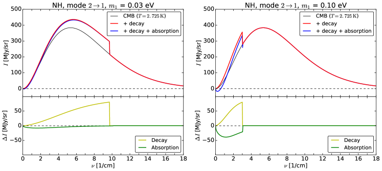
Figure 1: Effect of neutrino decay and photon absorption on the CMB spectrum. Both panels consider NH and $\Gamma=10^{-18}$ s^-1 with decay/absorption between the lowest two mass eigenstates, where the lowest mass is taken to be $0.03$ eV (left) and $0.1$ eV (right). The black lines correspond to the unperturbed CMB spectrum, the red lines include the effect of photons from decaying neutrinos, while the blue lines include both decay and absorption. Here, the intensities as a function of frequency $\nu$ are calculated using the approximate formulae given in Sec. II.1. In the lower panel, the CMB spectrum is not included, and only the bare intensities from decay (yellow) and absorption (green) are shown.

Figures 2 and 3 compare the results of using the exact (green) and approximate (red) calculations for different neutrino masses. In each case, the left panels correspond to the decay/absorption of $m_{1}$ and $m_{2}$, while the right panels show the same for $m_{1}$ and $m_{3}$. Because $\Delta m_{13}^{2}$ is two orders of magnitude larger than $\Delta m_{12}^{2}$, the spectral distortions for the $3\to 1$ mode extend up to much larger photon energies. From Fig. 2, we see the effect of the neutrino momentum distribution, which leads to a smoother cut-off in the intensity when exact formulae are used, compared to the sharp cutoff in approximate approach. Furthermore, at low frequencies, corresponding to high absorption redshift, the approximate absorption intensity is much larger than the exact absorption intensity. This suppression of the absorption intensity is a manifestation of the non-zero neutrino temperature, as described in the previous paragraph. Though these appear to be minor corrections, the high precision of the CMB spectral measurements means that these should be taken into account to obtain accurate limits on the neutrino lifetime.

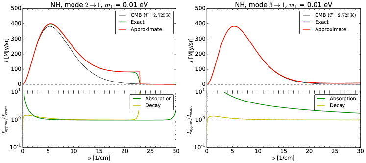
Figure 2: Comparison between the exact and approximate neutrino decay and absorption intensities. The exact results are shown in green and the approximate results in red, as functions of frequency $\nu$. Both left and right-hand panels use a mass of $0.01$ eV for the lightest neutrino, but they consider different modes: $m_{2}\leftrightarrow m_{1}$ (left) and $m_{3}\leftrightarrow m_{1}$ (right). The lower panels show the ratio of the approximate and exact intensities for both absorption and decay.

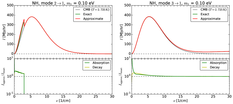
Figure 3: The same as Fig. 2 but for a heavier neutrino mass, $m_{1}=0.1$ eV.

Another effect which is observed in Figs. 2 and 3 is the impact of Pauli blocking. In the exact formalism [Eqs. (19) and (20)], the term $1-1/[e^{W_{\pm}(s,t,x,y)}+1]$, leads to a suppression of the decay and absorption rates when the final neutrino state is already occupied. This Pauli-blocking effect lowers the overall intensity; we see from the lower panels of Figs. 2 and 3 that the approximate intensity is always larger than the exact one, by around 50%. The stimulated emission, on the other hand, enhances the decay intensity, but the effect quickly decreases from $\sim$50% at 2 cm^-1 (the lowest frequency of the FIRAS measurement) to $\lesssim 3$% at $>6$ cm^-1. Therefore, the absorption and Pauli-blocking combined should give lower intensities than were found with the formulae used in Ref. Mirizzi et al. (2007).

III Analysis of the COBE-FIRAS data of CMB spectrum and lower limits on decay lifetime

III.1 Maximum likelihood analysis

COBE-FIRAS has precisely measured the CMB spectrum, in order to constrain cosmological parameters Fixsen et al. (1996). The model for the CMB intensity discussed there included the effects of temperature deviations, Galactic contamination, chemical potential $\mu$, and $y$-distortion. Since we also include the decay and absorption, we consider an intensity $I$ of the form

$$I = I_{0}+\Delta T\frac{\partial I_{\nu}}{\partial T}+\mu\frac{\partial I_{\nu}}{\partial\mu}+G_{0}I_{gal}+yI_{y}$$ (24)

$${}+\Gamma_{ij}\left(I_{ij}^{\rm dec}+I_{ij}^{\rm abs}\right),$$

where the derivatives are to be evaluated at $T=T_{0}=2.725$ K and $\mu=0$, and $\Delta T\equiv T-T_{0}$. The index $ij$ denotes the decay/absorption mode between the different mass eigenstates of the neutrino: $ij\in\{12,13,23\}$. Furthermore $G_{0}$ is the amplitude of the Galactic contamination, $y$ is the Kompaneets $y$ parameter, and $\Gamma_{ij}$ is the decay rate for mode $ij$. $I_{0}$ is a regular black-body spectrum:

$$I_{0}=I_{\nu}(T,\mu)\big{\rvert}_{T=T_{0},\mu=0}=\frac{2h\nu^{3}}{e^{h\nu/T+\mu}-1}\bigg{\rvert}_{T=T_{0},\mu=0},$$ (25)

$I_{gal}$ is the residual Galactic contamination measured by FIRAS, $I_{y}$ is given by Zeldovich and Sunyaev (1969); Fixsen et al. (1996)

$$I_{y}=T_{0}\left[\frac{h\nu}{T_{0}}\coth\left(\frac{1}{2}\frac{h\nu}{T_{0}}\right)-4\right]\frac{\partial I_{\nu}}{\partial T}\bigg{\rvert}_{T=T_{0},\mu=0},$$ (26)

and $I_{ij}^{\rm dec}$, $I_{ij}^{\rm abs}$ are intensities corresponding to decay and absorption, respectively, of mode $ij$ per unit $\Gamma$. Note that in reality, all three modes occur simultaneously, but we find that including them all at once in the analysis would yield unnecessarily weak constraints on $\Gamma_{ij}$. This is because the masses of $\nu_{1}$ and $\nu_{2}$ are relatively close, resulting in degeneracy in the spectra of the modes 13 and 23. We solve this issue by focusing on one mode at a time, forcing the other two decay rates to be zero.

The parameters we are interested in are $\Gamma_{12}$, $\Gamma_{13}$ and $\Gamma_{23}$. We will constrain these by fitting the model in Eq. (24) to the FIRAS data, and minimizing $\chi^{2}$ as a function of the parameters $\Delta T$, $\mu$, $G_{0}$, $y$, and $\Gamma_{ij}$. The $\chi^{2}$ of this model is given by

$$\chi^{2}=\sum_{i,j=1}^{43}(I^{\rm data}_{i}-I^{\rm model}_{i})(C^{-1})_{ij}(I^{\rm data}_{j}-I^{\rm model}_{j}),$$ (27)

where $I^{\rm model}$ is given by Eq. (24), $I^{\rm data}$ is the FIRAS measurement, and $C$ is the covariance matrix taken from Ref. Fixsen et al. (1996). The sum runs over the 43 frequency bins of FIRAS.

Our model for the intensity is defined by the parameters $\theta_{a}\in\{\Delta T,\mu,G_{0},y,\Gamma_{ij}\}$, whose best fit values $\hat{\theta}_{a}$ are determined by solving the system of 5 simultaneous equations:

$$\left.\frac{\partial\chi^{2}}{\partial\theta_{a}}\right|_{{\hat{\bm{\theta}}}}=0.$$ (28)

In order to estimate errors for each parameter $\theta_{a}$, taking degeneracy among the parameters into account, we calculate the Observed Fisher Information matrix:

$$F_{ab}=\frac{1}{2}\frac{\partial^{2}\chi^{2}}{\partial\theta_{a}\partial\theta_{b}}.$$ (29)

The parameters $\theta_{a},\,\theta_{b}\in\{\Delta T,\mu,G_{0},y,\Gamma_{ij}\}$ so $\dim(F)=5$, since we are only looking at one decay mode at a time. The derivatives in Eq. (29) are to be evaluated at the best-fit point $\hat{\theta}_{a}$. However, we note that assuming the linearized intensity in Eq. (24), the Fisher Information is independent of the parameters $\theta_{a}$ and $\theta_{b}$.

The covariance between parameters $\theta_{a}$ and $\theta_{b}$ is the inverse of this matrix:

$$\mbox{Cov}(\theta_{a},\theta_{b})=\left(F^{-1}\right)_{ab}\,.$$ (30)

The $1\sigma$ uncertainty of a specific parameter $\theta_{a}$ is equivalent to the diagonal components of the covariance matrix as follows:

$$\sigma_{a}=\sqrt{\left(F^{-1}\right)_{aa}}\,.$$ (31)

The upper limit at 95% confidence level (C.L.) on the parameter $\theta_{a}$ (corresponding to $\Delta\chi^{2}\approx 2.71$) is then estimated as

$$\theta_{a}^{95\%}\approx\hat{\theta}_{a}+\sqrt{2.71}\,\sigma_{a}\,.$$ (32)

In some cases, we find that the best-fit value, $\hat{\Gamma}$, is negative, which is clearly unphysical. In this case, we assume that Eq. (29) remains a good approximation to the $\chi^{2}$. The physical best-fit is then at $\Gamma=0$ and we calculate the upper limit as:

$$\Gamma^{95\%}\approx\hat{\Gamma}+\sqrt{\hat{\Gamma}^{2}+2.71\,\sigma_{\Gamma}^{2}}\,.$$ (33)

We have checked our analysis procedure by fixing $\Gamma=0$ and determining limits on the $\mu$ and $y$ paramater separately. Our results are consistent with those reported in Ref. Fixsen et al. (1996) ($|\mu|<9\times 10^{-5}$ and $|y|<1.5\times 10^{-5}$ at 95% CL).

III.2 Constraints on neutrino decay lifetime and transition magnetic moments

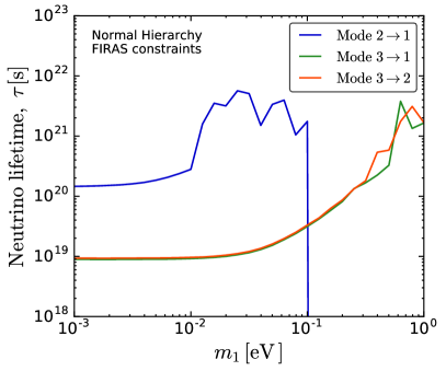
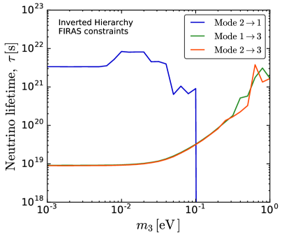
Figure 4: 95% C.L. lower limits on radiative decay lifetime of neutrinos as a function of the lightest neutrino mass. Values of the neutrino lifetime below the solid curves are excluded by our analysis at the 95% C.L. Left panel: Results for NH, where $m_{1}$ is the lowest mass. Right panel: Results for IH where $m_{3}$ is the lowest mass.

Using the approach given in the previous subsection, and the FIRAS data Fixsen et al. (1996), we numerically compute values for the 95% C.L. lower limit on the neutrino lifetime $\tau=1/\Gamma$ as a function of the lowest neutrino mass. These constraints are presented in Fig. 4 for NH (left panel) and IH (right panel).

Constraints on the 13 and 23 modes are weaker than for the 12 mode by around an order of magnitude. This is as expected comparing, e.g., the left and right panels of Fig. 2, where the distortion due to the 12 mode is clearly larger for a fixed value of $\tau$. As outlined in Sec. II.3, this is because the larger mass squared difference in the 13 case means that the majority of the distortion appears at frequencies above the FIRAS range. For the 12 mode, the strongest constraints appear in the mass range 0.01–0.12 eV, below which the sharp spectral feature from neutrino decay lies above the FIRAS frequency range. Above $\sim$0.12 eV, the CMB distortions from neutrino decay and absorption occur at too low frequencies to be detected by FIRAS. As pointed out in Ref. Mirizzi et al. (2007), the jagged shape of the limits is due to the fact that the $\chi^{2}$ changes abruptly when the end-point of the neutrino decay spectrum crosses into a new frequency bin.

We now translate our constraints on the radiative neutrino decay rate $\Gamma$ into constraints on the effective neutrino magnetic moment. For neutrinos with transition magnetic and electric moments, $\mu_{ij}$ and $\epsilon_{ij}$, respectively, we can define the effective magnetic moment $\kappa_{ij}^{2}\equiv|\mu_{ij}|^{2}+|\epsilon_{ij}|^{2}$. For a transition $\nu_{j}\rightarrow\nu_{i}+\gamma$, the decay rate induced by this magnetic moment is given by Raffelt (1996):

$$\Gamma_{ij}=\frac{\kappa_{ij}^{2}}{8\pi}\left(\frac{\Delta m_{ij}^{2}}{m_{j}}\right)^{3}.$$ (34)

The resulting constraints on $\kappa_{ij}$ are shown in Fig. 5. In the case of NH (left panel), our constraints extend down to $\lesssim 10^{-8}\;\mu_{B}$ for the 13 and 23 modes and $\lesssim 4\times 10^{-8}\;\mu_{B}$ for the 12 mode. In the case of IH (right panel), the constraints on the 12 mode are weaker by roughly a factor of 2. This is because $m_{1}$ and $m_{2}$ are larger than the case in NH, leading to a smaller decay rate for a given magnetic moment [Eq. (34)]. This dependence of the decay rate on the neutrino mass also explains why the 23 and 13 modes give stronger constraints on $\kappa_{ij}$ than the 12 mode (the opposite was seen in Fig. 4).

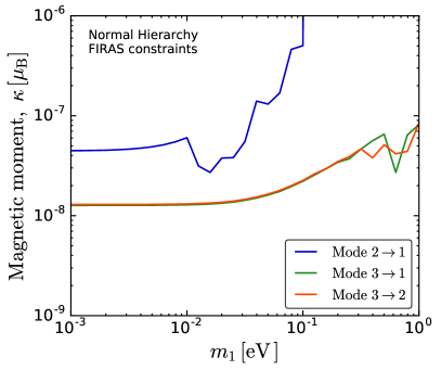
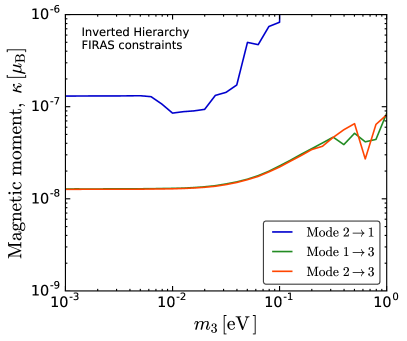
Figure 5: 95% C.L. upper limits on the magnetic moment of neutrinos, as a function of the lightest neutrino mass. Values of the effective transition magnetic moment $\kappa_{ij}$ [defined in Eq. (34)] above the solid lines are excluded by our analysis. Results shown are for NH (left panel) and IH (right panel).

III.3 Comparison to earlier work and degeneracy among parameters

We now compare our results to those previously obtained by Ref. Mirizzi et al. (2007). The analysis of Ref. Mirizzi et al. (2007) did not take into account stimulated emission, Pauli-blocking or absorption, and assumed the neutrinos to be at rest at the moment of decay. In addition, only $\Gamma$ was varied in the $\chi^{2}$ analysis. The difference between these results should tell us the impact of the exact calculation on the CMB spectrum as well as the importance of including additional nuisance parameters in the analysis.

When we compare our exact results to the findings in Ref. Mirizzi et al. (2007), we find that our results are in broad agreement with the results of Fig. 2 presented there. For NH, we obtain a stronger limit for the 12 mode in the range of $10^{-2}\;\mathrm{eV}\lesssim m_{\nu}\lesssim 10^{-1}\;\mathrm{eV}$ by about one order of magnitude. For IH, our bounds on the 13 and 23 modes are slightly weaker (by a factor of around 2) than the bounds found in Ref. Mirizzi et al. (2007) in the region $10^{-3}\;\mathrm{eV}\lesssim m_{\nu}\lesssim 10^{-1}\;\mathrm{eV}$. We again obtain a stronger bound on the 12 mode in the region $10^{-2}\;\mathrm{eV}\lesssim m_{\nu}\lesssim 10^{-1}\;\mathrm{eV}$. We emphasize that we expect our constraints to be more accurate, as we include more accurate calculations of the spectral distortions and more parameters in the analysis.

To further investigate how our results differ from the previous constraints, we have repeated our analysis, following (where possible) the analysis procedure of Ref. Mirizzi et al. (2007). In order to do this, we use the following model for the intensity:

$$I=I_{0}+\Gamma_{ij}I_{ij}^{\mathrm{dec}},$$ (35)

instead of the full model given in Eq. (24), fixing all the other parameters to be zero. Note that we do not include the contribution of absorption or stimulated emission, and calculate the decay intensity using the approximate approach presented in Sec. II.1. The uncertainty on the decay rate is then given by $\sigma_{\Gamma}^{2}=2(\partial^{2}\chi^{2}/\partial\Gamma^{2})^{-1}$ (not taking into account the full Fisher matrix). We also adopt the mass differences and cosmological parameters stated in Ref. Mirizzi et al. (2007).

The resulting lower limits on $\tau$ are shown in Fig. 6, where dashed lines are the bounds reported in Ref. Mirizzi et al. (2007) and solid lines show our bounds using the same analysis approach. The shape of the bounds is in close agreement. However, we notice that our bounds are around one order of magnitude stronger, although we have attempted to reproduce the analysis of Ref. Mirizzi et al. (2007) as closely as possible. Unfortunately, we have not been able to find the source of this discrepancy.

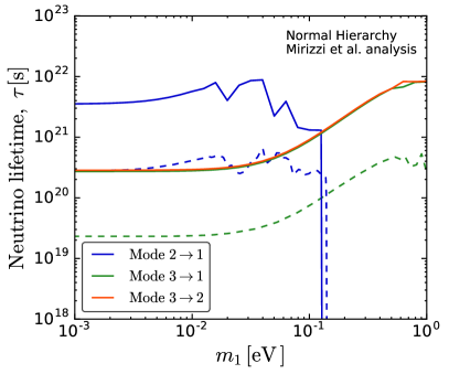
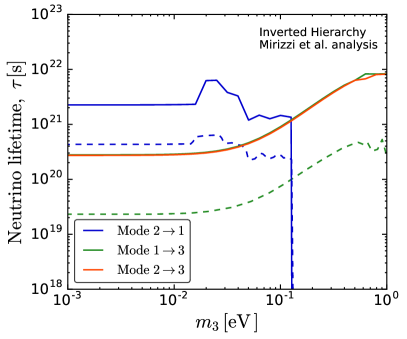
Figure 6: 95% C.L. lower limits on the radiative decay lifetime of neutrinos, following the analysis method of Ref. Mirizzi et al. (2007). These constraints were derived using approximate expressions for neutrino decay only and fixing all nuisance parameters except for $\Gamma$. Dashed lines are the limits reported by Ref. Mirizzi et al. (2007). Results shown are for NH (left panel) and IH (right panel).

Lastly, when comparing our approximate bounds in Fig. 6 with the full analysis from Fig. 4, we notice that the full bounds are typically weaker by a factor of $\sim$30. This implies that we cannot ignore the correlation among different parameters (which are included in the full analysis). To see the effect more quantitatively, we introduce the correlation coefficients:

$$\rho(\theta_{a},\theta_{b})\equiv\frac{\mbox{Cov}(\theta_{a},\theta_{b})}{\sigma_{a}\sigma_{b}},$$ (36)

and show them between $\Gamma_{ij}$ and the other parameters in Fig. 7 for the modes 12 and 13 and for both the NH and IH (those for the mode 23 is almost identical to those for 13). In fact, we find very strong anti-correlation between $\Gamma_{13}$ (or $\Gamma_{23}$) and the Galactic component $G_{0}$ as well as the $y$-distortion for nearly all the masses investigated here. This is because the modification of the CMB spectrum increases as a function of the frequency without any feature, and is thus indistinguishable from the Galactic residual component found in Ref. Fixsen et al. (1996) up to the FIRAS errors. On the other hand, if a sharp spectral feature appears in the FIRAS frequency range (as is the case for $m_{1}\in[10^{-2},10^{-1}]\;\mathrm{eV}$ in the 12 mode), it breaks the degeneracy and hence the anti-correlation disappears (upper left panel of Fig. 7). Indeed, we see that comparing the full (Fig. 4) and approximate analysis (Fig. 6), the bounds in this mass range are largely unchanged between the two.

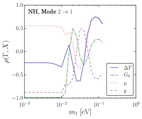
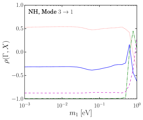
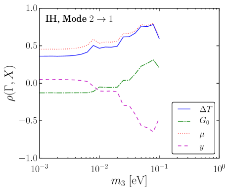
Figure 7: Correlation coefficients $\rho(\Gamma,X)$ between the decay rate $\Gamma$ and other parameters $X\in\{\Delta T,G_{0},\mu,y\}$. The correlation coefficients [Eq. (36)] are shown as a function of the lightest neutrino mass, for NH (top row) and IH (bottom row) and for the modes 12 (left column) and 13 (right column).

These results show that in the full analysis, including $\theta_{a}\in\{\Delta T,\mu,G_{0},y,\Gamma_{ij}\}$, degeneracies between the parameters can substantially weaken constraints on the neutrino decay rates $\Gamma_{ij}$. While accounting for these degeneracies represents the most conservative approach, we could alternatively have chosen to fix $\mu=0$ and $y=0$ in the analysis. In the standard $\Lambda$CDM cosmology, we expect $y\in[10^{-7},10^{-6}]$, caused by heating during reionization and other heating mechanisms Hu et al. (1994); Refregier et al. (2000); Oh et al. (2003) and $\mu\sim\mathcal{O}(10^{-8})$, from the damping of primordial fluctatuations Hu and Silk (1993a). These values lie below the FIRAS sensitivity and so, if we assume no other sources of $\mu$- and $y$-distortions, we could keep these parameters fixed (effectively to zero) in the analysis. The solid lines in Fig. 6 give an estimate of the limits on $\Gamma_{ij}$ in this case. As we discuss in the next section, future experiments will be more sensitive to $\mu$ and $y$, in which case their inclusion in the analysis is unavoidable.

IV Sensitivity of future CMB experiments

Highly sensitive future CMB measurements will be able to measure spectral distortions to a high degree of precision. Of particular interest are $\mu$- and $y$-distortions, briefly discussed in the previous section. These provide information about energy-release at certain redshifts and therefore allow us to constrain the thermal history of the Universe Chluba (2013). A measurement of $y$-distortions may provide information about structure formation and the epoch of reionization at $z<10$–20, as well as allowing us to probe the primordial power spectrum on small scales Sunyaev and Zeldovich (1970). The decay and annihilation of particles in the pre-recombination epoch ($5\times 10^{4}<z<2\times 10^{6}$) may give rise to $\mu$-distortions Hu and Silk (1993b), providing sensitivity to particle lifetimes in the range $\tau\simeq 10^{8}$–$10^{11}$ s. As we have explored so far in this work, particles with longer lifetimes may also distort the CMB spectrum and provide a detectable signal in future CMB experiments.

Here we focus on the PIXIE mission which is expected to cover a frequency range of 30 GHz (1 cm^-1) to 6 THz (200 cm^-1), using 400 channels. For this analysis, however, we will only look at a range 30–750 GHz (1–25 cm^-1, divided into 48 frequency bins), as most of the CMB spectrum lies within this range. Furthermore, at frequencies higher than 3 THz, the spectrum is dominated by dust emitting foregrounds that do not affect the final analysis Abitbol et al. (2017).

Following closely the analysis of Sec. III, we obtain projected lower limits on the neutrino lifetime $\tau$ from the PIXIE experiment. We assume that the error on the intensity in each frequency bin is 5 Jy/sr Kogut et al. (2011b), and that there are no correlations between the different frequency bins. We include the parameters $\theta_{a}\in\{\Delta T,\mu,G_{0},y,\Gamma_{ij}\}$ in the modeled intensity, with the projected Galactic contamination taken from Ref. Abitbol et al. (2017). We also consider the ideal case in which $G_{0}$ is fixed to zero; i.e., the Galactic contamination, presumably calibrated with other wavebands, is well constrained and perfectly subtracted.

Unlike in Sec. III, the intensity spectrum has not yet been measured by PIXIE. We therefore assume that the best fit decay rate will be $\hat{\Gamma}=0$. Using the Fisher-matrix approach of Sec. III, we then estimate the 95% C.L. projected limit on $\Gamma$ as $\Gamma^{95\%}\approx 1.64\sigma_{\Gamma}$, where $\sigma_{\Gamma}$ is defined in Eq. (31). As noted in Sec. III.1, in our linearised intensity model the numerical value of the Fisher matrix does not depend on the model parameters $\theta_{a}$. This means that the projection we obtain for $\Gamma^{95\%}$ does not depend on the assumed values of the nuisance parameters (although it would depend on the assumed best fit of the decay rate $\hat{\Gamma}$).

The PIXIE projected limits are shown in Fig. 8. Solid lines show the projections including parameters $\theta_{a}\in\{\Delta T,\mu,G_{0},y,\Gamma_{ij}\}$, while dotted lines show the projection when $G_{0}$ is fixed to zero. The qualitative behavior of the bounds matches those from FIRAS, although for the 12 mode the bounds extend to higher values of $m_{1}$ as PIXIE will probe down to lower frequencies than FIRAS. The projected limits lie in the range $\tau\gtrsim 10^{23}$–$10^{25}$ s, representing a factor of $10^{4}$ improvement over the FIRAS limits. This improvement arises both from a reduction of the uncertainties on the CMB intensity and from an increase in the number of frequency channels from FIRAS to PIXIE. Fixing the Galactic component to zero improves the constraints by roughly another order of magnitude (unless the spectral feature lies within the PIXIE frequency range, as is the case for masses above $10^{-2}$ eV in the 12 mode).

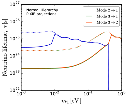
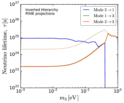
Figure 8: Projected 95% C.L. lower limits on radiative decay lifetime of neutrinos as a function of the lightest neutrino mass for a PIXIE-like experiment. Dotted lines correspond to the lower limits assuming that the residual Galactic contamination $G_{0}$ is fixed to zero. Left panel: Results for NH, where $m_{1}$ is the lowest mass. Right panel: Results for IH where $m_{3}$ is the lowest mass.

We convert the projected upper limits on the neutrino lifetime into limits on the neutrino transition magnetic and electric moments $\kappa_{ij}$. The result is shown in Fig. 9, where again dotted lines show the case where the Galactic component is kept fixed. The factor of $10^{4}$ improvement in neutrino lifetime constraints translates to a factor of $10^{2}$ improvement in the magnetic moment constraints. For the lightest neutrino masses below 0.1 eV, the limit on $\kappa$ ranges from $10^{-8}\;\mu_{B}$ down to $3\times 10^{-11}\;\mu_{B}$, depending on the hierarchy and assumptions about Galactic contamination. In particular, we note that for the 23 mode, lightest neutrino mass lower than $10^{-2}$ eV and minimal Galactic contamination, constraints from a PIXIE-like experiment may be competitive with the best lab-based $\nu$–$e$ scattering experiments (cf., constraints from BOREXINO give $\mu_{\nu}<2.8\times 10^{-11}\mu_{B}$ Agostini et al. (2017b) at 90% C.L.).

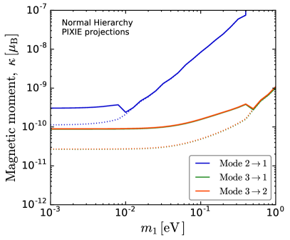
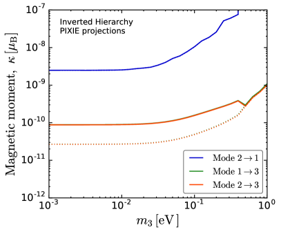
Figure 9: Projected 95% C.L. upper limits on the magnetic moment of neutrinos, as a function of the lightest neutrino mass for a PIXIE-like experiment. The effective transition magnetic moment $\kappa_{ij}$ is related to the decay rate $\Gamma_{ij}$ by Eq. (34). Dotted lines correspond to the upper limits assuming that the residual Galactic contamination $G_{0}$ is fixed to zero. Results shown are for NH (left panel) and IH (right panel).

V Conclusions

In this work, we have presented updated constraints on the neutrino radiative decay lifetime $\tau$ from FIRAS measurements of the CMB intensity spectrum, introducing a number of refinements compared to previous work Mirizzi et al. (2007). We include spectral distortions from photon absorption by neutrinos (not only from neutrino decays), as well as calculating decay and absorption rates taking into account the momentum distribution of the cosmic neutrino background. In our analysis, we simultaneously fit the neutrino decay rate $\Gamma=1/\tau$ along with other nuisance parameters, including the temperature deviation $\Delta T$, $\mu$- and $y$-distortions and the residual Galactic contamination $G_{0}$. These lead to more accurate and robust limits than previously presented.

We find that the effects of absorption and decay are comparable for neutrino masses $\mathcal{O}(0.1)\,\mathrm{eV}$ and larger. We also find that the approximate formalism (assuming that the cosmic neutrinos are at rest) may overestimate the spectral distortions by around 50%. Finally, we find strong anti-correlation between the decay rate $\Gamma$ and the other nuisance parameters in the analysis, weakening the constraints on the neutrino lifetime unless a clear spectral feature is produced in the FIRAS frequency range (as is that case where the lightest mass lies in $[10^{-2},10^{-1}]\,\mathrm{eV}$ for the 12 mode). While these effects should tend to weaken our constraints, we in fact find stronger constraints than previous analyses Mirizzi et al. (2007), in some cases by around an order of magnitude, although the source of this discrepancy is not clear. In particular, we find $\tau_{12}\gtrsim 4\times 10^{21}\,\mathrm{s}$ for the 12 decay mode in the normal hierarchy and $\tau_{12}\gtrsim 10^{22}\,\mathrm{s}$ in the inverted hierarchy. For the 13 and 23 modes, there are no sharp spectral features in the FIRAS frequency range, leading to weaker limits, $\tau_{13}\sim\tau_{23}\gtrsim 10^{19}\,\mathrm{s}$. The corresponding constraints on the neutrino magnetic moment lie in the range $10^{-8}$–$10^{-7}\,\mu_{B}$.

We have also explored projected constraints from future precision CMB spectral measurements, focusing on the proposed PIXIE experiment Kogut et al. (2011a). With an improvement in measurement sensitivity of around three orders of magnitude compared to FIRAS, PIXIE should be able to constrain the radiative decay lifetime of the neutrino at the level of $\tau\gtrsim 10^{23}$–$10^{25}\,\mathrm{s}$ depending on the neutrino mass and hierarchy. If residual Galactic contamination in the CMB spectrum is well constrained, a PIXIE-like experiment may probe magnetic moments down to $\kappa\lesssim 3\times 10^{-11}\,\mu_{B}$ for the 13 and 23 modes. While still one order of magnitude weaker than constraints from stellar physics Raffelt (1990, 1999); Arceo-Díaz et al. (2015), such a constraint would be competitive with current lab-based constraints from $\nu$–$e$ scattering measurements Beda et al. (2013); Agostini et al. (2017a). Further improvements in sensitivity, as proposed by the PRISM experiment Andre et al. (2013), would lead to still stronger bounds on the neutrino lifetime and magnetic moment, making precision CMB spectral measurements a competitive and complementary tool for probing New Physics in the neutrino sector.

Appendix A Emissivity of photons

In this section, we derive exact formulae for decay and absorption intensities without making any assumptions.

A.1 Decay

From kinematics of the decay $\nu_{j}\to\nu_{i}+\gamma$, one obtains

$$p_{\gamma}=p_{\gamma}^{d}(p_{\nu},\mu)\equiv\frac{\Delta m_{ij}^{2}}{2\left(\sqrt{p_{\nu}^{2}+m_{j}^{2}}-p_{\nu}\mu\right)}$$ (37)

where $p_{\nu}=|\bm{p}_{\nu}|$, $p_{\gamma}=|\bm{p}_{\gamma}|$, $\bm{p}_{\nu}$ and $\bm{p}_{\gamma}$ are the momentum of $\nu_{j}$ and $\gamma$, respectively, and $\mu=\bm{p}_{\nu}\cdot\bm{p}_{\gamma}/(p_{\nu}p_{\gamma})$. Alternatively, rewriting Eq. (37) for $\mu$ gives

$$\mu=\mu_{d}(p_{\gamma},p_{\nu})\equiv\sqrt{1+\frac{m_{j}^{2}}{p_{\nu}^{2}}}-\frac{\Delta m_{ij}^{2}}{2p_{\nu}p_{\gamma}}.$$ (38)

In order for the decay to happen, the variables and parameters $(p_{\nu},p_{\gamma},m_{j},\Delta m_{ij}^{2})$ have to satisfy $\mu_{d}^{2}<1$. The momentum of the final-state neutrino $\nu_{i}$ is then obtained as

$$p_{\nu_{i}}^{d}(p_{\gamma},p_{\nu})=\sqrt{p_{\gamma}^{2}+p_{\nu}^{2}-2p_{\gamma}p_{\nu}\mu_{d}(p_{\gamma},p_{\nu})}.$$ (39)

The photon emissivity at energy $p_{\gamma}$ is obtained as a similar equation as Eq. (14) but by replacing the neutrino number density with the neutrino phase space density integrated over momentum space:

$$P_{\rm dec}(p_{\gamma}) = \frac{g_{\nu}}{(2\pi)^{2}}\int\frac{d^{3}p_{\nu}}{e^{p_{\nu}/T_{\nu}}+1}\frac{m_{j}\Gamma}{\sqrt{p_{\nu}^{2}+m_{j}^{2}}}$$ (40)

$$\times p_{\gamma}\delta\left(p_{\gamma}-p_{\gamma}^{d}(p_{\nu},\mu)\right)(1+f_{\rm CMB}(p_{\gamma}))$$

$$\times\left[1-\frac{1}{e^{p_{\nu_{i}}^{d}(p_{\gamma},p_{\nu})/T_{\nu}}+1}\right],$$

$$= \frac{\Gamma m_{j}\Delta m_{\ij}^{2}}{4\pi^{2}}\frac{1+f_{\rm CMB}(p_{\gamma})}{p_{\gamma}}$$

$$\times\int_{0}^{\infty}\frac{dp_{\nu}p_{\nu}}{(e^{p_{\nu}/T_{\nu}}+1)\sqrt{p_{\nu}^{2}+m_{j}^{2}}}$$

$$\times\left[1-\frac{1}{e^{p_{\nu_{i}}^{d}(p_{\gamma},p_{\nu})/T_{\nu}}+1}\right]$$

$$\times\int_{-1}^{1}d\mu\delta\left(\mu-\mu_{d}(p_{\gamma},p_{\nu})\right),$$

where $g_{\nu}=2$ is the number of helicities of the neutrino, the lifetime of $\nu_{j}$ is longer than its proper lifetime $\tau$ by a Lorentz factor of $(p_{\nu}^{2}+m_{j}^{2})^{1/2}/m_{j}$, the stimulated emission is taken into account with the term $1+f_{\rm CMB}(p_{\gamma})$, and the term in the square bracket represents the Pauli blocking for the final neutrino state with momentum $p_{\nu_{i}}^{d}$. In the second equality, we changed the $\delta$-function of $p_{\gamma}$ to that of $\mu$, by using $\delta\left(p_{\gamma}-p_{\gamma}^{d}\right)=\left|{\partial p_{\gamma}^{d}}/{\partial\mu}\right|^{-1}\delta\left(\mu-\mu_{d}\right)$, and $|\partial p_{\gamma}^{d}/\partial\mu|=2p_{\gamma}^{2}p_{\nu}/\Delta m_{ij}^{2}$.

The $\mu$-integral over its $\delta$-function gives nonzero value (i.e., 1) only if $\mu_{d}^{2}<1$. By rearranging Eq. (38), we find the condition to be equivalent to $x>|t-t^{-1}|y/2$, where $x=p_{\nu}/T_{\nu}$, $y=m_{j}/T_{\nu}$, and $t=2p_{\gamma}m_{j}/\Delta m_{ij}^{2}$. We also note $\mu_{d}=\left[(x^{2}+y^{2})^{1/2}-y/t\right]/x$.

Finally, we evaluate the emissivity at redshift $z$ and observed energy of $\epsilon_{\gamma}$. We can use all the equations derived thus far with replacements: $p_{\gamma}\to(1+z)\epsilon_{\gamma}$, $p_{\nu}\to(1+z)p_{\nu}$, and $T_{\nu}\to(1+z)T_{\nu}$. The emissivity of the neutrino decay is then obtained as Eq. (19).

A.2 Absorption

For the absorption $\nu_{i}+\gamma\to\nu_{j}$, the kinematics relations are

$$p_{\gamma} = p_{\gamma}^{a}(p_{\nu},\mu)\equiv\frac{\Delta m_{ij}^{2}}{2\left(\sqrt{p_{\nu}^{2}+m_{i}^{2}}-p_{\nu}\mu\right)},$$ (41)

$$\mu = \mu_{a}(p_{\gamma},p_{\nu})\equiv\sqrt{1+\frac{m_{i}^{2}}{p_{\nu}^{2}}}-\frac{\Delta m_{ij}^{2}}{2p_{\nu}p_{\gamma}},$$ (42)

where $p_{\nu}$ is (norm of) the momentum of $\nu_{i}$; definitions of the other quantities are the same as the case of decay. The momentum of the final-state neutrino $\nu_{j}$ is then

$$p_{\nu_{j}}^{a}(p_{\gamma},p_{\nu})=\sqrt{p_{\gamma}^{2}+p_{\nu}^{2}+2p_{\gamma}p_{\nu}\mu_{a}(p_{\gamma},p_{\nu})}.$$ (43)

The center-of-mass energy of the initial state $E$ is given by $E^{2}=m_{i}^{2}+2p_{\gamma}\left[(p_{\nu}^{2}+m_{i}^{2})^{1/2}-p_{\nu}\mu\right]$, and the $\delta$-function of $E$ can be replaced with that of $\mu$ through $\delta(E-m_{j})=|\partial E/\partial\mu|^{-1}\delta(\mu-\mu_{a})$ with $|\partial E/\partial\mu|=p_{\gamma}p_{\nu}/m_{j}$. The absorption cross section [Eq. (5)] then becomes

$$\sigma(p_{\gamma},p_{\nu},\mu)=\frac{4\pi^{2}m_{j}^{3}\Gamma}{(\Delta m_{ij}^{2})^{2}p_{\gamma}p_{\nu}}\delta(\mu-\mu_{a}).$$ (44)

The absorption emissivity is given as product of the phase space densities of both $\gamma$ and $\nu_{i}$, multiplied by the absorption cross section as follows:

$$P_{\rm abs}(p_{\gamma})dp_{\gamma} = -p_{\gamma}\frac{g_{\gamma}}{(2\pi)^{3}}f_{\rm CMB}(p_{\gamma})d^{3}p_{\gamma}$$ (45)

$${}\times\frac{g_{\nu}}{(2\pi)^{3}}\int\frac{d^{3}p_{\nu}}{e^{p_{\nu}/T_{\nu}}+1}\sigma(p_{\gamma},p_{\nu},\mu)$$

$${}\times\left[1-\frac{1}{e^{p_{\nu_{j}}^{a}(p_{\gamma},p_{\nu})/T_{\nu}}+1}\right],$$

where $g_{\gamma}=2$ is the number of polarization states of the photon. Using Eq. (44) and performing the $\mu$-integral over the $\delta$-function that yields a nonzero value only when $\mu_{a}^{2}<1$, one obtains

$$P_{\rm abs}(p_{\gamma}) = -\frac{2}{\pi^{2}}\frac{m_{j}^{3}\Gamma}{(\Delta m_{ij}^{2})^{2}}p_{\gamma}^{2}f_{\rm CMB}(p_{\gamma})$$ (46)

$${}\times\int_{0}^{\infty}\frac{dp_{\nu}p_{\nu}}{e^{p_{\nu}/T_{\nu}}+1}\Theta\left(1-\mu_{a}^{2}\right(p_{\gamma},p_{\nu}))$$

$${}\times\left[1-\frac{1}{e^{p_{\nu_{j}}^{a}(p_{\gamma},p_{\nu})/T_{\nu}}+1}\right],$$

where $\Theta$ is the Heaviside step function. As in the case of decay, this constraint, $\mu_{a}^{2}<1$, is equivalent to $x>|t-t^{-1}|y/2$, with $x=p_{\nu}/T_{\nu}$, $y=m_{i}/T_{\nu}$, and $t=2p_{\gamma}m_{i}/\Delta m_{ij}^{2}$.

Lastly, with replacements $p_{\gamma}\to(1+z)\epsilon_{\gamma}$, $p_{\nu}\to(1+z)p_{\nu}$, $T_{\rm CMB}\to(1+z)T_{\rm CMB}$, and $T_{\nu}\to(1+z)T_{\nu}$, we arrive at Eq. (20).

References

- Patrignani et al. (2016) C. Patrignani et al. (Particle Data Group), Chin. Phys. C40, 100001 (2016).
- Giganti et al. (2018) C. Giganti, S. Lavignac, and M. Zito, Prog. Part. Nucl. Phys. 98, 1 (2018), arXiv:1710.00715 [hep-ex] .
- Qian and Vogel (2015) X. Qian and P. Vogel, Prog. Part. Nucl. Phys. 83, 1 (2015), arXiv:1505.01891 [hep-ex] .
- Hagedorn et al. (2017) C. Hagedorn, R. N. Mohapatra, E. Molinaro, C. C. Nishi, and S. T. Petcov, (2017), arXiv:1711.02866 [hep-ph] .
- Levine (1967) M. J. Levine, Il Nuovo Cimento A Series 10 48, 67 (1967).
- Cung and Yoshimura (1975) V. K. Cung and M. Yoshimura, Il Nuovo Cimento A 29, 557 (1975).
- Pal and Wolfenstein (1982) P. B. Pal and L. Wolfenstein, Phys. Rev. D25, 766 (1982).
- Fujikawa and Shrock (1980) K. Fujikawa and R. E. Shrock, Phys. Rev. Lett. 45, 963 (1980).
- Glashow et al. (1970) S. L. Glashow, J. Iliopoulos, and L. Maiani, Physical Review D 2, 1285 (1970).
- Beda et al. (2013) A. G. Beda, V. B. Brudanin, V. G. Egorov, D. V. Medvedev, V. S. Pogosov, E. A. Shevchik, M. V. Shirchenko, A. S. Starostin, and I. V. Zhitnikov, Phys. Part. Nucl. Lett. 10, 139 (2013).
- Agostini et al. (2017a) M. Agostini et al. (Borexino), Phys. Rev. D96, 091103 (2017a), arXiv:1707.09355 [hep-ex] .
- Raffelt (1990) G. G. Raffelt, Phys. Rev. Lett. 64, 2856 (1990).
- Raffelt (1999) G. G. Raffelt, Phys. Rept. 320, 319 (1999).
- Arceo-Díaz et al. (2015) S. Arceo-Díaz, K. P. Schröder, K. Zuber, and D. Jack, Astropart. Phys. 70, 1 (2015).
- Studenikin (2016) A. Studenikin, Proceedings, 14th International Conference on Topics in Astroparticle and Underground Physics (TAUP 2015): Torino, Italy, September 7-11, 2015, J. Phys. Conf. Ser. 718, 062076 (2016), arXiv:1603.00337 [hep-ph] .
- Studenikin (2018) A. Studenikin, in 2017 European Physical Society Conference on High Energy Physics (EPS-HEP 2017) Venice, Italy, July 5-12, 2017 (2018) arXiv:1801.08887 [hep-ph] .
- Shrock (1974) R. Shrock, Phys. Rev. D9, 743 (1974).
- Lee and Shrock (1977) B. W. Lee and R. E. Shrock, Phys. Rev. D16, 1444 (1977).
- Shrock (1982) R. E. Shrock, Nucl. Phys. B206, 359 (1982).
- Georgi and Randall (1990) H. Georgi and L. Randall, Phys. Lett. B244, 196 (1990).
- Davidson et al. (2005) S. Davidson, M. Gorbahn, and A. Santamaria, Phys. Lett. B626, 151 (2005), hep-ph/0506085 .
- Bell et al. (2005) N. F. Bell, V. Cirigliano, M. J. Ramsey-Musolf, P. Vogel, and M. B. Wise, Phys. Rev. Lett. 95, 151802 (2005), hep-ph/0504134 .
- Bell et al. (2006) N. F. Bell, M. Gorchtein, M. J. Ramsey-Musolf, P. Vogel, and P. Wang, Phys. Lett. B642, 377 (2006), arXiv:hep-ph/0606248 [hep-ph] .
- Frère et al. (2015) J.-M. Frère, J. Heeck, and S. Mollet, Phys. Rev. D92, 053002 (2015), arXiv:1506.02964 [hep-ph] .
- Lindner et al. (2017) M. Lindner, B. Radovčić, and J. Welter, JHEP 07, 139 (2017), arXiv:1706.02555 [hep-ph] .
- Ade et al. (2016) P. A. R. Ade et al. (Planck), Astron. Astrophys. 594, A13 (2016), arXiv:1502.01589 [astro-ph.CO] .
- Gando et al. (2016) A. Gando et al. (KamLAND-Zen), Phys. Rev. Lett. 117, 082503 (2016), [Addendum: Phys. Rev. Lett.117, no.10, 109903 (2016)], arXiv:1605.02889 [hep-ex] .
- Mirizzi et al. (2007) A. Mirizzi, D. Montanino, and P. D. Serpico, Phys. Rev. D76, 053007 (2007), arXiv:0705.4667 [hep-ph] .
- Fixsen et al. (1996) D. J. Fixsen, E. S. Cheng, J. M. Gales, J. C. Mather, R. A. Shafer, and E. L. Wright, Astrophys. J. 473, 576 (1996), astro-ph/9605054 .
- Fixsen and Mather (2002) D. J. Fixsen and J. C. Mather, Astrophys. J. 581, 817 (2002).
- Masso and Toldra (1999) E. Masso and R. Toldra, Phys. Rev. D60, 083503 (1999), astro-ph/9903397 .
- Kogut et al. (2011a) A. Kogut, D. J. Fixsen, D. T. Chuss, J. Dotson, E. Dwek, M. Halpern, G. F. Hinshaw, S. M. Meyer, S. H. Moseley, M. D. Seiffert, D. N. Spergel, and E. J. Wollack, Journal of Cosmology and Astroparticle Physics 7, 025 (2011a), arXiv:1105.2044 .
- Chluba and Jeong (2014) J. Chluba and D. Jeong, Mon. Not. Roy. Astron. Soc. 438, 2065 (2014), arXiv:1306.5751 [astro-ph.CO] .
- Andre et al. (2013) P. Andre et al. (PRISM), (2013), arXiv:1306.2259 [astro-ph.CO] .
- Peacock (1999) J. A. Peacock, Cosmological Physics (1999).
- Wong (2011) Y. Y. Y. Wong, Ann. Rev. Nucl. Part. Sci. 61, 69 (2011), arXiv:1111.1436 [astro-ph.CO] .
- Zeldovich and Sunyaev (1969) Y. B. Zeldovich and R. A. Sunyaev, Astrophysics and Space Science 4, 301 (1969).
- Raffelt (1996) G. G. Raffelt, Stars as Laboratories for Fundamental Physics (Chicago, USA: Univ. Pr. (1996) 664 p, 1996).
- Hu et al. (1994) W. Hu, D. Scott, and J. Silk, Phys. Rev. D49, 648 (1994), arXiv:astro-ph/9305038 [astro-ph] .
- Refregier et al. (2000) A. Refregier, E. Komatsu, D. N. Spergel, and U.-L. Pen, Phys. Rev. D61, 123001 (2000), arXiv:astro-ph/9912180 [astro-ph] .
- Oh et al. (2003) S. P. Oh, A. Cooray, and M. Kamionkowski, Mon. Not. Roy. Astron. Soc. 342, L20 (2003), arXiv:astro-ph/0303007 [astro-ph] .
- Hu and Silk (1993a) W. Hu and J. Silk, Phys. Rev. D48, 485 (1993a).
- Chluba (2013) J. Chluba, Mon. Not. Roy. Astron. Soc. 436, 2232 (2013), arXiv:1304.6121 [astro-ph.CO] .
- Sunyaev and Zeldovich (1970) R. A. Sunyaev and Y. B. Zeldovich, Astrophysics and Space Science 7, 3 (1970).
- Hu and Silk (1993b) W. Hu and J. Silk, Physical Review Letters 70, 2661 (1993b).
- Abitbol et al. (2017) M. H. Abitbol, J. Chluba, J. C. Hill, and B. R. Johnson, Mon. Not. Roy. Astron. Soc. 471, 1126 (2017), arXiv:1705.01534 [astro-ph.CO] .
- Kogut et al. (2011b) A. Kogut, D. J. Fixsen, D. T. Chuss, J. Dotson, E. Dwek, M. Halpern, G. F. Hinshaw, S. M. Meyer, S. H. Moseley, M. D. Seiffert, D. N. Spergel, and E. J. Wollack, JCAP 7, 025 (2011b), arXiv:1105.2044 .
- Agostini et al. (2017b) M. Agostini et al. (Borexino), Phys. Rev. D96, 091103 (2017b), arXiv:1707.09355 [hep-ex] .