Abstract

We study stringy modifications of $T^{3}$–fibered manifolds, where the fiber undergoes a monodromy in the T–duality group. We determine the fibration data defining such T–folds from a geometric model, by using a map between the duality group and the group of large diffeomorphisms of a four-torus. We describe the monodromies induced around duality defects where such fibrations degenerate and we argue that local solutions receive corrections from the winding sector, dual to the symmetry–breaking modes that correct semi–flat metrics.

1 Introduction

In exploring the space of string compactifications it is practical to consider a boundary of the moduli space where volume moduli have become very large, and supergravity is the correct low-energy theory governing the light modes. However, many interesting string vacua, that populate the interior of the moduli space, cannot be analyzed in this way. In particular, this restriction precludes the study of truly stringy geometries, where the large symmetry group of string theory is expected to modify the notion of Riemannian geometry. Examples of such compactifications are constructed by modifying the familiar semi-flat SYZ fibrations of Calabi-Yau manifolds [1], allowing the torus fiber to undergo monodromies in the full U-duality group. The resulting spaces are usually referred to as T-folds [2, 3, 4] (when the monodromies are restricted to the T-duality group) or U-folds [5, 6, 7].

In order to determine if such spaces are good string backgrounds one needs to have control on the corrections to the supergravity approximation and to have a microscopic description of the defects where the semi-flat approximation breaks down. These are non-geometric defects that induce a monodromy in the duality group [8, 9]. A way to deal with the first problem is to use string dualities in order relate the T-duality group with the group of large diffeomorphisms of a manifold that is part of a known string compactification, in the spirit of F-theory [10]. This can be done, for example, for T-folds in the heterotic strings [11, 12, 13]. The duality map can then be used to compute the low energy dynamics on the T-duality defects [14, 15].

So far, the only known examples of such non-geometric fibrations are six-dimensional and involve a stringy modification of $T^{2}$ fibered K3 surfaces, with the exception of asymmetric orbifold points in the moduli space of $T^{3}$ fibered T-folds [4].

In this note we consider an explicit globally well defined example of a T-fold that admits a $T^{3}$ fibration, by realizing a subset of the T-duality group $O(3,3;\mathbb{Z})$ as the group of large diffeomorphisms of a $T^{4}$. We use known families of $T^{4}$ fibered Calabi-Yau manifolds to construct a family of such T-folds. In the geometric picture, the local defects are simply Taub-NUT spaces, and get dualized to non-geometric defects that are T-dual to NS5 branes. Such T-duality cannot be extended globally because of topological twists in the global fibration. We also use the above mentioned map to construct a geometric description of the non-geometric $T^{2}$ fibrations of [2]. In order to get to such a geometric model one needs to add an extra circle, which is related by duality to the M-theory circle [4]. We will also argue that the local physics on non-geometric defects cannot be fully captured by such geometric constructions, and involve stringy physics related to the sector of strings winding cycles in the fiber.

While we will restrict to the case of a two-dimensional base, we have in mind extensions of these models to the interesting case of $T^{3}$ fibrations over a three-dimensional base. In appendix B we briefly discuss an attempt in this direction.

2 Monodromy and duality group

A useful way to construct candidate non-geometric string compactifications is to use an adiabatic fibration of a CFT on a torus $T^{d}$ over a base $\mathcal{B}$. Any two theories related by a T-duality transformation of the fiber in $\mathcal{G}_{d}=O(d,d;\mathbb{Z})$ are gauge equivalent (see for example [16] for a review on T-duality), and hence it should be possible to allow for large gauge transformations in $\mathcal{G}_{d}$. Generically these involve a non-trivial action on the fiber volume, and so the total space is a non-geometric T-fold. The notion of a T-fold is not rigorous in general, but we will give a precise construction in special cases, restricting ourselves to $T^{3}$ bundles. Following [9], we will define T-folds with base manifold a circle and then extend this definition to spheres with $n$ punctures.

2.1 Mapping tori for $\mathcal{G}_{3}$

The simplest examples of T-folds $\mathcal{X}$ with $T^{3}$ fibers can be constructed by modifying the mapping torus for the mapping class group $SL(3,\mathbb{Z})$. Let us consider a $T^{3}$ fibration over the closed interval $[0,1]$ and making an identification as follows:

$$\mathcal{X}=\frac{T^{3}\times[0,1]}{(x,0)\sim(\phi(x),1)}\,.$$ (2.1)

We refer to $\phi\in SL(3;\mathbb{Z})$ as the monodromy of the fibration. It acts on $H_{1}(T^{3};\mathbb{Z})$ in the obvious way. Depending on the conjugacy class of the monodromy, the total space $\mathcal{X}$ can acquire the structure of a nil- or a sol-manifold (see for example [17]). We pick a Riemannian metric on the total space with line element

$$ds^{2}=d\theta^{2}+G_{ab}(\theta)dx^{a}dx^{b}\,,\quad a,b=1,2,3\,.$$ (2.2)

One readily shows that the (smooth) metric satisfies

$$\phi^{T}G(0)\phi=G(1)\,,$$ (2.3)

where we further restrict ourselves to monodromies $\phi\in SL(3;{\mathbb{Z}})\cap\exp\left(\mathfrak{sl}(3;{\mathbb{R}})\right)$. One then choses a smooth family of metrics $G(\theta)$ on the $T^{3}$ fibers as follows:

$$G(\theta)=\exp\left(\theta\log\phi\right)\cdot G(0)\equiv\left[\exp\left(\theta\log\phi\right)\right]^{T}G(0)\left[\exp\left(\theta\log\phi\right)\right].$$ (2.4)

We define a T-fold by generalizing this construction to monodromies in the T-duality group $\mathcal{G}_{3}=O(3,3;\mathbb{Z})$. In order to make sense of the definition of $\mathcal{X}$ we specify a metric $G$ and a two-form $B$-field on the total space by defining them on each $T_{\theta}^{3}$ fiber over the interval. i.e. we obtain a family of metrics and two-forms on the fibers $G(\theta)$, $B(\theta)$, $\theta\in[0,1]$. We restrict $\phi\in O(3,3;\mathbb{Z})\cap\exp\left(\mathfrak{o}(3,3;{\mathbb{R}})\right)$ and we define the T-duality action in terms of the background matrix $E(\theta)=G(\theta)+B(\theta)$:

$$E(\theta)=\exp\left(\theta\log\phi\right)\cdot E(0)\equiv\frac{X(\theta)E(0)+Y(\theta)}{Z(\theta)E(0)+W(\theta)}\,,$$ (2.5)

where

$$\exp\left(\theta\log\phi\right)=\begin{pmatrix}X(\theta)&Y(\theta)\\ Z(\theta)&W(\theta)\end{pmatrix}\,.$$ (2.6)

Note that the image of the exponential map $\exp:\mathfrak{o}(3,3;{\mathbb{R}})\rightarrow O(3,3;{\mathbb{R}})$ is contained in the subgroup $SO(3,3;{\mathbb{R}})^{+}$. Recall that $SO(3,3;\mathbb{Z})$ is generated by the following type of transformations:

• Large diffeomorphisms. These are elements of the form

  $$\left(\begin{array}[]{cc}(R^{-1})^{T}&0\\ 0&R\end{array}\right),\ \ \ R\in GL(3;\mathbb{Z}).$$ (2.7)

  These act on $E$ by conjugation.

• $B$-shifts and $\beta$ transformations. $B$-shifts are of the form

  $$\begin{pmatrix}\mathbb{E}_{3}&\Theta\\ 0&\mathbb{E}_{3}\end{pmatrix}\,,\quad\Theta^{T}=-\Theta,$$ (2.8)

  and are just gauge transformations for the $B$-field, $B_{ij}\mapsto B_{ij}+\Theta_{ij}$. $\beta$-transformations on the other hand are transpositions of shifts

  $$\begin{pmatrix}\mathbb{E}_{3}&0\\ \omega&\mathbb{E}_{3}\end{pmatrix}\,,\quad\omega^{T}=-\omega,$$ (2.9)

  and they mix the metric and $B$-field.

• Factorized dualities. These are of the form

  $$\begin{pmatrix}\mathbb{E}_{3}-E_{ii}&E_{ii}\\ E_{ii}&\mathbb{E}_{3}-E_{ii}\end{pmatrix}$$ (2.10)

  where $E_{ii}$ is an elementary matrix, i.e. it has entries $(E_{ii})_{kl}=\delta_{ik}\delta_{il}$.

Note that for shifts and geometric monodromies one obtains a well-defined Riemannian manifold $\mathcal{X}$ over $S^{1}$ with an $H$ flux. We will refer to $\mathcal{X}$ as geometric if the monodromy $\phi$ is comprised of shifts and diffeomorphisms. Otherwise we call $\mathcal{X}$ non-geometric. We will not consider factorized duality as possible monodromies. For $T^{2}$ fibered T-folds, these were recently found to have an important role in heterotic theory [13].

2.2 Examples

We give few simple examples to illustrate the above construction. Some of the monodromies that we consider will appear as local models for the global examples we detail in the next section. Let us consider first the case of $\phi\in SL(3;{\mathbb{Z}})$. Note that conjugation of $\phi$ by another element $\psi$ can be compensated for by a basis transformation of $H_{1}(T^{3};{\mathbb{Z}})$. This is induced by a diffeomorphism $\Psi$, with $\Psi_{\ast}=\psi$, so the geometry of $\mathcal{X}$ is only determined by the conjugacy class of $\phi$. Unfortunately, unlike the case of $SL(2;{\mathbb{Z}})$, no explicit characterization of the conjugacy classes is known for $SL(n;{\mathbb{Z}}),\ n\geq 3$. Nonetheless, we can see that elements of a parabolic conjugacy class give rise to spaces $\mathcal{X}$ which are nil-manifolds, i.e. quotient of a nilpotent Lie group by a cocompact lattice. The simplest example arises from the embedding of three-dimensional nil-manifolds and their duals. For instance, the following matrices are all conjugate in $SL(3;{\mathbb{Z}})$:

$$M_{1}=\begin{pmatrix}1&1&0\\ 0&1&0\\ 0&0&1\\ \end{pmatrix}\,,\quad M_{2}=\begin{pmatrix}1&1&1\\ 0&1&0\\ 0&0&1\\ \end{pmatrix}\,,\quad M_{3}=\begin{pmatrix}1&0&1\\ 0&1&1\\ 0&0&1\\ \end{pmatrix}.$$ (2.11)

The total space $\mathcal{X}$ with $\phi=M_{1}$ is equipped with the metric

$$ds^{2}=d\theta^{2}+dx^{2}+dz^{2}+\left(dy+\theta dx\right)^{2}\,$$ (2.12)

where $(x,y,z)$ are coordinates on the $T^{3}$ fiber. We have that $\mathcal{X}=S^{1}\times\text{M}_{3}$, where $\text{M}_{3}$ is obtained as a compact quotient of the Heisenberg group. The mapping tori for the other elements have metrics

$$\mathcal{X}_{M_{2}} :\quad ds^{2}=d\theta^{2}+dx^{2}+(dy+\theta dx)^{2}+(dz+\theta dx)^{2}\,,$$ (2.13)

$$\mathcal{X}_{M_{3}} :\quad ds^{2}=d\theta^{2}+dy^{2}+(dz+\theta dx+\theta dy)^{2}\,.$$

An example of a infinite order element in a distinct conjugacy class is

$$M_{4}=\begin{pmatrix}1&1&0\\ 0&1&1\\ 0&0&1\\ \end{pmatrix}\,.$$ (2.14)

The total space $\mathcal{X}$ is a $\text{Nil}_{4}$-manifold, whose Lie algebra is determined by the following non-trivial commutators $\mathfrak{g}=\{[t_{\theta},t_{x}]=t_{y}-t_{z}/2,[t_{\theta},t_{y}]=t_{z}\}$ . The induced metric is

$$ds^{2}=d\theta^{2}+dx^{2}+(dy+\theta dx)^{2}+\left[\frac{1}{2}(\theta^{2}-\theta)dx+\theta dy+dz\right]^{2}\,.$$ (2.15)

One can similarly analyze finite order elements, as well as diffeomorphisms which involve an exponential action on some of the torus cycles.

One can use the above method to construct examples of non-geometric spaces $\mathcal{X}$. In this case we rather consider $\theta$ as a coordinate on the unit interval. Gluing the two ends of the resulting “mapping cylinder” only makes sense if one uses a large gauge transformation in the string duality group. The simplest example can be found by using an element of $O(3,3;\mathbb{Z})$ which is a $\beta$-transformation. These are elements of the T-duality group of the form (2.9). In $d=2$ the only non-trivial element is $\omega=ia\sigma_{2}$ and it corresponds to a monodromy for the complexified Kähler modulus $\rho=B+i\text{vol}$ of the $T^{2}$ sending $\rho\rightarrow\frac{\rho}{a\rho+1}$. In $d=3$ we can parametrize the general monodromy as

$$M_{\omega}=\begin{pmatrix}\mathbb{E}_{3}&0\\ -\omega&\mathbb{E}_{3}\end{pmatrix}\,,\quad\omega=\begin{pmatrix}0&c&-b\\ -c&0&a\\ b&-a&0\end{pmatrix}\,.$$ (2.16)

This induces a line element and a B-field

$$ds^{2} =d\theta^{2}+\frac{dx^{2}+dy^{2}+dz^{2}}{1+(a^{2}+b^{2}+c^{2})\theta^{2}}+\frac{(a\,dx+b\,dy+c\,dz)^{2}\,\theta^{2}}{1+(a^{2}+b^{2}+c^{2})\,\theta^{2}}\,,$$ (2.17)

$$B =\frac{-c\,dx\wedge dy+b\,x\wedge dz-a\,dy\wedge dz}{1+(a^{2}+b^{2}+c^{2})\,\theta^{2}}\theta\,.$$

Although we lack a proper description of this kind of non-geometric spaces $\mathcal{X}$, in this case we can obtain a geometric description by realizing the $\phi$ monodromy as an element of $SL(4;\mathbb{Z})$ exploiting the accidental isomorphism $SL(4;\mathbb{R})\cong Spin(3,3;\mathbb{R})$, that we construct explicitly in appendix A. Restricting the double cover $\psi:SL(4;\mathbb{R})\rightarrow SO(3,3;\mathbb{R})^{+}$ to $SL(4;\mathbb{Z})$ we obtain the preimage of $M_{\omega}$:

$$\psi^{-1}(M_{\omega})=\left(\begin{array}[]{cccc}1&0&0&0\\ 0&1&0&0\\ 0&0&1&0\\ a&b&c&1\\ \end{array}\right)\subset SL(4;\mathbb{Z}).$$ (2.18)

We see that we have a geometric description in terms of a higher dimensional geometric space $\mathcal{Y}$ which is a mapping torus for the diffeomorphism $\psi^{-1}(M_{\omega})$. The latter is a parabolic element of $SL(4,\mathbb{Z})$ and in fact $\mathcal{Y}$ is a five-dimensional nil-manifold. In the following section we will use this map to construct families of pairs $(\mathcal{Y}_{m,n},\mathcal{X}_{m,n})$ of T-folds $\mathcal{X}$ and their geometrical counterparts $\mathcal{Y}$.

3 Abelian fibrations and T-folds

We have seen that by realizing a class of nil- and sol-manifolds as mapping tori of a toroidal compactifications, we can obtain non-geometric modifications of such manifolds by allowing the monodromy of these mapping tori to be in the T-duality group. In this section we will use the restriction of the double cover $Spin(3,3;\mathbb{R})\cong SL(4;\mathbb{R})\rightarrow SO(3,3;\mathbb{R})^{+}$ to $SL(4;\mathbb{Z})$ in order to describe a larger class of T-folds. These are determined by monodromy data that is equivalent to a $T^{4}$ fibration whose total space is a Calabi-Yau three-fold. As a byproduct of this construction we will be able to realize global models in type II string theory that contain the T-fects of [9].

3.1 The manifolds $\mathcal{Y}_{m,n}$

We will describe a family of Calabi-Yau three-folds $\mathcal{Y}_{m,n}$ that admit a $T^{4}$ fibration. These are described by a collection of $SL(4;\mathbb{Z})$ monodromies that specifies a particular set of degenerations of the fiber. Such a description has been detailed in [18], where the manifolds $\mathcal{Y}_{m,n}$ were constructed as the M-theory lift of type IIA orientifold backgrounds with fluxes. By interpreting the mapping class group of the $T^{4}$ fiber as the T-duality group of a $T^{3}$ compactification, we will use the family of manifolds $\mathcal{Y}_{m,n}$ to construct a semi-flat approximation of T-folds $\mathcal{X}_{m,n}$ that are $T^{3}$ fibrations with T-duality monodromies. We will discuss the validity of such an adiabatic argument in later sections.

Let us consider a family of spaces $\mathcal{Y}_{m,n}$ obtained as $T^{4}$ fibrations over a punctured sphere:

$$\begin{diagram}$$ (3.1)

where $M=24-4mn>0$. The $T^{4}$ fibers degenerate to singular fibers over every point $p_{i}$, and locally around each $p_{i}$, $\mathcal{Y}_{m,n}$ is a Lefschetz pencil with $T^{4}$ fibers. The monodromies of each pencil are given explicitly by the following matrices in $SL(4;\mathbb{Z})$:

$$\mathbf{A} =\left(\begin{array}[]{cccc}1&1&0&0\\ 0&1&0&0\\ 0&0&1&0\\ 0&0&0&1\end{array}\right)\,,\qquad\mathbf{B}_{1}=\left(\begin{array}[]{cccc}2&1&0&m\\ -1&0&0&-m\\ n&n&1&mn\\ 0&0&0&1\\ \end{array}\right)\,,$$ (3.10)

$$\mathbf{B}_{2} =\left(\begin{array}[]{cccc}2&1&0&0\\ -1&0&0&0\\ 0&0&1&0\\ 0&0&0&1\\ \end{array}\right)\,,\qquad\mathbf{B}_{3}=\left(\begin{array}[]{cccc}2&1&-m&0\\ -1&0&m&0\\ 0&0&1&0\\ n&n&-mn&1\\ \end{array}\right)\,,$$ (3.19)

$$\mathbf{B}_{4} =\left(\begin{array}[]{cccc}2&1&-m&m\\ -1&0&m&-m\\ n&n&1-mn&mn\\ n&n&-mn&mn+1\\ \end{array}\right)\,,\qquad\mathbf{C}_{1}=\left(\begin{array}[]{cccc}0&1&0&-m\\ -1&2&0&-m\\ n&-n&1&mn\\ 0&0&0&1\\ \end{array}\right)\,,$$ (3.28)

$$\mathbf{C}_{2} =\left(\begin{array}[]{cccc}0&1&0&0\\ -1&2&0&0\\ 0&0&1&0\\ 0&0&0&1\\ \end{array}\right)\,,\qquad\mathbf{C}_{3}=\left(\begin{array}[]{cccc}0&1&m&0\\ -1&2&m&0\\ 0&0&1&0\\ n&-n&-mn&1\\ \end{array}\right)\,,$$ (3.37)

$$\mathbf{C}_{4} =\left(\begin{array}[]{cccc}0&1&m&-m\\ -1&2&m&-m\\ n&-n&1-mn&mn\\ n&-n&-mn&mn+1\\ \end{array}\right)\,.$$ (3.42)

Note that we use the inverse matrices of those given in [18]. These monodromies provide a factorization of the identity:

$$\mathbf{A}^{16-4mn}\mathbf{B}_{1}\mathbf{C}_{1}\mathbf{B}_{2}\mathbf{C}_{2}\mathbf{B}_{3}\mathbf{C}_{3}\mathbf{B}_{4}\mathbf{C}_{4}=\mathbb{1}\,.$$ (3.43)

As pointed out in [18] all monodromies are conjugate in $SL(4;\mathbb{Z})$ to $\mathbf{A}$, which implies that the singular fiber is homeomorphic to $T^{2}\times\text{I}_{1}$, where $\text{I}_{1}$ denotes the fishtail singularity in the Kodaira classification of degenerations of elliptic fibrations. We list the explicit change of basis that brings $\mathbf{B}_{4}$ and $\mathbf{C}_{4}$ to this form:

$$\mathbf{A} =S_{C}^{-1}\mathbf{C}_{4}S_{C}\,,\qquad S_{C}=\left(\begin{array}[]{cccc}-1&1&m&-m\\ -1&0&0&0\\ n&0&1&0\\ n&0&0&1\\ \end{array}\right)\in SL(4;\mathbb{Z})\,,$$ (3.48)

$$\mathbf{A} =S_{B}^{-1}\mathbf{B}_{4}S_{B}\,,\qquad S_{B}=\left(\begin{array}[]{cccc}1&1&m&-m\\ -1&0&0&0\\ n&0&1&0\\ n&0&0&1\\ \end{array}\right)\in SL(4;\mathbb{Z})\,.$$ (3.53)

There is no global change of basis that transforms all monodromies into $\mathbf{A}$ simultaneously, so that while the local structure of the fibration is $K3\times T^{2}$, this structure is not preserved globally. This twisting is parametrized by the integers $(m,n)$. We point out that the real local geometry is that of a $K3\times T^{2}$, but in general the complex structure does not need to respect this factorization.

If $m=n=0$, we have instead the global factorization $\mathcal{Y}_{0,0}=K3\times T^{2}$. In fact, in this case we find $\mathbf{B}_{1}=\mathbf{B}_{i}\equiv\mathbf{B}$, $\mathbf{C}_{1}=\mathbf{C}_{i}\equiv\mathbf{C}$, and there are a total of 24 degenerations. The monodromies are just the embedding in $SL(4;\mathbb{Z})$ of the standard $\mathbf{A}$, $\mathbf{B}$, $\mathbf{C}$ monodromies (see section 4)

$$\mathbf{A}^{16}(\mathbf{B}\mathbf{C})^{4}=(\mathbf{A}^{4}\mathbf{B}\mathbf{C})^{4}\,.$$ (3.54)

Here the $\mathbf{A}^{4}\mathbf{B}\mathbf{C}$ cluster represents the components of a $\text{I}_{0}$ type Kodaira singularity. A physical interpretation is that type IIA theory on $\mathcal{X}_{0,0}$ is dual to the $T^{6}/\mathbb{Z}_{2}$ type IIB orientifold (see for example [19] for a detailed discussion).

3.2 The T-folds $\mathcal{X}_{m,n}$

We now apply the map from $SL(4;\mathbb{Z})$ to $SO(3,3;\mathbb{Z})$, reviewed in Appendix A, in order to obtain a collection of monodromies in $SO(3,3;\mathbb{Z})$, which factorize the identity. This provides a global model for a T-fold over $\mathbb{CP}^{1}$, with $T^{3}$ fibers. The explicit monodromies are:

$$\mathbf{A}\mapsto\mathbf{W} =\left(\begin{array}[]{cccccc}1&0&0&0&0&0\\ -1&1&0&0&0&0\\ 0&0&1&0&0&0\\ 0&0&0&1&1&0\\ 0&0&0&0&1&0\\ 0&0&0&0&0&1\\ \end{array}\right)\,,$$ (3.61)

$$\mathbf{B}_{1}\mapsto\mathbf{X}_{1} =\left(\begin{array}[]{cccccc}0&1&-n&0&mn&m\\ -1&2&-n&-mn&0&m\\ 0&0&1&-m&-m&0\\ 0&0&0&2&1&0\\ 0&0&0&-1&0&0\\ 0&0&0&n&n&1\\ \end{array}\right)\,,$$ (3.68)

$$\mathbf{B}_{2}\mapsto\mathbf{X}_{2} =\left(\begin{array}[]{cccccc}0&1&0&0&0&0\\ -1&2&0&0&0&0\\ 0&0&1&0&0&0\\ 0&0&0&2&1&0\\ 0&0&0&-1&0&0\\ 0&0&0&0&0&1\\ \end{array}\right)\,,$$ (3.75)

$$\mathbf{B}_{3}\mapsto\mathbf{X}_{3} =\left(\begin{array}[]{cccccc}0&1&0&0&0&0\\ -1&2&0&0&0&0\\ m&-m&1&0&0&0\\ 0&mn&n&2&1&-m\\ -mn&0&-n&-1&0&m\\ -n&n&0&0&0&1\\ \end{array}\right)\,,$$ (3.82)

$$\mathbf{B}_{4}\mapsto\mathbf{X}_{4} =\left(\begin{array}[]{cccccc}-mn&1&-n&0&mn&m\\ -1&2-mn&-n&-mn&0&m\\ m&-m&1&-m&-m&0\\ 0&mn&n&mn+2&1&-m\\ -mn&0&-n&-1&mn&m\\ -n&n&0&n&n&1\\ \end{array}\right)\,,$$ (3.89)

$$\mathbf{C}_{1}\mapsto\mathbf{Y}_{1} =\left(\begin{array}[]{cccccc}2&1&-n&0&mn&m\\ -1&0&n&-mn&0&-m\\ 0&0&1&-m&m&0\\ 0&0&0&0&1&0\\ 0&0&0&-1&2&0\\ 0&0&0&n&-n&1\\ \end{array}\right)\,,$$ (3.96)

$$\mathbf{C}_{2}\mapsto\mathbf{Y}_{2} =\left(\begin{array}[]{cccccc}2&1&0&0&0&0\\ -1&0&0&0&0&0\\ 0&0&1&0&0&0\\ 0&0&0&0&1&0\\ 0&0&0&-1&2&0\\ 0&0&0&0&0&1\\ \end{array}\right)\,,$$ (3.103)

$$\mathbf{C}_{3}\mapsto\mathbf{Y}_{3} =\left(\begin{array}[]{cccccc}2&1&0&0&0&0\\ -1&0&0&0&0&0\\ -m&-m&1&0&0&0\\ 0&mn&-n&0&1&m\\ -mn&0&-n&-1&2&m\\ n&n&0&0&0&1\\ \end{array}\right)\,,$$ (3.110)

$$\mathbf{C}_{4}\mapsto\mathbf{Y}_{4} =\left(\begin{array}[]{cccccc}2-mn&1&-n&0&mn&m\\ -1&-mn&n&-mn&0&-m\\ -m&-m&1&-m&m&0\\ 0&mn&-n&mn&1&m\\ -mn&0&-n&-1&mn+2&m\\ n&n&0&n&-n&1\\ \end{array}\right)\,.$$ (3.117)

Clearly, all these monodromies are conjugate to $\mathbf{W}$, as they are in the image of the conjugacy class of $\mathbf{A}$ under a homomorphism. We now give a brief interpretation of the degenerations associated with these monodromies. We first notice that the identity

$$\mathbf{W}^{16-4mn}\mathbf{X}_{1}\mathbf{Y}_{1}\mathbf{X}_{2}\mathbf{Y}_{2}\mathbf{X}_{3}\mathbf{Y}_{3}\mathbf{X}_{4}\mathbf{Y}_{4}=\mathbb{1},$$ (3.118)

is satisfied, and hence the charges of all individual defects cancel globally. Secondly, the $SO(3,3;\mathbb{Z})$ monodromies come in pairs $(\mathbf{X}_{i},\mathbf{Y}_{i})$, which are subject to the same interpretation. Having this list at our disposal it is immediate that the pair $(X_{2},Y_{2})$ in (3.61) are diffeomorphisms. A calculation shows that both $\mathbf{X}_{1}$ and $\mathbf{Y}_{1}$ are a product of a diffeomorphism and a shift, for instance

$$\mathbf{X}_{1}=\left(\begin{array}[]{cccccc}1&0&0&0&mn&m\\ 0&1&0&-mn&0&m\\ 0&0&1&-m&-m&0\\ 0&0&0&1&0&0\\ 0&0&0&0&1&0\\ 0&0&0&0&0&1\\ \end{array}\right)\left(\begin{array}[]{cccccc}0&1&-n&0&0&0\\ -1&2&-n&0&0&0\\ 0&0&1&0&0&0\\ 0&0&0&2&1&0\\ 0&0&0&-1&0&0\\ 0&0&0&n&n&1\\ \end{array}\right).$$ (3.119)

Similarly $(\mathbf{X}_{3},\mathbf{Y}_{3})$ are compositions of a $\beta$-transformation and a diffeomorphism, e.g.

$$\mathbf{X}_{3}=\left(\begin{array}[]{cccccc}0&1&0&0&0&0\\ -1&2&0&0&0&0\\ m&-m&1&0&0&0\\ 0&0&0&2&1&-m\\ 0&0&0&-1&0&m\\ 0&0&0&0&0&1\\ \end{array}\right)\left(\begin{array}[]{cccccc}1&0&0&0&0&0\\ 0&1&0&0&0&0\\ 0&0&1&0&0&0\\ 0&mn&n&1&0&0\\ -mn&0&-n&0&1&0\\ -n&n&0&0&0&1\\ \end{array}\right)\,.$$ (3.120)

The interpretation for $(\mathbf{X}_{4},\mathbf{Y}_{4})$ is slightly more involved. From a factorization of the corresponding $SL(4,\mathbb{Z})$ monodromies we can write $\mathbf{C}_{4}$ as a product of a diffeomorphism, a $B$-shift, and $\beta$-transformations, and similarly for $\mathbf{X}_{4}$:

$$\mathbf{Y}_{4}={\rm T}^{-1}\left(\begin{array}[]{cccccc}1&0&0&0&mn&m\\ 0&1&0&-mn&0&-m\\ 0&0&1&-m&m&0\\ 0&0&0&1&0&0\\ 0&0&0&0&1&0\\ 0&0&0&0&0&1\\ \end{array}\right)\left(\begin{array}[]{cccccc}2&1&-n&0&0&0\\ -1&0&n&0&0&0\\ 0&0&1&0&0&0\\ 0&0&0&0&1&0\\ 0&0&0&-1&2&0\\ 0&0&0&n&-n&1\\ \end{array}\right)T\,,$$ (3.121)

$$\mathbf{X}_{4}=\tilde{T}^{-1}\left(\begin{array}[]{cccccc}0&1&0&0&0&0\\ -1&2&0&0&0&0\\ m&-m&1&0&0&0\\ 0&0&0&2&1&-m\\ 0&0&0&-1&0&m\\ 0&0&0&0&0&1\\ \end{array}\right)\left(\begin{array}[]{cccccc}1&0&0&0&0&0\\ 0&1&0&0&0&0\\ 0&0&1&0&0&0\\ 0&mn&n&1&0&0\\ -mn&0&-n&0&1&0\\ -n&n&0&0&0&1\\ \end{array}\right)\tilde{T},$$ (3.122)

where

$$T=\left(\begin{array}[]{cccccc}1&0&0&0&0&0\\ 0&1&0&0&0&0\\ 0&0&1&0&0&0\\ 0&1&0&1&0&0\\ -1&0&0&0&1&0\\ 0&0&0&0&0&1\\ \end{array}\right)\,,\quad\tilde{T}=\left(\begin{array}[]{cccccc}1&0&0&0&-1&0\\ 0&1&0&1&0&0\\ 0&0&1&0&0&0\\ 0&0&0&1&0&0\\ 0&0&0&0&1&0\\ 0&0&0&0&0&1\\ \end{array}\right)\,.$$ (3.123)

We thus see that while locally all the monodromies are related to a geometric transformation via an $O(3,3,\mathbb{Z})$ rotation, this is not true globally, and some of the monodromies act as $\beta$-shifts that mix volume and B-field, as in (2.17). Hence, the collection (3.61) specifies a global model of a T-fold with $T^{3}$ fibers. In the following, we will illustrate in some details the particular case $m=n=1$.

3.3 $\mathcal{X}_{1,1}$ and hyperelliptic fibrations

In this section we study in some detail the space $\mathcal{Y}_{1,1}$ and the corresponding T-fold $\mathcal{X}_{1,1}$. The manifold $\mathcal{Y}_{1,1}$ is defined from the collection of monodromies (3.10) with $m=n=1$. There are a total of 20 defects. As pointed out in [18], this manifold has an equivalent description in terms of the Jacobian of a genus-two fibration, which provides a different way of geometrizing the T-fold $\mathcal{X}_{1,1}$. A very similar construction appears for $T^{2}$-fibered T-folds of heterotic theory when a single Wilson line has non-trivial monodromies on the base. In this situation one geometrizes the T-duality group $O(2,3,\mathbb{Z})$ as the mapping class group of a genus-2 surface $\Sigma_{2}$. The Jacobian of $\Sigma_{2}$ is then related to a physical compactification of F-theory through an adiabatic fibration of heterotic/F-theory duality [12, 14]. One can then use the general classification of degenerations of genus-2 fibrations [20] to collide the 20 defects of $\mathcal{Y}_{1,1}$, obtaining T-duality defects in $\mathcal{X}_{1,1}$ that are not T-dual to geometric ones, as in [14].

We now briefly outline this construction. To each Riemann surface $\Sigma_{g}$ of genus $g$, one can associate its Jacobian, which is defined to be

$$\text{Jac}(\Sigma_{g}):=\text{Pic}_{0}(\Sigma_{g}),$$ (3.124)

i.e. the subgroup of degree zero divisors. This group can be endowed with the topology of a torus $T^{2g}$ and in particular to each genus two surface $\Sigma_{2}$, one can canonically associate a Jacobian $T^{4}$. The procedure to construct $\mathcal{Y}_{1,1}$ is as follows. Start with a fibration

$$\begin{diagram}$$ (3.125)

where $\Delta$ is a finite set of points over which the fibers are singular with one shrinking cycle, i.e. nodal curves. The total space is still smooth. Now replace each $\Sigma_{2}$ with its Jacobian. The construction of the singular Jacobians requires special care, but is feasible (for a detailed construction for the nodal genus two curve see [21]; see also the excellent lecture notes [22]). Its topology will be $\text{I}_{1}\times T^{2}$. One can realize $\mathcal{S}$ as a branched cover of $\mathbb{CP}^{1}\times\mathbb{CP}^{1}$, which entails choosing a section of $f\in\mathcal{O}(6)\times\mathcal{O}(2)$. Here one of the factors $\mathbb{CP}^{1}$ is the original base, the other is (branch) covered by $\Sigma_{2}$ in the usual manner. Indeed this manifold $\mathcal{S}$ is one of the so-called Horikawa surfaces (see for example [23]). In order to calculate the number of singular fibers we now exploit two formulae for the Euler characteristic of the total space. One is an analog of the Riemann-Hurwitz formula for (complex) surfaces

$$\chi(\mathcal{S})=2\chi(\mathbb{CP}^{1}\times\mathbb{CP}^{1})-\chi(B),$$ (3.126)

where $B=\{f=0\}$. As $f$ has bi-degree $(6,2)$ we conclude $\chi(B)=5$. This yields

$$\chi(\mathcal{S})=2\cdot 4+8=16.$$ (3.127)

The other formula can be derived by choosing a suitable subdivision of the fibration (in Euclidean topology):

$$\chi(\mathcal{S})=\chi(\mathbb{CP}^{1})\chi(\Sigma_{2})+n_{\text{sing}}\left(\chi(\hat{\Sigma}_{2})-\chi(\Sigma_{2})\right).$$ (3.128)

Here $\hat{\Sigma}_{2}$ is a singular genus $2$ surface with one shrinking cycle. Now (3.128) reduces to

$$16=\chi(\mathcal{S})=2\cdot(-2)+n_{\text{sing}}(-1-(-2))=-4+n_{\text{sing}}.$$ (3.129)

This gives the number of singular fibers of the $\Sigma_{2}$ fibration as $n_{\text{sing}}=20$, in agreement with the number of T-fects of $\mathcal{Y}_{1,1}$. This also agrees with the analysis of [12, 14].

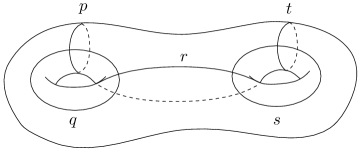
Figure 1: The Humphries generators for $\Sigma_{2}$.

As already mentioned, from the construction of the singular Jacobians one shows that singular fibers are of type $\text{I}_{1}\times T^{2}$, as we expect from the fact that all the monodromies that define $\mathcal{Y}_{1,1}$ are conjugate to the matrix $\mathbf{A}$ in (3.10). In fact, one can see that the list of monodromies (3.10) for $m=n=1$ defines a set of vanishing cycles for a genus-2 surface by noticing that in that case, all the matrices are elements of $Sp(4,\mathbb{Z})$, namely

$$\mathbf{A}^{t}\eta\mathbf{A}=\eta\,,\quad\mathbf{B}_{i}^{t}\eta\mathbf{B}_{i}=\eta\,,\quad\mathbf{C}_{i}^{t}\eta\mathbf{C}_{i}=\eta\,,$$ (3.130)

with

$$\eta=\begin{pmatrix}0&1&0&0\\ -1&0&0&0\\ 0&0&0&1\\ 0&0&-1&0\end{pmatrix}\,,$$ (3.131)

and they are all conjugate to $\mathbf{A}$ in $Sp(4,\mathbb{Z})$. Note that $Sp(4,\mathbb{Z})=\text{Aut}(H_{1}(\Sigma_{2};\mathbb{Z}))$ and from the surjective map

$$\Phi\,:\,MCG(\Sigma_{2})\rightarrow Sp(4,\mathbb{Z})\,,$$ (3.132)

we see that each monodromy represents an element of the mapping class group $MCG(\Sigma_{2})$, which is in fact a Dehn twist around a vanishing cycle of $\Sigma_{2}$. In this case, by a theorem of Humphries (see for example [24]), there is a minimum set of vanishing cycles such that their induced Dehn twists generate all the mapping class group. For a genus-2 surface these are shown in Figure 1. Picking the basis $(p,q,t,s)$, we see that the corresponding $Sp(4,\mathbb{Z})$ elements are

$$\mathbf{P}=\mathbf{A} =\begin{pmatrix}1&1&0&0\\ 0&1&0&0\\ 0&0&1&0\\ 0&0&0&1\end{pmatrix}\,,\quad\mathbf{Q}=\begin{pmatrix}1&0&0&0\\ -1&1&0&0\\ 0&0&1&0\\ 0&0&0&1\end{pmatrix}\,,\quad\mathbf{R}=\begin{pmatrix}1&1&0&-1\\ 0&1&0&0\\ 0&-1&1&1\\ 0&0&0&1\end{pmatrix}\,,$$ (3.133)

$$\mathbf{S} =\begin{pmatrix}1&0&0&0\\ 0&1&0&0\\ 0&0&1&0\\ 0&0&-1&1\end{pmatrix}\,,\quad\mathbf{T}=\begin{pmatrix}1&0&0&0\\ 0&1&0&0\\ 0&0&1&1\\ 0&0&0&1\end{pmatrix}\,.$$ (3.134)

A global model with trivial monodromy is obtained in this case from the known relation

$$\mathbf{H}^{2}=\mathbb{1}\,,$$ (3.135)

where $\mathbf{H}$ is an hyperelliptic involution, namely a $\pi$ rotation of $\Sigma_{2}$ around the horizontal axis in Figure 1. This is represented by the product

$$\mathbf{H}=\mathbf{T}\mathbf{S}\mathbf{R}\mathbf{Q}\mathbf{P}\mathbf{P}\mathbf{Q}\mathbf{R}\mathbf{S}\mathbf{T}\,.$$ (3.136)

The relation with the $\mathbf{A}$, $\mathbf{B}_{i}$, $\mathbf{C}_{i}$ monodromies arises from the appropriate braid relations and Hurwitz moves (see for example [9] for a review)

$$\mathbf{B}_{i}=\mathbf{T}_{i}\mathbf{Q}\mathbf{P}(\mathbf{T}_{i}\mathbf{Q})^{-1}\,,\quad\mathbf{C}_{i}=\mathbf{T}_{i}\mathbf{Q}^{-1}\mathbf{P}(\mathbf{T}_{i}\mathbf{Q}^{-1})^{-1}\,,$$ (3.137)

where

$$\mathbf{T}_{1}=\begin{pmatrix}1&0&0&-1\\ 0&1&0&0\\ 0&-1&1&0\\ 0&0&0&1\end{pmatrix}\,,\quad\mathbf{T}_{2}=\mathbb{1}\,,\quad\mathbf{T}_{3}=\begin{pmatrix}1&0&1&0\\ 0&1&0&0\\ 0&0&1&0\\ 0&-1&0&1\end{pmatrix}\,,\quad\mathbf{T}_{4}=\begin{pmatrix}1&0&1&-1\\ 0&1&0&0\\ 0&-1&1&0\\ 0&-1&0&1\end{pmatrix}\,.$$ (3.138)

4 $SL(2;\mathbb{Z})_{\tau}\times SL(2;\mathbb{Z})_{\rho}$ defects

The map between the T-duality group on a $T^{3}$ and the mapping class group of a $T^{4}$ can be used to construct a geometric model for the class of non-geometric backgrounds introduced in [2]. Such model is in fact obtained by lifting to M-theory the U-dual of the semi-flat limit of the latter solutions. The solutions of [2] are obtained by fibering the complex and Kähler moduli $(\tau,\rho)$ of a two-torus over a $\mathbb{P}^{1}$ base. If $\rho$ is fixed one recovers a semi-flat description of a K3 surface [25], while if also $\rho$ varies one obtains a non-geometric modification of the Calabi-Yau manifold. The metric of the non-trivial space-time directions is

$$ds^{2}=e^{\varphi}\tau_{2}\rho_{2}dzd\bar{z}+\frac{\rho_{2}}{\tau_{2}}\lvert dx+\tau dy\rvert^{2}$$ (4.1)

where $\tau=\tau_{1}+i\tau_{2}$, $\rho=\rho_{1}+i\rho_{2}$ and $\varphi$ are functions of $z$. At the generic smooth point in the moduli space, a K3 surface is described by a torus fibration with 24 singular points of type $\text{I}_{1}$. Locally these degenerations are described by compactified Taub-NUT spaces. In order to obtain a T-fold $\mathcal{X}$ we need to replace 12 $\text{I}_{1}$ degenerations with non-geometric defects determined by a monodromy in $\rho$. This corresponds to the factorizations

$$\mathbf{A}_{\tau}^{8}(\mathbf{B}_{\tau}\mathbf{C}_{\tau})^{2}=\mathbb{1}\,,\quad\mathbf{A}_{\rho}^{8}(\mathbf{B}_{\rho}\mathbf{C}_{\rho})^{2}=\mathbb{1}$$ (4.2)

where

$$\mathbf{A}=\begin{pmatrix}1&1\\ 0&1\end{pmatrix}\,,\quad\mathbf{B}=\begin{pmatrix}2&1\\ -1&0\end{pmatrix}\,,\quad\mathbf{C}=\begin{pmatrix}0&1\\ -1&2\end{pmatrix}$$ (4.3)

and the subscript refers to the two factors $SL(2;\mathbb{Z})_{\tau}\times SL(2;\mathbb{Z})_{\rho}$. It is slightly more useful to use two generators of $SL(2;\mathbb{Z})$: $\mathbf{U}=(\mathbf{A}^{-1})^{T}$, $\mathbf{V}=\mathbf{A}$, that corresponds to Dehn twists around the $(0,1)$ and $(1,0)$ cycles of the torus, respectively. The identity then simply factorises as $(\mathbf{U}\mathbf{V})^{6}=\mathbb{1}$. In order to switch to the $\mathbf{A}\mathbf{B}\mathbf{C}$ notation one uses the rules: $\mathbf{U}\mathbf{V}\mathbf{U}=\mathbf{V}\mathbf{U}\mathbf{V}$ and $\mathbf{U}\mathbf{V}^{n}=\mathbf{V}\mathbf{T}_{n}$ with $\mathbf{T}_{n+2}\mathbf{T}_{n}=\mathbf{B}\mathbf{C}$. For example we have

$$(\mathbf{U}\mathbf{V})^{6}=(\mathbf{V}\mathbf{U}\mathbf{V})^{4}=\mathbf{V}^{8}\mathbf{T}_{6}\mathbf{T}_{5}\mathbf{T}_{3}\mathbf{T}_{1}=\mathbf{A}^{8}(\mathbf{B}\mathbf{C})^{2}\,.$$ (4.4)

While the $\mathbf{A}_{\rho}$ monodromy should be associated with a NS5 brane [26], the $\mathbf{U}$ or $\mathbf{B}$, $\mathbf{C}$ monodromies involve a non-trivial action on the fiber volume, and this corresponds to a T-duality defect. The object with monodromy $\mathbf{U}_{\rho}$ is sometimes referred to as a $5_{2}^{2}$ or Q brane [27, 8, 28].

If we further compactify this setup on a spectator circle, we can apply the map between $O(3,3;\mathbb{Z})$ and $SL(4;\mathbb{Z})$ to construct a geometric dual model that involves a geometric $T^{4}$ fibration, in analogy with the examples discussed in the previous section. By setting $a=b=0$ in (A.13), (A.15) we see that we obtain a global factorization

$$\begin{diagram}$$ (4.5)

where the collections of $\tau$ and $\rho$ monodromies map to the data that specifies the fibration of the two $T^{2}$ factors and $M=12+12=24$. We see that the four type of elementary degenerations, corresponding to the type $\text{I}_{1}$ singularities, NS5 and non-geometric branes are mapped to the following $SL(4,\mathbb{Z})$ elements:

$$\mathbf{V}_{\tau}\mapsto\begin{pmatrix}\mathbf{V}&0\\ 0&\mathbb{1}\end{pmatrix}\,,\quad\mathbf{U}_{\tau}\mapsto\begin{pmatrix}\mathbf{U}&0\\ 0&\mathbb{1}\end{pmatrix}\,,\quad\mathbf{V}_{\rho}\mapsto\begin{pmatrix}\mathbb{1}&0\\ 0&\mathbf{V}\end{pmatrix}\,,\quad\mathbf{U}_{\rho}\mapsto\begin{pmatrix}\mathbb{1}&0\\ 0&\mathbf{U}\end{pmatrix}\,.$$ (4.6)

As in the fibrations constructed in section 3, locally each degeneration is of type $\text{I}_{1}\times T^{2}$, so the 5-branes are lifted to a Taub-NUT space. The global structure is however different. In the former case for $(m,n)=(0,0)$ one of the $T^{2}$ factors was trivially fibered and the total space was simply $\mathcal{Y}=K3\times T^{2}$.

Note that so far we considered T-folds whose geometric description is a smooth manifold $\mathcal{Y}$. We could consider singular points in the moduli space obtained by coalescing $\text{I}_{1}$ degenerations in $\mathcal{Y}$. This corresponds to coalesce some of the $\tau$ and $\rho$ degenerations. If we only collide $\tau$ or $\rho$ degenerations separately, the local description of the degeneration will be that of an ADE singularity in an appropriate duality frame. In particular, according to the Kodaira table, we can obtain all finite order elements in $SL(2,\mathbb{Z})$:

$$\text{II}\,:\,\mathbf{U}\mathbf{V}\,,\quad\text{III}\,:\,\mathbf{U}\mathbf{V}\mathbf{U}\,,\quad\text{IV}\,:\,(\mathbf{U}\mathbf{V})^{2}\,,\quad\text{I}_{0}^{\ast}\,:\,(\mathbf{U}\mathbf{V})^{3}\,,$$ (4.7)

$$\text{IV}^{\ast}\,:\,(\mathbf{U}\mathbf{V})^{4}\,,\quad\text{III}^{\ast}\,:\,(\mathbf{U}\mathbf{V})^{4}\mathbf{U}\,,\quad\text{II}^{\ast}\,:\,(\mathbf{U}\mathbf{V})^{5}\,,$$ (4.8)

as well as the parabolic elements $\text{I}_{k}\,:\,\,\mathbf{V}^{k}$, $\text{I}_{k}^{\ast}\,:\,\,(\mathbf{U}\mathbf{V})^{3}\mathbf{V}^{k}$. More interesting examples can be obtained by colliding a $\tau$ and a $\rho$ degeneration, similar to the examples in [9, 14]. For example, one can consider a defect of type $[\text{III},\text{III}]$ defined as

$$[\text{III},\text{III}]\,:\,\,\mathbf{U}_{\tau}\mathbf{V}_{\tau}\mathbf{U}_{\tau}\mathbf{U}_{\rho}\mathbf{V}_{\rho}\mathbf{U}_{\rho}\,.$$ (4.9)

In $\mathcal{Y}$, this corresponds to coalesce 6 $\text{I}_{1}$ mutually non-local singularities. This is superficially similar to the heterotic model studied in [14, 15], where a form of duality was found that, for example, relates a defect of type $[\text{III},\text{III}]$ with a geometric defect of type $\text{I}_{0}^{\ast}$. It would be interesting to see if a similar result applies to the present models.

4.1 Quantum corrected metrics

Both in the example considered in this and the previous sections, all the local monodromies around the duality defects are conjugate to a simple Dehn twist around one of the homology cycle of the torus, and in fact all the degenerations in the geometric spaces $\mathcal{Y}$ are of type $\text{I}_{1}\times T^{2}$. $\text{I}_{1}$ is the simplest type of degeneration in the Kodaira list and corresponds to pinching a cycle of the torus. This induces a monodromy that is a Dehn twist around the vanishing cycle. In a geometric space with no flux, a monodromy factorization such as (3.43) corresponds to a list of vanishing cycles for each degenerations. The situation is different for the spaces $\mathcal{X}$ where the B-field is non-trivial. The fact that all the monodromies are conjugate to a Dehn twist just means that we can apply Busher rules in the semi-flat approximation to exchange the B-field for a non-trivial twist in the metric. However, it is less clear how to extend such T-duality beyond the semi-flat approximation. What in the geometric description was a simple exchange of a vanishing cycle, is now a T-duality in the full string theory, relating the $\text{I}_{1}$ singularity with a 5-brane. In order to describe the local setting, we can neglect the extra circle of the $T^{3}$ and just consider a $T^{2}$ fibration on a disk encircling the defect. We can take the monodromy of the torus to be, as in (4.3)

$$\mathbf{V}=\begin{pmatrix}1&1\\ 0&1\end{pmatrix}\,,$$ (4.10)

which acts as $\tau\rightarrow\tau+1$ on the complex structure of the torus. The semi-flat local metric is simply a foliation of the bundle (2.12) and it is given by (4.1) with $\rho=0$ and $\tau=\frac{i}{2\pi}\log(\mu/z)$. The exact metric can be found by compactifying a Taub-NUT space on the $(0,1)$ cycle of the torus, and identifying the shrinking $(1,0)$ cycle with the special circle. This results in the Ooguri-Vafa metric [29]

$$ds^{2}=H(dr^{2}+r^{2}d\theta^{2}+dx^{2})+\frac{1}{H}(dy+\omega)^{2}$$ (4.11)

with

$$H=\frac{1}{2\pi}\log(\mu/r)+\sum_{n\neq 0}e^{inx}K_{0}\left(|n|r\right)\,,$$ (4.12)

where we set the radii to 1 and $K_{0}$ is the modified Bessel function of the second kind. The non-perturbative corrections in (4.12) localizes the shrinking cycle along the orthogonal one and breaks one of the $U(1)^{2}$ isometries of the semi-flat metric. On the other hand, the action of the monodromy $\mathbf{V}$ on the Kähler modulus, i.e. $\rho\rightarrow\rho+1$ represents a defect that should be identified with a NS5 brane [26, 30]. The exact metric clearly breaks both the $U(1)^{2}$ isometries of the semi-flat solution. In fact after Poisson resummation the harmonic function can be written as

$$H=\frac{1}{2\pi}\log(\mu/r)+\frac{1}{2\pi}\sum_{k_{x},k_{y}\in\mathbb{Z}\setminus\{0\}}K_{0}(\lambda r)e^{-ik_{x}x-ik_{y}y}\,,$$ (4.13)

with $\lambda=\sqrt{k_{x}^{2}+k_{y}^{2}}$. Hence, by realizing $\rho$ monodromies as geometric $\text{I}_{1}$ singularities, we are missing part of the modes that fully describe the exact metrics beyond the semi-flat approximation. Similarly, one can consider the non-geometric monodromies which are $\beta$ transformations in the duality group. For the $T^{2}$ example, this is just a monodromy $\mathbf{U}_{\rho}$. Lacking a worldsheet description of such object we do not know what is the exact form of the corrected non-geometric solution. One can give the following argument, which is essentially a semi-flat version of [31]. The monodromy $\mathbf{V}_{\rho}$ results in the non-conservation of momentum along the fiber directions. This is compensated by an inflow of current where there is a change in the kinetic terms of the zero modes for translations along the fiber directions $(x\rightarrow x+\alpha_{x}\,,y\rightarrow y+\alpha_{y})$. Note that $\mathbf{V}_{\rho}$ does not act on the lattice of windings for strings on the torus. On the other hand, the duality to a non-geometric monodromy $\mathbf{U}_{\rho}$ results in a trivial action on the lattice of momenta, but it leads to non-conservation of the winding numbers $(w_{x},w_{y})$. The effective dynamics should then involve couplings between the winding modes and “dyonic” degrees of freedom whose kinetic term is increased as the winding charge decreases by encircling the defect. This would result in an expression for string winding fields that involves Fourier modes similar to (4.13), with the dyonic modes identified with the dual of the zero modes $(\alpha_{x}\,,\alpha_{y})$. This structure is not visible in supergravity in the non-geometric duality frame, and it is presumably accessed by correlation functions in the winding sector. We expect this argument to give a qualitatively correct picture in a regime where the Bessel function in (4.13) is well approximated by exponential decaying terms. Close to the origin, at least for a stack of defects, one should recover the 5-branes linear dilaton throat.

It is interesting to note that a similar situation arises in the F-theory models of [11, 14, 15] that are dual to non-geometric background of the heterotic theory. In that case, if one describes defects with monodromy in $\tau$ and $\rho$ by two elliptic fibrations

$$y^{2}=x^{3}+f_{\tau}(z)x+g_{\tau}(z)\,,\quad y^{2}=x^{3}+f_{\rho}(z)x+g_{\rho}(z)\,,$$ (4.14)

with $z$ a complex coordinate in the neighborhood of the degeneration, there exists a map to a dual K3 fibered Calabi-Yau threefold descending from an adiabatic fibration of 8 dimensional heterotic/F-theory duality on a common base:

$$y^{2}=x^{3}-3f_{\tau}(z)f_{\rho}(z)xu^{4}+\frac{\Delta_{\tau}(z)\Delta_{\rho}(z)}{16}u^{5}-\frac{27}{2}g_{\tau}(z)g_{\rho}(z)+u^{7}\,,$$ (4.15)

where $\Delta=4f^{3}+27g^{2}$ is the discriminant of the Weierstraß  equations, and $u$ is a complex coordinate on a $\mathbb{P}^{1}$ base. Local models of $\text{I}_{k}$ singularities, NS5 branes and non-geometric $\mathbf{U}_{\rho}$ defects are all dualized to the same local geometric model since the map (4.15) is symmetric in $\tau$ and $\rho$, as expected from T-duality. The discussion above implies a particular form of corrections to the adiabatic approximation. It would be interesting to check this for NS5 branes, keeping track of their position on the fiber through the duality.

Acknowledgments

We are grateful to Valentí Vall Camell for useful discussions. This work was partially supported by the ERC Advanced Grant “Strings and Gravity” (Grant. No. 320045) and by the DFG cluster of excellence “Origin and Structure of the Universe”. The work of SM is supported in part by DOE grant DE-SC0009924.

Appendix A The map from $SL(4)$ to $SO(3,3)^{+}$

We construct the homomorphism of Lie groups

$$SL(4;\mathbb{R})\rightarrow SO(3,3;\mathbb{R})^{+}$$ (A.1)

which is a double cover, implying $SL(4;\mathbb{R})\cong Spin(3,3;\mathbb{R})$. We first pick a basis

$$\mathbb{R}^{4}=\langle e_{1},...,e_{4}\rangle$$ (A.2)

which induces a basis of $\Lambda^{2}\mathbb{R}^{4}$ given by

$$\{e_{23},-e_{13},e_{12},e_{14},e_{24},e_{34}\},$$ (A.3)

where $e_{ij}=e_{i}\wedge e_{j}$. We define the scalar product on $\Lambda^{2}\mathbb{R}^{4}$ by

$$\langle x,y\rangle e_{1}\wedge...\wedge e_{4}=x\wedge y,$$ (A.4)

for $x,y\in\Lambda^{2}\mathbb{R}^{4}$. Now let $A\in SL(4;\mathbb{R})$ act on $\mathbb{R}^{4}$ by left multiplication. We view elements of $\mathbb{R}^{4}$ as column vectors. Then there is an induced action of $SL(4;\mathbb{R})$ on $\Lambda^{2}\mathbb{R}^{4}$ given by

$$A\cdot(e_{i}\wedge e_{j})=(Ae_{i})\wedge(Ae_{j}).$$ (A.5)

Because of the well-known identity

$$(Ae_{1})\wedge(Ae_{2})\wedge(Ae_{3})\wedge(Ae_{4})=\text{Det}(A)e_{1}\wedge...\wedge e_{4}=e_{1}\wedge...\wedge e_{4},$$ (A.6)

this action leaves the scalar product on $\Lambda^{2}\mathbb{R}^{4}$ invariant. We therefore expand

$$A\cdot e_{ij}=\sum_{kl}B_{ij,kl}e_{kl},$$ (A.7)

and obtain a $6\times 6$ matrix $B$, which acts on $\Lambda^{2}\mathbb{R}^{4}$ by left multiplication where we view elements of $\Lambda^{2}{\mathbb{R}}^{4}$ as column vectors with respect to the basis above. By construction this matrix leaves the scalar product invariant. But explicitly we calculate

$$\langle e_{14},e_{23}\rangle=1\ \ \ \langle e_{24},-e_{13}\rangle=1\ \ \ \langle e_{34},e_{12}\rangle=1,$$ (A.8)

with all other combinations of basis vectors having vanishing scalar product. In matrix form the scalar product is given by

$$\eta=\left(\begin{array}[]{ccc|ccc}0&0&0&1&0&0\\ 0&0&0&0&1&0\\ 0&0&0&0&0&1\\ \hline\cr 1&0&0&0&0&0\\ 0&1&0&0&0&0\\ 0&0&1&0&0&0\end{array}\right)\,.$$ (A.9)

As mentioned above by construction

$$B^{T}\eta B=\eta,$$ (A.10)

thus $B\in SO(3,3;\mathbb{R})$. Now one checks explicitly that

$$\left(\begin{array}[]{c|c}R&\\ \hline\cr&1\end{array}\right)\in SL(4;\mathbb{R})\,,$$ (A.11)

with $R\in SL(3;\mathbb{R})$ is mapped to the diffeomorphism

$$\left(\begin{array}[]{c|c}(R^{-1})^{T}&0\\ \hline\cr 0&R\end{array}\right)\in O(3,3;\mathbb{R})\,.$$ (A.12)

The element

$$\left(\begin{array}[]{ccc|c}1&0&0&a\\ 0&1&0&b\\ 0&0&1&c\\ \hline\cr 0&0&0&1\\ \end{array}\right)$$ (A.13)

maps to

$$\left(\begin{array}[]{c|c}\mathbb{1}&\omega\\ \hline\cr 0&\mathbb{1}\end{array}\right)\,,$$ (A.14)

with

$$\omega=\left(\begin{array}[]{ccc}0&c&-b\\ -c&0&a\\ b&-a&0\end{array}\right)\,,$$ (A.15)

which is a gauge transformation for the B-field. Similarly,

$$\left(\begin{array}[]{ccc|c}1&0&0&0\\ 0&1&0&0\\ 0&0&1&0\\ \hline\cr a&b&c&1\\ \end{array}\right)$$ (A.16)

is mapped to a $\beta$-transformation

$$\left(\begin{array}[]{c|c}\mathbb{1}&0\\ \hline\cr-\omega&\mathbb{1}\end{array}\right)\,.$$ (A.17)

Appendix B SYZ fibrations

The extension of our results to the case of a three dimensional base, e.g. $S^{3}$ are challenging since in this case both local and global aspects are much less understood, even for the geometric case of SYZ fibrations. Some non-geometric generalizations corresponding to asymmetric orbifold points have been considered in [4]. A possibility is that the local structure around the discriminant locus of a $T^{3}$ fibrations is modified to account for non-geometric monodromies. Remember that the quintic viewed as the total space of a $T^{3}$ fibration has discriminant locus a trivalent graph $\Gamma$ embedded in $S^{3}$ (see for instance [35] for a review). The monodromy around the edges of $\Gamma$ is in the same conjugacy class of the matrices in (2.11) and the monodromies around a vertex have the following representatives (see Figure 2):

• Positive vertex

  $$T_{1+}=\begin{pmatrix}1&0&1\\ 0&1&0\\ 0&0&1\end{pmatrix}\,,\quad T_{2+}=\begin{pmatrix}1&0&0\\ 0&1&1\\ 0&0&1\end{pmatrix}\,,\quad T_{3+}=T_{2+}^{-1}T_{1+}^{-1}=\begin{pmatrix}1&0&-1\\ 0&1&-1\\ 0&0&1\end{pmatrix}\,,$$ (B.1)

• Negative vertex

  $$T_{1-}=\begin{pmatrix}1&0&1\\ 0&1&0\\ 0&0&1\end{pmatrix}\,,\quad T_{2-}=\begin{pmatrix}1&1&0\\ 0&1&0\\ 0&0&1\end{pmatrix}\,,\quad T_{3-}=T_{2-}^{-1}T_{1-}^{-1}=\begin{pmatrix}1&-1&-1\\ 0&1&0\\ 0&0&1\end{pmatrix}\,.$$ (B.2)

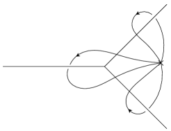
Figure 2: Monodromies around a vertex.

Since all the monodromies are conjugate to the ones in (2.11), it might be possible to extend the conjugacy class in the duality group, and use the more general monodromies in $O(3,3,\mathbb{Z})$ of section (3.2). As a first step in this direction, one would like to understand the analogous of the semi-flat metric (4.1) for $T^{3}$. We will adapt an approach that was used in [6] to study non-perturbative defects with monodromies in the U-duality group $SL(3,\mathbb{Z})$. Identifying the duality group with the group of large diffeomorphisms of a $T^{3}$ this leads to the study of $T^{3}$ fibered CY three-folds. One start with the following semi-flat ansatz

$$ds^{2}=e^{2\phi_{1}}dx_{1}^{2}+e^{2\phi_{2}}dx_{2}^{2}+e^{2\phi_{3}}dx_{3}^{3}+G_{ij}dy^{i}dy^{j}\,,\quad G=V^{T}V$$ (B.3)

with $V$ given by

$$V=e^{-\frac{2\alpha_{1}+\alpha_{2}}{3}}\left(\begin{array}[]{ccc}1&a&b\\ 0&e^{-\alpha_{1}}&e^{-\alpha_{1}}c\\ 0&0&e^{-\alpha_{1}-\alpha_{2}}\end{array}\right).$$ (B.4)

All the scalars (B.3) are functions of the $\mathbb{R}^{3}$ base coordinates $x_{i}$. We indicate by $y_{i}$ the coordinates on the $T^{3}$. The prescription of [6] is to pick a complex structure by pairing base and fiber coordinates as follows. We use the differential forms $dz^{i}=e^{\phi_{i}}dx^{i}+i\delta_{ij}V_{jk}dy^{k}$, explicitly:

$$dz^{1} =e^{\phi_{1}}dx_{1}+ie^{\frac{1}{3}(2\alpha_{1}+\alpha_{2})}(dy_{1}+a\,dy_{2}+b\,dy_{3})\,,$$ (B.5)

$$dz^{2} =e^{\phi_{2}}dx_{2}+ie^{\frac{1}{3}(-\alpha_{1}+\alpha_{2})}(dy_{2}+c\,dy_{3})\,,$$

$$dz^{3} =e^{\phi_{3}}dx_{3}+ie^{-\frac{1}{3}(\alpha_{1}+2\alpha_{2})}(dy_{3})\,,$$

and we write

$$J=e^{\phi_{i}}V_{ij}dx^{i}\wedge dy^{j}\,,\quad\Omega=idz^{1}\wedge dz^{2}\wedge dz^{3}\,.$$ (B.6)

We then see that requiring $d\Omega=dJ=0$ is equivalent to the following system of 15 PDEs for the metric moduli:

$$\partial_{1}a =e^{-\alpha_{1}+\phi_{1}-\phi_{2}}\partial_{2}(\alpha_{1}-\phi_{3})\,,\quad\partial_{2}a=2e^{-\alpha_{1}-\phi_{1}+\phi_{2}}\partial_{1}\phi_{2}\,,\quad\partial_{3}a=0\,,$$ (B.7)

$$\partial_{1}b =-2e^{-\alpha_{1}-\alpha_{2}+\phi_{1}-\phi_{3}}\partial_{3}\phi_{1}+c\partial_{1}a\,,\quad\partial_{2}b=c\partial_{2}a\,,\quad\partial_{3}b=2e^{-\alpha_{1}-\alpha_{2}-\phi_{1}+\phi_{3}}\partial_{1}\phi_{3}\,,$$

$$\partial_{1}c =0\,,\quad\partial_{2}c=-2e^{-\alpha_{2}+\phi_{2}-\phi_{3}}\partial_{3}\phi_{2}\,,\quad\partial_{3}c=2e^{-\alpha_{2}-\phi_{2}+\phi_{3}}\partial_{2}\phi_{3}\,,$$

$$\partial_{2}\phi_{1} =-\frac{1}{3}\partial_{2}(2\alpha_{1}+\alpha_{2})\,,\qquad\partial_{3}\phi_{1}=-\frac{1}{3}\partial_{3}(2\alpha_{1}+\alpha_{2})\,,$$

$$\partial_{1}\phi_{2} =\frac{1}{3}\partial_{1}(-\alpha_{1}+\alpha_{2})\,,\qquad\partial_{3}\phi_{2}=\frac{1}{3}\partial_{3}(\alpha_{1}-\alpha_{2})\,,$$

$$\partial_{1}\phi_{3} =\frac{1}{3}\partial_{1}(-\alpha_{1}-2\alpha_{2})\,,\qquad\partial_{2}\phi_{3}=-\frac{1}{3}\partial_{2}(\alpha_{1}+2\alpha_{2})\,.$$

By setting for instance $b=c=0$ we can describe the embedding of a $T^{2}$ with complex structure $\tau=a+ie^{-\alpha_{1}}$, and this should be relevant for the monodromy (2.11). In this limit the fields do not depend on $x_{3}$, and $\phi_{3}$ is a constant. If we take $\phi_{1}=\phi_{2}$ we then get, fixing an integration constant:

$$\phi_{1}=\phi_{2}=\alpha_{2}=-\alpha_{1}/2\,,\quad\partial_{1}a=-\partial_{2}e^{-\alpha_{1}}\,,\quad\partial_{2}a=\partial_{1}e^{-\alpha_{1}}\,,$$ (B.8)

the last two equations giving the Cauchy-Riemann equation for $\tau=a+ie^{-\alpha_{1}}$ with complex coordinate $z=x_{1}+ix_{2}$. The metric (B.3) takes the form

$$ds^{2}=dx_{3}^{2}+dy_{3}^{2}+e^{-\alpha_{1}}dzd\bar{z}+G_{ij}dy^{i}dy^{j}\,,\quad i,j=1,2\,,$$ (B.9)

with

$$G=e^{\alpha_{1}}\begin{pmatrix}1&a\\ a&e^{-2\alpha_{1}}+a^{2}\end{pmatrix}\,.$$ (B.10)

This is the semi-flat metric (4.1), with $\rho=0$, where the conformal factor $\varphi$ has been set to zero. This reproduces the leading order Ooguri-Vafa metric (4.11) for which

$$\tau=\frac{i}{2\pi}\log\left(\frac{\mu}{z}\right)\,,\quad e^{\varphi}=1\,.$$ (B.11)

The monodromy is $\tau\rightarrow\tau+1$, corresponding to action of the matrix $\mathbf{V}$ in (4.10) on $\tau$. However, we cannot embed a solution for the general conjugacy class of $\mathbf{V}$, which is parametrized by integers $(p,q)$, since in general this requires a non-zero $\varphi$. By including the $\rho$ modulus, one encounter the same situation. The semi-flat approximation of the NS5 brane has $\rho=i/(2\pi)\log(\mu/z)$ and $e^{\varphi}=1$. The solution for the non-geometric defect with monodromy $\mathbf{U}$ is given instead by

$$\rho=\frac{2\pi i}{\log\left(\frac{\mu}{z}\right)}\,,\quad e^{\varphi}=i\sigma\log\left(\frac{\mu}{z}\right)\,.$$ (B.12)

So while we can obtain the correct metric on the fiber, some more work is needed to write fully non-geometric solutions using this approach. We defer a detailed analysis to future work.

References

- [1] A. Strominger, S.-T. Yau, and E. Zaslow, “Mirror symmetry is T duality,” Nucl.Phys. B479 (1996) 243–259, arXiv:hep-th/9606040 [hep-th].
- [2] S. Hellerman, J. McGreevy, and B. Williams, “Geometric constructions of nongeometric string theories,” JHEP 0401 (2004) 024, arXiv:hep-th/0208174 [hep-th].
- [3] C. Hull, “A Geometry for non-geometric string backgrounds,” JHEP 0510 (2005) 065, arXiv:hep-th/0406102 [hep-th].
- [4] D. Vegh and J. McGreevy, “Semi-Flatland,” JHEP 0810 (2008) 068, arXiv:0808.1569 [hep-th].
- [5] A. Kumar and C. Vafa, “U manifolds,” Phys.Lett. B396 (1997) 85–90, arXiv:hep-th/9611007 [hep-th].
- [6] J. T. Liu and R. Minasian, “U-branes and T**3 fibrations,” Nucl.Phys. B510 (1998) 538–554, arXiv:hep-th/9707125 [hep-th].
- [7] L. Martucci, J. F. Morales, and D. R. Pacifici, “Branes, U-folds and hyperelliptic fibrations,” JHEP 1301 (2013) 145, arXiv:1207.6120 [hep-th].
- [8] J. de Boer and M. Shigemori, “Exotic Branes in String Theory,” Phys.Rept. 532 (2013) 65–118, arXiv:1209.6056 [hep-th].
- [9] D. Lüst, S. Massai, and V. Vall Camell, “The monodromy of T-folds and T-fects,” JHEP 09 (2016) 127, arXiv:1508.01193 [hep-th].
- [10] C. Vafa, “Evidence for F theory,” Nucl.Phys. B469 (1996) 403–418, arXiv:hep-th/9602022 [hep-th].
- [11] J. McOrist, D. R. Morrison, and S. Sethi, “Geometries, Non-Geometries, and Fluxes,” Adv.Theor.Math.Phys. 14 (2010) , arXiv:1004.5447 [hep-th].
- [12] A. Malmendier and D. R. Morrison, “K3 surfaces, modular forms, and non-geometric heterotic compactifications,” Lett. Math. Phys. 105 no. 8, (2015) 1085–1118, arXiv:1406.4873 [hep-th].
- [13] I. García-Etxebarria, D. Lüst, S. Massai, and C. Mayrhofer, “Ubiquity of non-geometry in heterotic compactifications,” JHEP 03 (2017) 046, arXiv:1611.10291 [hep-th].
- [14] A. Font, I. García-Etxebarria, D. Lüst, S. Massai, and C. Mayrhofer, “Heterotic T-fects, 6D SCFTs, and F-Theory,” JHEP 08 (2016) 175, arXiv:1603.09361 [hep-th].
- [15] A. Font and C. Mayrhofer, “Non-geometric vacua of the heterotic string and little string theories,” JHEP 11 (2017) 064, arXiv:1708.05428 [hep-th].
- [16] A. Giveon, M. Porrati, and E. Rabinovici, “Target space duality in string theory,” Phys.Rept. 244 (1994) 77–202, arXiv:hep-th/9401139 [hep-th].
- [17] C. Bock, “On Low-Dimensional Solvmanifolds,” ArXiv e-prints (Mar., 2009) , arXiv:0903.2926 [math.DG].
- [18] R. Donagi, P. Gao, and M. B. Schulz, “Abelian Fibrations, String Junctions, and Flux/Geometry Duality,” JHEP 04 (2009) 119, arXiv:0810.5195 [hep-th].
- [19] M. B. Schulz, “Calabi-Yau duals of torus orientifolds,” JHEP 05 (2006) 023, arXiv:hep-th/0412270 [hep-th].
- [20] Y. Namikawa and K. Ueno, “The complete classification of fibres in pencils of curves of genus two,” Manuscripta Math. 9 no. 2, (1973) 143–186. http://dx.doi.org/10.1007/BF01297652.
- [21] A. B. Altman and S. L. Kleiman, The presentation functor and the compactified Jacobian, pp. 15–32. Birkhäuser Boston, Boston, MA, 2007. http://dx.doi.org/10.1007/978-0-8176-4574-8_2.
- [22] J. Kass, “Notes on compactified jacobian,” 2008. http://people.math.sc.edu/kassj/Lecture%20Notes%20on%20Compactified%20Jacobians.pdf.
- [23] R. Gompf and A. Stipsicz, 4-manifolds and Kirby Calculus. Graduate studies in mathematics. American Mathematical Society, 1999. https://books.google.de/books?id=ahLKzRUTBbUC.
- [24] B. Farb and D. Margalit, A Primer on Mapping Class Groups. Princeton University Press, 2011.
- [25] B. R. Greene, A. D. Shapere, C. Vafa, and S.-T. Yau, “Stringy Cosmic Strings and Noncompact Calabi-Yau Manifolds,” Nucl.Phys. B337 (1990) 1.
- [26] H. Ooguri and C. Vafa, “Two-dimensional black hole and singularities of CY manifolds,” Nucl.Phys. B463 (1996) 55–72, arXiv:hep-th/9511164 [hep-th].
- [27] N. Obers and B. Pioline, “U duality and M theory,” Phys.Rept. 318 (1999) 113–225, arXiv:hep-th/9809039 [hep-th].
- [28] F. Hassler and D. Lüst, “Non-commutative/non-associative IIA (IIB) Q- and R-branes and their intersections,” JHEP 1307 (2013) 048, arXiv:1303.1413 [hep-th].
- [29] H. Ooguri and C. Vafa, “Summing up D instantons,” Phys.Rev.Lett. 77 (1996) 3296–3298, arXiv:hep-th/9608079 [hep-th].
- [30] K. Becker and S. Sethi, “Torsional Heterotic Geometries,” Nucl.Phys. B820 (2009) 1–31, arXiv:0903.3769 [hep-th].
- [31] R. Gregory, J. A. Harvey, and G. W. Moore, “Unwinding strings and t duality of Kaluza-Klein and h monopoles,” Adv.Theor.Math.Phys. 1 (1997) 283–297, arXiv:hep-th/9708086 [hep-th].
- [32] J. A. Harvey and S. Jensen, “Worldsheet instanton corrections to the Kaluza-Klein monopole,” JHEP 10 (2005) 028, arXiv:hep-th/0507204 [hep-th].
- [33] D. Lüst, E. Plauschinn, and V. Vall Camell, “Unwinding strings in semi-flatland,” JHEP 07 (2017) 027, arXiv:1706.00835 [hep-th].
- [34] A. Giveon and D. Kutasov, “Little string theory in a double scaling limit,” JHEP 10 (1999) 034, arXiv:hep-th/9909110 [hep-th].
- [35] D. R. Morrison, “On the structure of supersymmetric T3 fibrations,” ArXiv e-prints (Feb., 2010) , arXiv:1002.4921 [math.AG].