Detecting metal-poor gas accretion in the star-forming dwarf galaxies UM 461 and Mrk 600

Abstract

Using VIMOS-IFU observations, we study the interstellar medium (ISM) of two star-forming dwarf galaxies, UM 461 and Mrk 600. Our aim was to search for the existence of metallicity inhomogeneities that might arise from infall of nearly pristine gas feeding ongoing localized star-formation. The IFU data allowed us to study the impact of external gas accretion on the chemical evolution as well as the ionised gas kinematics and morphologies of these galaxies. Both systems show signs of morphological distortions, including cometary-like morphologies. We analysed the spatial variation of 12 + log(O/H) abundances within both galaxies using the direct method (T_e), the widely applied HII–CHI–mistry code, as well as by employing different standard calibrations. For UM 461 our results show that the ISM is fairly well mixed, at large scales, however we find an off-centre and low-metallicity region with 12 + log(O/H) $<$ 7.6 in the SW part of the brightest H ii region, using the direct method. This result is consistent with the recent infall of a low mass metal-poor dwarf or H i cloud into the region now exhibiting the lowest metallicity, which also displays localized perturbed neutral and ionized gas kinematics. Mrk 600 in contrast, appears to be chemically homogeneous on both large and small scales. The intrinsic differences in the spatially resolved properties of the ISM in our analysed galaxies are consistent with these systems being at different evolutionary stages.

1 Introduction

The structure of the starbursting regions and underlying stellar component of star-forming dwarf galaxies can provide significant information on the mechanical energy input from and photoionization by the newly born stars. The distribution of these regions across a galaxy can also provide information on the effect of external interactions or mergers. The morphology currently displayed by a dwarf galaxy could have arisen via several alternative evolutionary pathways (e.g. Tolstoy, Hill & Tosi, 2009). In particular, star-forming dwarf galaxies with cometary morphology are commonly observed in high-redshift surveys, such as the Hubble Deep Field (HDF; e.g. van den Bergh et al., 1996; Straughn et al., 2006; Windhorst et al., 2006). This cometary morphology has been interpreted for high redshift galaxies in the HDF as: 1) the result of weak tidal interactions; 2) gravitational instabilities in gas-rich and turbulent galactic disks in the process of forming (Bournaud & Elmegreen, 2009) and 3) stream-like accretion of metal-poor gas from the cosmic web (e.g. Dekel & Birnboim, 2006; Dekel et al., 2009). Interestingly, at low redshift, a significant fraction of low-mass ($\sim$10⁸–10⁹M_⊙), low-luminosity (10⁷ $\lesssim$ L/L${}_{\odot}\lesssim$ 10⁹) and low-metallicity (Z_⊙/40 $\lesssim$ Z $\lesssim$ Z_⊙/3) H ii or blue compact dwarf (BCD) galaxies also have cometary or elongated stellar morphologies (Papaderos et al., 2008).

The study of star-formation feedback and the role played by galaxy interactions in low redshift dwarfs may offer important insights into galaxy evolution processes in the young Universe. Recently, some studies (e.g. Sánchez Almeida et al., 2014, 2015) highlighted the existence of spatially resolved chemical inhomogeneities in the ISM of some local H ii/BCDs and extremely metal-poor (XMP) BCD galaxies, which possibly originated from the accretion of nearly pristine cold gas. The same mechanism has been invoked by Cresci et al. (2010) to interpret the radial metallicity gradient of massive z $\sim$ 3 galaxies as evidence of accretion of primordial gas, which in turn is sustaining the high star-formation activity predicted by cold flow models. Sánchez Almeida et al. (2015) interpret their result, in the case of nearby XMP BCDs, as arising from gas-cloud infall from the cosmic web. However, if we use the oxygen abundance (12 + log(O/H)) as a spatially resolved metallicity tracer, most of the H ii/BCD (e.g. Lagos et al., 2009, 2012) and XMP (e.g. Lagos et al., 2014, 2016; Kehrig et al., 2016) galaxies studied so far turn out to be chemically homogeneous at large scales ($\sim$0.5 - 1 kpc). This suggest the presence of global hydro-dynamical effects being responsible for efficient gas transport and mixing across the galaxies (e.g. Lagos & Papaderos, 2013, and references therein). Also, the N/O ratio in most of these galaxies has been found to be homogeneous within the uncertainties. Even so, the slight anti-correlation between star-formation and metallicity in the cometary galaxy Tol 65 (Lagos et al., 2016) indicates that the infall/accretion of metal-poor gas or minor merger/interactions, in the recent past, may have produced its moderate abundance gradient and cometary stellar morphology. In this sense, Olmo-García et al. (2017) argue that if the accretion of metal-poor gas is fueling the star-formation the metallicity (O/H) of the pre-enriched gas is reduced but it cannot modify the pre-existing ratio between the metals, then keeping the N/O ratio constant across the ISM.

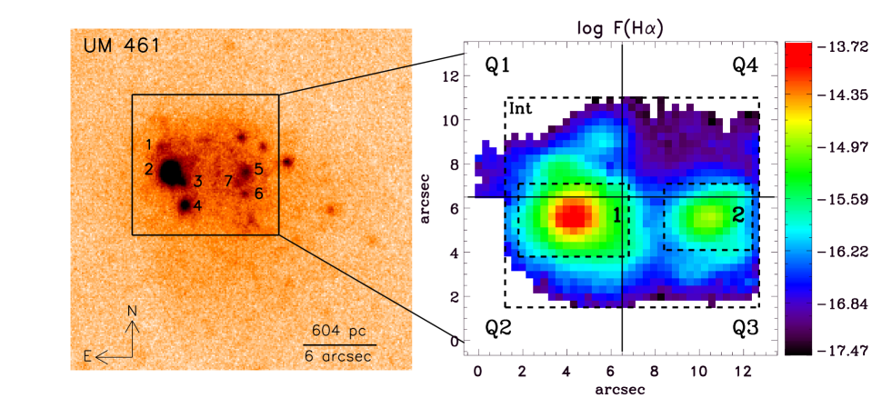
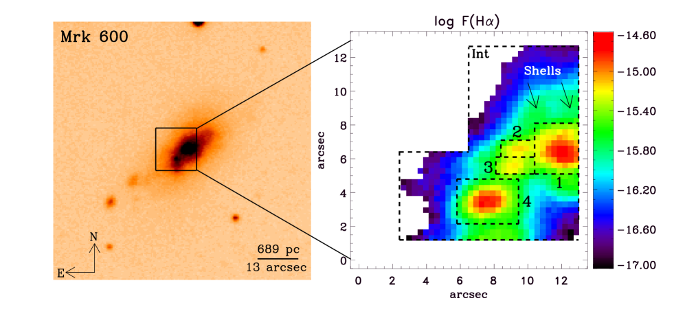
Figure 1: UM 461 and Mrk 600 optical/NIR images (left) and VIMOS H${\alpha}$ maps (right). Top left: UM 461, K_p band image (Lagos et al., 2011). The numbers on image show the positions of star clusters identified in Lagos et al. (2011) using the notation from that paper. Bottom left: Mrk 600, R band image (Gil de Paz, Madore & Pevunova, 2003). Right : H$\alpha$ emission line flux (logarithmic scale) maps for the VIMOS-IFU 13″$\times$13 ″FoV for each galaxy. The dotted black lines on the images indicate the apertures used in our analysis; regions 1–2 for UM 461, 1–4 in Mrk 600 and the integrated (Int) ones. For the UM 461 map the VIMOS CCD quadrants (Q1$\ldots$Q4) are overlaid on image. Further details are given in Section 2. The H$\alpha$ fluxes are in units of ergs cm^-2 s^-1.

Here we present new Very Large Telescope (VLT) VIsible MultiObject Spectrograph (VIMOS; Le Févre et al., 2003) observations of two star-forming dwarf galaxies using the integral field unit (IFU) spectroscopy mode (hereafter VIMOS-IFU). UM 461 (upper panel in Figure 1) is a well studied H ii/BCD galaxy (e.g. Taylor et al., 1995; van Zee, Skillman & Salzer, 1998; Lagos et al., 2011). This galaxy has been described as formed by two compact and off-centre giant H ii  regions (GH iiR), some smaller star-forming regions spread across the galaxy disk and an external stellar envelope that is strongly skewed towards the south-west (Lagos et al., 2011). It has been classified as having a cometary-like morphology with an integrated subsolar metallicity of 12 + log(O/H) = 7.73 - 7.78 (Masegosa, Moles & Campos-Aguilar, 1994; Izotov & Thuan, 1998; Pérez-Montero & Díaz, 2003). As in most H ii/BCD galaxies, UM 461 has an underlying component of old stars (Telles & Terlevich, 1997; Lagos et al., 2011) that exhibits an elliptical outer morphology. Deep Near-Infrared observations with the Gemini/NIRI camera (Lagos et al., 2011) revealed that the star-formation activity in this galaxy is taking place in several star clusters with masses typically between $\sim$10⁴ M_⊙ and $\sim$10⁶ M_⊙. Figure 1 shows the K_p band image of UM 461 obtained by Lagos et al. (2011). Using the same notation as Lagos et al. (2011), the main GH iiR (the brightest one in Figure 1) in our study is composed of the star clusters no. 2 and no. 3, while the faintest one is formed by star clusters no. 5, no. 6 and no. 7. Taylor et al. (1995) proposed that the SE tail in their H i  image of  UM 461 was formed as a result of a tidal interaction with UM 462. However, higher resolution H i maps of UM 461 by van Zee, Skillman & Salzer (1998) did not show the extended SE H i tail seen in the Taylor H i map. This discrepancy is attributed to solar interference in the Taylor map (van Zee, Skillman & Salzer, 1998). Moreover, the age distribution of the star cluster population in UM 461 indicates that the current star burst has began within the last few million years (Lagos et al., 2011). This current star burst time scale is too short to realistically be attributed to a UM 461/UM 462 interaction.

Mrk 600 (lower panel in Figure 1) was classified as an iE BCD according to the Loose & Thuan (1986) classification scheme. However, the elongated shape and the presence of several fainter regions beyond the main body of the galaxy indicate a tadpole or cometary-like stellar morphology. The ongoing star-forming activity in this object (see Cairós et al., 2001a) is mainly concentrated in the two principal GH iiRs. Spatially resolved colours of those regions (Cairós et al., 2001b) are consistent with a young starburst. The distribution of these H ii regions may be the result of a recent interaction given the presence of a nearby H i companion (Taylor, Brinks & Skillman, 1993) as suggested by Noeske et al. (2005). Izotov & Thuan (1998) and Guseva et al. (2011) derived an integrated oxygen abundance of 12 + log(O/H) = 7.83 - 7.88 for Mrk 600. Basic properties for both galaxies are compiled in Table 1.

Table 1: Basic properties of UM 461 and Mrk 600.

Parameter	Value	Reference
UM 461
RA (J2000)	11h51m33.3s	Obtained from NED
DEC (J2000)	-02o22m22s	Obtained from NED
Distance (3K CMB) Mpc	19.2	Obtained from NED
Pixel scale (pc/arcsec)	93	Obtained from NED
z	0.003465	Obtained from NED
E(B-V)Gal mag	0.014	Schlafly & Finkbeiner (2011)
c(H$\beta$)	0.12	Izotov & Thuan (1998)
12 + log(O/H)	7.73$\pm$0.03, 7.78$\pm$0.03	Masegosa, Moles & Campos-Aguilar (1994); Izotov & Thuan (1998)
M∗ ($\times$108M⊙)	$\sim$0.76	Lagos et al. (2011)
MHI ($\times$108M⊙)	0.98, 1.71	Smoker et al. (2000),van Zee, Skillman & Salzer (1998)
Mrk 600
RA (J2000)	02h51m04.06s	Obtained from NED
DEC (J2000)	+04o27m14s	Obtained from NED
Distance (3K CMB) Mpc	10.9	Obtained from NED
Pixel scale (pc/arcsec)	53	Obtained from NED
z	0.003362	Obtained from NED
E(B-V)Gal mag	0.058	Schlafly & Finkbeiner (2011)
c(H$\beta$)	0.24, 0.225	Izotov & Thuan (1998); Guseva et al. (2011)
12 + log(O/H)	7.83$\pm$0.01, 7.88$\pm$0.01	Izotov & Thuan (1998); Guseva et al. (2011)
M∗ ($\times$108M⊙)	$\sim$0.64	Zhao, Gao & Gu (2013)
MHI ($\times$108M⊙)	2.68	Smoker et al. (2000)

In this paper, we investigate the relation between the properties and structure of the ISM and the star-formation activity in the H ii/BCD galaxies UM 461 and Mrk 600 using VIMOS-IFU spectroscopy. Single aperture spectroscopic observations often suffer from limited spatial sampling and incomplete coverage. In contrast, IFU observations cover a large fraction of the ISM, allowing us to spatially resolve the presence of metallicity inhomogeneities (e.g. Cresci et al., 2010; Monreal-Ibero, Walsh & Vílchez, 2012; Kumari, James & Irwin, 2017). The paper is organized as follows: Section 2 contains the technical details regarding the data reduction and measurement of line fluxes; Section 3 describes the structure as well as the physical and kinematic properties of the ionized gas; Section 4 discusses the results. Finally, in Section 5 we summarise our conclusions.

2 Observations, data reduction and emission line measurement

2.1 Observations and data reduction

The observations were obtained using VIMOS-IFU on the 8.2 m VLT UT3/Melipal telescope in Chile, using the new high resolution blue (HRB; 0.71 $\rm\AA$ pixel^-1) and high resolution orange (HRO; 0.62 $\rm\AA$ pixel^-1) gratings. The VIMOS-IFU consists of four CCD quadrants (Q1$\ldots$Q4) covered by a pattern of 1600 elements. In Figure 1 (upper right panel) we show the numbering scheme of those quadrants. We used a projected size per element of 0.33$\arcsec$, covering a total field of view (FoV) of 13$\arcsec\times$13$\arcsec$. The data were obtained at low airmass ($<$1.5) during the nights listed in Table 2. The observations were obtained under clear atmospheric conditions. Two science exposures were taken per Observing Blok (OB). A third dithered exposure of 120 s within each set of OBs was taken, after the observation of each target, in order to obtain a night sky background exposure. One arc-line and three flat-field calibration frames were taken for every OB. All observations were obtained with a rotator angle of PA = 0.

Table 2: Observing log.

Grating	OB	Date	Exp. time	Airmass	Seeing
			(s)		($\arcsec$)
UM 461
HRO	1	2013-01-24	2$\times$932	1.271-1.233	0.83
	2	2013-02-21		1.335-1.289	0.94
	3	2013-01-24		1.091-1.084	0.52
HRB	1	2013-01-24		1.085-1.090	0.56
	2	2013-02-10		1.163-1.185	0.70
	3	2013-03-16		1.087-1.092	0.68
Mrk 600
HRO	1	2012-10-08	2$\times$932	1.157-1.145	1.00
	2	2012-10-08		1.151-1.156	1.05
	3	2012-10-08		1.207-1.227	0.86
HRB	1	2012-10-09		1.265-1.295	0.74
	2	2012-10-18		1.471-1.530	0.90
	3	2012-11-07		1.303-1.338	0.65

The data reduction was carried out using the ESOREX software, version 3.10.2. This included bias subtraction, flat-field correction, spectra extraction, wavelength and flux calibration. The master bias was created using the recipe vmbias. The spectral extraction mask, wavelength calibration and the relative fibre transmission correction were obtained, for each quadrant, using the recipe vmifucalib. The instrumental FWHM resolution was obtained by fitting a single Gaussian to isolated arc lines in the HRB and HRO wavelength calibrated arc exposures. We found the resolution to be FWHM = $\sim$2.19$\pm$0.05 $\rm\AA$ ($\sim$133.39 km s^-1) and FWHM = $\sim$1.92$\pm$0.04 $\rm\AA$ ($\sim$88.47 km s^-1) for HRB and HRO, respectively. From the HRB observations, we found a mean wavelength variation of Q2, Q3, and Q4 relative to quadrant Q1 to be 0.01 $\rm\AA$, 0.02 $\rm\AA$ and 0.02 $\rm\AA$. While for the HRO we found mean wavelength variations for Q2, Q3, and Q4 of 0.02 $\rm\AA$, 0.01 $\rm\AA$ and 0.01 $\rm\AA$, respectively. In addition, we found, for every quadrant and grating, a standard deviation of the centroid of the lines of $\lesssim$0.03 $\rm\AA$, which implies velocity uncertainties of $\sim$2 km s^-1 and $\sim$1 km s^-1 for the HRB and HRO gratings, respectively. Sky subtraction was performed by averaging the spectra from night sky observations of the same quadrant and subtracting that scaled spectrum from each spaxel. Those spectra were properly scaled in order to minimize the residuals. Since the sky vary with time this method could not be optimal. However we are not interested in the continuum level and the residuals do not affect the measurement of the spatially resolved emission lines. In Figure 2 we show the 2D reduced central block of fibres (spectra) in quadrant Q2 for the observation of UM 461 HRB 3.

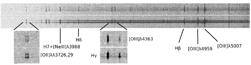
Figure 2: Reduced central block of fibres of quadrant Q2 for the observation of UM 461, OB HRB 3 (see Table 2). We labelled the most important emission lines.

The flux calibration was performed using the sensitivity function derived from observations of spectrophotometric standard stars included in the VIMOS-IFU calibration plan. The 2D data images were transformed into 3D data cubes, re-sampled to a 0.33$\arcsec$ spatial resolution. We correct for the quadrant-to-quadrant intensity differences following the procedure applied by Lagerholm et al. (2012) assuming that the intensity correction is uniform within each quadrant. Therefore, we renormalized the quadrants by comparing the intensity levels of the neighbouring pixels at the quadrant borders. When comparing the mean intensity value in quadrants Q1, Q3, and Q4 with respect to quadrant Q2 we found values of $\sim$0.2, $\sim$0.8 and $\sim$0.1, respectively. We checked the effects of the differential atmospheric refraction (DAR) in each data cube by calculating the centroid of the main emission regions in several monochromatic maps. We found in our worst case with an airmass of $\sim$1.5 (see Table 2) which had an offset of $\sim$2.2 spaxels near [O ii]$\lambda\lambda$3726,3729. While near [O iii]$\lambda$4363 (the critical emission line to determine O/H abundances) we found an offset of $\sim$1.41 spaxels. Therefore, we applied an IRAF-based script (Walsh & Roy, 1990) to correct for DAR. Finally, we note an offset in the pointing for some of those observations. The data cubes obtained using the HRB and HRO gratings were shifted and combined (using a sigma clipping algorithm to remove the cosmic rays) into a final data cube covering a useful spectral range from $\sim$3700 $\rm\AA$ to $\sim$7400 $\rm\AA$. This procedure also remove the dead fibres when averaging exposures. We scaled the HRB and HRO data cubes by comparing the integrated spectra of the galaxies with those obtained by Moustakas & Kennicutt (2006). This is a reasonable method given that there are no telluric lines in common in our HRB and HRO data cubes. Below, in this Section and Section 3 we find that the selected emission line ratios and other properties derived from the data cubes are in agreement, within the uncertainties, with those found in the literature. Finally, in Figure 3 we show the integrated spectra for each galaxy, obtained summing the spectra from all spaxels within the “Int” areas in Figure 1.

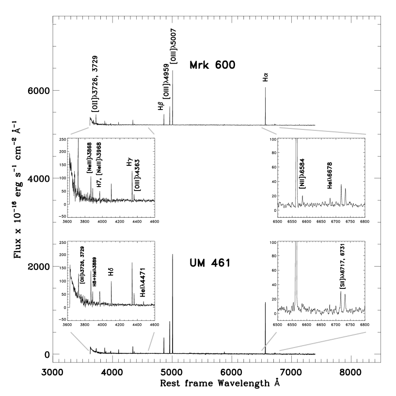
Figure 3: Integrated spectra for UM 461 and Mrk 600, with the inset panels showing wavelength ranges containing important named emission lines.

2.2 Emission line measurement

Line fluxes were measured, using IRAF tasks fitprofs and splot ([O ii]$\lambda\lambda$3726,3729), from a single Gaussian profile fit to each line. The spectral resolution of the VIMOS-IFU observations allowed us to resolve the [O ii]$\lambda\lambda$3726,3729 (see Figure 2) with a $\Delta\lambda$=2.95 $\rm\AA$ separation between the peaks of the lines in the integrated spectrum. The logarithmic reddening parameter c(H$\beta$) was calculated from the de-reddened raw flux data assuming case B (Osterbrock & Ferland, 2006) for the Balmer decrement ratio, H$\alpha$/H$\beta$=2.86 at 10,000 K. Then, the de-reddened emission line fluxes were calculated as

$$\frac{I(\lambda)}{I(H\beta)}=\frac{F(\lambda)}{F(H\beta)}\times 10^{c(H\beta)f(\lambda)}$$ (1)

where I($\lambda$) and F($\lambda$) are the de-reddened flux and observed flux at a given wavelength, respectively, and f($\lambda$) is the reddening function given by Cardelli, Clayton & Mathis (1989). In Table 3 we present for each galaxy the integrated observed F($\lambda$) and corrected emission-line fluxes I($\lambda$) relative to H$\beta$ (including uncertainties) multiplied by a factor of 100, the observed flux of the H$\beta$ emission line and the extinction coefficient c(H$\beta$). In Tables 4 and 5 we present the values for the resolved H ii regions (see Figure 1) within UM 461 and Mrk 600, respectively.

Table 3: UM 461 and Mrk 600: observed and de-reddened integrated emission line fluxes. The fluxes are relative to F(H$\beta$)=100.

	UM 461		Mrk 600
	F($\lambda$)/F(H$\beta$)	I($\lambda$)/I(H$\beta$)	F($\lambda$)/F(H$\beta$)	I($\lambda$)/I(H$\beta$)
$\left[OII\right]\lambda$3726	13.13$\pm$4.37	13.53$\pm$6.41	42.69$\pm$4.53	46.32$\pm$8.64
$\left[OII\right]\lambda$3729	26.53$\pm$4.49	27.33$\pm$6.47	86.15$\pm$9.15	93.46$\pm$17.44
$\left[NeIII\right]\lambda$3868	33.48$\pm$1.97	34.39$\pm$2.86	31.61$\pm$3.04	34.03$\pm$4.6
H8+He I $\lambda$3889	13.79$\pm$0.81	14.16$\pm$1.18	14.72$\pm$1.42	15.83$\pm$2.15
$\left[NeIII\right]\lambda$3968	11.71$\pm$0.70	11.00$\pm$1.74	14.08$\pm$0.23	15.06$\pm$0.35
H7 $\lambda$3970	10.93$\pm$0.64	11.20$\pm$0.93	14.85$\pm$1.43	15.88$\pm$2.16
H$\delta\lambda$4101	23.24$\pm$1.37	23.74$\pm$1.98	24.57$\pm$2.36	26.04$\pm$3.54
H$\gamma\lambda$4340	42.15$\pm$2.48	42.76$\pm$3.56	45.94$\pm$4.88	47.80$\pm$7.18
$\left[OIII\right]\lambda$4363	12.17$\pm$0.68	12.34$\pm$0.97	8.79$\pm$0.62	9.13$\pm$0.91
HeI $\lambda$4471	3.49$\pm$0.20	3.53$\pm$0.28	$\cdots$	$\cdots$
H$\beta\lambda$4861	100.00$\pm$1.78	100.00$\pm$2.52	100.00$\pm$1.24	100.00$\pm$1.75
$\left[OIII\right]\lambda$4959	204.16$\pm$4.05	203.68$\pm$5.71	168.80$\pm$6.41	167.71$\pm$9.00
$\left[OIII\right]\lambda$5007	643.80$\pm$7.76	641.56$\pm$10.94	496.16$\pm$6.68	491.44$\pm$9.36
H$\alpha\lambda$6563	294.97$\pm$3.62	286.99$\pm$4.98	311.56$\pm$7.12	288.94$\pm$9.34
$\left[NII\right]\lambda$6584	1.58$\pm$0.76	1.54$\pm$1.04	2.98$\pm$0.34	2.76$\pm$0.44
HeI $\lambda$6678	2.50$\pm$0.15	2.43$\pm$0.15	3.82$\pm$0.37	3.53$\pm$0.48
$\left[SII\right]\lambda$6717	8.18$\pm$0.28	7.94$\pm$0.38	11.24$\pm$0.49	10.37$\pm$0.64
$\left[SII\right]\lambda$6731	7.16$\pm$0.29	7.00$\pm$0.40	10.46$\pm$0.45	9.65$\pm$0.59
F(H$\beta$)	11.53$\pm$0.10		7.69$\pm$0.05
c(H$\beta$)	0.04$\pm$0.04		0.11 $\pm$0.07
log($\left[OIII\right]\lambda$5007/H$\beta$)	0.81$\pm$0.02		0.69$\pm$0.02
log($\left[NII\right]\lambda$6584/H$\alpha$)	-2.27$\pm$0.69		-2.02$\pm$0.19
log($\left[SII\right]\lambda\lambda$6717,6731/H$\alpha$)	-1.28$\pm$0.08		-1.16$\pm$0.09

Table 4: UM 461: observed and de-reddened emission line fluxes for regions no. 1 and no. 2. The fluxes are relative to F(H$\beta$)=100.

	Region no. 1		Region no. 2
	F($\lambda$)/F(H$\beta$)	I($\lambda$)/I(H$\beta$)	F($\lambda$)/F(H$\beta$)	I($\lambda$)/I(H$\beta$)
$\left[OII\right]\lambda$3726	8.42$\pm$0.93	$\ldots$	20.74$\pm$0.55	$\ldots$
$\left[OII\right]\lambda$3729	21.37$\pm$1.09	$\ldots$	38.31$\pm$5.10	$\ldots$
$\left[NeIII\right]\lambda$3868	32.72$\pm$1.75	$\ldots$	30.48$\pm$1.75	$\ldots$
H8+He I $\lambda$3889	12.34$\pm$0.66	$\ldots$	13.27$\pm$0.76	$\ldots$
$\left[NeIII\right]\lambda$3968	12.11$\pm$0.65	$\ldots$	9.71$\pm$0.56	$\ldots$
H7 $\lambda$3970	12.34$\pm$0.66	$\ldots$	13.77$\pm$0.79	$\ldots$
H$\delta\lambda$4101	23.87$\pm$1.28	$\ldots$	21.53$\pm$1.24	$\ldots$
H$\gamma\lambda$4340	43.66$\pm$2.34	$\ldots$	41.10$\pm$2.36	$\ldots$
$\left[OIII\right]\lambda$4363	13.94$\pm$0.39	$\ldots$	8.87$\pm$0.62	$\ldots$
HeI $\lambda$4471	3.35$\pm$0.18	$\ldots$	2.63$\pm$0.15	$\ldots$
H$\beta\lambda$4861	100.00$\pm$0.73	$\ldots$	100.00$\pm$1.48	$\ldots$
$\left[OIII\right]\lambda$4959	219.03$\pm$3.04	$\ldots$	186.82$\pm$4.37	$\ldots$
$\left[OIII\right]\lambda$5007	696.32$\pm$4.24	$\ldots$	564.41$\pm$6.40	$\ldots$
H$\alpha\lambda$6563	280.86$\pm$1.52	$\ldots$	253.88$\pm$2.91	$\ldots$
$\left[NII\right]\lambda$6584	1.16$\pm$0.60	$\ldots$	$\ldots$	$\ldots$
HeI $\lambda$6678	2.77$\pm$0.15	$\ldots$	$\ldots$	$\ldots$
$\left[SII\right]\lambda$6717	4.48$\pm$0.10	$\ldots$	6.24$\pm$0.24	$\ldots$
$\left[SII\right]\lambda$6731	3.63$\pm$0.18	$\ldots$	6.20$\pm$0.26	$\ldots$
F(H$\beta$)	$8.59\pm$0.03		1.02$\pm$0.01
c(H$\beta$)	0.00$\pm$0.02		0.00$\pm$0.03
log($\left[OIII\right]\lambda$5007/H$\beta$)	0.84$\pm$0.01		0.75$\pm$0.01
log($\left[NII\right]\lambda$6584/H$\alpha$)	-2.38$\pm$0.38		$\ldots$
log($\left[SII\right]\lambda\lambda$6717,6731/H$\alpha$)	-1.54$\pm$0.04		-1.31$\pm$0.06

Table 5: Mrk 600: observed and de-reddened emission line fluxes for regions no. 1, no. 2, no. 3 and no. 4. The fluxes are relative to F(H$\beta$)=100.

	Region no. 1		Region no. 2		Region no. 3		Region no. 4
	F($\lambda$)/F(H$\beta$)	I($\lambda$)/I(H$\beta$)	F($\lambda$)/F(H$\beta$)	I($\lambda$)/I(H$\beta$)	F($\lambda$)/F(H$\beta$)	I($\lambda$)/I(H$\beta$)	F($\lambda$)/F(H$\beta$)	I($\lambda$)/I(H$\beta$)
$\left[OII\right]\lambda$3726	18.05$\pm$1.90	20.48$\pm$3.05	41.41$\pm$4.35	47.33$\pm$7.03	51.60$\pm$5.41	$\ldots$	34.98$\pm$3.66	37.95$\pm$5.62
$\left[OII\right]\lambda$3729	33.93$\pm$3.57	38.48$\pm$5.73	70.90$\pm$7.44	81.01$\pm$12.02	104.44$\pm$10.96	$\ldots$	72.46$\pm$7.58	78.61$\pm$11.63
$\left[NeIII\right]\lambda$3868	40.43$\pm$3.85	45.31$\pm$6.10	22.43$\pm$2.13	25.31$\pm$3.40	29.04$\pm$2.76	$\ldots$	26.14$\pm$2.48	28.14 $\pm$3.77
H8+He I $\lambda$3889	14.78$\pm$1.41	16.53$\pm$2.23	12.27$\pm$1.16	13.82$\pm$1.85	17.42$\pm$1.65	$\ldots$	13.51$\pm$1.28	14.53 $\pm$1.95
$\left[NeIII\right]\lambda$3968	12.55$\pm$0.19	13.93$\pm$0.30	8.58$\pm$0.13	9.58$\pm$0.20	11.63$\pm$0.17	$\ldots$	11.35$\pm$0.17	12.14 $\pm$0.26
H7 $\lambda$3970	11.15$\pm$1.06	12.37$\pm$1.66	11.67$\pm$1.11	13.03$\pm$1.75	16.51$\pm$1.57	$\ldots$	12.83$\pm$1.21	13.72 $\pm$1.83
H$\delta\lambda$4101	23.98$\pm$2.28	26.24$\pm$3.53	19.84$\pm$1.88	21.82$\pm$2.92	25.83$\pm$2.45	$\ldots$	22.90$\pm$2.17	24.27 $\pm$3.25
H$\gamma\lambda$4340	46.47$\pm$4.89	49.41$\pm$7.35	4.06$\pm$0.43	4.33$\pm$0.65	47.68$\pm$5.00	$\ldots$	44.82$\pm$4.69	46.63 $\pm$6.90
$\left[OIII\right]\lambda$4363	12.00$\pm$0.53	12.72$\pm$0.79	6.58$\pm$0.45	7.00$\pm$0.68	7.21$\pm$0.46	$\ldots$	7.78$\pm$0.40	8.08 $\pm$0.59
HeI $\lambda$4471	3.46$\pm$0.33	3.62$\pm$0.49	3.28$\pm$0.31	3.44$\pm$0.46	3.19$\pm$0.30	$\ldots$	2.97$\pm$0.28	3.06 $\pm$0.41
H$\beta\lambda$4861	100.00$\pm$1.03	100.00$\pm$1.46	100.00$\pm$0.98	100.00$\pm$1.38	100.00$\pm$0.98	$\ldots$	100.00$\pm$0.94	100.00$\pm$1.33
$\left[OIII\right]\lambda$4959	213.15$\pm$6.00	211.02$\pm$8.40	144.81$\pm$4.86	143.28$\pm$6.80	146.61$\pm$4.78	$\ldots$	163.64$\pm$4.01	162.58$\pm$5.63
$\left[OIII\right]\lambda$5007	631.97$\pm$3.89	622.70$\pm$5.42	432.27$\pm$3.18	425.56$\pm$4.43	427.79$\pm$5.51	$\ldots$	489.78$\pm$4.89	485.12$\pm$6.85
H$\alpha\lambda$6563	325.87$\pm$7.88	290.04$\pm$9.92	328.54$\pm$7.12	292.42$\pm$9.34	241.73$\pm$5.85	$\ldots$	311.14$\pm$6.75	288.55$\pm$8.85
$\left[NII\right]\lambda$6584	1.59$\pm$0.24	1.41$\pm$0.30	3.17$\pm$0.27	2.80$\pm$0.34	2.61$\pm$0.26	$\ldots$	2.50$\pm$0.24	2.32$\pm$0.31
HeI $\lambda$6678	3.12$\pm$0.30	2.76$\pm$0.37	3.02$\pm$0.29	2.65$\pm$0.36	2.59$\pm$0.25	$\ldots$	3.63$\pm$0.34	3.35$\pm$0.44
$\left[SII\right]\lambda$6717	7.07$\pm$0.33	6.24$\pm$0.41	14.35$\pm$0.43	12.58$\pm$0.53	12.29$\pm$0.43	$\ldots$	11.80$\pm$0.36	10.89$\pm$0.47
$\left[SII\right]\lambda$6731	5.15$\pm$0.29	4.54$\pm$0.36	9.48$\pm$0.35	8.30$\pm$0.43	9.75$\pm$0.35	$\ldots$	9.65$\pm$0.32	8.90$\pm$0.42
F(H$\beta$)	2.12$\pm$0.01		0.57$\pm$0.01		0.64$\pm$0.01		2.00$\pm$0.01
c(H$\beta$)	0.17$\pm$0.07		0.18$\pm$0.06		0.00$\pm$0.07		0.11$\pm$0.06
log($\left[OIII\right]$)	0.79$\pm$0.01		0.63$\pm$0.01		0.63$\pm$0.01		0.68$\pm$0.01
log($\left[NII\right]$)	-2.31$\pm$0.25		-2.02$\pm$0.15		-1.97$\pm$0.12		-2.09$\pm$0.16
log($\left[SII\right]$)	-1.43$\pm$0.10		-1.15$\pm$0.08		-1.04$\pm$0.06		-1.16$\pm$0.08

3 Results

3.1 Emission lines, morphology and emission-line ratios

3.1.1 Emission lines and morphology

We used the flux measurements described in Section 2 to produce the following emission line maps: [S ii]$\lambda$6731, [S ii]$\lambda$6717, [N ii]$\lambda$6584, H$\alpha$, [O iii]$\lambda$5007, [O iii]$\lambda$4959, H$\beta$, [O iii]$\lambda$4363 and [O ii]$\lambda\lambda$3726,3729. In Figures 4 (UM 461) and 5 (Mrk 600) we show a selection of those maps. We note that, when deriving the maps we only use spaxels with emission fluxes $>$ 3$\sigma$ in the background observations. Our H$\alpha$ maps (Figure 1) reveal that the nebular emission is concentrated in the main bodies of both UM 461 and Mrk 600 and the centres are coincident with the continuum emission maxima (see Lagos et al., 2007). However, extended diffuse ionized gas emission surrounding the GH iiRs is also observed within the VIMOS-IFU FoVs for both galaxies. In UM 461, we resolve two regions or GH iiRs labelled as regions no. 1 and no. 2 in Figure 1 (upper right panel) as well as several adjacent faint structures. We compared the UM 461 [O ii], [O iii], [S ii], [N ii] forbidden emission line morphologies to that of the H$\alpha$ emission. The morphologies for emission lines closely match each another, although due to our sensitivity limit the extent of the H$\alpha$ and [O iii]$\lambda$5007 emission is larger than those of [O ii]$\lambda\lambda$3726,3729, [S ii]$\lambda\lambda$6717,6731, [O iii]$\lambda$4363 and [N ii]$\lambda$6584 (see Figure 4).

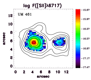
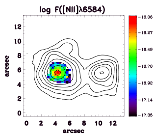
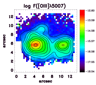
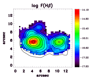
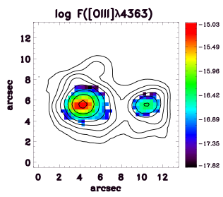
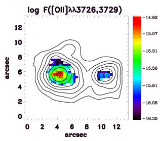
Figure 4: UM 461 - Emission line maps: [S II]$\lambda$6717, [N II]$\lambda$6584, [O III]$\lambda$5007, H$\beta$, [O III]$\lambda$4363 and [O II]$\lambda\lambda$3726,3729. H$\alpha$ emission line contours are overlaid on each map. North is up and east is to the left.

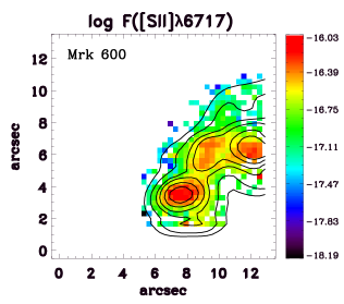
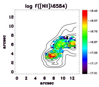
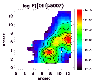
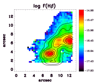
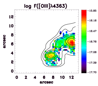
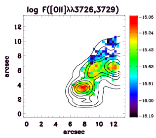
Figure 5: Mrk 600 - Emission line maps: [S II]$\lambda$6717, [N II]$\lambda$6584, [O III]$\lambda$5007, H$\beta$, [O III]$\lambda$4363 and [O II]$\lambda\lambda$3726,3729. H$\alpha$ emission line contours are overlaid on each map. North is up and east is to the left.

Overall, the H$\alpha$ emission of Mrk 600 displays an elongated morphology and four GH iiRs are labelled regions no. 1 to 4 on the H${\alpha}$ map (Figure 1 lower right panel). As for UM 461, the spatial distribution of recombination lines (H$\alpha$, H$\beta$, etc.) in Mrk 600 is very similar to the emission from forbidden lines (see Figure 5). Interestingly, we observe two extended structures or shells, adjacent to region no. 1 (see Figure 1 lower right). H$\alpha$ narrow-band images presented by Gil de Paz, Madore & Pevunova (2003) and Janowiecki & Salzer (2014) show that both structures are very well resolved. This confirms the presence of an extended shell, or bubble, that is $\sim$180 pc away from the H$\alpha$ peak of region no. 1.

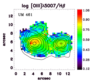
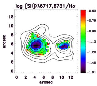
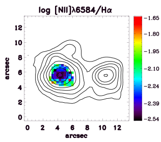
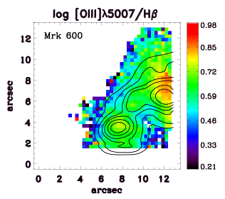
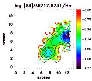
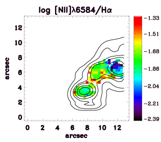
Figure 6: Emission line ratio maps: log [O III]$\lambda$5007/H$\beta$, log [S II]$\lambda\lambda$6717,6731/H$\alpha$ and log [N II]$\lambda$6584/H$\alpha$ for UM 461 (upper panels) and Mrk 600 (lower panels). H$\alpha$ emission line contours are overlaid on each map. North is up and east is to the left.

3.1.2 Emission-line ratios

For both UM 461 and Mrk 600, we employed the commonly used BPT (Baldwin, Phillips & Terlevich, 1981) diagrams to infer the dominant ionization mechanism at spaxel scales using the following emission-line ratios: [O iii]$\lambda$5007/H$\beta$, [S ii]$\lambda\lambda$6717,6731/H$\alpha$ and [N ii]$\lambda$6584/H$\alpha$ (see Figure 6). The spatial profiles of the emission line ratios differ significantly from one another, as shown in Figure 6, between the peak of the H$\alpha$ emission and the edge of the VIMOS-IFU FoV. The ionization structure within the inner most part of the GH iiRs, for both galaxies, is rather constant as measured by [S ii]$\lambda\lambda$6717,6731/H$\alpha$ and [N ii]$\lambda$6584/H$\alpha$, but these ratios increase at greater distances from the GH iiRs. However, the [O iii]$\lambda$5007/H$\beta$ ratios do not show a uniform distribution. In the case of UM 461 its values are highest in a curved structure, which surrounds the peak of H$\alpha$ emission. Our [O iii]$\lambda$5007/H$\beta$ ratio map, in this galaxy, is in excellent agreement with the map obtained by Sampaio Carvalho (2013) using Gemini Multi-Object Spectrograph (GMOS) IFU. We do not show, in this paper, the BPT diagrams but all points fall in the locus predicted by models of photo-ionization by young stars in H ii regions (Osterbrock & Ferland, 2006), indicating that photoionization from stellar sources is the dominant excitation mechanism in UM 461 and Mrk 600. We compared the aforementioned integrated emission line ratios, for both galaxies, showed in Table 3 with the values found in the literature. Our values obtained in UM 461 are in agreement, within the uncertainties, with those reported by Pérez-Montero & Díaz (2003), i.e., log([O iii]$\lambda$5007/H$\beta$) = 0.78, log([S ii]$\lambda\lambda$6717,6731/H$\alpha$) = -1.47 and log([N ii]$\lambda$6584/H$\alpha$) = -2.12. Finally, the emission line ratios in Mrk 600 (see Tables 3 and 5) are in agreement with those from Guseva et al. (2011), i.e., log([O iii]$\lambda$5007/H$\beta$) = 0.81, log([S ii]$\lambda\lambda$6717,6731/H$\alpha$) = -1.46 and log([N ii]$\lambda$6584/H$\alpha$) = -2.07.

3.2 Abundance determinations

For our abundance estimates, we first determined the electron temperature T_e and electron density n_e, making use of the line ratios [O iii]$\lambda$4959,5007/[O iii]$\lambda$4363 and [S ii]$\lambda$6716/[S ii]$\lambda$6731, and the IRAF STS package nebular.

Oxygen and nitrogen ion abundances O⁺, O⁺⁺ and N⁺ were calculated using the five-level atomic model FIVEL implemented in the IRAF STS task abund. The total oxygen abundance for each aperture is obtained assuming the contributions from O⁺ and O⁺⁺, therefore we have:

$$\frac{O}{H}=\frac{O^{+}}{H^{+}}+\frac{O^{++}}{H^{+}},$$ (2)

and

$$\frac{N}{H}=ICF(N)\frac{N^{+}}{H^{+}},$$ (3)

with

$$ICF(N)=\frac{O^{+}+O^{2+}}{O^{+}}.$$ (4)

In Figure 7, we show the oxygen abundance and the log(N/O) ratio maps in the left and right panels, for both UM 461 and Mrk 600. Tables 6 and 7, respectively, show the abundances measured for the individual apertures within the FoVs of UM 461 and Mrk 600 (see Figure 1). Our integrated oxygen abundances of 12 + log(O/H) = 7.84$\pm$0.08 and 7.85$\pm$0.09 are in agreement with those in Izotov & Thuan (1998) of 7.78$\pm$0.03 and 7.83$\pm$0.01 for UM 461 and Mrk 600, respectively. For UM 461 a larger discrepancy however occurs with the value of 7.32$\pm$0.15 from Sánchez Almeida et al. (2015). In the case of Mrk 600, the difference between the oxygen abundances of the GH iiRs 2, 3 and 4 and region no. 1 is $\Delta$(O/H) $\leq$ 0.04 dex, while in UM 461 we find a difference of $\Delta$(O/H) = 0.06 dex between the two main regions. Therefore, within the uncertainties we can consider that the oxygen abundances amongst and between the GH iiRs of each galaxy are similar. The 12 + log(O/H) values in Figure 7 range from 7.38 to 8.30 for UM 461 and from 7.40 to 8.35 in Mrk 600. In Mrk 600 the lowest values of 12 + log(O/H) ($<$ 7.6) are found surrounding the brightest regions (no. 1 and no. 4). For UM 461 the lowest values of 12 + log(O/H) are in the southern part of region no. 1 with an extent of $\sim$0.7 kpc oriented towards the faint SW stellar tail (see Figure 1 upper right). This region has a mean 12 + log(O/H) value of $\sim$7.52 and a difference of $\Delta$(O/H) = 0.46 dex between the lowest abundance and the integrated value. Interestingly, this region is not coincident with the peak of H$\alpha$ emission or other star clusters resolved by Lagos et al. (2011) within our region no. 1.

In order to test the accuracy in the detection of variations of oxygen abundance, we introduced several offsets of 0.33$\arcsec$ (one spaxel) in the [O iii]$\lambda$4363 maps. In most cases (75%), we found that the spatial variations are preserved within 0.1 dex. Given that the seeing during our observations was $\sim$1.0$\arcsec$ (3 spaxels), the pixel-to-pixel variation in our maps are potentially due to measurement uncertainties rather than real variations. This point is commonly ignored in most of the IFU studies. To further test whether the variations were real or not, we binned the data cube from 0.33$\arcsec$ to $\sim$1.0$\arcsec$ (3 spaxels). In Figure 8 we show the spatial distribution of the binned ($\sim$1$\arcsec$ spaxel) 12 + log(O/H) abundances. Again, in both cases the abundance patterns are preserved. Nevertheless, it is more practical for the analysis to use the 0.33$\arcsec$ pixel scale.

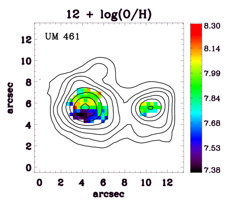
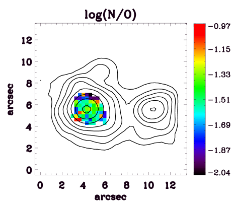
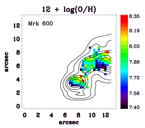
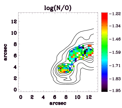
Figure 7: 12 + log(O/H) and log(N/O) abundance maps for UM 461 (upper panels) and Mrk 600 (lower panels). Oxygen abundances were determined using using the direct method. H$\alpha$ emission line contours are overlaid on each map. North is up and east is to the left.

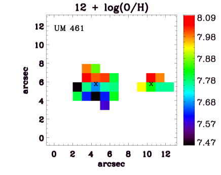
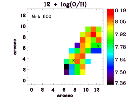
Figure 8: Spatial distribution of the binned ($\sim$1$\arcsec$ spaxels) 12 + log(O/H) abundances for both galaxies UM 461 (upper panel) and Mrk 600 (lower panel). The maximum H$\alpha$ emission of the main regions are indicated in the maps by a X symbol. North is up and east is to the left.

We find an integrated value of 12 + log(N/H) = 6.31$\pm$0.18 for UM 461 and 6.03$\pm$0.22 for Mrk 600. The nitrogen-to-oxygen ratio in these galaxies is log(N/O) = -1.54$\pm$0.27 and -1.83$\pm$0.30 for UM 461 and Mrk 600, respectively. In the case of UM 461, the integrated log(N/O) is consistent with those found in XMP galaxies (log(N/O) $\sim$ -1.60; e.g. Edmunds & Pagel, 1978; Alloin et al., 1979; Izotov & Thuan, 1999). Interestingly, the region no. 1 in UM 461 and the area of low metallicity, in the same region, show a similar log(N/O) value $\sim$ -1.50. Therefore, the log(N/O) ratio is uniform at large scales in the brightest region of this galaxy. Finally, we found that the integrated log(N/O) values agree, within the uncertainties, with those obtained by Izotov & Thuan (1998), i.e., log(N/O) = -1.50 for UM 461 and of -1.67 for Mrk 600.

Table 6: UM 461: ionic abundances and integrated properties.

	Integrated	Region no.1	Region no.2
Te(OIII) K	15184$\pm$548	15487$\pm$288	13838$\pm$576
Ne(SII) cm-3	431$\pm$223	208$\pm$172	662$\pm$286
O+/H${}^{+}\times$105	0.50$\pm$0.03	0.34$\pm$0.01	0.87$\pm$0.06
O++/H${}^{+}\times$105	6.49$\pm$0.59	6.71$\pm$0.31	7.32$\pm$0.83
O/H $\times$105	6.99$\pm$0.62	7.04$\pm$0.32	8.19$\pm$0.88
12 + log(O/H)	7.84$\pm$0.08	7.85$\pm$0.05	7.91$\pm$0.10
N+/H${}^{+}\times$106	0.14$\pm$0.01	0.11$\pm$0.01	$\ldots$
ICF(N)	14.08$\pm$2.11	21.74$\pm$1.52	9.46$\pm$1.65
N/H $\times$106	2.02$\pm$0.36	2.24$\pm$0.20	$\ldots$
12+log(N/H)	6.31$\pm$0.18	6.35$\pm$0.09	$\ldots$
log(N/O)	-1.54$\pm$0.27	-1.50$\pm$0.14	$\ldots$

Table 7: Mrk 600: ionic abundances and integrated properties.

	Integrated	Region no.1	Region no.2	Region no.3	Region no.4
Te(OIII) K	14825$\pm$670	15491$\pm$462	14075$\pm$580	14200$\pm$558	14156$\pm$438
Ne(SII) cm-3	502$\pm$134	30$\pm$110	$\sim$100	170$\pm$110	222$\pm$93
O+/H${}^{+}\times$105	1.78$\pm$0.12	0.63$\pm$0.03	1.63$\pm$0.11	1.99$\pm$0.13	1.51$\pm$0.07
O++/H${}^{+}\times$105	5.37$\pm$0.62	6.12$\pm$0.45	5.33$\pm$0.59	5.25$\pm$0.55	5.97$\pm$0.49
O/H $\times$105	7.16$\pm$0.75	6.76$\pm$0.48	6.96$\pm$0.70	7.24$\pm$0.67	7.48$\pm$0.56
12 + log(O/H)	7.85$\pm$0.09	7.83$\pm$0.07	7.84$\pm$0.09	7.86$\pm$0.09	7.87$\pm$0.09
N+/H${}^{+}\times$106	0.26$\pm$0.01	0.13$\pm$0.01	0.28$\pm$0.01	0.26$\pm$0.01	0.23$\pm$0.01
ICF(N)	4.01$\pm$0.69	10.66$\pm$1.24	4.27$\pm$0.71	3.64$\pm$0.57	4.95$\pm$0.62
N/H $\times$106	1.06$\pm$0.24	1.39$\pm$0.20	1.21$\pm$0.26	0.95$\pm$0.19	1.15$\pm$0.18
12+log(N/H)	6.03$\pm$0.22	6.14$\pm$0.15	6.08$\pm$0.22	5.98$\pm$0.20	6.06$\pm$0.16
log(N/O)	-1.83$\pm$0.30	-1.69$\pm$0.22	-1.76$\pm$0.30	-1.88$\pm$0.29	-1.81$\pm$0.24

3.3 Velocity fields

We obtained the radial velocity v_r(H$\alpha$) by fitting a single Gaussian to the H$\alpha$ emission line profiles. The v_r(H$\alpha$) velocity fields showed in Figure 9 are rather complex. For UM 461 the velocity field shows an apparently systemic trend with the northern part redshifted, while the southern part is blueshifted, with a systemic velocity of $\sim$1040 km s^-1. As mentioned in Section 1, this galaxy is part of a binary system with UM 462. Interestingly, the velocity distribution in UM 462 shows no spatial correlation with the H$\alpha$ emission (see Figure 2 in James, Tsamis & Barlow, 2010). A similar lack of correlation is observed in UM 461. The range of radial velocities displayed in the UM 461 map is about 60 km s^-1, while the velocity difference between regions no. 1 and no. 2 is $\sim$ 13 km s^-1. The UM 461 V_r(H$\alpha$) velocity field shows the same overall pattern and detailed variations as the velocity field reported by Sampaio Carvalho (2013) from GMOS-IFU observations. Our IFU observations did not detect asymmetric line profiles or multiple components in the base of H$\alpha$ profile as observed by Olmo-García et al. (2017) from their 1$\arcsec$-width long-slit observation.

In the case of Mrk 600, despite of the small VIMOS FoV, we observe that the southwestern part of the galaxy is slightly blueshifted with respect to the systemic velocity of 1016 km s^-1. The variation in velocity within the Mrk 600 VIMOS-IFU FoV is $\sim$30 km s^-1. The v_r(H$\alpha$) maximum, in Mrk 600, is located very closed to region no. 2, the position where an expanding shell has been reported, while the minimum is near to region no. 1.

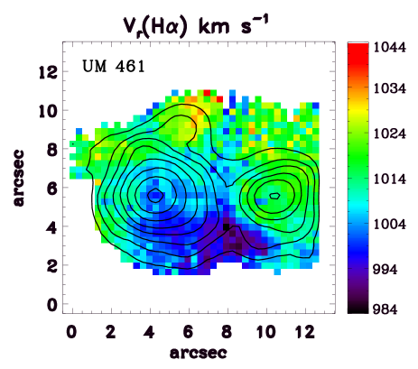
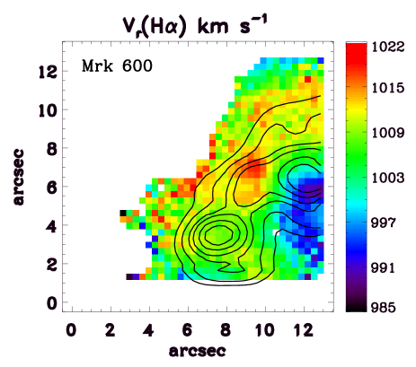
Figure 9: Radial velocity of the H$\alpha$ emission line in units of km s^-1 for UM 461 and Mrk 600. Contours display the H$\alpha$ morphology of the galaxies. North is up and east is to the left.

4 Discussion

4.1 Spatial variation of oxygen abundance

Here, we characterize the spatial distribution and variation of oxygen abundance found in Section 3.2. In Figure 10 we show histograms of the distribution of the 12 + log(O/H) spaxel values for UM 461 (upper panel) and Mrk 600 (lower panel). The dotted lines in the Figure indicate the mean 12 + log(O/H) values of 7.81 and 7.84; with the same standard deviations of $\sim$0.21 for UM 461 and Mrk 600, respectively. We note that the mean value of these distributions agree at the 1$\sigma$ level with the integrated 12 + log(O/H) values for the galaxies in Tables 6 and 7. Interestingly, in the case of Mrk 600 the distribution can be fitted by a single Gaussian, while in the case of UM 461 the distribution is well fitted by two Gaussian components.

Following the statistical analysis in Pérez-Montero et al. (2011) and Kehrig et al. (2016) we consider the two conditions for oxygen abundance to be considered homogeneous: i) the derived values of 12 + log(O/H) should be fitted by a normal distribution according to the Lilliefors test and ii) the observed variations of the data distribution around the mean values $\sigma_{Gaussian}$ should be lower or of the order of the typical uncertainty of the property considered. The dispersion of the normal distribution $\sigma_{Gaussian}$ in Mrk 600 is of the order of the uncertainty of the oxygen abundance, estimated as the square root of the weighted variance of the data points $\sigma_{weighted}\sim 0.21$ . While, in UM 461 $\sigma_{Gaussian}$ (=0.20) $>\sigma_{weighted}$ (=0.17). Individual statistical analysis of the Gaussian components in UM 461 shows that $\sigma_{Gaussian}\lesssim\sigma_{weighted}$. Those results indicate that at large scales the ISM is chemically homogeneous. In addition, we checked the null hypothesis that the data come from a normally distributed population by applying the Lilliefors test. From this, we do not have enough evidence to conclude that the data in Mrk 600 were not drawn from a normal distribution (p-value $\sim$0.5). However, we find that the p-value of the Lilliefors test for UM 461 is $\sim$0.0001, then it is significantly non-normal. Finally, given that for each galaxy the mean of the 12 + log(O/H) spaxel value distribution agrees with the integrated value, the spatial variations observed in UM 461 cannot be understood as only statistical fluctuations (Pérez-Montero et al., 2011).

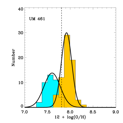
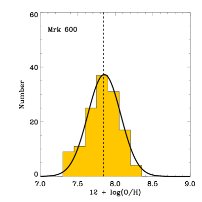
Figure 10: Histograms showing the distribution of 12 + log(O/H) spaxel values for UM 461 (upper panel) and Mrk 600 (lower panel). For each galaxy, the mean of the 12 + log(O/H) spaxel values (7.81 and 7.84, respectively) is indicated with a dotted line. The Figure also shows Gaussian fits to the distributions.

We conclude that the spatial variation and extended low metallicity region in UM 461 appear to be real, within our uncertainties, and it could indicate the recent infall of non-pristine metal-poor gas into the galaxy. Alternatively, it could be produced by the outflow of a large amount of enriched gas, consequently diminishing the metal content in this region. Below in this Section we discuss those scenarios in the context of the main properties of the ISM and the triggering of star-formation.

4.2 Oxygen abundance derivation using different diagnostics

In this Section we compute oxygen abundances using several different diagnostics and calibrations. First, the 12 + log(O/H) abundance was derived by applying the relation between the line ratio of [N ii]$\lambda$6584/H$\alpha$ with the oxygen abundance (N2; Denicoló, Terlevich, & Terlevich, 2002), i.e., 12 + log(O/H) = 9.12 + 0.73 $\times$ N2, with N2 = log ([N ii] $\lambda$6584/H$\alpha$). One of the most common methods used for estimating the oxygen abundance of metal-rich galaxies (12 + log(O/H) $\gtrsim$ 8.4) and also metal-poor galaxies (12 + log(O/H) $\lesssim$ 8.4) utilizes the R23 = (([O ii]$\lambda$3727 + [O iii]$\lambda\lambda$4959,5007)/H$\beta$) parameter, which is the ratio of the flux in the strong optical oxygen lines relative to H$\beta$. Applying this method the oxygen abundance, in our case, is given by the metal-poor branch 12 + log(O/H) = 7.056 + 0.767 x + 0.602 x² - y(0.29 + 0.332 x - 0.331 x²), where x = log(R23) and y = log(O32) = log([O iii]$\lambda\lambda$4959,5007)/[O ii]$\lambda\lambda$3726,3729) (R23; Kobulnicky et al., 1999). Another widely used indicator of oxygen abundance is given by 12 + log(O/H) = 8.73 - 0.32 $\times$ O3N2, where O3N2 = log([O iii] $\lambda$5007/H$\beta$ $\times$ H$\alpha$/[N ii] $\lambda$6584) (O3N2; Pettini & Pagel, 2004). Additionally, we use a new calibrator which has a weak dependence on the ionization parameter given by 12 + log(O/H) = 8.77 + Y, where Y = log([N ii] $\lambda$6584/[S ii]$\lambda\lambda$6717,6731) + 0.264 $\times$ N2 (D2016; Dopita et al., 2016). In order to cross check our results with previous determinations in the literature (e.g. Sánchez Almeida et al., 2015) we use the code HII–CHI–mistry version 2.1 (Pérez-Montero, 2014) which is a python program that calculates the 12 + log(O/H) abundance for gaseous nebulae ionized by massive stars using a set of emission-line optical intensities, i.e., [O ii]$\lambda$3727/H$\beta$, [O iii]$\lambda$4363/H$\beta$, [O iii]$\lambda$5007/H$\beta$, [N ii]$\lambda$6584/H$\beta$ and [S ii]$\lambda\lambda$6717,6731/H$\beta$.

For UM 461 we simulated long-slit observations along the main body of the galaxy, assuming a slit width of $\sim$1$\arcsec$. Figure 11 shows the radial profile of the oxygen abundance with respect to the UM 461 peak of H$\alpha$ emission using the direct method (determination of oxygen abundance using the T_e) compared to oxygen abundances determined using the other methods described above.

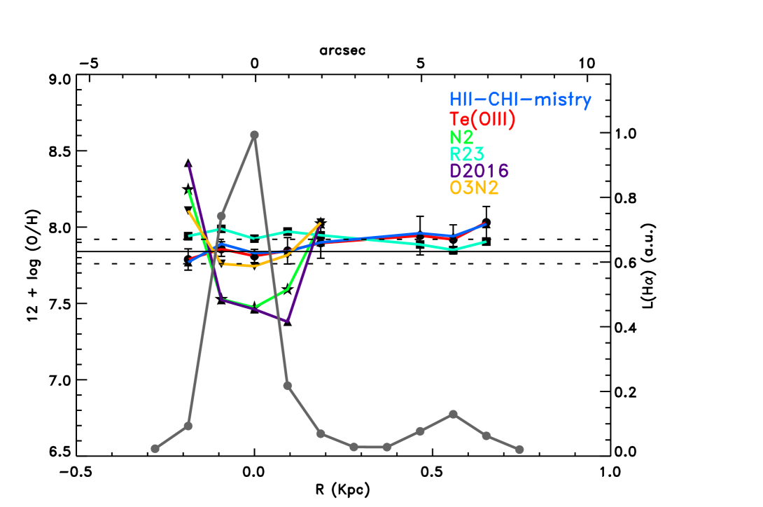
Figure 11: UM 461: radial distribution of oxygen abundance for simulated long slit observations across the main body of the galaxy. Six determinations of oxygen abundance are indicated in this Figure: i) the direct method (circles, red line), ii) N2 (stars, green line), iii) R23 (squares, cyan line), iv) O3N2 (upside down triangle, orange line), v) D2016 (triangles, purple line) calibrators and vi) HII–CHI–mistry (triangles, blue line). The integrated 12 + log(O/H) = 7.84$\pm$0.08 obtained for UM 461 is represented by the horizontal black line, with its 1$\sigma$ error indicated with dotted lines. We also include the normalized H$\alpha$ luminosity (L) profile (gray line and dots), with the maxima at regions no. 1 and no. 2.

The integrated oxygen abundance in region no. 2 of UM 461, based on T_e(O iii), was determined to be 0.06 dex higher than in region no. 1. This difference is reflected in the slight gradient observed in Figure 11. In this Figure we see that the R23 method provides similar values for 12 + log(O/H) as the direct method within the uncertainties. On the other hand, the values based on the empirical N2 calibration in region no. 1 are $\sim$0.4 dex lower than those obtained from the direct method. Using D2016 gives the same relative values compared to N2. The oxygen abundances obtained using the O3N2 calibrator provide a similar lower but less extreme profile compared to those obtained using the N2 and D2016 calibrations. However, most of its values agree within the uncertainties with the ones found by the direct method. We find a good agreement between abundances computed using HII–CHI–mistry and by the direct method. It is clear that using the N2 and D2016 methods alone to study the spatial variation of oxygen abundance underestimates the abundance profile in region no. 1.

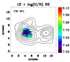
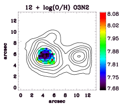
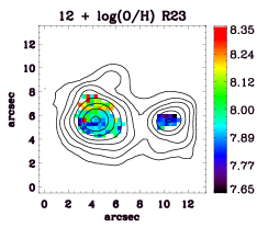
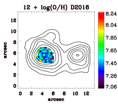
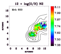
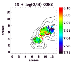
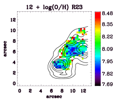
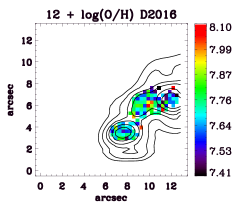
Figure 12: 12 + log(O/H) maps for UM 461 (Top row) and Mrk 600 (Bottom row) obtained using the N2, O3N2, R23 and D2016 calibrators. Contours display the H$\alpha$ morphology of the galaxies. North is up and east is to the left.

In Figure 12 we show the 12 + log(O/H) maps, for both galaxies, obtained using the N2, O3N2, R23 and D2016 oxygen abundance calibrators. From this Figure we observe significant spatial differences between the absolute values in the direct method maps compared to maps derived using some of the calibrators. The N2 and O3N2 abundance maps show spatial trends that are opposite to those shown by the other methods. Interestingly, both N2 and O3N2 show the lowest values in the regions of higher star-formation. Despite the fact that a detailed analysis is beyond the scope of the present paper, these results suggest a dependence on the ionization parameter $U$ (e.g. Kewley & Dopita, 2002). This value can be measured from the ratio of high ionisation to low ionisation species [O iii]$\lambda$5007/[O ii]$\lambda\lambda$3726,3729 using the parametrisation presented by Díaz et al. (2000), i.e., log($U$) = -0.8$\times$log([OII]/[OIII]) - 3.02 and also by the emission line ratio [S ii]$\lambda\lambda$6717,6731/H$\alpha$, log($U$) = -1.66$\times$log([SII]/H$\alpha$) - 4.13 (Dors et al., 2011). In Figure 13 we show the log($U$) maps for both galaxies. Clearly, the log($U$) is highest at the position of the GH iiRs and decreases radially outwards. The spatially resolved shape of abundances based on N2 and O3N2 correlates with the ionisation parameter. The shape and relative values of R23 maps agrees reasonably well with the direct method indicating only a weak dependence on $U$ in our sample of H ii/BCDs (e.g. Kehrig et al., 2016, and references therein). While, the D2016 maps does not closely correlate with the direct method and the log($U$) maps. The latter assumes the ISM conditions in high-z galaxies, which differ from those found in local galaxies. In Table 8 we show the mean values of 12 + log (O/H) obtained from the different methods. We find a difference between the mean value of R23 and the direct method of 0.16 dex and 0.23 dex for UM 461 and Mrk 600, respectively. While, the N2 and D2016 methods underestimate the mean oxygen abundance in UM 461. In summary, we conclude that most of the above methods provide a reasonable estimation of the integrated oxygen abundance, but some are less suited for a detailed study of spatial variations within the ISM of our BCDs. The observed variation of line ratios could be due to variations of $U$ instead of real metallicity variations. Below, we consider HII–CHI–mistry as a reliable tracer of the spatially resolved oxygen abundance when compared to the direct method.

Table 8: Statistical properties of 12 + log (O/H) using different methods.

	UM 461		Mrk 600
	Mean	STD	Mean	STD
Te	7.81	0.21	7.84	0.21
N2	7.59	0.16	7.85	0.17
O3N2	7.81	0.10	7.96	0.10
R23	7.97	0.14	8.07	0.14
D2016	7.51	0.20	7.75	0.16
HCM with [O iii]$\lambda$4363	7.83	0.21	7.86	0.21
HCM without [O iii]$\lambda$4363	7.94	0.15	8.02	0.13

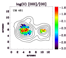
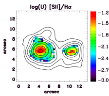
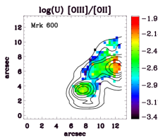
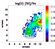
Figure 13: Ionisation parameter $U$ as mapped from Díaz et al. (2000) ([O iii]/[O ii]) and Dors et al. (2011) ([S ii]/H$\alpha$), for UM 461 (upper panels) and Mrk 600 (lower panels). Contours display the H$\alpha$ morphology of the galaxies.

We create the oxygen abundance maps (see Figure 14, inset panels) of the galaxies using the HII–CHI–mistry code as indicated above. It is important to note that the results obtained by using HII–CHI–mistry provide abundances that are consistent with the direct method, only when the [O iii]$\lambda$4363/H$\beta$ intensity is included. In order to better illustrate this, in Figure 14 we show the spaxel by spaxel comparison between 12 + log(O/H) derived using the direct method and HII–CHI–mistry (Pérez-Montero, 2014) with (left panels) and without (right panels) [O iii]$\lambda$4363 emission for UM 461 (upper panels) and Mrk 600 (lower panels), respectively. From this, we find a mean difference between the direct method and HII-CHI-mistry of $\mid\Delta$(O/H)$\mid=$0.02 dex for both galaxies (see Table 8) when we include the [O iii]$\lambda$4363 intensity. While the mean difference without [O iii]$\lambda$4363 is 0.13 dex and 0.18 dex for UM 461 and Mrk 600, respectively. These checks show consistency with the values obtained in Section 3.2 and also in Figure 11, when [O iii]$\lambda$4363 emission is included as an input for the code. We note that when we use [O iii]$\lambda$4363/H$\beta$ the code overestimate the abundances (Sánchez Almeida et al., 2016) as compared to the direct method at 12 + log (O/H) $\lesssim$ 7.6. These differences are small compared with their uncertainties. However, the 12 + log(O/H) abundance maps created with and without [O iii]$\lambda$4363 emission do not show any spatially consistency each other.

In the case of UM 461 our results (see Figure 11) differ from those in Olmo-García et al. (2017), whose values appear consistent with using HII–CHI–mistry, excluding the [O iii]$\lambda$4363 intensity. We therefore conclude that using HII–CHI–mistry recovers the oxygen abundance values, within the errors, and spatial variation of abundances obtained with the use of the direct method, only when the [O iii]$\lambda$4363/H$\beta$ intensity is included. We emphasise that our results clearly show that metallicity can appear to drop in regions of high star-formation activity (see Figure 14) if [O iii]$\lambda$4363 emission is not considered, which can lead to a misinterpretation of the real variation of oxygen abundances across the objects. Therefore, special attention must be paid to which emission lines are used when the HII–CHI–mistry method is applied to the study of spatial variation of abundances.

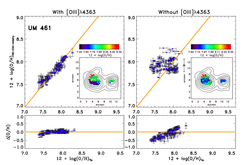
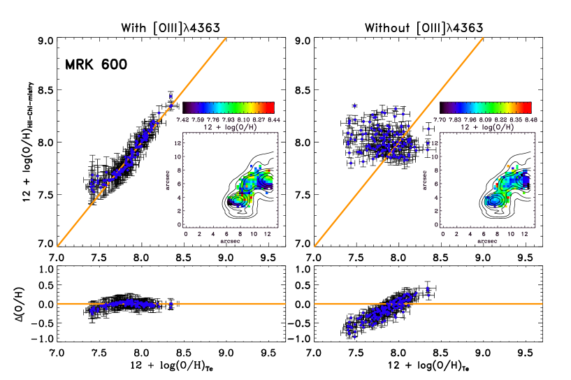
Figure 14: Spaxel by spaxel comparison between 12 + log(O/H) derived using HII-CHI-mistry (Pérez-Montero, 2014) and the T_e method for the galaxies UM 461 (upper panels) and Mrk 600 (lower panels). $\Delta$(O/H) is defined as log(O/H)${}_{T_{e}}$ - log(O/H)_{HII-CHI-mistry}. Contours display the H$\alpha$ morphology of the galaxies.

4.3 Spatially resolved star-formation, starburst properties and chemical abundances

In this Section, we discuss whether or not the observed star-formation traced by H${\alpha}$ correlates with the estimated oxygen abundance at spaxel scales. The current star-formation rate (SFR) was inferred from the extinction-corrected H$\alpha$ emission and the Kennicutt (1998) formula, after correction for a Kroupa initial mass function (Calzetti et al., 2007). Accordingly, we found a SFR = 0.077 M_⊙ yr^-1 and $>$0.017 M_⊙ yr^-1 for UM 461 and Mrk600, respectively. In the case of Mrk 600, an important fraction of the ISM is outsize the FoV (see Figure 1), then we found a lower limit for the SFR in this object. Note that, following common practice, SFRs are estimated from the H$\alpha$ luminosity and assuming solar metallicity. We caution that this standard conversion relies on two certainly overly simplistic assumptions commonly made, namely that a) star-forming activity is occurring continuously at a constant SFR for at least 100 Myr and b) Lyman photon escape is negligible. Using the 12 + log(O/H) from Section 3.2, in Figure 15 we show the spatially resolved relation between the Log($\Sigma_{SFR}$) and the oxygen abundance in UM 461 and Mrk 600.

UM 461. No correlation is found between the SFR and 12 + log(O/H) at spaxel scales in this galaxy. However, the spatial distribution of its oxygen abundance shows an extended area with a low value (12 + log(O/H) $<$ 7.6) in the southern part of region no. 1, as noted in Section 3.2. The metallicity in this region appears to decrease with increasing distance from cluster no. 2 and it increases when approaching cluster no. 3 (Figure 1 top right). Therefore, the lowest abundance of this off-centre region does not correlate with any of the aforementioned star clusters. The same behaviour is observed in the cometary galaxy Tol 65 (Lagos et al., 2016).

If we assume that UM 461 has recently experienced a single intense starburst, or series of starbursts, then the relatively oxygen deficient region could be the result of intensive starburst, then ejecting part of the pre-enriched gas (Veilleux, Cecil & Bland-Hawthorn, 2005, and references therein). Since different elements are produced on different time scales, it is expected that such a sequence of bursts would decrease the N/O ratio when massive stars die. However, the N/O is quite homogeneous indicating that the outflowing material is uniform and well mixed. In that case the N/O ratio is unchanging (van Zee & Haynes, 2006) within the uncertainties. This interpretation is consistent with the N/O ratio map in Figure 7. The age of the aforementioned clusters are $\sim$1 Myr and $\sim$4 Myr for clusters no. 2 and 3 respectively (Lagos et al., 2011). If we assume that the velocity, $v_{exp}=D/t_{exp}$, of the expanding material is constant, we obtain an outflow velocity of $\sim$340 km s^-1 after 1 Myr of expansion. This assumes that the radius D of the low metallicity region is an approximation of the distance from the star cluster no. 2 to the shock front. This scenario is plausible and indicates that supernovae (SNe) and stellar outflows, in UM 461, are capable of depleting the surrounding gas during the current starburst. In this circumstance metals ejected out of the ISM by supernovae-driven outflows are not completely lost (Silich & Tenorio-Tagle, 2001) into the intergalactic medium. The presence of broad components in the line profiles of the strongest emission lines would provide evidence of such fast motions (e.g. Bordalo & Telles, 2011), but these profiles are not detected in UM 461.

On the other hand interpreting the UM 461 metal-poor region as the consequence of a recent infall of metal-poor gas (e.g. Köppen & Hensler, 2005) implies the scatter in Figure 15 (left panel) arises because the metal-poor gas is not fully dispersed and mixed into the ISM. In this view, the star-formation activity in UM 461 started recently, in agreement with the findings by Lagos et al. (2011). Infalling gas from the outskirts of the galaxy could have triggered this star-formation activity (e.g. Ekta & Chengalur, 2010) as well as diluting the oxygen abundance. The latter effect is the most likely to diminish the oxygen abundance, keeping the N/O ratio constant, since the current star cluster formation efficiency in UM 461 is very low (Lagos et al., 2011).

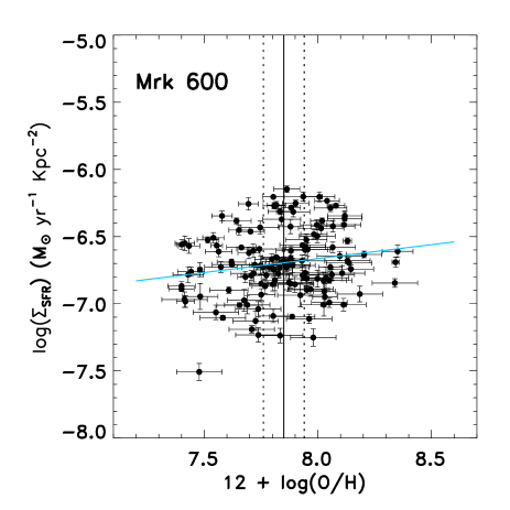
Figure 15: Relation between the star-formation rate Log($\Sigma_{SFR}$) and oxygen abundance 12 + log(O/H) at spaxel scales. The cyan line represents the linear fit to this relation. The integrated 12 + log(O/H) = 7.84$\pm$0.08 and 7.85$\pm$0.09 obtained for UM 461 and Mrk 600 are represented by the vertical solid lines, while the errors at the 1$\sigma$ level are shown as dotted lines.

Mrk 600. In Figure 15 (right panel) we observe a marginal gradient of increasing 12 + log(O/H) abundance and SFR, indicating that parcels of gas with higher metallicity are the locus of stronger star-forming activity than those found in low metallicity environments. However, the Pearson’s correlation coefficient between these two quantities is $\sim$0.2. The critical value for the two tailed non-directional test (0.02 significance) exceeds the Pearson’s correlation coefficient, supporting the hypothesis that the variables are not linearly correlated. We discard infalling metal-poor gas as the trigger for the ongoing starbursts in Mrk 600, since the ISM is chemically homogeneous as seen in Section 4.1. Interestingly, the 12 + log(O/H) map based on R23 shows higher values in the area in between the resolved shells in region no. 1 (see Figure 12). Consequently, there may have been an outflow of oxygen-enriched gas due to SNe. However, we cannot draw firm conclusions on this because no direct estimations of abundances were obtained.

In summary, the dispersion in the Log($\Sigma_{SFR}$) versus 12 + log(O/H) relation, at spaxel scales, for both galaxies is relatively high reflecting their star-formation histories. Given that dwarfs galaxies have shallow potential wells, both the ejection of metal rich material and accretion/interactions have a huge impact on their evolution. However, the current burst in UM 461 is unlikely to diminish its metal content, given that star-formation is inefficient at driving outflows. Therefore, an additional mechanism, such as cold accretion (Keres̆ et al., 2005) of metal-poor gas, must be at work in order to explain its observed properties and morphology.

4.4 Relationship between neutral and ionised gas

H i is highly sensitive to interactions even with minor satellite galaxies (Martínez-Delgado et al., 2009; Scott et al., 2014) while H i kinematic and morphological perturbations from major interactions can remain detectable for between 0.4 and 0.7 Gyr following a tidal interaction (e.g. Holwerda et al., 2011). UM 461 (M_HI = 1.71 $\times$ 10⁸ M_⊙; van Zee, Skillman & Salzer, 1998) has a near neighbour, UM 462, which is projected $\sim$17 arcmin (62 kpc) to the SE, with a $\Delta$ V_optical of only 18 km s^-1. A $\sim$ 6 arcmin (22 kpc) H i tail seen extending SE of UM 461 toward UM 462 in a VLA D–array H i map was originally interpreted as evidence of a recent tidal interaction between the pair (Taylor et al., 1995, their figure 8a). However, subsequent higher resolution VLA B and C–array H i mapping of UM 461 by van Zee, Skillman & Salzer (1998) failed to detect this tail, with those authors arguing the earlier apparent H i tail was probably an artefact produced by solar interference. Further evidence against a recent interaction between the pair comes from the regular H i  morphology and velocity field for UM 462 (van Zee, Skillman & Salzer, 1998, their figure 10). Additionally, James, Tsamis & Barlow (2010) found no evidence for significant nitrogen or oxygen variations across UM 462 at the 0.2 dex level. This result shows that from a chemical point of view, if there has been a recent interaction, it is not currently producing significant metallicity deviations or gradients in UM 462 at large scales.

While the van Zee, Skillman & Salzer (1998) H i velocity field for UM 461 (their figure 9d) shows an overall rotation pattern with a NW–SE rotation axis, it also reveals a strong asymmetric warp at velocities below 1040 km s^-1 projected S and SW of GH iiR no. 1. This highly warped region is referred to hereafter as the “disturbed H i region”. The faint broad optical SW tail seen in Figure 1 is projected at the western end of the disturbed H i region. At the eastern end of the disturbed H i region, directly S of the GH iiR no. 1 is the location of the anomalously metal-poor gas clump (Figs. 7). The v_r(H$\alpha$) minimum of $\sim$ 995 km s^-1 (Figure 9) is offset slightly further to the SW, but still within the disturbed H i region. The highest resolution (van Zee, Skillman & Salzer, 1998) H i map ($\sim$ 5 arcsec resolution) also shows the SW side of the H i disk is asymmetrically extended into the disturbed H i region. The combination of the disturbed H i region’s properties and the VIMOS-IFU data are consistent with the recent infall from the SW of a low mass metal-poor dwarf or H i cloud into the region now exhibiting the lowest metallicity, and localised perturbed neutral and ionized gas kinematics. We may be observing the impact of an event similar to that in CIG 85, where it is proposed that a small dwarf is in the process of being subsumed into a larger galaxy (Sengupta et al., 2012). We note that the faint broad optical tail in CIG 85 is attributed to the interaction (possibly multiple times) with a minor satellite. DDO 68 is another low metallicity dwarf galaxy with evidence of the recent accretion of a smaller satellite galaxy (Annibali et al., 2016; Sacchi et al., 2016).

In the case of Mrk 600, we did not find evidence of optical companions using NED. However, Noeske et al. (2005) suggest that the distribution of the star-forming knots in this galaxy may be the result of an ongoing or recent interaction. Noeske et al. argue that the U–B colours of -0.64, -0.72 and -0.86 of our regions no. 1 and no.2 and their region c, respectively, suggest propagating star-formation activity, while the colours of the underlying stellar component are indicative of a population of several Gyr old. However, they failed to detect an optical or near-IR counterpart to H i companion detected $\sim$ 1.25 arcmin SW of Mrk 600 by Taylor, Brinks & Skillman (1993) in their VLA D–array H i map. The companion’s reported M(H i) was 2.2 $\times$ 10⁷ M_⊙, i.e. $\sim$ 10% of the Mrk 600 M(H i), and it has a maximum column density of $\sim$1.5 $\times$ 10²⁰ atoms cm^-2 (Taylor, Brinks & Skillman, 1993). Nevertheless, the higher resolution VLA C–array H i map (Taylor et al., 1994) does not show a separate structure at the position of the preciously reported H i companion. The velocity field from VLA C–array observations for Mrk 600 revealed an overall, although rather irregular, H i rotation patten. If future H i observations confirm the H i companion this will indicate Mrk  600 is at an earlier stage of accreting a H i cloud with a significant mass.

4.5 Gas metallicity

Minor mergers or interactions could potentially provide a supply of infalling gas and the energy transfer to drive the internal motions of the parent galaxy. In this Section we will analyse this scenario in the context of the chemical evolution of UM 461 and Mrk 600. In a closed box model, the gas metal mass fraction Z (Schmidt, 1963; Searle & Sargent, 1972) is determined entirely by the yield ($y$) and gas fraction $f_{gas}$ = M_gas/(M_gas+M_stars) as

$$Z_{gas}=y\times ln(f_{gas}^{-1}).$$ (5)

If we express Z_gas in terms of the oxygen abundance we obtain:

$$12+log(O/H)=12+log(y_{O}/11.728)+log(ln(f_{gas}^{-1})),$$ (6)

where $y_{O}$ is the oxygen yield by mass and 11.728 is the factor to convert abundance by mass to abundance by number (Lee et al., 2006). Here, we consider M_gas = 1.24$\times$M_HI and the true yield log($y_{O}$) = -2.4 (Dalcanton, 2007). Therefore, we find that the measured oxygen abundance in UM 461 is $\Delta$(O/H) $\sim$ 0.38 dex lower than the expected value assuming a closed box model, while in Mrk 600 the oxygen abundance is $\Delta$(O/H) $\sim$ 0.07 dex higher. In terms of the effective yield $y_{eff}$ = Z_gas/ln($f_{gas}^{-1}$) (Z_gas = 12$\times$O/H), we found that log($y_{eff}$) = -2.77 and -2.32 for UM 461 and Mrk 600, respectively. In Figure 16 we show 12 + log(O/H) as a function of the gas fraction assuming a closed box model. The data points, in the same Figure, correspond to the measured values of UM 461 and Mrk 600. Note that, in the case of Mrk 600, if we assume a true yield $y_{O}$=0.01 (Tremonti et al., 2004), the data point is well explained, within the uncertainties, by the closed box model. However, the effective yield of UM 461 remains lower than the closed box model when we use either true yield prescription.

It is assumed that deviations from the closed box model indicate the presence of an outflow and/or inflow. In principle, we cannot rule out any of those mechanisms to decrease the effective yield found in UM 461 and the slightly higher yield in Mrk 600. However, and according to our previous analysis, Mrk 600 is currently less affected by outflows or inflows, which makes it well explained by a closed box model. Mrk 600 also presents a flat metallicity gradient within the uncertainties. In the case of UM 461, the low metallicity region, with 12 + log(O/H) $\lesssim$ 7.6, could be the result of inflow of metal-poor gas. According to Thuan et al. (2016), the deviations in the effective yields can be understood as a gas outflow, in which a high fraction of metal-enriched gas is lost, and/or inflow of metal-poor gas in objects where $y_{eff}\lesssim y_{true}$ and a relatively metal-free H i envelope for objects with $y_{eff}\gtrsim y_{true}$. Therefore, the deviation from the closed-box model in UM 461 can be explained as the result of the competing effects of starburst driven-outflows (e.g. Tremonti et al., 2004) and the inflow of metal-poor gas. However, the latter is the most likely factor to explain the low effective yields observed in UM 461, because starburst driven-outflows are unlikely to be effective in removing large amounts of gas from the disk in low-mass galaxies (e.g. Dalcanton, 2007), as discussed in Section 4.3. In this scenario, during the infall the oxygen abundance is reduced due to dilution of the pre-existing gas, without affecting the log(N/O) ratio, followed by the evolution of the system towards the closed-box relation (Köppen & Hensler, 2005).

Figure 16: Relation between 12 + log(O/H) as function of gas fraction $f_{gas}$ assuming a closed-box model assuming a true yield $y_{O}$ = 0.004 (solid line; Dalcanton, 2007) and $y_{O}$ = 0.01 (dashed line; Tremonti et al., 2004), typical oxygen yields for star-forming galaxies. Data points correspond to our measured values for UM 461 and Mrk 600.

The idea of an infall of pristine gas is unlikely to explain the effective yield of UM 461 because this infalling gas would increase its value significantly (Thuan et al., 2016). Alternatively, based on its high H i mass, the infall of metal-poor clouds ($\sim$10⁷M_⊙; Verbeke et al., 2014) towards the centre could produce the observed low metallicity region in UM 461. H i clouds have previously been found in the surroundings of some BCD galaxies (e.g. Thuan, Hibbard & Lévrier, 2004; Lelli, Verheijen & Fraternali, 2014). It seems that the H i companion to Mrk 600, if it really exists, has not yet been accreted into the galactic disk and we speculate that it would available to fuel a future starburst episodes and produce temporary metallicity and ionized gas kinematic inhomogeneities in the galaxy’s disk.

If UM 461 had been tidally disrupted due to an interaction(s) with UM 462, this may have promoted an efficient flattening of the metallicity gradient and dilution by low-metallicity gas infalling into the galaxy centre. Interestingly, the difference in oxygen abundance between UM 461 (7.84 dex; this work) and UM 462 (8.03 dex; James, Tsamis & Barlow, 2010) is 0.19 dex. This argues in favour of a coeval evolution of this pair. In fact, the current star-formation episodes in both galaxies are very young, not older than a few Myr with most of their underlying stellar populations formed $\sim$1 Gyr ago (Lagos et al., 2011). See Lagos et al. (2011) and Vanzi (2003) for a detailed study of the star cluster population in UM 461 and UM 462, respectively. However, the formation process of cometary galaxies near and far is unclear and different mechanisms may be at work during the evolution of those systems, i.e., propagating star-formation in local XMP BCDs (Papaderos et al., 2008), infall of metal-poor gas (e.g. Ekta & Chengalur, 2010; Verbeke et al., 2014) and interactions (e.g. Noeske et al., 2001; Pustilnik et al., 2001). If the accretion/inflow of gas is the main mechanism to trigger star-formation in cometary-like galaxies, this implies that both galaxies, in this study, are at different evolutionary stages.

By using IFU spectroscopy we have been able to investigate the chemical homogeneity in star-forming dwarf galaxies (e.g. Lagos & Papaderos, 2013; Lagos et al., 2014, 2016), obtaining precise abundance determinations in a sample of objects with clear detections of [O iii]$\lambda$4363 line emission. The detection of chemical inhomogeneities in XMP BCDs using the direct method, likely produced by the infall of metal-poor gas-clouds onto the ISM disc, is a key component for the study of the chemical evolution of those systems. Motivated by these results, we will explore with future IFU and H i observations the relations among various spatially resolved quantities (e.g. star-formation, kinematics, abundances, etc). This should give us insight into whether the infall of metal-poor gas-clouds is responsible for the detected low metallicity regions in some of those systems.

5 Summary and Conclusions

In this paper, we have analysed the ISM of the H ii/BCD galaxies UM 461 and Mrk 600 using VIMOS-IFU spectroscopy. The following points summarise the main results in this work:

• We obtained integrated oxygen abundances, using the direct method, 12 + log(O/H) = 7.84 and 7.85 for UM 461 and Mrk 600, respectively. We found a marginal difference between those integrated abundances and the ones found in the GH iiRs for both galaxies. Therefore, within the uncertainties we can consider that the oxygen abundance is fairly well mixed at large scales. In Figure 7 (left pannels) we showed the spaxel by spaxel 12 + log(O/H) maps of the galaxies using the direct method. We note that in the case of Mrk 600 the distribution of oxygen abundances from the spaxels can be fitted by a single Gaussian. While for UM 461 the distribution is well fitted by two Gaussians (see Figure 10). The mean values of both distributions agree with the integrated ones indicating that, at large scales, the ISM is chemically homogeneous. However, we found evidences of an off-centre low metallicity region, located in the southern part of region no. 1 in UM 461 . This area has an extension of $\sim$0.7 kpc and a mean value of 12 + log(O/H) $\sim$ 7.52. Whereas, Mrk 600, like other previously studied star-forming dwarf galaxies, is chemically homogeneous (see Lagos & Papaderos, 2013).

• We use BPT diagnostic diagrams to study the excitation conditions in both galaxies. We found that all points fall in the locus predicted by models of photo-ionization by young stars in H ii regions indicating that photoionization from stellar sources is the dominant excitation mechanism in UM 461 and Mrk 600.

• We checked the spatial variation of 12 + log(O/H) abundances in both galaxies using several calibrators (N2, O3N2, R23 and D2016), including the widely used HII–CHI–mistry code. The oxygen abundance maps N2 and O3N2 show spatial trends that are opposite to those shown by the direct method and R23. The shape of R23 agrees with the direct method, indicating only a small dependence on $U$ as compared with N2 and O3N2, where this dependence could be significant as proved in the literature (e.g. Kewley & Dopita, 2002). The D2016 maps do not correlate with any of the previous determinations. Applying the HII-CHI-mistry code (Pérez-Montero, 2014) to our spatially resolved data provides values for oxygen abundance consistent with the direct method only when the [O iii]$\lambda$4363 emission line is included as an input. Therefore, special attention must be paid when this method is used in studying the real spatial variation of abundances across galaxies.

• In both objects we find that the H${\alpha}$  velocity field (v_r) shows systemic motions. But in the case of UM 461 the combination of a region of disturbed H i  (van Zee, Skillman & Salzer, 1998) and our VIMOS-IFU velocity fields at the same location are consistent with the recent infall from the SW of a low mass metal-poor dwarf or H i cloud into the region now exhibiting the lowest metallicity and localised perturbed neutral and ionized gas kinematics.

• The dispersion in the Log($\Sigma_{SFR}$) versus 12 + log(O/H) relations in our galaxies is quite high and no correlation is found at spaxel scales. The effective yield for UM 461 is lower than predicted by the closed box model. This deviation from the model indicates the presence of inflows of non-pristine metal-poor gas which could explain the region of anomalously low metallicity in this galaxy. Whereas, the effective yield in Mrk 600 is well explained, within the uncertainties, by the closed-box model.

In summary, the spatially resolved properties of the galaxies are consistent with these systems being at different stages of accreting low metallicity H i gas-clouds to their stellar disks. Therefore, the detection of a low-metallicity region with 12 + log(O/H) $<$ 7.6 in the brightest H ii region of UM 461 indicate that the low-metallicity cloud has been “recently” accreted. Moreover, if the H i companion to Mrk 600 really exists, it has not yet been accreted into the galactic disk.

References

- Alloin et al. (1979) Alloin D., Collin-Souffrin S., Joly M., Vigroux J. M., 1979, A&A, 78, 200
- Annibali et al. (2016) Annibali F. et al., 2016, ApJ, 826, 27
- Baldwin, Phillips & Terlevich (1981) Baldwin, J. A., Phillips, M. M., Terlevich R. 1981, PASP, 93, 5
- Bournaud & Elmegreen (2009) Bournaud, F., Elmegreen, B. G. 2009, ApJ, 694, 158
- Bordalo & Telles (2011) Bordalo, V., Telles, E. 2011, ApJ, 735, 52
- Calzetti et al. (2007) Calzetti, D. et al. 2007, ApJ, 666, 870
- Cairós et al. (2001a) Cairós, L. M., Vílchez, J. M., González Pérez, J. N., Iglesias-Páramo, J., Caon, N. 2001a, ApJS, 133, 321
- Cairós et al. (2001b) Cairós, L. M., Caon, N., Vílchez, J. M., González-Pérez, J. N., Muñoz-Tuñón, C. 2001b, ApJS, 136, 393
- Cresci et al. (2010) Cresci, G., Mannucci, F., Maiolino, R., Marconi, A., Gnerucci, A., Magrini, L. 2010, Natur, 467, 811
- Cardelli, Clayton & Mathis (1989) Cardelli, J. A., Clayton, G. C., Mathis, J. S. 1989, ApJ, 345, 245
- Dalcanton (2007) Dalcanton J. J., 2007, ApJ, 658, 941
- Denicoló, Terlevich, & Terlevich (2002) Denicoló, G., Terlevich, R., & Terlevich, E. 2002, MNRAS, 330, 69
- Dekel et al. (2009) Dekel, A., Birnboim, Y., Engel, G., Freundlich, J., Goerdt, T., Mumcuoglu, M., Neistein, E., Pichon, C., Teyssier, R., Zinger, E. 2009, Natur, 457, 451
- Dekel & Birnboim (2006) Dekel, A., Birnboim, Y. 2006, MNRAS, 368, 2
- Díaz et al. (2000) Díaz, A. I., Castellanos, M., Terlevich, E., Luisa García-Vargas, M. 2000, MNRAS, 318, 462
- Dopita et al. (2016) Dopita, M. A., Kewley, L. J., Sutherland, R. S., Nicholls, D. C. 2016, Ap&SS, 361, 61
- Dors et al. (2011) Dors, O. L., Jr., Krabbe, A.; Hägele, G. F., Pérez-Montero, E. 2011, MNRAS, 415, 3616
- Edmunds & Pagel (1978) Edmunds M. G., Pagel B. E. J., 1978, MNRAS, 185, 77
- Ekta & Chengalur (2010) Ekta, B., Chengalur, J. N., 2010, MNRAS, 406, 1238
- Gil de Paz, Madore & Pevunova (2003) Gil de Paz, A., Madore, B. F., Pevunova, O. 2003, ApJS, 147, 29
- Guseva et al. (2011) Guseva, N. G., Izotov, Y. I., Stasińska, G., Fricke, K. J., Henkel, C., Papaderos, P. 2011, A&A, 529, 149
- Holwerda et al. (2011) Holwerda, B. W., Pirzkal, N., Cox, T. J., de Blok, W. J. G., Weniger, J., Bouchard, A., Blyth, S.-L., van der Heyden, K. J. 2011, MNRAS, 416, 2426
- James, Tsamis & Barlow (2010) James, B. L., Tsamis, Y. G., Barlow, M. J. 2010, MNRAS, 401, 759
- Janowiecki & Salzer (2014) Janowiecki, S., Salzer, J. J. 2014, ApJ, 793, 109
- Kehrig et al. (2016) Kehrig, C., Vílchez, J. M., Pérez-Montero, E., Iglesias-Páramo, J., Hernández-Fernández, J. D., Duarte Puertas, S., Brinchmann, J., Durret, F., Kunth, D. 2016, MNRAS, 459 2992
- Kennicutt (1998) Kennicutt, R. C. 1998 ARA&A, 36, 189
- Keres̆ et al. (2005) Keres̆, D., Katz, N., Weinberg, D. H., Davé, R. 2005, MNRAS, 363, 2
- Kewley & Dopita (2002) Kewley L. J., Dopita M. A., 2002, ApJS, 142, 35
- Kewley & Ellison (2008) Kewley L. J., Ellison S. L., 2008, ApJ, 681, 1183
- Kobulnicky et al. (1999) Kobulnicky, H. A., Kennicutt, R. C., Jr., Pizagno, J. L. 1999, ApJ, 514, 544
- Köppen & Hensler (2005) Köppen, J., Hensler, G. 2005, A&A, 434, 531
- Kumari, James & Irwin (2017) Kumari, N., James, B. L., Irwin M. J. 2017, arXiv:1706.02310
- Izotov & Thuan (1998) Izotov, Y. I., Thuan, T. X. 1998, ApJ, 500, 188
- Izotov & Thuan (1999) Izotov, Y. I., Thuan, T. X. 1999, ApJ, 511, 639
- Lagerholm et al. (2012) Lagerholm, C., Kuntschner, H., Cappellari, M., Krajnovic, D., McDermid, R. M., Rejkuba, M. 2012, A&A, 541, 82
- Lagos et al. (2007) Lagos, P., Telles E., Melnick J. 2007, A&A, 476, 89
- Lagos et al. (2009) Lagos, P., Telles, E., Muñoz-Tuñón, C., Carrasco, E. R., Cuisinier, F., Tenorio-Tagle G. 2009, AJ, 137, 5068
- Lagos et al. (2011) Lagos, P., Telles, E., Nigoche-Netro, A., Carrasco E. R. 2011, AJ, 142, 162
- Lagos et al. (2012) Lagos, P., Telles E., Nigoche-Netro A., Carrasco E. R. 2012, MNRAS, 427, 740
- Lagos & Papaderos (2013) Lagos, P., Papaderos, P. 2013, AdAst, 2013, 20
- Lagos et al. (2014) Lagos, P., Papaderos, P., Gomes, J. M., Smith, A. V., Vega, L. R. 2014, A&A, 569, 110
- Lagos et al. (2016) Lagos, P., Demarco, R., Papaderos, P., Telles, E., Nigoche-Netro, A., Humphrey, A., Roche, N., Gomes, J. M. 2016, MNRAS, 456, 1549
- Lebouteiller et al. (2009) Lebouteiller, V., Heap, S., Hubeny, I., Kunth, D. 2009, A&A, 494, 915
- Lee et al. (2006) Lee, H., Skillman, E. D., Cannon, J. M., Jackson, D. C., Gehrz, R. D., Polomski, E. F., Woodward, C. E. 2006, ApJ, 647, 970
- Le Févre et al. (2003) Le Févre, O., et al. 2003, SPIE, 4841, 1670
- Lelli, Verheijen & Fraternali (2014) Lelli, F., Verheijen, M., Fraternali, F. 2014, MNRAS, 445, 1694
- Loose & Thuan (1986) Loose, H.-H., Thuan, T. X. 1986, ApJ, 309, 59
- Martínez-Delgado et al. (2009) Martínez-Delgado, D., Pohlen, M., Gabany, R.,J., Majewski, S.,R., Peñarrubia, J., Palma, C. 2009, ApJ, 692, 955
- Masegosa, Moles & Campos-Aguilar (1994) Masegosa, J., Moles, M., Campos-Aguilar, A. 1994, ApJ, 420, 576
- Monreal-Ibero, Walsh & Vílchez (2012) Monreal-Ibero, A., Walsh, J. R., Vílchez, J. M. 2012, A&A, 544, 60
- Moustakas & Kennicutt (2006) Moustakas, J., Kennicutt, R. C. Jr. 2006, ApJS, 164, 81
- Noeske et al. (2001) Noeske, K. G., Iglesias-Páramo, J., Vílchez, J. M., Papaderos, P., Fricke, K. J. 2001, A&A, 371, 806
- Noeske et al. (2005) Noeske, K. G., Papaderos, P., Cairós, L. M., Fricke, K. J. 2005, A&A, 429, 115
- Osterbrock & Ferland (2006) Osterbrock, D. E., Ferland, G. J. 2006, Astrophysics of gaseous nebulae and active galactic nuclei, 2nd. edn. (Sausalito, CA: University Science Books)
- Olmo-García et al. (2017) Olmo-García, A., Sánchez Almeida, J., Muñoz-Tuñón, C., Filho, M. E., Elmegreen, B. G., Elmegreen, D. M., Pérez-Montero, E., Méndez-Abreu, J. 2017, ApJ, 834, 181O
- Papaderos et al. (2008) Papaderos, P., Guseva, N. G., Izotov, Y. I., Fricke, K. J. 2008, A&A, 491, 113
- Pettini & Pagel (2004) Pettini, M., Pagel, B. E. J. 2004, MNRAS, 348, 59
- Pérez-Montero & Díaz (2003) Pérez-Montero, E., Díaz, A. I. 2003, MNRAS, 346, 105
- Pérez-Montero et al. (2011) Pérez-Montero, E., Vílchez, J. M., Cedrés, B., Hägele, G. F., Mollá, M., Kehrig, C., Díaz, A. I., García-Benito, R., Martín-Gordón, D. 2011, A&A, 532, 141
- Pérez-Montero (2014) Pérez-Montero 2014, MNRAS, 441, 2663
- Pustilnik et al. (2001) Pustilnik, S. A., Kniazev, A. Y., Lipovetsky, V. A., Ugryumov, A. V. 2001, A&A, 373, 24
- Sacchi et al. (2016) Sacchi E. et al., 2016, ApJ, 830, 3
- Sánchez Almeida et al. (2014) Sánchez Almeida, J., Morales-Luis, A. B., Muñoz-Tunón, C., Elmegreen, D. M., Elmegreen, B. G., Méndez-Abreu, J. 2014, ApJ, 783, 45
- Sánchez Almeida et al. (2015) Sánchez Almeida, J., Elmegreen, B. G., Muñoz-Tuñón, C., Elmegreen, D. M., Pérez-Montero, E., Amorín, R., Filho, M. E., Ascasibar, Y., Papaderos, P., Vílchez, J. M. 2015, ApJ, 810, 15
- Sánchez Almeida et al. (2016) Sánchez Almeida, J., Pérez-Montero, E., Morales-Luis, A. B., Muñoz-Tuñón, C., García-Benito, R., Nuza, S. E., Kitaura, F. S. 2016, ApJ, 819, 110
- Sampaio Carvalho (2013) Sampaio Carvalho, M. 2013, Cinemática das Galáxias HII UM 461 e CTS 1020, Master’s thesis, UESC, BA.
- Scott et al. (2014) Scott, T., C., Sengupta, C., Verdes Montenegro, L., Bosma, A., Athanassoula, E., Sulentic, J., Espada, D., Yun, M.,S., Argudo-Fernández, M. 2014 A&A, 567,56
- Schlafly & Finkbeiner (2011) Schlafly, E. F., Finkbeiner, D. P. 2011, ApJ, 737, 103
- Searle & Sargent (1972) Searle, L., Sargent, W. L. W. 1972, ApJ, 173, 25
- Sengupta et al. (2012) Sengupta, C., Scott, T. C., Verdes Montenegro, L., Bosma, A., Verley, S., Vílchez, J. M., Durbala, A., Fernández Lorenzo, M., Espada, D., Yun, M. S., Athanassoula, E., Sulentic, J., Portas, A. 2012, A& A, 546, 95
- Schmidt (1963) Schmidt, M. 1963, ApJ, 137, 758
- Silich & Tenorio-Tagle (2001) Silich, S., Tenorio-Tagle, G. 2001, ApJ, 552, 91
- Smoker et al. (2000) Smoker, J. V., Davies, R. D., Axon, D. J., Hummel, E. 2000, A&A, 361, 19
- Straughn et al. (2006) Straughn, A. N., Cohen, S. H., Ryan, R. E., et al. 2006, ApJ, 639, 724
- Taylor, Brinks & Skillman (1993) Taylor, C., Brinks, E., Skillman, E. D. 1993, AJ, 105, 128
- Taylor et al. (1994) Taylor, C. L., Brinks, E., Pogge, R. W., Skillman, E. D. 1994, AJ, 107, 971
- Taylor et al. (1995) Taylor, C. L., Brinks, E., Grashuis, R. M., Skillman, E. D. 1995, ApJS, 99, 427
- Telles & Terlevich (1997) Telles, E., Terlevich, R. 1997, MNRAS, 286, 183
- Thuan, Hibbard & Lévrier (2004) Thuan, T. X., Hibbard, J. E., Lévrier, F. 2004, AJ, 128, 617
- Thuan et al. (2016) Thuan, T. X., Goehring, K. M., Hibbard, J. E., Izotov, Y. I., Hunt, L. K. 2016, MNRAS, 463, 4268
- Tolstoy, Hill & Tosi (2009) Tolstoy, Hill, Tosi 2009, ARA&A, 47, 371
- Tremonti et al. (2004) Tremonti, C. A., Heckman, T. M., Kauffmann, G., Brinchmann, J., Charlot, S., et al. 2004, ApJ, 613, 898
- van Zee, Skillman & Salzer (1998) van Zee, L., Skillman, E. D., Salzer, J. J. 1998, AJ, 116, 1186
- van Zee & Haynes (2006) van Zee, L., Haynes, M. P. 2006, ApJ, 636, 214
- van den Bergh et al. (1996) van den Bergh, S., Abraham, R. G., Ellis, R. S., et al. 1996, AJ, 112, 359
- Vanzi (2003) Vanzi, L. 2003, A&A, 408, 523
- Verbeke et al. (2014) Verbeke, R., De Rijcke, S., Koleva, M., Cloet-Osselaer, A., Vandenbroucke, B., Schroyen, J. 2014, MNRAS, 442, 1830
- Veilleux, Cecil & Bland-Hawthorn (2005) Veilleux, S., Cecil, G., Bland-Hawthorn, J. 2005, ARA&A, 43, 769
- Zhao, Gao & Gu (2013) Zhao, Y., Gao, Y., Gu, Q. 2013, ApJ, 764, 44
- Walsh & Roy (1990) Walsh J. R., Roy J. R., 1990, ESO Conf., 34, 95
- Windhorst et al. (2006) Windhorst, R. A., Cohen, S. H., Straughn, A. N., et al. 2006, New Astron. Rev., 50, 821