From elliptic multiple zeta values
to modular graph functions:
open and closed strings at one loop

1 Introduction

Modular graph functions are building blocks for one-loop scattering amplitudes in closed-string theories at the one-loop level. They have been thoroughly investigated by D’Hoker, Green, Vanhove and other authors during the last couple of years [1, 2, 3, 4, 5, 6, 7, 8, 9, 10, 11, 12, 13] and arise from Feynman graphs of certain conformal scalar fields on the torus. Each modular graph function depends on the modular parameter of the torus and its modular invariance is inherited from the underlying closed-string setup. While the computation of their asymptotic expansion is itself cumbersome, they exhibit a variety of mathematical structures: modular graph functions are related by a network of algebraic identities and related to holomorphic Eisenstein series by differential equations with respect to the modular parameter. Even more, they satisfy certain eigenvalue equations involving the modular invariant Laplace operator.

Most interestingly for the purpose of this article, however, a first connection between elliptic multiple polylogarithms (as defined in refs. [14, 15, 16]) and modular graph functions was established in ref. [6]: The latter were written as special values of infinite sums of single-valued multiple polylogarithms, and these infinite sums are proposed in the reference to be a single-valued analogue of elliptic multiple polylogarithms. This connection extends an observation made for genus-zero (tree-level) open- and closed-string amplitudes: closed-string tree amplitudes are conjectured to be obtained by acting with the so-called single-valued projection on the multiple zeta values appearing in their open-string counterparts [17, 18, 19]. The single-valued projection maps generic multiple zeta values to those instances which descend from single-valued polylogarithms at genus zero [20, 21].

At genus one (one-loop level), Enriquez’s elliptic multiple zeta values [22] were shown to capture the low-energy expansion of the open superstring [23, 24, 25]. The results of [6] suggest to expect that modular graph functions are single-valued versions of Enriquez’s elliptic multiple zeta values. However, the precise matching and thus the relation between open- and closed-string results at one-loop level is an open problem: First, the closed-string [6] and open-string literature [23, 24, 25] use different notions of elliptic polylogarithms. Second, the dependence of modular graph functions and elliptic multiple zeta values on the modular parameters of the respective genus-one surface is realized in rather different languages.

In the current article we are going to bridge the leftover gap between one-loop open- and closed-string amplitudes before integration over the respective modular parameters. We propose a setup which allows to relate certain building blocks of open-string amplitudes with modular graph functions. This accumulates evidence for a conjectural elliptic generalization of the single-valued projection known from genus zero. Simultaneously, this leads to a conjectural formalism to explicitly construct modular graph functions starting from open-string quantities. The results thus obtained pass a variety of consistency checks and match previous partial expressions.

The main idea is to define open-string graph functions within an abelian version of one-loop open-string amplitudes. Despite the fact that the permissible string spectrum of Type-I open-superstring theory does not contain an abelian gauge boson [26], we will consider a kinematical building block of the putative amplitude, which is non-trivial and well-defined for auxiliary abelian particles. In order to implement the abelian character of the auxiliary particles, the integration regions for open-string punctures are symmetrized in a convenient manner. The symmetrized open-string integrals of the abelian setup are the key to lining up the properties of the open-string genus-one Green function with its closed-string counterpart. In particular, the graphical organization of the low-energy expansion of open- and closed-string amplitudes in terms of open-string and modular graph functions agrees, which allows for direct comparison between constituents. This includes a matching of the respective differential equations in the modular parameter on the open- and closed-string side.

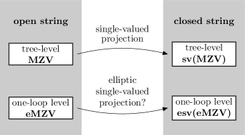
Figure 1: Context of a tentative generalization “esv” of the single-valued projection to genus one.

1.1 Summary of results

The notion of a single-valued projection applies to a variety of situations [27]. The most common examples are multiple zeta values (MZVs),

$$\zeta_{n_{1},n_{2},\ldots,n_{r}}:=\sum_{0<k_{1}<k_{2}<\ldots<k_{r}}^{\infty}k_{1}^{-n_{1}}k_{2}^{-n_{2}}\ldots k_{r}^{-n_{r}}\ ,\ \ \ \ n_{i}\in\mathbb{N}^{+},\,\,n_{r}\geq 2\,,$$ (1.1)

of weight $n_{1}{+}n_{2}{+}\ldots{+}n_{r}$ and depth $r$, which can be represented as multiple polylogarithms evaluated at unit argument. In contrast, single-valued MZVs descend from single-valued multiple polylogarithms at unit argument [21]. As explained in the reference, the single-valued projection formally denoted as

$$\text{sv}(\operatorname{\zeta}_{n_{1},\ldots,n_{r}})=\operatorname{\zeta}^{\text{sv}}_{n_{1},\ldots,n_{r}}$$ (1.2)

maps generic MZVs (1.1) to their single-valued counterparts, e.g.

$$\zeta^{\text{sv}}_{2k} =0\,,\quad\ \ \zeta^{\text{sv}}_{2k+1}=2\zeta_{2k+1}\,,\quad k\in\mathbb{N}^{+}$$ (1.3)

$$\zeta^{\text{sv}}_{3,5} =-10\zeta_{3}\zeta_{5}\,,\quad\ \ \zeta^{\text{sv}}_{3,5,3}=2\zeta_{3,5,3}-2\zeta_{3}\zeta_{3,5}-10\zeta_{3}^{2}\zeta_{5}\,.$$

As will be reviewed in the next section, the single-valued projection of MZVs appears naturally in relating tree-level scattering amplitudes of open and closed strings: the single-valued map acts on the MZVs arising in the low-energy expansion of open-string disk integrals and yields the closed-string integral over a punctured sphere. Correspondingly, it would be desirable to identify a similar map called “esv” for the elliptic version of multiple zeta values $\omega$ (to be defined and discussed below)

$$\text{esv}(\operatorname{\omega}({n_{1},\ldots,n_{r}\hskip 1.0pt|\hskip 1.0pt\tau}))=\operatorname{\omega}^{\text{esv}}(n_{1},\ldots,n_{r}\hskip 1.0pt|\hskip 1.0pt\tau)$$ (1.4)

at the one-loop level. As will be shown in this article, one-loop open- and closed-string amplitudes – expressed as open-string and modular graph functions, respectively – can be taken as a starting point to propose an analogous single-valued projection of elliptic multiple zeta values (eMZVs), see figure 1. Accordingly, we are going to describe operations on open-string graph functions in suitable presentations, which conjecturally yield modular graph functions as their one-loop closed-string counterparts,

$$\text{esv}\left(\begin{array}[]{c}\textrm{open-string}\\ \textrm{graph function}\end{array}\right)=\left(\begin{array}[]{c}\textrm{closed-string mo-}\\ \textrm{dular graph function}\end{array}\right)\,.$$ (1.5)

As will be detailed below, the present formulation of the operations in esv is in general ill-defined, as it is not compatible with the shuffle multiplication law of certain iterated Eisenstein integrals. Still, the conjecture eq. (1.5) is well defined for the leading terms in the expansion of both sides around the cusp, and for the complete expansions of modular graph functions that evaluate to non-holomorphic Eisenstein series. Moreover, it is highly non-trivial that there seem to exist rather natural representations of the open-string input, which yield modular graph functions beyond non-holomorphic Eisenstein series under the map esv.

We will provide examples of the correspondence eq. (1.5), up to and including the seventh subleading order in the low-energy expansion. In particular, starting from eq. (1.5), we will establish a new connection between building blocks of open- and closed-string four-point amplitudes

$$\text{esv}\ M^{\rm open}_{4}(s_{ij}\hskip 1.0pt|\hskip 1.0pt-\tfrac{1}{\tau})=M_{4}^{\textrm{closed}}(s_{ij}\hskip 1.0pt|\hskip 1.0pt\tau)\ .$$ (1.6)

These functions of the modular parameters $\tau$ of the underlying Riemann surfaces result from integrating over the open- and closed-string punctures and yield the respective building blocks for amplitudes upon integration over $\tau$. We will furthermore provide evidence that the planar open-string integral on the left-hand side can be replaced by any of its non-planar counterparts, irrespective on how the four state insertions are distributed over the boundaries of the worldsheet.

It is important to mention that a way to produce a single-valued projection of eMZVs (and therefore of open-string graph functions) already exists in the literature: it is based on their representation in terms of iterated integrals of Eisenstein series (as will be explained later in section 2), followed by the construction given in Francis Brown’s papers [28] and [29]. Brown’s construction maps iterated integrals of Eisenstein series to certain modular-invariant real-analytic functions whose coefficients are single-valued MZVs. So far, however, it remains conjectural that modular graph functions are contained in the image of this elliptic single-valued projection. We postpone the investigation of the relation between our single-valued projection and Brown’s map to a sequel of the present work.

1.2 Outline

Several techniques and previous results entering the construction of this work are reviewed in section 2. First, a short review is given on the single-valued projection in the context of regular multiple zeta values, which appear at string tree level. Second, $A$- and $B$-cycle versions of eMZVs will be reviewed. As it will turn out, modular transformations are facilitated by representing $A$- and $B$-cycle elliptic multiple zeta values in the language of iterated integrals over Eisenstein series. Modular graph functions including some of their properties are introduced briefly.

In section 3, open-string graph functions are introduced. While starting from the so-called $A$-cycle graph functions, it will turn out that finally $B$-cycle functions are the objects necessary for the construction of modular graph functions.

Once open-string graph functions are properly introduced, the comparison with modular graph functions can happen, and it is presented in section 4. Using several examples, we will finally arrive at a set of rules relating open-string graph functions to modular graph functions. This is first of all done at the level of the relations and differential equations in the modular parameter satisfied by the respective graph functions, see subsection 4.1 and subsection 4.2. From the resulting conjectures, modular graph functions can be obtained from their open-string counterparts up to integration constants. Moreover, since eMZVs are related to what is believed to be a single-valued version thereof in subsection 4.3, the construction is believed to constitute a representation of an elliptic single-valued projection. Still, in view of the issues with the shuffle multiplication of iterated Eisenstein integrals detailed in subsection 4.3, parts of the operations in the tentative elliptic single-valued projection await a reformulation in the future.

Finally, non-planar analogues of the above open-string graph functions are introduced in section 5, generalizing our main result eq. (1.6) to admit the integrals for arbitrary non-planar four-point open-string amplitudes on the left-hand side.

Various details and examples can be found in the appendices. In appendix A we provide a table allowing to translate our graphical notation to different notations for modular graph functions appearing in earlier articles on the subject.

2 Basics

2.1 Single-valued projection at tree level

In this section, we provide a brief review of the tree-level relations between open- and closed-string amplitudes and identify them as the single-valued projection in eq. (1.2).

Tree amplitudes among $n$ massless open-string states can be represented by moduli-space integrals over punctured disks accompanied by partial amplitudes of the Yang–Mills field theory [30, 31]. The moduli-space integrals read

$$Z(\rho(1,2,\ldots,n)\hskip 1.0pt|\hskip 1.0pt\sigma(1,2,\ldots,n)):=\!\!\!\!\!\!\!\int\limits_{D(\rho(1),\rho(2),\ldots,\rho(n))}\!\!{\mathrm{d}z_{1}\,\mathrm{d}z_{2}\cdots\mathrm{d}z_{n}\over{\rm vol}(\text{SL}(2,\mathbb{R}))}\frac{\prod_{i<j}^{n}|z_{ij}|^{-s_{ij}}}{\sigma(z_{12}z_{23}\ldots z_{n-1,n}z_{n,1})}\,,$$ (2.1)

where $z_{i}$ are the positions of the punctures on the boundary of a disk. The integral $Z(\cdot\hskip 1.0pt|\hskip 1.0pt\cdot)$ in eq. (2.1) is labeled by two permutations $\sigma,\rho\in S_{n}$ of the external legs $1,2,\ldots,n$ which govern the cyclic product of $z_{ij}:=z_{i}-z_{j}$ in the denominator (with $\sigma(z_{ij})=z_{\sigma(i),\sigma(j)}$) and the integration domains

$$D(1,2,\ldots,n)=\{(z_{1},z_{2},\ldots,z_{n})\in\mathbb{R}^{n},\ -\infty<z_{1}<z_{2}<\ldots<z_{n}<\infty\}\,.$$ (2.2)

The division by the inverse volume ${\rm vol}(\text{SL}(2,\mathbb{R}))$ of the conformal Killing group can be implemented by dropping any three integrations, fixing the respective positions such as $(z_{1},z_{{n-1}},z_{n})=(0,1,\infty)$, and inserting the compensating Jacobian $|z_{1,n-1}z_{1,n}z_{n-1,n}|$. Finally, the disk integrals eq. (2.1) depend on the lightlike momenta $k_{j}$ of the external states $j=1,2,\ldots,n$ subject to momentum conservation $\sum_{j=1}^{n}k_{j}=0$ through the dimensionless Mandelstam variables

$$s_{ij}=-\frac{\alpha^{\prime}}{2}\,\,k_{i}\cdot k_{j}$$ (2.3)

involving the inverse string tension $\alpha^{\prime}$.

Tree-level amplitudes among massless closed-string states, in turn, comprise moduli-space integrals over punctured spheres,

$$W(\rho(1,2,\ldots,n)\hskip 1.0pt|\hskip 1.0pt\sigma(1,2,\ldots,n)):=\pi^{3-n}\int\limits_{\mathbb{C}^{n}}{\mathrm{d}^{2}z_{1}\,\mathrm{d}^{2}z_{2}\cdots\mathrm{d}^{2}z_{n}\over{\rm vol}(\text{SL}(2,\mathbb{C}))}\frac{\prod_{i<j}^{n}|z_{ij}|^{-2s_{ij}}}{\sigma(z_{12}z_{23}\ldots z_{n,1})\ \rho(\bar{z}_{12}\bar{z}_{23}\ldots\bar{z}_{n,1})}\,,$$ (2.4)

where both permutations $\rho,\sigma\in S_{n}$ label a cyclic product of $z_{ij}$ or their complex conjugates. The inverse volume ${\rm vol}(\text{SL}(2,\mathbb{C}))$ suppresses three complex integrations and the normalization factor $\pi^{3-n}$ is chosen for later convenience.

The low-energy regime of string amplitudes is encoded in the Taylor expansion of the disk and sphere integrals around small values of the inverse string tension $\alpha^{\prime}$ and thus small values of the Mandelstam variables (2.3). The $w$’th order in the low-energy expansion beyond the respective field-theory amplitudes gives rise to MZVs eq. (1.1) of weight $w$ [33, 34], for instance

$$s_{12}Z(1,2,3,4\hskip 1.0pt|\hskip 1.0pt1,2,4,3) =\exp\Big{(}\sum_{n=2}^{\infty}\frac{\zeta_{n}}{n}\big{[}s_{12}^{n}+s_{23}^{n}-(s_{12}+s_{23})^{n}\big{]}\Big{)}$$ (2.5)

$$s_{12}W(1,2,3,4\hskip 1.0pt|\hskip 1.0pt1,2,4,3) =\exp\Big{(}2\sum_{k=1}^{\infty}\frac{\zeta_{2k+1}}{2k+1}\big{[}s_{12}^{2k+1}+s_{23}^{2k+1}-(s_{12}+s_{23})^{2k+1}\big{]}\Big{)}\,.$$ (2.6)

Generic examples of multiplicity $n\geq 5$ also involve MZVs of higher depth $r\geq 2$ [35, 17], and the explicit polynomial dependence on the Mandelstam invariants can for instance be computed via polylogarithm manipulations [31], the Drinfeld associator [42] or a Berends–Giele recursion for a putative effective field theory of bi-colored scalars [43]. A machine-readable form of such results is available for download on the website [44].

Closed-string integrals (2.4) can in principle be assembled from squares of open-string integrals (2.1) through the Kawai–Lewellen–Tye (KLT) relations [45]. However, the KLT formula obscures the cancellation of various MZVs from the open-string constituents: From the all-order conjectures of ref. [17], closed-string integrals (2.4) are expected to be single-valued open-string integrals [18, 19],

$$W(\rho(1,2,\ldots,n)\hskip 1.0pt|\hskip 1.0pt\sigma(1,2,\ldots,n))=\text{sv}\,Z(\rho(1,2,\ldots,n)\hskip 1.0pt|\hskip 1.0pt\sigma(1,2,\ldots,n))\,.$$ (2.7)

The MZVs in the image of the single-valued projection sv$(\ldots)$ are precisely the single-valued MZVs described in eqs. (1.2) and (1.3) above – in agreement with the four-point examples eqs. (2.5) and (2.6). As can be seen from eq. (2.7), the sv-projection trades the integration domain of the disk integral eq. (2.1) for an antiholomorphic cyclic denominator of a sphere integral (2.4).

2.2 $A$- and $B$-cycle eMZVs and iterated Eisenstein integrals

Several versions of eMZVs have been used in different contexts: when represented as special values of multiple elliptic polylogarithms (defined by Brown and Levin in [16]), they have made an appearance in the evaluation of the sunrise integral, see for instance [46, 47, 48, 49, 50, 51, 52, 53, 54, 55], while when represented as the coefficients of the elliptic associator (defined by Enriquez in [56]), they have made an appearance in the one-loop open-string amplitudes. The latter is the context that we consider in this article; therefore our conventions are inspired by the string-theory setup in refs. [23, 24, 25]. A further comprehensive reference on eMZVs is Matthes’s PhD thesis [57].

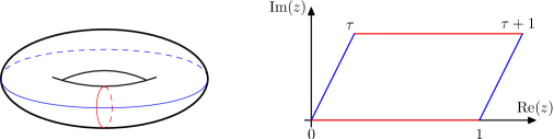
Figure 2: Parametrization of a torus as a lattice $\mathbb{C}/(\mathbb{Z}{+}\tau\mathbb{Z})$ with modular parameter $\tau$ in the upper half plane and complex coordinate $z\cong z{+}1\cong z{+}\tau$. The homology cycle drawn in red is mapped to the unit interval $(0,1)$ and referred to as the $A$-cycle. Accordingly, the second homology cycle mapped to the path from $0$ to $\tau$ is known as the $B$-cycle.

$A$-cycle eMZVs are defined as iterated integrals over the unit interval

$$\operatorname{\omega}_{A}(n_{1},n_{2},\ldots,n_{r}\hskip 1.0pt|\hskip 1.0pt\tau) :=\!\!\!\!\!\!\!\!\!\int\limits_{0\leq z_{1}\leq z_{2}\leq\ldots\leq z_{r}\leq 1}\!\!\!\!\!\!\!\!\!f^{(n_{1})}(z_{1},\tau)\,\mathrm{d}z_{1}\,f^{(n_{2})}(z_{2},\tau)\,\mathrm{d}z_{2}\,\ldots\,f^{(n_{r})}(z_{r},\tau)\,\mathrm{d}z_{r}\,,$$ (2.8)

where the integration path is taken to be on the real line. Using the parametrization of the torus in figure 2, the integration domain in eq. (2.8) corresponds to the $A$-cycle and justifies the term “$A$-cycle eMZVs”. Accordingly, iterated integrals along the $B$-cycle connecting the points $0$ and $\tau$ in figure 2 give rise to $B$-cycle eMZVs

$$\operatorname{\omega}_{B}(n_{1},n_{2},\ldots,n_{r}\hskip 1.0pt|\hskip 1.0pt\tau) :=\!\!\!\!\!\!\!\!\!\!\!\int\limits_{0\leq z_{1}\leq z_{2}\leq\ldots\leq z_{r}\leq\tau}\!\!\!\!\!\!\!\!\!\!\!f^{(n_{1})}(z_{1},\tau)\,\mathrm{d}z_{1}\,f^{(n_{2})}(z_{2},\tau)\,\mathrm{d}z_{2}\,\ldots\,f^{(n_{r})}(z_{r},\tau)\,\mathrm{d}z_{r}\,.$$ (2.9)

The doubly-periodic integration kernels $f^{(n)}$ in eqs. (2.8) and (2.9) are defined by their generating series [23, 24],

$$\exp\bigg{(}2\pi i\alpha\frac{\operatorname{Im}(z)}{\operatorname{Im}(\tau)}\bigg{)}\frac{\theta^{\prime}(0,\tau)\theta(z+\alpha,\tau)}{\theta(z,\tau)\theta(\alpha,\tau)}=\sum_{n=0}^{\infty}\alpha^{n-1}f^{(n)}(z,\tau)\,,$$ (2.10)

where $\theta(z,\tau)$ denotes the odd Jacobi theta function, and the simplest instances are $f^{(0)}(z,\tau)=1$ as well as $f^{(1)}(z,\tau)=\partial_{z}\log\theta(z,\tau)+2\pi i\frac{\operatorname{Im}(z)}{\operatorname{Im}(\tau)}$. We refer to the number $r$ of entries of eMZVs and the quantity $n_{1}+n_{2}+\ldots+n_{r}$ as their length and weight, respectively. Furthermore, the number of non-zero entries $n_{j}\neq 0$ of eMZVs will be referred to as their depth.

$B$-cycle eMZVs can be obtained from $A$-cycle eMZVs by the modular $S$-transformation, which sends $\tau\to-\frac{1}{\tau}$,

$$\operatorname{\omega}_{A}(n_{1},n_{2},\ldots,n_{r}\hskip 1.0pt|\hskip 1.0pt\!-\tfrac{1}{\tau})=\tau^{n_{1}+n_{2}+\ldots+n_{r}-r}\operatorname{\omega}_{B}(n_{1},n_{2},\ldots,n_{r}\hskip 1.0pt|\hskip 1.0pt\tau)\,.$$ (2.11)

Since the restriction of the kernels $f^{(n)}$ to the real line admits a Fourier-expansion in $q=\mathrm{e}^{2\pi i\tau}$ spelt out in subsection 3.3.3 of ref. [23], the same is true for $A$-cycle eMZVs in eq. (2.8), and one can prove that the coefficients are given by $\mathbb{Q}[(2\pi i)^{\pm 1}]$-linear combinations of MZVs [22].

By contrast, $B$-cycle eMZVs have the more complicated behavior near the cusp $\tau\to i\infty$ (or $q\to 0$) [22, 58],

$$\operatorname{\omega}_{B}(n_{1},n_{2},\ldots,n_{r}\hskip 1.0pt|\hskip 1.0pt\tau)=\sum_{l=1-n_{1}-\cdots-n_{r}}^{r}\!\!\!\tau^{l}\ \sum_{k=0}^{\infty}b_{k,l}(n_{1},n_{2},\ldots,n_{r})\,q^{k}\ ,\ \ \ \ \ \ n_{1},n_{r}\neq 1\ ,$$ (2.12)

where the coefficients $b_{k,l}(n_{1},n_{2},\ldots,n_{r})$ are $\mathbb{Q}[(2\pi i)^{\pm 1}]$-linear combinations of MZVs. In the resulting expansion for $S$-transformed $A$-cycle eMZVs

$$\operatorname{\omega}_{A}(n_{1},n_{2},\ldots,n_{r}\hskip 1.0pt|\hskip 1.0pt\!-\tfrac{1}{\tau})=\sum_{l=1-r}^{n_{1}+\cdots+n_{r}}(2\pi i\tau)^{l}\sum_{k=0}^{\infty}c_{k,l}(n_{1},n_{2},\ldots,n_{r})q^{k}\ ,\ \ \ \ \ \ n_{1},n_{r}\neq 1\ ,$$ (2.13)

it is crucial for later purposes to note that the coefficients $c_{k,l}(n_{1},n_{2},\ldots,n_{r})$ are $\mathbb{Q}$-linear (rather than $\mathbb{Q}[(2\pi i)^{\pm 1}]$-linear) combinations of MZVs. As will be proven in appendix C, all extra powers of $\pi$ can been absorbed into powers of $2\pi i\tau$ in eq. (2.13).

2.2.1 Elliptic iterated integrals

In the same way as MZVs descend from multiple polylogarithms at unit argument, $A$-cycle eMZVs defined in eq. (2.8) are special cases of elliptic iterated integrals subject to the recursive definition [23]

$$\operatorname{\Gamma}\left(\begin{smallmatrix}n_{1}&n_{2}&\ldots&n_{r}\\ a_{1}&a_{2}&\ldots&a_{r}\end{smallmatrix};z\hskip 1.0pt|\hskip 1.0pt\tau\right):=\int^{z}_{0}\mathrm{d}t\,f^{(n_{1})}(t-a_{1},\tau)\,\operatorname{\Gamma}\left(\begin{smallmatrix}n_{2}&\ldots&n_{r}\\ a_{2}&\ldots&a_{r}\end{smallmatrix};t\hskip 1.0pt|\hskip 1.0pt\tau\right)$$ (2.14)

with initial condition $\Gamma\,(;z\hskip 1.0pt|\hskip 1.0pt\tau)=1$, integration path along the real line and real upper limit $z$. Accordingly,

$$\operatorname{\omega}_{A}(n_{1},n_{2},\ldots,n_{r}\hskip 1.0pt|\hskip 1.0pt\tau)=\operatorname{\Gamma}\left(\begin{smallmatrix}n_{r}&\ldots&n_{2}&n_{1}\\ 0&\ldots&0&0\end{smallmatrix};1\hskip 1.0pt|\hskip 1.0pt\tau\right)\,.$$ (2.15)

The integrals defined in eq. (2.14) above are not homotopy invariant. However, as discussed in ref. [16] (see also subsection 3.1 of ref. [23]), every integral $\operatorname{\Gamma}\left(\begin{smallmatrix}n_{1}&n_{2}&\ldots&n_{r}\\ a_{1}&a_{2}&\ldots&a_{r}\end{smallmatrix};z\hskip 1.0pt|\hskip 1.0pt\tau\right)$ can be lifted to a homotopy invariant integral. Thus, despite the lack of homotopy invariance, various manipulations are still allowed for the integrals defined in eq. (2.14). In particular, as will become important for later computations, differential equations in $a_{i}$ acting on the iterated elliptic integrals defined in eq. (2.14) can be used to eliminate any additional occurrences of the argument $z$ on the left of the semicolon [23], for instance

$$\operatorname{\Gamma}\left(\begin{smallmatrix}n\\ z\end{smallmatrix};z\hskip 1.0pt|\hskip 1.0pt\tau\right) =(-1)^{n}\operatorname{\Gamma}\left(\begin{smallmatrix}n\\ 0\end{smallmatrix};z\hskip 1.0pt|\hskip 1.0pt\tau\right)$$ (2.16)

$$\operatorname{\Gamma}\left(\begin{smallmatrix}1&0&1\\ z&0&0\end{smallmatrix};z\hskip 1.0pt|\hskip 1.0pt\tau\right) =2\operatorname{\Gamma}\left(\begin{smallmatrix}0&0&2\\ 0&0&0\end{smallmatrix};z\hskip 1.0pt|\hskip 1.0pt\tau\right)+\operatorname{\Gamma}\left(\begin{smallmatrix}0&2&0\\ 0&0&0\end{smallmatrix};z\hskip 1.0pt|\hskip 1.0pt\tau\right)-2\operatorname{\Gamma}\left(\begin{smallmatrix}0&1&1\\ 0&0&0\end{smallmatrix};z\hskip 1.0pt|\hskip 1.0pt\tau\right)+\zeta_{2}\operatorname{\Gamma}\left(\begin{smallmatrix}0\\ 0\end{smallmatrix};z\hskip 1.0pt|\hskip 1.0pt\tau\right)\,.$$ (2.17)

2.2.2 Iterated Eisenstein integrals

Given that the differential equation in appendix C.2 allows to relate eMZVs to Eisenstein series, it is natural to represent them in terms of iterated integrals in $\tau$ (or $q=\mathrm{e}^{2\pi i\tau}$), see ref. [24] for the detailed formalism of iterated Eisenstein integrals,

$$\operatorname{\mathcal{E}}(k_{1},k_{2},\ldots,k_{r};\tau) :=2\pi i\int^{i\infty}_{\tau}\mathrm{d}\tau_{r}\ \frac{\operatorname{G}_{k_{r}}(\tau_{r})}{(2\pi i)^{k_{r}}}\operatorname{\mathcal{E}}(k_{1},k_{2},\ldots,k_{r-1};\tau_{r})$$

$$\phantom{:}=-\int^{q}_{0}\operatorname{\mathrm{dlog}}q_{r}\,\frac{\operatorname{G}_{k_{r}}(q_{r})}{(2\pi i)^{k_{r}}}\,\operatorname{\mathcal{E}}(k_{1},k_{2},\ldots,k_{r-1};q_{r})$$ (2.18)

$$\phantom{:}=(-1)^{r}\int\limits_{0\leq q_{1}\leq q_{2}\leq\ldots\leq q_{r}\leq q}\operatorname{\mathrm{dlog}}q_{1}\cdots\operatorname{\mathrm{dlog}}q_{r}\,\frac{\operatorname{G}_{k_{1}}(q_{1})}{(2\pi i)^{k_{1}}}\cdots\frac{\operatorname{G}_{k_{r}}(q_{r})}{(2\pi i)^{k_{r}}}\$$

$$\operatorname{\mathcal{E}_{0}}(k_{1},k_{2},\ldots,k_{r};\tau) :=2\pi i\int^{i\infty}_{\tau}\mathrm{d}\tau_{r}\ \frac{\operatorname{G}^{0}_{k_{r}}(\tau_{r})}{(2\pi i)^{k_{r}}}\operatorname{\mathcal{E}}(k_{1},k_{2},\ldots,k_{r-1};\tau_{r})$$

$$\phantom{:}=-\int^{q}_{0}\operatorname{\mathrm{dlog}}q_{r}\,\frac{\operatorname{G}^{0}_{k_{r}}(q_{r})}{(2\pi i)^{k_{r}}}\,\operatorname{\mathcal{E}_{0}}(k_{1},k_{2},\ldots,k_{r-1};q_{r})$$ (2.19)

$$\phantom{:}=(-1)^{r}\int\limits_{0\leq q_{1}\leq q_{2}\leq\ldots\leq q_{r}\leq q}\operatorname{\mathrm{dlog}}q_{1}\cdots\operatorname{\mathrm{dlog}}q_{r}\,\frac{\operatorname{G}^{0}_{k_{1}}(q_{1})}{(2\pi i)^{k_{1}}}\cdots\frac{\operatorname{G}^{0}_{k_{r}}(q_{r})}{(2\pi i)^{k_{r}}}\ .$$

The recursion starts with $\operatorname{\mathcal{E}}(;\tau)=\operatorname{\mathcal{E}_{0}}(;\tau)=1$, and the non-constant parts of Eisenstein series are defined as

$$\operatorname{G}^{0}_{2n}(\tau)=\operatorname{G}_{2n}(\tau)-2\operatorname{\zeta}_{2n}\,,\ \ \ \ \ \ \operatorname{G}_{0}(\tau)=\operatorname{G}^{0}_{0}(\tau)=-1\,$$ (2.20)

with $n\in\mathbb{N}^{+}$. Our conventions for Eisenstein series $\operatorname{G}_{k}$ are listed in appendix D.1, and we will interchangeably refer to the argument of $\operatorname{G}_{k}$, $\operatorname{G}^{0}_{k}$ and their iterated integrals by $\tau$ or $q$. For both $\operatorname{\mathcal{E}}(k_{1},k_{2},\ldots,k_{r};\tau)$ and $\operatorname{\mathcal{E}_{0}}(k_{1},k_{2},\ldots,k_{r};\tau)$ in eqs. (2.18) and (2.19), we will refer to the number of non-zero entries ($k_{j}\neq 0$) as the depth of the respective iterated Eisenstein integral (similar to the terminology for eMZVs).

Throughout this article, the endpoint divergences of the above integrals as $q_{1}\rightarrow 0$ are understood to be shuffle-regularized through the tangential-basepoint prescription described in ref. [59] with the net effect $\int^{q}_{0}\frac{\mathrm{d}q_{1}}{q_{1}}=\log q$. The iterated Eisenstein integrals $\operatorname{\mathcal{E}_{0}}(k_{1},\ldots,k_{r};q)$ with $k_{1}\neq 0$ do not need to be regularized and have the following Fourier-expansion (cf. eq. (4.62) of ref. [24]):

$$\operatorname{\mathcal{E}_{0}}(k_{1},0^{p_{1}-1},k_{2},0^{p_{2}-1},\ldots,k_{r},0^{p_{r}-1};q)=(-2)^{r}\bigg{(}\prod_{j=1}^{r}\frac{1}{(k_{j}-1)!}\bigg{)}$$ (2.21)

$$\ \ \ \ \ \ \ \times\sum_{m_{i},n_{i}=1}^{\infty}\frac{m_{1}^{k_{1}-1}m_{2}^{k_{2}-1}\ldots m_{r}^{k_{r}-1}q^{m_{1}n_{1}+m_{2}n_{2}+\ldots+m_{r}n_{r}}}{(m_{1}n_{1})^{p_{1}}(m_{1}n_{1}+m_{2}n_{2})^{p_{2}}\ldots(m_{1}n_{1}+m_{2}n_{2}+\ldots+m_{r}n_{r})^{p_{r}}}\,,$$

where $k_{j}\neq 0$ and $0^{p}$ is a shorthand for $p$ successive zeros $0,0,\ldots,0$. The conversion of $A$-cycle eMZVs to iterated Eisenstein integrals therefore provides an easy way to find their functional dependence on $q$ and, by the linear independence of $\operatorname{\mathcal{E}}$ with different labels [60, 29], exposes their relations [24].

The iterated Eisenstein integrals in eq. (2.18) are linear combinations of products of powers of $\tau$ and the objects

$$\mathcal{G}\left[\begin{smallmatrix}j_{1}&j_{2}&\ldots&j_{r}\\ k_{1}&k_{2}&\ldots&k_{r}\end{smallmatrix};\tau\right]:=\int_{\tau}^{i\infty}\mathrm{d}\tau_{r}\ \tau_{r}^{j_{r}}\,\operatorname{G}_{k_{r}}(\tau_{r})\,\mathcal{G}\left[\begin{smallmatrix}j_{1}&\ldots&j_{r-1}\\ k_{1}&\ldots&k_{r-1}\end{smallmatrix};\tau_{r}\right]\,,$$ (2.22)

where $k_{i}$ are even positive integers, $j_{i}$ are non-negative integers and $\mathcal{G}\left[\begin{smallmatrix}\\ \end{smallmatrix};\tau\right]=1$. The results of Brown [59] on the integrals eq. (2.22) will be used to express the modular $S$-transformations $\operatorname{\mathcal{E}}(k_{1},k_{2},\ldots,k_{r};{-}\frac{1}{\tau})$ in terms of iterated Eisenstein integrals at argument $\tau$, powers of $\tau$ and $\mathbb{Q}[(2\pi i)^{\pm 1}]$-linear combinations of MZVs. For $k_{i}\neq 0$, one recovers

$$\mathcal{G}\left[\begin{smallmatrix}0&0&\ldots&0\\ k_{1}&k_{2}&\ldots&k_{r}\end{smallmatrix};\tau\right]=\prod_{j=1}^{r}(2\pi i)^{k_{j}-1}\operatorname{\mathcal{E}}(k_{1},k_{2},\ldots,k_{r};\tau)\,,$$ (2.23)

and the general dictionary between the two types of iterated Eisenstein integrals eqs. (2.18) and (2.22) is described in section 3.3 below. The number $r$ of integrations in eq. (2.22) will be referred to as the depth of Brown’s iterated Eisenstein integrals, and it is compatible with the notion of depth in their representation via $\operatorname{\mathcal{E}}$ in eq. (2.18).

Given a suitable regularization scheme, all objects defined as iterated integrals naturally satisfy shuffle relations. This applies in particular to eMZVs, elliptic iterated integrals and iterated Eisenstein integrals. Shuffle relations can be neatly explained by reorganizing the higher-dimensional integration domains and read for the example of iterated Eisenstein integrals:

$$\operatorname{\mathcal{E}}(0,0;\tau)\operatorname{\mathcal{E}}(4;\tau)=\operatorname{\mathcal{E}}(0,0,4;\tau)+\operatorname{\mathcal{E}}(0,4,0;\tau)+\operatorname{\mathcal{E}}(4,0,0;\tau)\,.$$ (2.24)

2.3 Modular graph functions

The definition of modular graph functions [6] is motivated by the low-energy expansion of the modular invariant integral

$$M_{n}^{\textrm{closed}}(s_{ij}\hskip 1.0pt|\hskip 1.0pt\tau):=\int\mathrm{d}\mu_{n}^{\textrm{closed}}(\tau)\exp\left(\sum_{i<j}^{n}s_{ij}G_{ij}(\tau)\right)\,,$$ (2.25)

which appears in one-loop amplitudes of the closed superstring [61, 62] and gives rise to the right-hand side of the correspondence in eq. (1.5). The Green function $G_{ij}(\tau):=G(z_{i},z_{j};\tau)$ on the torus is defined below, and the integration measure for $n$ external states reads

$$\int\mathrm{d}\mu_{n}^{\textrm{closed}}(\tau)=\frac{1}{\operatorname{Im}(\tau)^{n-1}}\int_{T(\tau)}\mathrm{d}^{2}z_{2}\int_{T(\tau)}\mathrm{d}^{2}z_{3}\ldots\int_{T(\tau)}\mathrm{d}^{2}z_{n}$$ (2.26)

with $z_{1}=0$. The $z_{j}$ are to be integrated over a torus $T(\tau)$ of modular parameter $\tau$, and the above measure is normalized such that $\int_{T(\tau)}\mathrm{d}^{2}z=\operatorname{Im}(\tau)$. The Green function is only defined up to an additive function of $\tau$, and we will employ the representative

$$G_{ij}(\tau)=-\log\left|\frac{\theta_{1}(z_{ij},\tau)}{\eta(\tau)}\right|^{2}-\frac{\pi}{2\operatorname{Im}(\tau)}(z_{ij}-\bar{z}_{ij})^{2}\,,\quad\ \ z_{ij}=z_{i}-z_{j}$$ (2.27)

which vanishes upon integration over the torus

$$\int_{T(\tau)}\mathrm{d}^{2}z_{i}\ G_{ij}(\tau)=0\,.$$ (2.28)

The low-energy expansion of eq. (2.25) can be conveniently represented graphically. After expanding the exponential in the integrand as a power series and exchanging integration and summation, one can associate a graph to every summand in the following way: each integration variable of eq. (2.26) is represented by a vertex, and each Green function $G_{ij}$ between vertices $i$ and $j$ is visualized by an edge [1, 2]

$$G_{ij}(\tau)=\,\,\includegraphics[align=c]{sv-13.mps}\,.$$ (2.29)

Then, property eq. (2.28) implies the vanishing of one-particle reducible graphs, so the simplest contributions to the low-energy expansion of eq. (2.25) stem from two-vertex graphs with multiple edges. The associated modular graph functions are given by

$$\operatorname{\text{{\boldmath D}}}\mkern-4.2mu\Big{[}\includegraphics[width=14.22636pt,align=c]{sv-14.mps}\Big{]} =\int\mathrm{d}\mu_{2}^{\textrm{closed}}\ G_{12}^{2},\quad\ \ \operatorname{\text{{\boldmath D}}}\mkern-4.2mu\Big{[}\includegraphics[width=14.22636pt,align=c]{sv-15.mps}\Big{]}=\int\mathrm{d}\mu_{2}^{\textrm{closed}}\,G_{12}^{3},\quad\ \ \operatorname{\text{{\boldmath D}}}\mkern-4.2mu\Big{[}\includegraphics[width=14.22636pt,align=c]{sv-17.mps}\Big{]}=\int\mathrm{d}\mu_{2}^{\textrm{closed}}\,G_{12}^{4}\,,$$ (2.30)

and we will employ a graphical labeling for their generalizations to one-particle irreducible graphs with multiple vertices, e.g.

$$\operatorname{\text{{\boldmath D}}}\mkern-4.2mu\Big{[}\includegraphics[width=14.22636pt,align=c]{sv-16.mps}\Big{]} =\int\mathrm{d}\mu_{3}^{\textrm{closed}}\,G_{12}G_{13}G_{23}\,,\quad\ \ \operatorname{\text{{\boldmath D}}}\mkern-4.2mu\Big{[}\includegraphics[width=14.22636pt,align=c]{sv-18.mps}\Big{]}=\int\mathrm{d}\mu_{3}^{\textrm{closed}}\,G_{12}^{2}G_{13}G_{23}\,,$$ (2.31)

$$\operatorname{\text{{\boldmath D}}}\mkern-4.2mu\Big{[}\includegraphics[width=14.22636pt,align=c]{sv-19.mps}\Big{]} =\int\mathrm{d}\mu_{4}^{\textrm{closed}}\,G_{12}G_{23}G_{34}G_{41}\,,\quad\ \ \operatorname{\text{{\boldmath D}}}\mkern-4.2mu\Big{[}\includegraphics[width=14.22636pt,align=c]{sv-41.mps}\Big{]}=\int\mathrm{d}\mu_{5}^{\textrm{closed}}\,G_{13}G_{34}G_{42}G_{15}G_{52}G_{12}\,.$$

We suppress the dependence on $\tau$ in eqs. (2.30) and (2.31) as well as in later equations.

The number of edges in the graphical representation equals the weight of a modular graph function. A translation between graphs at higher weight and their names in refs. [2, 63] is provided in table 1 in appendix A. In terms of modular graph functions, the $\alpha^{\prime}$-expansion of the four-point integral eq. (2.25) reads

$$M_{4}^{\textrm{closed}}(s_{ij}\hskip 1.0pt|\hskip 1.0pt\tau)\ =\ 1+2\operatorname{\text{{\boldmath D}}}\mkern-4.2mu\Big{[}\includegraphics[width=14.22636pt,align=c]{sv-14.mps}\Big{]}(s_{12}^{2}+s_{12}s_{23}+s_{23}^{2})+(\operatorname{\text{{\boldmath D}}}\mkern-4.2mu\Big{[}\includegraphics[width=14.22636pt,align=c]{sv-15.mps}\Big{]}+4\operatorname{\text{{\boldmath D}}}\mkern-4.2mu\Big{[}\includegraphics[width=14.22636pt,align=c]{sv-16.mps}\Big{]})s_{12}s_{23}s_{13}$$

$$\quad+\frac{1}{6}\Big{(}\operatorname{\text{{\boldmath D}}}\mkern-4.2mu\Big{[}\includegraphics[width=14.22636pt,align=c]{sv-17.mps}\Big{]}+9\operatorname{\text{{\boldmath D}}}\mkern-4.2mu\Big{[}\includegraphics[width=14.22636pt,align=c]{sv-14.mps}\Big{]}^{2}+6\operatorname{\text{{\boldmath D}}}\mkern-4.2mu\Big{[}\includegraphics[width=14.22636pt,align=c]{sv-19.mps}\Big{]}\Big{)}(s_{12}^{2}+s_{12}s_{23}+s_{23}^{2})^{2}$$ (2.32)

$$\quad+\frac{1}{12}\Big{(}\operatorname{\text{{\boldmath D}}}\mkern-4.2mu\Big{[}\includegraphics[width=14.22636pt,align=c]{sv-21.mps}\Big{]}+48\operatorname{\text{{\boldmath D}}}\mkern-4.2mu\Big{[}\includegraphics[width=14.22636pt,align=c]{sv-16.mps}\Big{]}\operatorname{\text{{\boldmath D}}}\mkern-4.2mu\Big{[}\includegraphics[width=14.22636pt,align=c]{sv-14.mps}\Big{]}+12\operatorname{\text{{\boldmath D}}}\mkern-4.2mu\Big{[}\includegraphics[width=14.22636pt,align=c]{sv-24.mps}\Big{]}$$

$$\qquad\qquad-12\operatorname{\text{{\boldmath D}}}\mkern-4.2mu\Big{[}\includegraphics[width=14.22636pt,align=c]{sv-22.mps}\Big{]}+16\operatorname{\text{{\boldmath D}}}\mkern-4.2mu\Big{[}\includegraphics[width=14.22636pt,align=c]{sv-23.mps}\Big{]}+14\operatorname{\text{{\boldmath D}}}\mkern-4.2mu\Big{[}\includegraphics[width=14.22636pt,align=c]{sv-15.mps}\Big{]}\operatorname{\text{{\boldmath D}}}\mkern-4.2mu\Big{[}\includegraphics[width=14.22636pt,align=c]{sv-14.mps}\Big{]}-24\operatorname{\text{{\boldmath D}}}\mkern-4.2mu\Big{[}\includegraphics[width=14.22636pt,align=c]{sv-27.mps}\Big{]}\Big{)}$$

$$\qquad\quad\qquad\times s_{12}s_{23}s_{13}(s_{12}^{2}+s_{12}s_{23}+s_{23}^{2})+\mathcal{O}(\alpha^{\prime 6})\,,$$

where we have used the relations $s_{12}=s_{34}$, $s_{14}=s_{23}$ and $s_{13}=s_{24}=-s_{12}-s_{23}$ among four-particle Mandelstam variables. Since $M_{4}^{\textrm{closed}}(s_{ij}\hskip 1.0pt|\hskip 1.0pt\tau)$ is the only integral contributing to the four-point amplitude, the one-loop contribution to $D^{2w}R^{4}$ operators in the effective action follows from integrating eq. (2.32) over the fundamental domain with respect to $\tau$ [1, 2, 3]. Closed-string one-loop amplitudes for $n\geq 5$ points, however, involve a variety of additional integrals besides $M_{n}^{\textrm{closed}}(s_{ij}\hskip 1.0pt|\hskip 1.0pt\tau)$ [62, 63, 64, 10]. Similarly, one-loop amplitudes involving massless states of the heterotic string will involve more general integrals [65, 66, 67, 68].

The complexity of modular graph functions is correlated with the number of loops in its graphical representation. We will later on define a notion of depth for modular graph functions which relates to the depth of iterated Eisenstein integrals and which is conjecturally bounded from above by the loop order of the graph. One-loop graphs give rise to the simplest class of modular graph functions: These are non-holomorphic Eisenstein series,

$$\operatorname{\text{{\boldmath D}}}\mkern-4.2mu\Big{[}\includegraphics[width=14.22636pt,align=c]{sv-14.mps}\Big{]}=\operatorname{E}_{2}\,,\quad\ \ \operatorname{\text{{\boldmath D}}}\mkern-4.2mu\Big{[}\includegraphics[width=14.22636pt,align=c]{sv-16.mps}\Big{]}=\operatorname{E}_{3}\,,\quad\ \ \operatorname{\text{{\boldmath D}}}\mkern-4.2mu\Big{[}\includegraphics[width=14.22636pt,align=c]{sv-19.mps}\Big{]}=\operatorname{E}_{4}\,,\quad\ \ \operatorname{\text{{\boldmath D}}}\mkern-4.2mu\Big{[}\includegraphics[width=14.22636pt,align=c]{sv-26.mps}\Big{]}=\operatorname{E}_{5}\,,\ \ \ldots$$ (2.33)

which are defined by the lattice sums

$$\operatorname{E}_{k}(\tau) :=\bigg{(}\frac{\operatorname{Im}(\tau)}{\pi}\bigg{)}^{k}\sum\limits_{(m,n)\neq(0,0)}\frac{1}{|m+\tau n|^{2k}}$$ (2.34)

$$\phantom{:}=\operatorname{e}_{k}(y)-8y(2k-1)!\sum\limits_{j=0}^{k-1}\binom{2k-2-j}{k-1}\frac{1}{j!}(4y)^{j-k}\,\operatorname{Re}[\operatorname{\mathcal{E}_{0}}(2k,\underbrace{0,\ldots,0}_{2k-2-j};q)]$$

with $y=\pi\operatorname{Im}(\tau)$, Bernoulli numbers $B_{2k}$ and

$$\operatorname{e}_{k}(y)=(-1)^{k-1}\frac{B_{2k}}{(2k)!}(4y)^{k}+\frac{4(2k-3)!}{(k-2)!\,(k-1)!}\,\zeta_{2k-1}(4y)^{1-k}\,.$$ (2.35)

For generic modular graph functions, a lattice-sum representation generalizing the first line of eq. (2.34) can be straightforwardly deduced from the Fourier-expansion of the Green function eq. (2.27) with respect to $\frac{\operatorname{Im}z}{\operatorname{Im}\tau}$ [1],

$$G_{ij}(\tau)={\operatorname{Im}\tau\over\pi}\sum\limits_{(m,n)\neq(0,0)}\frac{\mathrm{e}^{2\pi i(n\alpha_{ij}-m\beta_{ij})}}{|m+\tau n|^{2}}\ ,\ \ \ \ \ \ z_{ij}=\alpha_{ij}+\tau\beta_{ij}\ ,\ \ \ \ \ \ \alpha_{ij},\beta_{ij}\in\mathbb{R}\ .$$ (2.36)

However, the $q$-expansions of modular graph functions beyond $\operatorname{E}_{k}$ have not been spelt out in the literature before, and we will propose new results in terms of iterated Eisenstein integrals $\operatorname{\mathcal{E}_{0}}$ with $q$-expansion eq. (2.21) in section 4.2.

2.3.1 Laurent polynomials in the zero modes

Modular graph functions associated with a one-particle irreducible graph ${\cal G}$ admit a double expansion of the form

$$\operatorname{\text{{\boldmath D}}}[\mathcal{G}]=\sum_{m,n=0}^{\infty}c^{{\cal G}}_{m,n}(y)q^{m}\bar{q}^{n},$$ (2.37)

where the coefficients $c^{\mathcal{G}}_{m,n}(y)$ are Laurent polynomials in $y=\pi\operatorname{Im}(\tau)$ of maximum degree equal to the number of edges (or weight) $w$ of $\cal G$ and minimum degree $1-w$ [69]. A variety of results is available on the polynomial $c^{\mathcal{G}}_{0,0}(y)=:\operatorname{\text{{\boldmath d}}}[\mathcal{G}]$ which describes the behavior of the corresponding modular graph function at the cusp $\tau\rightarrow i\infty$. In abuse of nomenclature, the polynomial $\operatorname{\text{{\boldmath d}}}[\mathcal{G}]$ will be referred to as the zero mode. Apart from the zero modes $\operatorname{e}_{k}(y)$ for the polygonal graphs in eq. (2.35), the results to be compared with an open-string setup below read [2, 11]

$$\operatorname{\text{{\boldmath d}}}\mkern-4.2mu\Big{[}\includegraphics[width=14.22636pt,align=c]{sv-18.mps}\Big{]} =\frac{2y^{4}}{14175}+\frac{y\zeta_{3}}{45}+\frac{5\zeta_{5}}{12y}-\frac{\zeta_{3}^{2}}{4y^{2}}+\frac{9\zeta_{7}}{16y^{3}}$$ (2.38)

$$\operatorname{\text{{\boldmath d}}}\mkern-4.2mu\Big{[}\includegraphics[width=14.22636pt,align=c]{sv-24.mps}\Big{]} =\frac{2y^{5}}{155925}+\frac{2y^{2}\zeta_{3}}{945}-\frac{\zeta_{5}}{180}+\frac{7\zeta_{7}}{16y^{2}}-\frac{\zeta_{3}\zeta_{5}}{2y^{3}}+\frac{43\zeta_{9}}{64y^{4}}$$ (2.39)

at weight four and five as well as

$$\operatorname{\text{{\boldmath d}}}\mkern-4.2mu\Big{[}\includegraphics[width=14.22636pt,align=c]{sv-42.mps}\Big{]} =\frac{38y^{6}}{91216125}+\frac{\zeta_{7}}{24y}-\frac{7\zeta_{9}}{16y^{3}}+\frac{15\zeta_{5}^{2}}{16y^{4}}-\frac{81\zeta_{11}}{128y^{5}}$$ (2.40)

$$\operatorname{\text{{\boldmath d}}}\mkern-4.2mu\Big{[}\includegraphics[width=14.22636pt,align=c]{sv-40.mps}\Big{]} =\frac{808y^{6}}{638512875}+\frac{y^{3}\zeta_{3}}{4725}-\frac{y\zeta_{5}}{1890}+\frac{\zeta_{7}}{720y}+\frac{23\zeta_{9}}{64y^{3}}-\frac{\zeta_{5}^{2}+30\zeta_{3}\zeta_{7}}{64y^{4}}+\frac{167\zeta_{11}}{256y^{5}}$$ (2.41)

$$\operatorname{\text{{\boldmath d}}}\mkern-4.2mu\Big{[}\includegraphics[width=14.22636pt,align=c]{sv-41.mps}\Big{]} =\frac{43y^{6}}{58046625}+\frac{y\zeta_{5}}{630}+\frac{\zeta_{7}}{144y}+\frac{7\zeta_{9}}{64y^{3}}-\frac{17\zeta_{5}^{2}}{64y^{4}}+\frac{99\zeta_{11}}{256y^{5}}$$ (2.42)

$$\operatorname{\text{{\boldmath d}}}\mkern-4.2mu\Big{[}\includegraphics[width=14.22636pt,align=c]{sv-43.mps}\Big{]} =\frac{103y^{6}}{13030875}+\frac{y^{3}\zeta_{3}}{2025}+\frac{y\zeta_{5}}{54}-\frac{\zeta_{3}^{2}}{90}-\frac{\zeta_{7}}{360y}+\frac{5\zeta_{3}\zeta_{5}}{12y^{2}}+\frac{5\zeta_{9}{-}48\zeta_{3}^{3}}{288y^{3}}+\frac{14\zeta_{3}\zeta_{7}{+}25\zeta_{5}^{2}}{32y^{4}}-\frac{73\zeta_{11}}{128y^{5}}$$ (2.43)

at weight six. While the above examples exclusively involve zeta values of depth one, some of the modular graph functions at weight $w\geq 7$ were shown to involve single-valued MZVs at depth three, for instance [69]

$$\operatorname{\text{{\boldmath d}}}\mkern-4.2mu\Big{[}\includegraphics[width=14.22636pt,align=c]{sv-45.mps}\Big{]} =\frac{62y^{7}}{10945935}{+}\frac{2y^{4}\zeta_{3}}{243}{+}\frac{119y^{2}\zeta_{5}}{324}{+}\frac{11y\zeta_{3}^{2}}{27}{+}\frac{21\zeta_{7}}{16}{+}\frac{46\zeta_{3}\zeta_{5}}{3y}{+}\frac{7115\zeta_{9}}{288y^{2}}{-}\frac{25\zeta_{3}^{3}}{2y^{2}}{-}\frac{75\zeta_{5}^{2}}{8y^{3}}$$ (2.44)

$${+}\frac{1245\zeta_{3}\zeta_{7}}{16y^{3}}{-}\frac{9(\zeta_{3,5,3}-\zeta_{3}\zeta_{3,5})}{4y^{4}}{-}\frac{315\zeta_{3}^{2}\zeta_{5}}{8y^{4}}{-}\frac{9573\zeta_{11}}{128y^{4}}{+}\frac{2475\zeta_{5}\zeta_{7}}{32y^{5}}{+}\frac{1125\zeta_{3}\zeta_{9}}{32y^{5}}{-}\frac{1575\zeta_{13}}{32y^{6}}$$

can be rewritten as

$$\operatorname{\text{{\boldmath d}}}\mkern-4.2mu\Big{[}\includegraphics[width=14.22636pt,align=c]{sv-45.mps}\Big{]}=\frac{62y^{7}}{10945935}{+}\frac{y^{4}\zeta^{\rm sv}_{3}}{243}{+}\frac{119y^{2}\zeta^{\rm sv}_{5}}{648}{+}\frac{11y(\zeta^{\rm sv}_{3})^{2}}{108}{+}\frac{21\zeta^{\rm sv}_{7}}{32}{+}\frac{23\zeta^{\rm sv}_{3}\zeta^{\rm sv}_{5}}{6y}{+}\frac{7115\zeta^{\rm sv}_{9}}{576y^{2}}{-}\frac{25(\zeta^{\rm sv}_{3})^{3}}{16y^{2}}\\ {-}\frac{75(\zeta^{\rm sv}_{5})^{2}}{32y^{3}}{+}\frac{1245\zeta^{\rm sv}_{3}\zeta^{\rm sv}_{7}}{64y^{3}}{-}\frac{9\zeta^{\rm sv}_{3,5,3}}{8y^{4}}{-}\frac{405(\zeta^{\rm sv}_{3})^{2}\zeta^{\rm sv}_{5}}{64y^{4}}{-}\frac{9573\zeta^{\rm sv}_{11}}{256y^{4}}{+}\frac{2475\zeta^{\rm sv}_{5}\zeta^{\rm sv}_{7}}{128y^{5}}{+}\frac{1125\zeta^{\rm sv}_{3}\zeta^{\rm sv}_{9}}{128y^{5}}{-}\frac{1575\zeta^{\rm sv}_{13}}{64y^{6}}\ .$$ (2.45)

It is conjectured that the coefficients of all Laurent polynomials in eq. (2.37) can be written in terms of single-valued MZVs [69]. Finally, the zero modes in modular graph functions associated with two-point or two-loop graphs are known in closed form [13].

2.3.2 Relations among modular graph functions

Modular graph functions corresponding to different graphs are not independent objects: they satisfy various relations involving (conjecturally only) single-valued MZVs, starting with the relation proved by Don Zagier [70] (see also [3])

$$0=\operatorname{\text{{\boldmath D}}}\mkern-4.2mu\Big{[}\includegraphics[width=14.22636pt,align=c]{sv-15.mps}\Big{]}-\operatorname{\text{{\boldmath D}}}\mkern-4.2mu\Big{[}\includegraphics[width=14.22636pt,align=c]{sv-16.mps}\Big{]}-\zeta_{3}\,.$$ (2.46)

At weight four and five, the techniques of [3, 4, 7] led to

$$\operatorname{\text{{\boldmath D}}}\mkern-4.2mu\Big{[}\includegraphics[width=14.22636pt,align=c]{sv-17.mps}\Big{]} =24\operatorname{\text{{\boldmath D}}}\mkern-4.2mu\Big{[}\includegraphics[width=14.22636pt,align=c]{sv-18.mps}\Big{]}-18\operatorname{\text{{\boldmath D}}}\mkern-4.2mu\Big{[}\includegraphics[width=14.22636pt,align=c]{sv-19.mps}\Big{]}+3\operatorname{\text{{\boldmath D}}}\mkern-4.2mu\Big{[}\includegraphics[width=14.22636pt,align=c]{sv-14.mps}\Big{]}^{2}$$ (2.47)

$$40\operatorname{\text{{\boldmath D}}}\mkern-4.2mu\Big{[}\includegraphics[width=14.22636pt,align=c]{sv-23.mps}\Big{]} =300\operatorname{\text{{\boldmath D}}}\mkern-4.2mu\Big{[}\includegraphics[width=14.22636pt,align=c]{sv-24.mps}\Big{]}+120\operatorname{\text{{\boldmath D}}}\mkern-4.2mu\Big{[}\includegraphics[width=14.22636pt,align=c]{sv-14.mps}\Big{]}\operatorname{\text{{\boldmath D}}}\mkern-4.2mu\Big{[}\includegraphics[width=14.22636pt,align=c]{sv-16.mps}\Big{]}-276\operatorname{\text{{\boldmath D}}}\mkern-4.2mu\Big{[}\includegraphics[width=14.22636pt,align=c]{sv-26.mps}\Big{]}+7\zeta_{5}$$ (2.48)

$$\operatorname{\text{{\boldmath D}}}\mkern-4.2mu\Big{[}\includegraphics[width=14.22636pt,align=c]{sv-21.mps}\Big{]} =60\operatorname{\text{{\boldmath D}}}\mkern-4.2mu\Big{[}\includegraphics[width=14.22636pt,align=c]{sv-24.mps}\Big{]}+10\operatorname{\text{{\boldmath D}}}\mkern-4.2mu\Big{[}\includegraphics[width=14.22636pt,align=c]{sv-14.mps}\Big{]}\operatorname{\text{{\boldmath D}}}\mkern-4.2mu\Big{[}\includegraphics[width=14.22636pt,align=c]{sv-15.mps}\Big{]}-48\operatorname{\text{{\boldmath D}}}\mkern-4.2mu\Big{[}\includegraphics[width=14.22636pt,align=c]{sv-26.mps}\Big{]}+16\zeta_{5}$$ (2.49)

$$10\operatorname{\text{{\boldmath D}}}\mkern-4.2mu\Big{[}\includegraphics[width=14.22636pt,align=c]{sv-22.mps}\Big{]} =20\operatorname{\text{{\boldmath D}}}\mkern-4.2mu\Big{[}\includegraphics[width=14.22636pt,align=c]{sv-24.mps}\Big{]}-4\operatorname{\text{{\boldmath D}}}\mkern-4.2mu\Big{[}\includegraphics[width=14.22636pt,align=c]{sv-26.mps}\Big{]}+3\zeta_{5}$$ (2.50)

$$30\operatorname{\text{{\boldmath D}}}\mkern-4.2mu\Big{[}\includegraphics[width=14.22636pt,align=c]{sv-27.mps}\Big{]} =12\operatorname{\text{{\boldmath D}}}\mkern-4.2mu\Big{[}\includegraphics[width=14.22636pt,align=c]{sv-26.mps}\Big{]}+\zeta_{5}\,,$$ (2.51)

and the complete set of weight-six relations displayed in appendix F has been identified in ref. [11].

2.3.3 Laplace equations among modular graph functions

Various combinations and powers of modular graph functions are related through a web of eigenvalue equations for the Laplacian $\Delta:=4(\operatorname{Im}\tau)^{2}\frac{\partial^{2}}{\partial\tau\partial\bar{\tau}}$. While the non-holomorphic Eisenstein series eq. (2.34) associated with one-loop graphs satisfy

$$(\Delta-k(k{-}1))\operatorname{E}_{k}=0\,,$$ (2.52)

the systematics of inhomogeneous Laplace eigenvalue equations at two loops has been described in ref. [3], leading for instance to

$$(\Delta-2)\operatorname{\text{{\boldmath D}}}\mkern-4.2mu\Big{[}\includegraphics[width=14.22636pt,align=c]{sv-18.mps}\Big{]} =9\operatorname{E}_{4}-\operatorname{E}_{2}^{2}$$ (2.53)

$$(\Delta-6)\operatorname{\text{{\boldmath D}}}\mkern-4.2mu\Big{[}\includegraphics[width=14.22636pt,align=c]{sv-24.mps}\Big{]} =\frac{86}{5}\operatorname{E}_{5}-4\operatorname{E}_{2}\operatorname{E}_{3}+\frac{\zeta_{5}}{10}$$ (2.54)

as well as

$$(\Delta-2)(4\operatorname{\text{{\boldmath D}}}\mkern-4.2mu\Big{[}\includegraphics[width=14.22636pt,align=c]{sv-41.mps}\Big{]}+\operatorname{\text{{\boldmath D}}}\mkern-4.2mu\Big{[}\includegraphics[width=14.22636pt,align=c]{sv-42.mps}\Big{]}) =52\operatorname{E}_{6}-4\operatorname{E}_{3}^{2}$$

$$(\Delta-12)(6\operatorname{\text{{\boldmath D}}}\mkern-4.2mu\Big{[}\includegraphics[width=14.22636pt,align=c]{sv-41.mps}\Big{]}-\operatorname{\text{{\boldmath D}}}\mkern-4.2mu\Big{[}\includegraphics[width=14.22636pt,align=c]{sv-42.mps}\Big{]}) =108\operatorname{E}_{6}-36\operatorname{E}_{3}^{2}$$ (2.55)

$$(\Delta-12)(6\operatorname{\text{{\boldmath D}}}\mkern-4.2mu\Big{[}\includegraphics[width=14.22636pt,align=c]{sv-40.mps}\Big{]}+\operatorname{\text{{\boldmath D}}}\mkern-4.2mu\Big{[}\includegraphics[width=14.22636pt,align=c]{sv-42.mps}\Big{]}) =120\operatorname{E}_{6}+12\operatorname{E}_{3}^{2}-36\operatorname{E}_{2}\operatorname{E}_{4}\,.$$

Laplace equations for the tetrahedral topology at three loops are known from ref. [12]; we will report on a new weight-six identity involving less symmetric topologies in section 4.2.5.

2.3.4 Cauchy–Riemann equations among modular graph functions

An essential tool in deriving relations between modular graph functions is the Cauchy–Riemann derivative

$$\nabla:=2i(\operatorname{Im}\tau)^{2}\partial_{\tau}$$ (2.56)

with $\partial_{\tau}:=\frac{\partial}{\partial\tau}$, which maps modular forms of weight $(0,w)$ to those of weight $(0,w{-}2)$. For instance, repeated application of the Cauchy–Riemann derivative (2.56) mediates between non-holomorphic and holomorphic Eisenstein series [7]

$$\Gamma(k)(\pi\nabla)^{k}\operatorname{E}_{k}=\Gamma(2k)(\operatorname{Im}(\tau))^{2k}\operatorname{G}_{2k}\,.$$ (2.57)

At higher loop order, the Cauchy–Riemann equations

$$(\pi\nabla)^{3}\operatorname{\text{{\boldmath D}}}\mkern-4.2mu\Big{[}\includegraphics[width=14.22636pt,align=c]{sv-18.mps}\Big{]} =\frac{9}{10}(\pi\nabla)^{3}\operatorname{E}_{4}-6\operatorname{Im}(\tau)^{4}\operatorname{G}_{4}\pi\nabla\operatorname{E}_{2}$$ (2.58)

$$(\pi\nabla)^{3}\operatorname{\text{{\boldmath D}}}\mkern-4.2mu\Big{[}\includegraphics[width=14.22636pt,align=c]{sv-24.mps}\Big{]} =\frac{43}{35}(\pi\nabla)^{3}\operatorname{E}_{5}-2(\pi\nabla\operatorname{E}_{2})(\pi\nabla)^{2}\operatorname{E}_{3}-4\operatorname{Im}(\tau)^{4}\operatorname{G}_{4}\pi\nabla\operatorname{E}_{3}$$ (2.59)

have been instrumental to prove the weight-four and weight-five relations in eqs. (2.47) to (2.51) [7]. The same method has been applied in [11] to derive the weight-six relations in eq. (F.1) as well as selected relations at weight seven.

Holomorphic Eisenstein series appear in both the Cauchy–Riemann derivatives of modular graph functions and the $\tau$-derivative eq. (C.3) of eMZVs. In subsection 4.2.1 below, we will report on a correspondence between eqs. (2.57) to (2.59) and differential equations of associated combinations of eMZVs.

3 An open-string setup for graph functions

In this section, we will describe an open-string setup mimicking the graphical organization of the closed-string $\alpha^{\prime}$-expansion in subsection 2.3. Choosing auxiliary abelian open-string states, the permutation symmetry of the closed-string integration measure in eq. (2.26) can be implemented in an open-string setup. As a consequence, external abelian states allow to rewrite the low-energy expansion of open-string integrals without one-particle reducible graphs. Having done so, the structure of the closed-string amplitude eq. (2.32) equals that of the four-point integral for abelian open-string states.

The open-string analogues of the modular graph functions will be referred to as “$A$-cycle graph functions” and expressed in terms of the $A$-cycle eMZVs introduced in subsection 2.2. Accordingly, the results of their modular $S$-transformation will be referred to as “$B$-cycle graph functions”, and we will introduce techniques to express them in terms of the same iterated Eisenstein integrals as employed for $A$-cycle graph functions. These expressions for $B$-cycle graph functions will be the starting point for proposing an analogue of the single-valued projection from subsection 2.1 in the one-loop setup and furnish the left-hand side of the correspondence in eq. (1.5).

3.1 Definition of $A$- and $B$-cycle graph functions

3.1.1 Review of open-string $\alpha^{\prime}$-expansions

The color-ordered one-loop amplitude of four non-abelian open-string states reads

$$I_{\rm 4pt}(1,2,3,4\hskip 1.0pt|\hskip 1.0pt\tau):=\!\!\!\!\!\!\!\!\!\int\limits_{0\leq z_{2}\leq z_{3}\leq z_{4}\leq 1}\!\!\!\!\!\!\!\!\!\mathrm{d}z_{2}\ \mathrm{d}z_{3}\ \mathrm{d}z_{4}\ \exp\left(\frac{1}{2}\sum_{i<j}^{4}s_{ij}G_{ij}(\tau)\right)\,,$$ (3.1)

with $z_{1}=0$. The integration domain corresponds to a single-trace contribution of the non-abelian gauge-group generators. The open-string Green function $G_{ij}$ can be obtained from the closed-string version in eq. (2.27) by restricting to real arguments. Comparing with the definition of elliptic iterated integrals in eq. (2.14) and the form of the integration kernel $f^{(1)}$, we find

$$G_{ij}(\tau)=-2\operatorname{\Gamma}\left(\begin{smallmatrix}1\\ 0\end{smallmatrix};z_{ij}\hskip 1.0pt|\hskip 1.0pt\tau\right)+k(\tau)=-2\operatorname{\Gamma}\left(\begin{smallmatrix}1\\ z_{j}\end{smallmatrix};z_{i}\hskip 1.0pt|\hskip 1.0pt\tau\right)-2\operatorname{\Gamma}\left(\begin{smallmatrix}1\\ 0\end{smallmatrix};z_{j}\hskip 1.0pt|\hskip 1.0pt\tau\right)+k(\tau)\,.$$ (3.2)

The iterated elliptic integrals $\Gamma$ in eq. (3.2) need regularization, see e.g. section 4.2.1 of ref. [25], which leads to the scheme-dependent quantity $k(\tau)$. The latter, however, does not depend on $z_{i},z_{j}$ and thus cancels out from eq. (3.1) after using momentum conservation $\sum_{i<j}s_{ij}=0$. We will suppress the dependence on $\tau$ henceforth.

The representation eq. (3.2) of the Green function has been used to algorithmically perform the $\alpha^{\prime}$-expansion of eq. (3.1) in the framework of eMZVs, leading to [23]

$$I_{\rm 4pt}(1,2,3,4)=\frac{1}{6}-2s_{13}\operatorname{\omega}_{A}(0,1,0,0)+2\operatorname{\omega}_{A}(0,1,1,0,0)\,\big{(}s_{12}^{2}+s_{23}^{2}\big{)}-2\operatorname{\omega}_{A}(0,1,0,1,0)\,s_{12}s_{23}$$

$$\ \ \ \ \ \ \ \ \ \ \ \ \ \ \ \ \ \ \ \ \,-\,\beta_{5}\,(s_{12}^{3}+2s_{12}^{2}s_{23}+2s_{12}s_{23}^{2}+s_{23}^{3})\,-\,\beta_{2,3}\,s_{12}s_{23}(s_{12}+s_{23})\,+\,{\cal O}(\alpha^{\prime 4})$$ (3.3)

with

$$\beta_{5} =\frac{4}{3}\,\big{[}\operatorname{\omega}_{A}(0,0,1,0,0,2)+\operatorname{\omega}_{A}(0,1,1,0,1,0)-\operatorname{\omega}_{A}(2,0,1,0,0,0)-\zeta_{2}\operatorname{\omega}_{A}(0,1,0,0)\big{]}$$ (3.4)

$$\beta_{2,3} =\frac{\zeta_{3}}{12}+\frac{8\,\zeta_{2}}{3}\operatorname{\omega}_{A}(0,1,0,0)-\frac{5}{18}\operatorname{\omega}_{A}(0,3,0,0)\,.$$ (3.5)

As can be seen from the non-vanishing contribution at linear order, a single Green function does not integrate to zero. This is true in general for the non-abelian situation: one cannot find a constant $c(\tau)$ such that both $G_{12}(\tau)+c(\tau)$ and the cyclically inequivalent $G_{13}(\tau)+c(\tau)$ integrate to zero simultaneously within eq. (3.1). Hence, in presence of non-abelian open-string states, there is no analogue of the property eq. (2.28) which eliminates one-particle reducible graphs in the expansion.

3.1.2 Open-string $\alpha^{\prime}$-expansion for abelian states

Switching from non-abelian to abelian open-string states amounts to democratically combining all different possible integration domains in eq. (3.1) and to independently integrating each $z_{j}$ for $j=2,3,4$ over the unit interval. Hence, we will be interested in symmetrized open-string integrals

$$M_{n}^{\rm open}(s_{ij}):=\int\mathrm{d}\mu^{\rm open}_{n}\ \exp\left(\sum_{i<j}^{n}s_{ij}P_{ij}\right)$$ (3.6)

with $z_{1}=0$ and an integration measure analogous to eq. (2.26):

$$\int\mathrm{d}\mu_{n}^{\rm open}=\int^{1}_{0}\mathrm{d}z_{2}\int^{1}_{0}\mathrm{d}z_{3}\ldots\int^{1}_{0}\mathrm{d}z_{n}\,.$$ (3.7)

Momentum conservation has been used to trade the Green function eq. (3.2) for

$$P_{1j}=\operatorname{\omega}_{A}(1,0)-\operatorname{\Gamma}\left(\begin{smallmatrix}1\\ 0\end{smallmatrix};z_{j}\right)\,,\ \ \ \ \ \ P_{ij}=\operatorname{\omega}_{A}(1,0)-\operatorname{\Gamma}\left(\begin{smallmatrix}1\\ z_{j}\end{smallmatrix};z_{i}\right)-\operatorname{\Gamma}\left(\begin{smallmatrix}1\\ 0\end{smallmatrix};z_{j}\right)\,,$$ (3.8)

with $z_{1}=0$ and $i,j\neq 1$ (we have suppressed the dependence on $\tau$ from the notation). Note that one can also swap the roles of $z_{i}$ and $z_{j}$ in the rightmost expression since $P_{ij}=P_{ji}$. In analogy to the situation for the quantity $k(\tau)$ in eq. (3.2), the addition of $\operatorname{\omega}_{A}(1,0)$ in eq. (3.8) does not contribute to the open-string integral eq. (3.1) after taking momentum conservation into account. However, including $\operatorname{\omega}_{A}(1,0)$ into the propagator eq. (3.8) ensures that an analogue of the crucial identity eq. (2.28) from the closed-string setup holds

$$\int^{1}_{0}\mathrm{d}z_{i}\ P_{ij}\ =\ 0\,,$$ (3.9)

as can be checked using the definition eq. (2.14) of elliptic iterated integrals. Then, the $\alpha^{\prime}$-expansion of the four-point integral eq. (3.6) for abelian open-string states will be organized in terms of one-particle irreducible graphs: each integration variable in eq. (3.7) is represented by a vertex, and each propagator $P_{ij}$ in eq. (3.8) between vertices $i$ and $j$ is visualized by an undirected edge

$$P_{ij}\,=\,\,\includegraphics[align=c]{sv-13.mps}\,.$$ (3.10)

In these conventions, the open-string analogue of eq. (2.32) reads

$$M_{4}^{\rm open}(s_{ij}) =\ 1+2\operatorname{\text{{\boldmath A}}}\mkern-4.2mu\Big{[}\includegraphics[width=14.22636pt,align=c]{sv-14.mps}\Big{]}(s_{12}^{2}+s_{12}s_{23}+s_{23}^{2})+(\operatorname{\text{{\boldmath A}}}\mkern-4.2mu\Big{[}\includegraphics[width=14.22636pt,align=c]{sv-15.mps}\Big{]}+4\operatorname{\text{{\boldmath A}}}\mkern-4.2mu\Big{[}\includegraphics[width=14.22636pt,align=c]{sv-16.mps}\Big{]})s_{12}s_{23}s_{13}$$

$$\quad+\frac{1}{6}\Big{(}\operatorname{\text{{\boldmath A}}}\mkern-4.2mu\Big{[}\includegraphics[width=14.22636pt,align=c]{sv-17.mps}\Big{]}+9\operatorname{\text{{\boldmath A}}}\mkern-4.2mu\Big{[}\includegraphics[width=14.22636pt,align=c]{sv-14.mps}\Big{]}^{2}+6\operatorname{\text{{\boldmath A}}}\mkern-4.2mu\Big{[}\includegraphics[width=14.22636pt,align=c]{sv-19.mps}\Big{]}\Big{)}(s_{12}^{2}+s_{12}s_{23}+s_{23}^{2})^{2}$$

$$\quad+\frac{1}{12}\Big{(}\operatorname{\text{{\boldmath A}}}\mkern-4.2mu\Big{[}\includegraphics[width=14.22636pt,align=c]{sv-21.mps}\Big{]}+48\operatorname{\text{{\boldmath A}}}\mkern-4.2mu\Big{[}\includegraphics[width=14.22636pt,align=c]{sv-16.mps}\Big{]}\operatorname{\text{{\boldmath A}}}\mkern-4.2mu\Big{[}\includegraphics[width=14.22636pt,align=c]{sv-14.mps}\Big{]}+12\operatorname{\text{{\boldmath A}}}\mkern-4.2mu\Big{[}\includegraphics[width=14.22636pt,align=c]{sv-24.mps}\Big{]}$$ (3.11)

$$\qquad\qquad-12\operatorname{\text{{\boldmath A}}}\mkern-4.2mu\Big{[}\includegraphics[width=14.22636pt,align=c]{sv-22.mps}\Big{]}+16\operatorname{\text{{\boldmath A}}}\mkern-4.2mu\Big{[}\includegraphics[width=14.22636pt,align=c]{sv-23.mps}\Big{]}+14\operatorname{\text{{\boldmath A}}}\mkern-4.2mu\Big{[}\includegraphics[width=14.22636pt,align=c]{sv-15.mps}\Big{]}\operatorname{\text{{\boldmath A}}}\mkern-4.2mu\Big{[}\includegraphics[width=14.22636pt,align=c]{sv-14.mps}\Big{]}-24\operatorname{\text{{\boldmath A}}}\mkern-4.2mu\Big{[}\includegraphics[width=14.22636pt,align=c]{sv-27.mps}\Big{]}\Big{)}$$

$$\qquad\quad\qquad\times s_{12}s_{23}s_{13}(s_{12}^{2}+s_{12}s_{23}+s_{23}^{2})+\mathcal{O}(\alpha^{\prime 6})\,,$$

where the $A$-cycle graph function $\text{{\boldmath A}}[\mathcal{G}]$ associated with a graph $\mathcal{G}$ is defined in analogy with the corresponding modular graph function $\text{{\boldmath D}}[\mathcal{G}]$

$$\text{{\boldmath A}}[\mathcal{G}]:=\text{{\boldmath D}}[\mathcal{G}]\,\Big{|}^{\mathrm{d}\mu_{n}^{\rm closed}\ \rightarrow\ \mathrm{d}\mu_{n}^{\rm open}}_{G_{ij}\ \rightarrow\ P_{ij}}\,,$$ (3.12)

for instance

$$\operatorname{\text{{\boldmath A}}}\mkern-4.2mu\Big{[}\includegraphics[width=14.22636pt,align=c]{sv-14.mps}\Big{]} =\int\mathrm{d}\mu_{2}^{\textrm{open}}\ P_{12}^{2}\,,\quad\ \ \operatorname{\text{{\boldmath A}}}\mkern-4.2mu\Big{[}\includegraphics[width=14.22636pt,align=c]{sv-41.mps}\Big{]}=\int\mathrm{d}\mu_{5}^{\textrm{open}}\,P_{13}P_{34}P_{42}P_{15}P_{52}P_{12}\,.$$

Again, the number of edges in the graphical representation equals the weight of an $A$-cycle graph function.

Finally, symmetrizing over the respective integration domains, the four-point integral in the abelian case coincides with the symmetrization of eq. (3.3),

$$M_{4}^{\rm open}(s_{ij})=\sum_{\rho\in S_{3}}I_{\rm 4pt}(1,\rho(2,3,4))\,.$$ (3.13)

In particular, up to the orders where $I_{\rm 4pt}(1,2,3,4)$ is available, eq. (3.13) has been used as a consistency check for the explicit results for the $A$-cycle graph functions in eq. (3.11) to be obtained in the next section.

Although the $n$-point amplitude of the open superstring involves many integrals beyond eq. (3.6) [71, 66, 23, 64, 72], we still want to study $A$-cycle graph function with $n\geq 5$ vertices for the sake of their parallels with modular graph functions.

3.1.3 $B$-cycle graph functions

The open-string integral eq. (3.1) and the measure eq. (3.7) are expressed in a parametrization of the cylinder worldsheet, where one of the boundary components is the $A$-cycle. By a modular transformation, this setup is related to a parametrization of the boundary component through the path from $0$ to $\tau$, i.e. the $B$-cycle (cf. figure 2 in section 2.2). In order to compare open-string quantities with modular graph functions below, we will study the image of $A$-cycle graph functions under the $S$-transformation $\tau\rightarrow-\frac{1}{\tau}$ (cf. below eq. (2.9)),

$$\text{{\boldmath B}}[\mathcal{G}]:=\text{{\boldmath A}}[\mathcal{G}]\,\big{|}_{\tau\rightarrow-\frac{1}{\tau}}\,,$$ (3.14)

which will be referred to as $B$-cycle graph functions, and can be expressed in terms of $B$-cycle eMZVs by eq. (2.11). Techniques for their systematic evaluation in terms of $A$-cycle quantities $\operatorname{\mathcal{E}_{0}}(\ldots;\tau)$ with known $q$-expansion eq. (2.21) will be discussed in section 3.3. The main motivation to do this comes from the fact that the asymptotic expansion at the cusp of $B$-cycle eMZVs (2.12) looks more suitable to be compared with the asymptotic expansion of modular graph functions (2.37) than the simple Fourier expansion of their $A$-cycle counterparts.

3.2 Evaluating $A$-cycle graph functions

The representation of the propagator in eq. (3.8) guarantees that the low-energy expansion of open-string integrals eq. (3.6) is expressible in terms of elliptic iterated integrals. As will be argued below, there is no bottleneck in algorithmically computing $A$-cycle graph functions of arbitrary complexity by means of the techniques developed in refs. [23, 24].

3.2.1 $A$-cycle graph functions at weight two

The simplest non-trivial $A$-cycle graph function at the second order of eq. (3.11) can be computed using the definition eq. (2.14) of elliptic iterated integrals,

$$\operatorname{\text{{\boldmath A}}}\mkern-4.2mu\Big{[}\includegraphics[width=14.22636pt,align=c]{sv-14.mps}\Big{]} =\int^{1}_{0}\mathrm{d}z_{2}\ \Big{\{}\operatorname{\omega}_{A}(1,0)^{2}-2\operatorname{\omega}_{A}(1,0)\Gamma\left(\begin{smallmatrix}1\\ 0\end{smallmatrix};z_{2}\right)+\Gamma\left(\begin{smallmatrix}1\\ 0\end{smallmatrix};z_{2}\right)^{2}\Big{\}}$$ (3.15)

$$=2\operatorname{\omega}_{A}(1,1,0)-2\operatorname{\omega}_{A}(1,0)^{2}+\operatorname{\omega}_{A}(1,0)^{2}=\operatorname{\omega}_{A}(2,0,0)+\frac{5\operatorname{\zeta}_{2}}{6}\,.$$

Here and below we have been using relations between eMZVs like $2\operatorname{\omega}_{A}(1,1,0)=\frac{5\operatorname{\zeta}_{2}}{6}+\operatorname{\omega}_{A}(1,0)^{2}+\operatorname{\omega}_{A}(2,0,0)$, which can be found on the website [73] along with various generalizations up to and including length six. In eq. (3.15) as well as in all computations of $A$-cycle graph functions below, the term $\operatorname{\omega}_{A}(1,0)$ in the propagator eq. (3.8) avoids the appearance of divergent eMZVs.

3.2.2 $A$-cycle graph functions at weight three

The $A$-cycle graph functions at the third order of eq. (3.11) can be computed via

$$\operatorname{\text{{\boldmath A}}}\mkern-4.2mu\Big{[}\includegraphics[width=14.22636pt,align=c]{sv-15.mps}\Big{]} =\int\mathrm{d}\mu_{2}^{\textrm{open}}\ P_{12}^{3}$$

$$=\int^{1}_{0}\mathrm{d}z_{2}\ \Big{\{}\operatorname{\omega}_{A}(1,0)^{3}-3\operatorname{\omega}_{A}(1,0)^{2}\Gamma\left(\begin{smallmatrix}1\\ 0\end{smallmatrix};z_{2}\right)+3\operatorname{\omega}_{A}(1,0)\Gamma\left(\begin{smallmatrix}1\\ 0\end{smallmatrix};z_{2}\right)^{2}-\Gamma\left(\begin{smallmatrix}1\\ 0\end{smallmatrix};z_{2}\right)^{3}\Big{\}}$$

$$=-6\operatorname{\omega}_{A}(1,1,1,0)+6\operatorname{\omega}_{A}(1,1,0)\operatorname{\omega}_{A}(1,0)-2\operatorname{\omega}_{A}(1,0)^{3}$$

$$=\frac{\zeta_{3}}{2}+8\operatorname{\zeta}_{2}\operatorname{\omega}_{A}(0,1,0,0)-\frac{1}{3}\operatorname{\omega}_{A}(0,3,0,0)$$ (3.16)

$$\operatorname{\text{{\boldmath A}}}\mkern-4.2mu\Big{[}\includegraphics[width=14.22636pt,align=c]{sv-16.mps}\Big{]} =\ \int\mathrm{d}\mu_{3}^{\rm open}\ P_{12}P_{13}P_{23}$$

$$=\operatorname{\omega}_{A}(1,0)^{3}-2\int^{1}_{0}\mathrm{d}z_{3}\int^{z_{3}}_{0}\mathrm{d}z_{2}\ \Gamma\left(\begin{smallmatrix}1\\ 0\end{smallmatrix};z_{2}\right)\Gamma\left(\begin{smallmatrix}1\\ 0\end{smallmatrix};z_{3}\right)\,\Big{\{}\Gamma\left(\begin{smallmatrix}1\\ 0\end{smallmatrix};z_{3}\right)+\Gamma\left(\begin{smallmatrix}1\\ z_{3}\end{smallmatrix};z_{2}\right)\Big{\}}$$

$$=\operatorname{\omega}_{A}(1,0)^{3}+2\int^{1}_{0}\mathrm{d}z_{3}\ \Gamma\left(\begin{smallmatrix}1\\ 0\end{smallmatrix};z_{3}\right)\operatorname{\Gamma}\left(\begin{smallmatrix}1&0&1\\ z_{3}&0&0\end{smallmatrix};z_{3}\right)$$

$$=2\operatorname{\zeta}_{2}\operatorname{\omega}_{A}(0,1,0,0)-\frac{1}{3}\operatorname{\omega}_{A}(0,3,0,0)\,.$$ (3.17)

In eq. (3.16), the relevant eMZV relation is

$$\operatorname{\omega}_{A}({0,1,1,1}) =\frac{\zeta_{3}}{12}-\frac{\zeta_{2}}{4}\operatorname{\omega}_{A}(0,1)+\frac{1}{6}\operatorname{\omega}_{A}(0,1)^{3}+\frac{1}{36}\operatorname{\omega}_{A}(0,3)$$ (3.18)

$$\!\!\!\!\!\!\!\!\!\!+\frac{1}{2}\operatorname{\omega}_{A}(0,1)\operatorname{\omega}_{A}(0,0,2)+4\operatorname{\zeta}_{2}\operatorname{\omega}_{A}(0,0,0,1)-\frac{1}{6}\operatorname{\omega}_{A}(0,0,0,3)\,,$$

and the last step of eq. (3.17) involves the identity (2.17) for $\operatorname{\Gamma}\left(\begin{smallmatrix}1&0&1\\ z_{3}&0&0\end{smallmatrix};z_{3}\right)$ along with the eMZV relations from appendix I.2 of ref. [25]. Moreover, in eqs. (3.16) and (3.17) we have replaced the integration domains according to $\int^{1}_{0}\mathrm{d}z_{2}\int^{1}_{0}\mathrm{d}z_{3}\rightarrow 2\int^{1}_{0}\mathrm{d}z_{3}\int^{z_{3}}_{0}\mathrm{d}z_{2}$, which is valid along with any monomial $P_{12}^{m}P_{13}^{n}P_{23}^{q}$ due to the symmetry $P_{ij}=P_{ji}$ of the propagator, i.e. for any three-vertex diagram.

3.2.3 Computing $A$-cycle graph functions at higher weight

$A$-cycle graph functions with higher numbers of vertices $n$ can be algorithmically computed by iterating the manipulations in eq. (3.17). Among other things, the recursive techniques of [23] to eliminate the appearance of the argument $z$ in the second line of the elliptic iterated integral $\operatorname{\Gamma}\left(\begin{smallmatrix}n_{1}&n_{2}&\ldots&n_{r}\\ z&0&\ldots&0\end{smallmatrix};z\right)$ – see e.g. eq. (2.17) – play a key role. As will be explained in the following, $A$-cycle graph functions with an arbitrary number of vertices or edges can always be expressed in terms of eMZVs.

In order to connect with the definition (2.14) of elliptic iterated integrals, the integration region $[0,1]^{n-1}$ of the measure eq. (3.7) has to be decomposed into simplicial cells defined by $0\leq z_{\rho(2)}\leq z_{\rho(3)}\leq\ldots\leq z_{\rho(n)}\leq 1$ with $\rho\in S_{n-1}$. Using the symmetry $P_{ij}=P_{ji}$ of the propagator, this ordering is equivalent to its reversal $0\leq z_{\rho(n)}\leq\ldots\leq z_{\rho(3)}\leq z_{\rho(2)}\leq 1$, that is, only $\frac{1}{2}(n{-}1)!$ inequivalent cells need to be considered. Different cells benefit from different representations of the propagators, e.g. in situations with $z_{2}<z_{3}$, it is preferable to use the expression

$$P_{23}=\operatorname{\omega}_{A}(1,0)-\Gamma\left(\begin{smallmatrix}1\\ z_{3}\end{smallmatrix};z_{2}\right)-\Gamma\left(\begin{smallmatrix}1\\ 0\end{smallmatrix};z_{3}\right)\ \ \ \textrm{rather than}\ \ \ P_{23}=\operatorname{\omega}_{A}(1,0)-\Gamma\left(\begin{smallmatrix}1\\ z_{2}\end{smallmatrix};z_{3}\right)-\Gamma\left(\begin{smallmatrix}1\\ 0\end{smallmatrix};z_{2}\right)$$ (3.19)

as done in eq. (3.17).

Compact expressions for $A$-cycle graph functions are tied to expressing the eMZVs in terms of a basis over $\mathbb{Q}[(2\pi i)^{\pm 1}]$-combinations of MZVs. For certain ranges of their length and weight, an exhaustive list of such relations among eMZVs is available for download [73], but already for $A$-cycle graph functions at weight four, some of the intermediate steps exceed the scope of this website. In deriving the subsequent results on $A$-cycle graph functions of weight $w\leq 6$, we have expressed the eMZVs in terms of iterated Eisenstein integrals eq. (2.19) to automatically attain the desired basis decomposition. Using this method, the divergent eMZV $\operatorname{\omega}_{A}(1,0)$ could be shown to drop out in all cases considered, which is a strong consistency check for our calculational setup.

3.2.4 $A$-cycle graph functions at weight four and beyond

The strategy outlined in the previous section gives rise to the following expressions for the three $A$-cycle graph functions at weight four:

$$\operatorname{\text{{\boldmath A}}}\mkern-4.2mu\Big{[}\includegraphics[width=14.22636pt,align=c]{sv-17.mps}\Big{]} =15\operatorname{\omega}_{A}({0,0,2})^{2}-30\operatorname{\omega}_{A}({0,0,0,0,4})+3\operatorname{\omega}_{A}({0,0,4})-24\operatorname{\omega}_{A}({0,0,0,2,2})$$

$$\ \ -48\operatorname{\zeta}_{2}\operatorname{\omega}_{A}({0,0,0,0,2})+13\operatorname{\zeta}_{2}\operatorname{\omega}_{A}({0,0,2})+\frac{343\operatorname{\zeta}_{4}}{24}$$ (3.20)

$$\operatorname{\text{{\boldmath A}}}\mkern-4.2mu\Big{[}\includegraphics[width=14.22636pt,align=c]{sv-18.mps}\Big{]} =\frac{1}{2}\operatorname{\omega}_{A}({0,0,2})^{2}-\frac{1}{2}\operatorname{\omega}_{A}({0,0,0,0,4})-\operatorname{\omega}_{A}({0,0,0,2,2})$$

$$\ \ +\frac{7\operatorname{\zeta}_{2}}{3}\operatorname{\omega}_{A}({0,0,2})-14\operatorname{\zeta}_{2}\operatorname{\omega}_{A}({0,0,0,0,2})+\frac{301\operatorname{\zeta}_{4}}{180}$$ (3.21)

$$\operatorname{\text{{\boldmath A}}}\mkern-4.2mu\Big{[}\includegraphics[width=14.22636pt,align=c]{sv-19.mps}\Big{]} =\operatorname{\omega}_{A}(0,0,0,0,4)-\frac{1}{6}\operatorname{\omega}_{A}(0,0,4)+\frac{4\operatorname{\zeta}_{2}}{3}\operatorname{\omega}_{A}({0,0,2})-8\operatorname{\zeta}_{2}\operatorname{\omega}_{A}({0,0,0,0,2})+\frac{311\operatorname{\zeta}_{4}}{360}\,.$$ (3.22)

At weight five there are six $A$-cycle graph functions, for example

$$\operatorname{\text{{\boldmath A}}}\mkern-4.2mu\Big{[}\includegraphics[width=14.22636pt,align=c]{sv-24.mps}\Big{]} =\frac{1}{90}\operatorname{\omega}_{A}(0,5)+\frac{2}{3}\operatorname{\omega}_{A}(0,0,0,5)-\frac{1}{3}\operatorname{\omega}_{A}(0,0,2,3)+2\operatorname{\omega}_{A}(0,3)\operatorname{\omega}_{A}(0,0,0,0,2)$$

$$-6\operatorname{\omega}_{A}(0,0,0,0,0,5)+2\operatorname{\omega}_{A}(0,0,0,0,1,4)-\frac{\operatorname{\zeta}_{2}}{3}\operatorname{\omega}_{A}(0,3)+\frac{8\operatorname{\zeta}_{2}}{9}\operatorname{\omega}_{A}(0,0,3,0)$$

$$+24\operatorname{\zeta}_{2}\operatorname{\omega}_{A}(0,0,0,0,0,3)-16\operatorname{\zeta}_{2}\operatorname{\omega}_{A}(0,0,0,0,1,2)+\frac{2}{3}\operatorname{\zeta}_{2}\operatorname{\zeta}_{3}+7\operatorname{\zeta}_{4}\operatorname{\omega}_{A}(0,0,1,0)$$

$$-52\operatorname{\zeta}_{4}\operatorname{\omega}_{A}(0,0,0,1,0,0)$$ (3.23)

$$\operatorname{\text{{\boldmath A}}}\mkern-4.2mu\Big{[}\includegraphics[width=14.22636pt,align=c]{sv-26.mps}\Big{]} =-\frac{7}{360}\operatorname{\omega}_{A}({0,5})+\frac{1}{6}\operatorname{\omega}_{A}({0,0,0,5})-\operatorname{\omega}_{A}({0,0,0,0,0,5})-\frac{\operatorname{\zeta}_{2}}{12}\operatorname{\omega}_{A}({0,3})+\frac{5\operatorname{\zeta}_{2}}{9}\operatorname{\omega}_{A}({0,0,3,0})$$

$$+10\operatorname{\zeta}_{2}\operatorname{\omega}_{A}({0,0,0,0,0,3})-\frac{\operatorname{\zeta}_{4}}{2}\operatorname{\omega}_{A}({0,0,1,0})-9\operatorname{\zeta}_{4}\operatorname{\omega}_{A}({0,0,0,1,0,0})\,,$$ (3.24)

and expressions of comparable complexity for $\operatorname{\text{{\boldmath A}}}\mkern-4.2mu\Big{[}\includegraphics[width=14.22636pt,align=c]{sv-21.mps}\Big{]},\operatorname{\text{{\boldmath A}}}\mkern-4.2mu\Big{[}\includegraphics[width=14.22636pt,align=c]{sv-23.mps}\Big{]},\operatorname{\text{{\boldmath A}}}\mkern-4.2mu\Big{[}\includegraphics[width=14.22636pt,align=c]{sv-22.mps}\Big{]}$ and $\operatorname{\text{{\boldmath A}}}\mkern-4.2mu\Big{[}\includegraphics[width=14.22636pt,align=c]{sv-27.mps}\Big{]}$ are displayed in appendix E. Analogous results at weight six are available from the authors.

3.3 Evaluating $B$-cycle graph functions

In this section, we compute modular transformations of $A$-cycle eMZVs. For this purpose it will be convenient to represent $A$-cycle graph functions in terms of iterated Eisenstein integrals eq. (2.19)

$$\operatorname{\text{{\boldmath A}}}\mkern-4.2mu\Big{[}\includegraphics[width=14.22636pt,align=c]{sv-14.mps}\Big{]} =-6\operatorname{\mathcal{E}_{0}}(4,0)+\frac{1}{2}\operatorname{\zeta}_{2}$$

$$\operatorname{\text{{\boldmath A}}}\mkern-4.2mu\Big{[}\includegraphics[width=14.22636pt,align=c]{sv-15.mps}\Big{]} =\frac{3}{2}\operatorname{\zeta}_{3}-6\operatorname{\mathcal{E}_{0}}(4,0,0)-60\operatorname{\mathcal{E}_{0}}(6,0,0)$$

$$\operatorname{\text{{\boldmath A}}}\mkern-4.2mu\Big{[}\includegraphics[width=14.22636pt,align=c]{sv-16.mps}\Big{]} =\frac{1}{4}\operatorname{\zeta}_{3}-\frac{3}{2}\operatorname{\mathcal{E}_{0}}(4,0,0)-60\operatorname{\mathcal{E}_{0}}(6,0,0)$$ (3.25)

$$\operatorname{\text{{\boldmath A}}}\mkern-4.2mu\Big{[}\includegraphics[width=14.22636pt,align=c]{sv-18.mps}\Big{]} =-36\operatorname{\mathcal{E}_{0}}(4,4,0,0)-756\operatorname{\mathcal{E}_{0}}(8,0,0,0)-70\operatorname{\mathcal{E}_{0}}(6,0,0,0)-\frac{1}{10}\operatorname{\mathcal{E}_{0}}(4,0,0,0)+\frac{3}{8}\operatorname{\zeta}_{4}$$

$$\operatorname{\text{{\boldmath A}}}\mkern-4.2mu\Big{[}\includegraphics[width=14.22636pt,align=c]{sv-19.mps}\Big{]} =-840\operatorname{\mathcal{E}_{0}}(8,0,0,0)-40\operatorname{\mathcal{E}_{0}}(6,0,0,0)+\frac{1}{8}\operatorname{\zeta}_{4}\ ,$$

and we will now present two methods to compute their $S$-transformation. Both of these methods leave certain additive constants built from MZVs undetermined. These constants can be either determined numerically or by a method of Enriquez [22], which allows to infer constant terms of $B$-cycle eMZVs from the Drinfeld associator, see appendix B for more details.

In subsections 3.3.1 to 3.3.3, the method of obtaining $B$-cycle eMZVs from $A$-cycle eMZVs as developed by Brown is explained. An alternative method using differential equations is provided in subsection 3.3.4.

3.3.1 Conversion to Brown’s iterated Eisenstein integrals

In this subsection we want to briefly recall the theory of iterated integrals of Eisenstein series, developed by Brown in ref. [59], and explain how one can use it to get the $q$-expansion of $B$-cycle eMZVs. The key idea is to express the iterated Eisenstein integrals appearing in $A$-cycle graph functions in terms of the iterated integrals

$$\mathcal{G}\left[\begin{smallmatrix}j_{1}&j_{2}&\ldots&j_{r}\\ k_{1}&k_{2}&\ldots&k_{r}\end{smallmatrix};\tau\right]:=\int\limits_{\tau}^{i\infty}\mathrm{d}\tau_{r}\ \tau_{r}^{j_{r}}\operatorname{G}_{k_{r}}(\tau_{r})\int\limits_{\tau_{r}}^{i\infty}\mathrm{d}\tau_{r-1}\ \tau_{r-1}^{j_{r-1}}\operatorname{G}_{k_{r-1}}(\tau_{r-1})\,\ldots\,\int\limits_{\tau_{2}}^{i\infty}\mathrm{d}\tau_{1}\ \tau_{1}^{j_{1}}\operatorname{G}_{k_{1}}(\tau_{1})\,,$$ (3.26)

which already appeared in eq. (2.22), and are regularized as explained in subsection 2.2.2. The modular properties of the functions $\mathcal{G}$ are known from ref. [59] (for a certain range of the powers $j_{i}$’s) and will be discussed in the next subsection.

The translation between the expressions eq. (2.18) for iterated Eisenstein integrals $\operatorname{\mathcal{E}}$ and eq. (3.26) can be conveniently extracted from the respective generating series

$$\mathbb{E}_{\underline{k}}(Y_{0},Y_{1},\ldots,Y_{r};\tau) :=\sum_{p_{0},p_{1},\ldots,p_{r}\geq 0}\frac{1}{(2\pi i)^{2p_{0}}}\bigg{[}\prod_{i=1}^{r}(2\pi i)^{k_{i}-2p_{i}-1}\bigg{]}$$

$$\times\operatorname{\mathcal{E}}(0^{p_{0}},k_{1},0^{p_{1}},\ldots,k_{r},0^{p_{r}};\tau)Y_{0}^{p_{0}}Y_{1}^{p_{1}}\cdots Y_{r}^{p_{r}}$$ (3.27)

$$\mathbb{G}_{\underline{k}}(T_{1},T_{2},\ldots,T_{r};\tau) :=\sum_{p_{1},\ldots,p_{r}\geq 0}\bigg{[}\prod_{i=1}^{r}\frac{1}{p_{i}!}\bigg{(}\frac{T_{i}}{2\pi i}\bigg{)}^{p_{i}}\bigg{]}\mathcal{G}\left[\begin{smallmatrix}p_{1}&p_{2}&\ldots&p_{r}\\ k_{1}&k_{2}&\ldots&k_{r}\end{smallmatrix};\tau\right]$$

with formal variables $Y_{i}$ and $T_{i}$. Here and in later places, we are using multi-index notation $\underline{k}:=(k_{1},k_{2},\ldots,k_{r})$, i.e. eqns. (3.27) define two generating series for any fixed $r$-tuple $\underline{k}$. As will be shown in appendix D.3, the series in eqns. (3.27) are related via

$$\mathbb{E}_{\underline{k}}(Y_{0},Y_{1},\ldots,Y_{r};\tau) =\exp\bigg{(}\frac{\tau Y_{r}}{2\pi i}\bigg{)}\,\mathbb{G}_{\underline{k}}(Y_{0}-Y_{1},Y_{1}-Y_{2},\ldots,Y_{r-1}-Y_{r};\tau)$$ (3.28)

$$\mathbb{G}_{\underline{k}}(T_{1},T_{2},\ldots,T_{r};\tau) =\exp\bigg{(}{-}\frac{\tau U}{2\pi i}\bigg{)}\,\mathbb{E}_{\underline{k}}(T_{1}{+}T_{2}{+}\cdots{+}T_{r}{+}U,T_{2}{+}\cdots{+}T_{r}{+}U,\ldots,T_{r}{+}U,U;\tau)\,,$$

where the dependence of the right-hand side on the formal variable $U$ drops thanks to shuffle relations. By isolating the coefficients of suitable monomials in the formal variables, eq. (3.28) translates into the following relations at depth one and two,

$$\operatorname{\mathcal{E}}(0^{p_{0}},k_{1},0^{p_{1}};\tau) =(2\pi i)^{p_{0}+p_{1}-k_{1}+1}\sum_{\alpha_{1}+\beta_{1}=p_{1}}\frac{(-1)^{\alpha_{1}}\tau^{\beta_{1}}}{p_{0}!\alpha_{1}!\beta_{1}!}\mathcal{G}\left[\begin{smallmatrix}p_{0}+\alpha_{1}\\ k_{1}\end{smallmatrix};\tau\right]\,,$$ (3.29)

$$\operatorname{\mathcal{E}}(0^{p_{0}},k_{1},0^{p_{1}},k_{2},0^{p_{2}};\tau) =(2\pi i)^{p_{0}+p_{1}+p_{2}-k_{1}-k_{2}+2}\sum_{\begin{subarray}{c}\alpha_{1}+\beta_{1}=p_{1}\\ \alpha_{2}+\beta_{2}=p_{2}\end{subarray}}\frac{(-1)^{\alpha_{1}+\alpha_{2}}\tau^{\beta_{2}}}{p_{0}!\alpha_{1}!\beta_{1}!\alpha_{2}!\beta_{2}!}\mathcal{G}\left[\begin{smallmatrix}p_{0}+\alpha_{1}&\beta_{1}+\alpha_{2}\\ k_{1}&k_{2}\end{smallmatrix};\tau\right]\,,$$

and conversely

$$\mathcal{G}\left[\begin{smallmatrix}p_{1}\\ k_{1}\end{smallmatrix};\tau\right] =(2\pi i)^{k_{1}-p_{1}-1}p_{1}!\operatorname{\mathcal{E}}(0^{p_{1}},k_{1};\tau)$$ (3.30)

$$\mathcal{G}\left[\begin{smallmatrix}p_{1}&p_{2}\\ k_{1}&k_{2}\end{smallmatrix};\tau\right] =(2\pi i)^{k_{1}+k_{2}-p_{1}-p_{2}-2}\sum_{a+b=p_{2}}\frac{(p_{1}{+}a)!p_{2}!}{a!}\operatorname{\mathcal{E}}(0^{p_{1}+a},k_{1},0^{b},k_{2};\tau)\,.$$

3.3.2 Modular transformations of Brown’s iterated Eisenstein integrals

The modular transformation of Brown’s iterated Eisenstein integrals eq. (3.26) can be compactly encoded in another generating function

$$I^{E}(\tau,\infty):=1+\int\limits_{\tau}^{i\infty}\Theta^{E}(X_{1},Y_{1},\tau_{1})\,+\int\limits_{\tau}^{i\infty}\Theta^{E}(X_{2},Y_{2},\tau_{2})\int\limits_{\tau_{1}}^{i\infty}\Theta^{E}(X_{1},Y_{1},\tau_{1})\,+\ldots\,,$$ (3.31)

where Eisenstein series are combined with non-commutative formal variables $\texttt{g}_{k}$

$$\Theta^{E}(X,Y,\tau)=\mathrm{d}\tau\sum_{k\geq 4}\operatorname{G}_{k}(\tau)\,(X-\tau Y)^{k-2}\,\texttt{g}_{k}\,.$$ (3.32)

As a special case of a lemma proved by Brown in ref. [59], there exists a series $\mathcal{C}^{E}_{S}$ in infinitely many non-commutative variables $\texttt{g}_{k}$ and infinitely many pairs of commutative variables $(X_{i},Y_{i})$ such that

$$I^{E}(\tau,\infty)=\mathcal{C}^{E}_{S}I^{E}\Big{(}-\tfrac{1}{\tau},\infty\Big{)}|_{S}\,,\ \ \ \ \ \ I^{E}\Big{(}-\tfrac{1}{\tau},\infty\Big{)}=\big{(}\mathcal{C}^{E}_{S}\big{)}^{-1}|_{S}\,I^{E}(\tau,\infty)|_{S}\,,$$ (3.33)

where $|_{S}$ acts on a function $F(X_{i},Y_{i})$ of the commutative variables $X_{i},Y_{i}$ according to

$$F(X_{i},Y_{i})|_{S}=F(-Y_{i},X_{i})\,.$$ (3.34)

The series $\mathcal{C}^{E}_{S}$ does not depend on $\tau$, and its coefficients are called multiple modular values (of Eisenstein series). In all cases relevant to the computation of $B$-cycle graph functions at weight $w\leq 7$, these coefficients are $\mathbb{Q}[2\pi i]$-linear combinations of MZVs of known transcendentality whose composition can be obtained either numerically, using the fact that (by eq. (3.33))

$$\mathcal{C}^{E}_{S}=I^{E}(i,\infty)\big{(}I^{E}(i,\infty)|_{S}\big{)}^{-1},$$ (3.35)

or by matching with the method of Enriquez reviewed in appendix B.

The desired modular transformations of iterated Eisenstein integrals can be extracted from the series in eq. (3.33): To isolate the coefficients of any non-commutative word $\texttt{g}_{k_{1}}\texttt{g}_{k_{2}}\cdots\texttt{g}_{k_{r}}$ in the above generating series $I^{E}(\tau,\infty)$ and $\mathcal{C}^{E}_{S}$, we will write $I^{E}(\tau,\infty)(k_{1},k_{2},\ldots,k_{r})$ and $\mathcal{C}^{E}_{S}(k_{1},k_{2},\ldots,k_{r})$, respectively. In terms of Brown’s iterated Eisenstein integrals eq. (3.26), we find

$$I^{E}(\tau,\infty)(k_{1},k_{2},\ldots,k_{r})=\sum_{j_{1}=0}^{k_{1}-2}\ \sum_{j_{2}=0}^{k_{2}-2}\cdots\sum_{j_{r}=0}^{k_{r}-2}\bigg{[}\prod_{i=1}^{r}(-1)^{j_{i}}\binom{k_{i}-2}{j_{i}}\bigg{]}$$ (3.36)

$$\ \ \times\mathcal{G}\left[\begin{smallmatrix}j_{1}&j_{2}&\ldots&j_{r}\\ k_{1}&k_{2}&\ldots&k_{r}\end{smallmatrix};\tau\right]X_{1}^{k_{1}-2-j_{1}}X_{2}^{k_{2}-2-j_{2}}\cdots X_{r}^{k_{r}-2-j_{r}}Y_{1}^{j_{1}}Y_{2}^{j_{2}}\cdots Y_{r}^{j_{r}}\,.$$

In the case of a single integration, one gets abelian cocycles $\mathcal{C}^{E}_{S}(k)$, also called period polynomials, very well known after the work of Eichler, Shimura and Manin in the case of cusp forms, and worked out for Eisenstein series in refs. [74, 75]. In particular, it was proven that

$$\mathcal{C}^{E}_{S}(2k)=\frac{2\pi i}{2k{-}1}\Big{(}\zeta_{2k-1}(Y^{2k-2}-X^{2k-2})-(2\pi i)^{2k-1}\sum_{i=1}^{k-1}\frac{B_{2i}B_{2k-2i}}{(2i)!(2k{-}2i)!}X^{2i-1}Y^{2k-2i-1}\Big{)}\,.$$ (3.37)

3.3.3 $B$-cycle eMZVs from Brown’s iterated Eisenstein integrals

The computation of $B$-cycle eMZVs from eq. (3.33) follows a simple idea which has already been used in ref. [58] at depth one: once the underlying $\operatorname{\mathcal{E}}(\underline{k};-\frac{1}{\tau})$ are related to the coefficients eq. (3.26) of the series $I^{E}(\tau,\infty)$, one can use Brown’s result. In particular, by inserting eq. (3.36) into the special cases of

$$I^{E}\Big{(}-\tfrac{1}{\tau},\infty\Big{)}(k_{1}) =I^{E}(\tau,\infty)(k_{1})|_{S}-\mathcal{C}^{E}_{S}(k_{1})|_{S}$$ (3.38)

$$I^{E}\Big{(}-\tfrac{1}{\tau},\infty\Big{)}(k_{1},k_{2}) =I^{E}(\tau,\infty)(k_{1},k_{2})|_{S}-\mathcal{C}^{E}_{S}(k_{1})|_{S}I^{E}(\tau,\infty)(k_{2})|_{S}$$

$$\ \ \ \ \ +\mathcal{C}^{E}_{S}(k_{1})|_{S}\mathcal{C}^{E}_{S}(k_{2})|_{S}-\mathcal{C}^{E}_{S}(k_{1},k_{2})|_{S}$$ (3.39)

of eq. (3.33), we arrive at

$$\mathcal{G}\left[\begin{smallmatrix}j_{1}\\ k_{1}\end{smallmatrix};-\tfrac{1}{\tau}\right] =(-1)^{j_{1}}\mathcal{G}\left[\begin{smallmatrix}k_{1}-2-j_{1}\\ k_{1}\end{smallmatrix};\tau\right]-\binom{k_{1}-2}{j_{1}}^{-1}c_{k_{1}-2-j_{1}}(k_{1}),$$ (3.40)

$$\mathcal{G}\left[\begin{smallmatrix}j_{1}&j_{2}\\ k_{1}&k_{2}\end{smallmatrix};-\tfrac{1}{\tau}\right] =(-1)^{j_{1}+j_{2}}\mathcal{G}\left[\begin{smallmatrix}k_{1}-2-j_{1}&k_{2}-2-j_{2}\\ k_{1}&k_{2}\end{smallmatrix};\tau\right]-(-1)^{j_{2}}\binom{k_{1}{-}2}{j_{1}}^{-1}c_{k_{1}-2-j_{1}}(k_{1})\,\mathcal{G}\left[\begin{smallmatrix}k_{2}-2-j_{2}\\ k_{2}\end{smallmatrix};\tau\right]$$

$$\!\!\!\!\!\!\!\!\!+\binom{k_{1}{-}2}{j_{1}}^{-1}\binom{k_{2}{-}2}{j_{2}}^{-1}\big{(}c_{k_{1}-2-j_{1}}(k_{1})c_{k_{2}-2-j_{2}}(k_{2})-c_{k_{1}-2-j_{1},k_{2}-2-j_{2}}(k_{1},k_{2})\big{)}\,,$$ (3.41)

where the quantities $c_{\ldots}(k_{1},\ldots)$ are defined by the expansion

$$\mathcal{C}^{E}_{S}(k_{1},\ldots,k_{r})=\sum_{j_{1}=0}^{k_{1}-2}\cdots\sum_{j_{r}=0}^{k_{r}-2}c_{j_{1},\ldots,j_{r}}(k_{1},\ldots,k_{r})X_{1}^{k_{1}-2-j_{1}}\cdots X_{r}^{k_{r}-2-j_{r}}Y_{1}^{j_{1}}\cdots Y_{r}^{j_{r}}.$$ (3.42)

One must be warned that not all $\operatorname{\mathcal{E}}(\underline{k};-\frac{1}{\tau})$ can be computed in this way: if $\underline{k}$ contains too many zeros, eq. (3.28) gives rise to $\mathcal{G}\left[\begin{smallmatrix}j_{1}&j_{2}&\ldots&j_{r}\\ k_{1}&k_{2}&\ldots&k_{r}\end{smallmatrix};\tau\right]$ with $j_{i}\notin\{0,1,\ldots,k_{i}{-}2\}$ which are excluded from the building block eq. (3.32) of Brown’s series eq. (3.31). However, this method always applies to the special linear combinations of $\operatorname{\mathcal{E}}(\underline{k};-\frac{1}{\tau})$ given by eMZVs and therefore selected by a certain derivation algebra [76, 77, 24]: This is a consequence of Proposition 6.3 of ref. [29], and in fact, the linear combinations of $\operatorname{\mathcal{E}}(\underline{k};-\frac{1}{\tau})$ descending from eMZVs are contained in a proper subset of the iterated integrals eq. (2.22). Putting all of this together, one obtains a closed formula at depth one for $p_{0}+p_{1}\leq k_{1}-2$

$$\operatorname{\mathcal{E}}(0^{p_{0}},k_{1},0^{p_{1}};-\tfrac{1}{\tau}) =(-1)^{p_{1}}(2\pi i)^{p_{0}+p_{1}+1-k_{1}}\sum_{\alpha+\beta=p_{1}}\frac{(k_{1}-2-p_{0}-\alpha)!}{\alpha!\beta!\tau^{\beta}}$$ (3.43)

$$\times\Big{(}(-2\pi i)^{p_{0}+\alpha}\operatorname{\mathcal{E}}(0^{k_{1}-2-p_{0}-\alpha},k_{1};\tau)-\frac{(p_{0}+\alpha)!}{(k_{1}-2)!}c_{k_{1}-2-p_{0}-\alpha}(k_{1})\Big{)}\,,$$

and higher-depth expressions such as

$$(2\pi i)^{6} \operatorname{\mathcal{E}}(6,4;-\tfrac{1}{\tau})=\frac{\zeta_{3,5}}{75}+\frac{\zeta_{3}\zeta_{5}}{15}-\frac{503\zeta_{8}}{10800}-\frac{2\zeta_{5}}{5}\operatorname{\mathcal{E}}(0,0,4;\tau)$$ (3.44)

$$+48\big{(}\operatorname{\mathcal{E}}(0,0,0,0,6,0,0,4;\tau)+5\operatorname{\mathcal{E}}(0,0,0,0,0,6,0,4;\tau)+15\operatorname{\mathcal{E}}(0,0,0,0,0,0,6,4;\tau)\big{)},$$

as well as (setting $T=\pi i\tau$)

$$\operatorname{\mathcal{E}}(4,4,0,0;-\tfrac{1}{\tau})=\operatorname{\mathcal{E}}(0,0,4,4;\tau)-\frac{\zeta_{3}\operatorname{\mathcal{E}}(4;\tau)}{6}+\frac{209\pi^{4}}{11664000}$$

$$-\frac{1}{T}\Big{(}\operatorname{\mathcal{E}}(0,0,4,0,4;\tau)+3\operatorname{\mathcal{E}}(0,0,0,4,4;\tau)-\frac{\zeta_{3}\operatorname{\mathcal{E}}(0,4;\tau)}{6}+\frac{\zeta_{2}\zeta_{3}}{360}-\frac{5\zeta_{5}}{432}\Big{)}$$ (3.45)

$$+\frac{1}{2T^{2}}\Big{(}\frac{1}{2}\operatorname{\mathcal{E}}(0,0,4;\tau)^{2}-\frac{\zeta_{3}\operatorname{\mathcal{E}}(0,0,4;\tau)}{6}+\frac{\zeta_{3}^{2}}{72}\Big{)}\,,$$

$$\operatorname{\mathcal{E}}(4,0,4,0,0;-\tfrac{1}{\tau})+3\operatorname{\mathcal{E}}(4,4,0,0,0;-\tfrac{1}{\tau})=-\frac{\pi^{4}}{108}\operatorname{\mathcal{E}}(4;\tau)-2\pi^{2}\operatorname{\mathcal{E}}(0,4,4;\tau)-\frac{\zeta_{2}\zeta_{3}}{360}+\frac{5\zeta_{5}}{432}$$

$$-\frac{\pi^{2}}{T}\Big{(}\frac{\zeta_{3}}{3}\operatorname{\mathcal{E}}(4;\tau)-\frac{\zeta_{2}}{18}\operatorname{\mathcal{E}}(0,4;\tau)-2\operatorname{\mathcal{E}}(0,4,0,4;\tau)-6\operatorname{\mathcal{E}}(0,0,4,4;\tau)-\frac{167\zeta_{4}}{32400}\Big{)}$$

$$-\frac{\pi^{2}}{T^{2}}\Big{(}-\frac{\zeta_{3}}{3}\operatorname{\mathcal{E}}(0,4;\tau)+\frac{\zeta_{2}}{36}\operatorname{\mathcal{E}}(0,0,4;\tau)-\frac{\zeta_{2}\zeta_{3}}{540}-\frac{5\zeta_{5}}{432}+\operatorname{\mathcal{E}}(0,4,0,0,4;\tau)$$ (3.46)

$$\ \ \ \ +4\operatorname{\mathcal{E}}(0,0,4,0,4;\tau)+9\operatorname{\mathcal{E}}(0,0,0,4,4;\tau)\Big{)}+\frac{\pi^{2}}{T^{3}}\Big{(}\frac{1}{2}\operatorname{\mathcal{E}}(0,0,4;\tau)^{2}-\frac{\zeta_{3}}{6}\operatorname{\mathcal{E}}(0,0,4;\tau)+\frac{\zeta_{3}^{2}}{72}\Big{)}$$

and the modular transformations given in appendix D.4. In all examples of $A$-cycle graph functions tested so far we indeed landed on iterated integrals of the kind eq. (3.26) with $j_{i}\leq k_{i}-2$, whose $S$-transform can therefore be computed as explained above. Note that the relative factor of 3 on the left-hand side of eq. (3.46) is crucial to obey this criterion.

In order to determine the $q$-expansion of $B$-cycle graph functions, the iterated Eisenstein integrals on the right-hand side of eq. (3.3.3) and the above depth-two examples need to be cast into the form $\operatorname{\mathcal{E}_{0}}(k,\ldots)$ with $k\neq 0$ such that eq. (2.21) becomes applicable. This can always be achieved by first applying shuffle relations such as $\operatorname{\mathcal{E}}(0,4;\tau)=\operatorname{\mathcal{E}}(0;\tau)\operatorname{\mathcal{E}}(4;\tau){-}\operatorname{\mathcal{E}}(4,0;\tau)$ and $\operatorname{\mathcal{E}}(0,0,4;\tau)=\operatorname{\mathcal{E}}(4,0,0;\tau)-\operatorname{\mathcal{E}}(0)\operatorname{\mathcal{E}}(4,0;\tau)+\operatorname{\mathcal{E}}(0,0;\tau)\operatorname{\mathcal{E}}(4;\tau)$ to attain the form $\operatorname{\mathcal{E}}(k,\ldots)$ with $k\neq 0$. Then, the conversion between $\operatorname{\mathcal{E}}(\ldots)$ and $\operatorname{\mathcal{E}_{0}}(\ldots)$ follows from the definitions eqs. (2.18) and (2.19) of the respective iterated Eisenstein integrals, along with

$$\operatorname{\mathcal{E}}(\underbrace{0,0,\ldots,0}_{n};\tau)=\operatorname{\mathcal{E}_{0}}(\underbrace{0,0,\ldots,0}_{n};\tau)=\frac{1}{n!}(2\pi i\tau)^{n}\,,$$ (3.47)

for instance $\operatorname{\mathcal{E}}(4,0;\tau)=\operatorname{\mathcal{E}_{0}}(4,0;\tau)+\frac{\pi^{2}\tau^{2}}{360}$ and $\operatorname{\mathcal{E}}(4,0,0;\tau)=\operatorname{\mathcal{E}_{0}}(4,0,0;\tau)+\frac{i\pi^{3}\tau^{3}}{540}$. At depth larger than one, this might introduce further instances of $\operatorname{\mathcal{E}_{0}}(0,\ldots)$ with zero in the first entry which call for additional shuffle manipulations. This can be illustrated through the following example at depth two

$$\operatorname{\mathcal{E}}(4,4,0,0) =\operatorname{\mathcal{E}_{0}}(4,4,0,0)-\frac{2\zeta_{4}}{(2\pi i)^{4}}\big{[}\operatorname{\mathcal{E}_{0}}(4,0,0,0)+\operatorname{\mathcal{E}_{0}}(0,4,0,0)\big{]}+\Big{(}\frac{2\zeta_{4}}{(2\pi i)^{4}}\Big{)}^{2}\operatorname{\mathcal{E}_{0}}(0,0,0,0)$$

$$=\operatorname{\mathcal{E}_{0}}(4,4,0,0)+\frac{1}{360}\operatorname{\mathcal{E}_{0}}(4,0,0,0)-\frac{i\pi\tau}{360}\operatorname{\mathcal{E}_{0}}(4,0,0)+\frac{\pi^{4}\tau^{4}}{777600}\ ,$$ (3.48)

where we have inserted $\operatorname{\mathcal{E}_{0}}(0,4,0,0)=\operatorname{\mathcal{E}_{0}}(0)\operatorname{\mathcal{E}_{0}}(4,0,0)-3\operatorname{\mathcal{E}_{0}}(4,0,0,0)$ in passing to the second line. A formula for the most general case can be found in appendix D.2.

3.3.4 $B$-cycle eMZVs from differential equations

As an alternative and recursive method to determine modular transformations of iterated Eisenstein integrals eqs. (2.18) and (2.19), one can take advantage of the differential equation

$$\tau^{2}2\pi i\partial_{\tau}\operatorname{\mathcal{E}}(\underline{m},2k;-\tfrac{1}{\tau}) =-(2\pi i)^{2-2k}\tau^{2k}\operatorname{G}_{2k}(\tau)\operatorname{\mathcal{E}}(\underline{m};-\tfrac{1}{\tau})$$ (3.49)

$$\tau^{2}2\pi i\partial_{\tau}\operatorname{\mathcal{E}_{0}}(\underline{m},2k;-\tfrac{1}{\tau}) =-(2\pi i)^{2-2k}\big{[}\tau^{2k}\operatorname{G}_{2k}^{0}(\tau)+2\operatorname{\zeta}_{2k}(\tau^{2k}-1)\big{]}\operatorname{\mathcal{E}_{0}}(\underline{m};-\tfrac{1}{\tau})$$ (3.50)

for $k\neq 0$ as well as

$$\tau^{2}2\pi i\partial_{\tau}\operatorname{\mathcal{E}}(\underline{m},0;-\tfrac{1}{\tau})=(2\pi i)^{2}\operatorname{\mathcal{E}}(\underline{m};-\tfrac{1}{\tau})\,,\ \ \ \ \tau^{2}2\pi i\partial_{\tau}\operatorname{\mathcal{E}_{0}}(\underline{m},0;-\tfrac{1}{\tau})=(2\pi i)^{2}\operatorname{\mathcal{E}_{0}}(\underline{m};-\tfrac{1}{\tau})\,,$$ (3.51)

resulting from their recursive definition. With this method, the expression for $\operatorname{\mathcal{E}}(n,0,0,\ldots,0;-\tfrac{1}{\tau})$ in eq. (3.3.3) with $j{-}1$ successive zeros follows from integrating eqs. (3.49) and (3.51) $j$ times, and the multiple modular values eq. (3.37) arise as the integration constants of the respective $j$ steps. So the modular transformation is performed separately on each integration kernel in the iterated Eisenstein integrals. At higher depth, these integration constants can be obtained numerically or by matching with Enriquez’s method reviewed in appendix B. In all cases we have checked the approach of this subsection matches the results obtained from Brown’s theory.

3.3.5 Examples of $B$-cycle graph functions

In applying the modular transformation eq. (3.3.3) at depth one to the $A$-cycle graph functions in eq. (3.25), we have to take the offsets between the $\operatorname{\mathcal{E}}(\ldots)$ and $\operatorname{\mathcal{E}_{0}}(\ldots)$ into account. From the discussion around eq. (3.47), we have

$$\operatorname{\mathcal{E}_{0}}(4,0;-\tfrac{1}{\tau}) =\operatorname{\mathcal{E}}(4,0;-\tfrac{1}{\tau})-\frac{\pi^{2}}{360\tau^{2}}=\operatorname{\mathcal{E}}(4,0;\tau)+\frac{i}{\pi\tau}\operatorname{\mathcal{E}}(4,0,0;\tau)-\frac{i\zeta_{3}}{6\pi\tau}+\frac{\pi^{2}}{216}-\frac{\pi^{2}}{360\tau^{2}}$$

$$=\operatorname{\mathcal{E}_{0}}(4,0;\tau)-\frac{1}{T}\operatorname{\mathcal{E}_{0}}(4,0,0;\tau)-\frac{T^{2}}{1080}+\frac{\zeta_{2}}{36}+\frac{\zeta_{3}}{6T}+\frac{\zeta_{4}}{4T^{2}}$$ (3.52)

with $T=\pi i\tau$, and by similar manipulations,

$$\operatorname{\mathcal{E}_{0}}(4,0,0;-\tfrac{1}{\tau})=-\frac{\pi^{2}}{T^{2}}\operatorname{\mathcal{E}_{0}}(4,0,0;\tau)+\frac{T\zeta_{2}}{90}+\frac{\zeta_{3}}{6}+\frac{5\zeta_{4}}{6T}+\frac{\zeta_{2}\zeta_{3}}{T^{2}}+\frac{7\zeta_{6}}{4T^{3}}\,.$$ (3.53)

Following the same strategy at higher weight, one obtains the following expressions for $B$-cycle graph functions:

$$\operatorname{\text{{\boldmath B}}}\mkern-4.2mu\Big{[}\includegraphics[width=14.22636pt,align=c]{sv-14.mps}\Big{]} =\frac{T^{2}}{180}+\frac{\zeta_{2}}{3}-\frac{\zeta_{3}}{T}-\frac{3\zeta_{4}}{2T^{2}}-6\operatorname{\mathcal{E}_{0}}(4,0)+\frac{6\operatorname{\mathcal{E}_{0}}(4,0,0)}{T}$$

$$\operatorname{\text{{\boldmath B}}}\mkern-4.2mu\Big{[}\includegraphics[width=14.22636pt,align=c]{sv-16.mps}\Big{]} =-\frac{T^{3}}{3780}-\frac{T\zeta_{2}}{60}-\frac{\zeta_{4}}{T}-\frac{3\zeta_{2}\zeta_{3}}{2T^{2}}+\frac{3\zeta_{5}}{2T^{2}}-\frac{\zeta_{6}}{8T^{3}}$$

$$-60\operatorname{\mathcal{E}_{0}}(6,0,0)+\frac{180\operatorname{\mathcal{E}_{0}}(6,0,0,0)}{T}-\frac{180\operatorname{\mathcal{E}_{0}}(6,0,0,0,0)}{T^{2}}+\frac{9\zeta_{2}\operatorname{\mathcal{E}_{0}}(4,0,0)}{T^{2}}$$

$$\operatorname{\text{{\boldmath B}}}\mkern-4.2mu\Big{[}\includegraphics[width=14.22636pt,align=c]{sv-19.mps}\Big{]} =\frac{T^{4}}{75600}+\frac{T^{2}\zeta_{2}}{945}+\frac{13\zeta_{4}}{180}+\frac{4\zeta_{6}}{3T^{2}}+\frac{4\zeta_{2}\zeta_{5}}{T^{3}}-\frac{5\zeta_{7}}{2T^{3}}+\frac{95\zeta_{8}}{24T^{4}}$$ (3.54)

$$-840\operatorname{\mathcal{E}_{0}}(8,0,0,0)+\frac{5040\operatorname{\mathcal{E}_{0}}(8,0,0,0,0)}{T}-\frac{12600\operatorname{\mathcal{E}_{0}}(8,0,0,0,0,0)}{T^{2}}$$

$$+\frac{12600\operatorname{\mathcal{E}_{0}}(8,0,0,0,0,0,0)}{T^{3}}+\frac{240\zeta_{2}\operatorname{\mathcal{E}_{0}}(6,0,0,0)}{T^{2}}-\frac{480\zeta_{2}\operatorname{\mathcal{E}_{0}}(6,0,0,0,0)}{T^{3}}\,.$$

We have rewritten the integrals $\operatorname{\mathcal{E}}$ following from the above modular transformations in terms of $\operatorname{\mathcal{E}_{0}}$ to make the $q$-expansion of the $B$-cycle graph functions accessible from eq. (2.21). Moreover, this highlights the property of $B$-cycle eMZVs that coefficients of $q^{n}$ are Laurent polynomials in $\tau$. The change of variables from $\pi i\tau$ to $T$ absorbs all extra powers of $\pi i$ and yields $\mathbb{Q}$-linear combinations of MZVs as Laurent coefficients, as remarked in eq. (2.13). Hence, these Laurent polynomials can be thought of as the open-string antecedents of the zero modes $\operatorname{\text{{\boldmath d}}}[\mathcal{G}]$ of modular graph functions discussed in section 2.3.1. Accordingly, we will denote the coefficient of $q^{0}$ in the $B$-cycle graph function $\text{{\boldmath B}}[\mathcal{G}]$ by $\text{{\boldmath b}}[\mathcal{G}]$, e.g. one finds

$$\operatorname{\text{{\boldmath b}}}\mkern-4.2mu\Big{[}\includegraphics[width=14.22636pt,align=c]{sv-14.mps}\Big{]}=\frac{T^{2}}{180}+\frac{\zeta_{2}}{3}-\frac{\zeta_{3}}{T}-\frac{3\zeta_{4}}{2T^{2}}\,,\ \ \ \ \ \ \operatorname{\text{{\boldmath b}}}\mkern-4.2mu\Big{[}\includegraphics[width=14.22636pt,align=c]{sv-16.mps}\Big{]}=-\frac{T^{3}}{3780}-\frac{T\zeta_{2}}{60}-\frac{\zeta_{4}}{T}-\frac{3\zeta_{2}\zeta_{3}}{2T^{2}}+\frac{3\zeta_{5}}{2T^{2}}-\frac{\zeta_{6}}{8T^{3}}\,,$$ (3.55)

and a method to determine such $\text{{\boldmath b}}[\mathcal{G}]$ from the Drinfeld associator is presented in appendix B. This method goes back to Enriquez [22], where a generating series for the constant terms of $A$-cycle and $B$-cycle eMZVs is given, and a procedure to extract the constant terms of individual $A$-cycle eMZVs is explained in section 2.3 of ref. [24].

At depth two, the modular transformation eq. (3.45) of $\operatorname{\mathcal{E}}(4,4,0,0)$ leads to

$$\operatorname{\text{{\boldmath B}}}\mkern-4.2mu\Big{[}\includegraphics[width=14.22636pt,align=c]{sv-18.mps}\Big{]}-\tfrac{9}{10}\operatorname{\text{{\boldmath B}}}\mkern-4.2mu\Big{[}\includegraphics[width=14.22636pt,align=c]{sv-19.mps}\Big{]}=-\frac{T^{4}}{324000}+\frac{17T^{2}\zeta_{2}}{18900}-\frac{T\zeta_{3}}{180}+\frac{253\zeta_{4}}{1800}-\frac{5\zeta_{5}}{12T}+\frac{49\zeta_{6}}{80T^{2}}$$

$$-\frac{\zeta_{3}^{2}}{4T^{2}}-\frac{3\zeta_{3}\zeta_{4}}{2T^{3}}+\frac{17\zeta_{5}\zeta_{2}}{5T^{3}}+\frac{277\zeta_{8}}{48T^{4}}+\Big{(}\frac{T}{30}+\frac{3\zeta_{3}}{T^{2}}+\frac{9\zeta_{4}}{T^{3}}\Big{)}\operatorname{\mathcal{E}_{0}}(4,0,0)-\frac{9\operatorname{\mathcal{E}_{0}}(4,0,0)^{2}}{T^{2}}$$

$$+\frac{36}{T}\big{[}\operatorname{\mathcal{E}_{0}}(4,0,4,0,0)+3\operatorname{\mathcal{E}_{0}}(4,4,0,0,0)+\tfrac{1}{360}\operatorname{\mathcal{E}_{0}}(4,0,0,0,0)\big{]}$$ (3.56)

$$-36\big{[}\operatorname{\mathcal{E}_{0}}(4,4,0,0)+\tfrac{1}{360}\operatorname{\mathcal{E}_{0}}(4,0,0,0)\big{]}+\frac{204\zeta_{2}\operatorname{\mathcal{E}_{0}}(6,0,0,0)}{T^{2}}-\frac{408\zeta_{2}\operatorname{\mathcal{E}_{0}}(6,0,0,0,0)}{T^{3}}\,,$$

where the specific linear combination of $B$-cycle graph functions will be motivated in section 4.2. Note that the combination $\operatorname{\mathcal{E}_{0}}(4,4,0,0)+\tfrac{1}{360}\operatorname{\mathcal{E}_{0}}(4,0,0,0)$ in the last line can be recombined to $\operatorname{\mathcal{E}}(4,4,0,0)$ according to eq. (3.48), and a similar statement applies to the length-five combination in the third line of eq. (3.56).

By the modular transformation eq. (D.19), the $A$-cycle graph functions eqs. (3.23) and (3.24) at weight five are mapped to the $B$-cycle graph function

$$\operatorname{\text{{\boldmath B}}}\mkern-4.2mu\Big{[}\includegraphics[width=14.22636pt,align=c]{sv-24.mps}\Big{]}-\tfrac{43}{35}\operatorname{\text{{\boldmath B}}}\mkern-4.2mu\Big{[}\includegraphics[width=14.22636pt,align=c]{sv-26.mps}\Big{]}=\frac{T^{5}}{2381400}+\frac{T^{2}\zeta_{3}}{3780}-\frac{\zeta_{5}}{360}+\frac{7\zeta_{7}}{8T^{2}}+\frac{\zeta_{3}\zeta_{5}}{T^{3}}-\Big{(}\frac{T^{2}}{630}+\frac{6\zeta_{5}}{T^{3}}\Big{)}\operatorname{\mathcal{E}_{0}}(4,0,0)$$

$$+\Big{(}\frac{2T}{3}+\frac{60\zeta_{3}}{T^{2}}\Big{)}\operatorname{\mathcal{E}_{0}}(6,0,0,0)-\Big{(}4+\frac{120\zeta_{3}}{T^{3}}\Big{)}\operatorname{\mathcal{E}_{0}}(6,0,0,0,0)$$

$$-\frac{360\operatorname{\mathcal{E}_{0}}(4,0,0)\operatorname{\mathcal{E}_{0}}(6,0,0,0)}{T^{2}}+\frac{720\operatorname{\mathcal{E}_{0}}(4,0,0)\operatorname{\mathcal{E}_{0}}(6,0,0,0,0)}{T^{3}}$$

$$-720\operatorname{\mathcal{E}_{0}}(4,6,0,0,0)+\frac{1}{42}\operatorname{\mathcal{E}_{0}}(4,0,0,0,0)-240\operatorname{\mathcal{E}_{0}}(6,0,4,0,0)-720\operatorname{\mathcal{E}_{0}}(6,4,0,0,0)$$

$$+\frac{720\operatorname{\mathcal{E}_{0}}(4,0,6,0,0,0)}{T}+\frac{4320\operatorname{\mathcal{E}_{0}}(4,6,0,0,0,0)}{T}-\frac{\operatorname{\mathcal{E}_{0}}(4,0,0,0,0,0)}{14T}$$ (3.57)

$$+\frac{720\operatorname{\mathcal{E}_{0}}(6,0,0,4,0,0)}{T}+\frac{2160\operatorname{\mathcal{E}_{0}}(6,0,4,0,0,0)}{T}+\frac{4320\operatorname{\mathcal{E}_{0}}(6,4,0,0,0,0)}{T}$$

$$+\frac{10\operatorname{\mathcal{E}_{0}}(6,0,0,0,0,0)}{T}-\frac{1440\operatorname{\mathcal{E}_{0}}(4,0,6,0,0,0,0)}{T^{2}}-\frac{7200\operatorname{\mathcal{E}_{0}}(4,6,0,0,0,0,0)}{T^{2}}$$

$$+\frac{\operatorname{\mathcal{E}_{0}}(4,0,0,0,0,0,0)}{14T^{2}}-\frac{10\operatorname{\mathcal{E}_{0}}(6,0,0,0,0,0,0)}{T^{2}}-\frac{720\operatorname{\mathcal{E}_{0}}(6,0,0,0,4,0,0)}{T^{2}}$$

$$-\frac{2160\operatorname{\mathcal{E}_{0}}(6,0,0,4,0,0,0)}{T^{2}}-\frac{4320\operatorname{\mathcal{E}_{0}}(6,0,4,0,0,0,0)}{T^{2}}-\frac{7200\operatorname{\mathcal{E}_{0}}(6,4,0,0,0,0,0)}{T^{2}}\ {\rm mod}\ \zeta_{2}\,.$$

For reasons to be explained in subsection 4.3 below, we have suppressed terms of the form $\pi^{2k}\operatorname{\mathcal{E}_{0}}(\ldots)T^{m}$ with $k\geq 1$ and $m\in\mathbb{Z}$ and refer to their omission by ${\rm mod}\ \zeta_{2}$. The modular transformations in appendix D.4 lead to similar expressions for $B$-cycle graph functions at weight six which are available from the authors upon request. We have also determined numerically a Laurent polynomial at weight seven

$$\operatorname{\text{{\boldmath b}}}\mkern-4.2mu\Big{[}\includegraphics[width=14.22636pt,align=c]{sv-45.mps}\Big{]} =-\frac{31T^{7}}{700539840}-\frac{5251T^{5}\zeta_{2}}{233513280}+\frac{T^{4}\zeta_{3}}{3888}-\frac{7405T^{3}\zeta_{4}}{598752}+\frac{119T^{2}\zeta_{5}}{2592}+\frac{31T^{2}\zeta_{2}\zeta_{3}}{864}$$

$$-\frac{11T\zeta_{3}^{2}}{216}-\frac{15527T\zeta_{6}}{10368}+\frac{21\zeta_{7}}{32}+\frac{67\zeta_{2}\zeta_{5}}{27}+\frac{167\zeta_{3}\zeta_{4}}{48}-\frac{23\zeta_{3}\zeta_{5}}{3T}-\frac{80017\zeta_{8}}{1296T}+\frac{3\zeta_{2}\zeta_{3}^{2}}{T}$$

$$-\frac{25\zeta_{3}^{3}}{4T^{2}}+\frac{7115\zeta_{9}}{144T^{2}}+\frac{21\zeta_{2}\zeta_{7}}{T^{2}}+\frac{35\zeta_{4}\zeta_{5}}{6T^{2}}-\frac{6613\zeta_{3}\zeta_{6}}{288T^{2}}+\frac{75\zeta_{5}^{2}}{4T^{3}}-\frac{1245\zeta_{3}\zeta_{7}}{8T^{3}}-\frac{48\zeta_{3,5}\zeta_{2}}{T^{3}}$$

$$+\frac{443\zeta_{2}\zeta_{3}\zeta_{5}}{T^{3}}-\frac{275\zeta_{3}^{2}\zeta_{4}}{8T^{3}}+\frac{941869\zeta_{10}}{5760T^{3}}-\frac{9573\zeta_{11}}{16T^{4}}-\frac{18\zeta_{3,5,3}}{T^{4}}-\frac{405\zeta_{3}^{2}\zeta_{5}}{4T^{4}}+\frac{195\zeta_{2}\zeta_{3}^{3}}{2T^{4}}$$

$$+\frac{27745\zeta_{5}\zeta_{6}}{48T^{4}}-\frac{3795\zeta_{4}\zeta_{7}}{16T^{4}}+\frac{17731\zeta_{3}\zeta_{8}}{16T^{4}}+\frac{15875\zeta_{2}\zeta_{9}}{12T^{4}}-\frac{2475\zeta_{5}\zeta_{7}}{4T^{5}}-\frac{1125\zeta_{3}\zeta_{9}}{4T^{5}}$$

$$+\frac{90\zeta_{3,5}\zeta_{4}}{T^{5}}+\frac{450\zeta_{3,7}\zeta_{2}}{7T^{5}}-\frac{165\zeta_{3}\zeta_{4}\zeta_{5}}{2T^{5}}+\frac{3375\zeta_{2}\zeta_{5}^{2}}{7T^{5}}+\frac{3335\zeta_{3}^{2}\zeta_{6}}{4T^{5}}+\frac{3960\zeta_{2}\zeta_{3}\zeta_{7}}{7T^{5}}$$

$$+\frac{93091945\zeta_{12}}{11056T^{5}}-\frac{1575\zeta_{13}}{T^{6}}+\frac{13275\zeta_{2}\zeta_{11}}{4T^{6}}+\frac{7425\zeta_{4}\zeta_{9}}{8T^{6}}+\frac{129465\zeta_{6}\zeta_{7}}{16T^{6}}+\frac{233525\zeta_{5}\zeta_{8}}{48T^{6}}$$

$$+\frac{160053\zeta_{3}\zeta_{10}}{64T^{6}}+\frac{15301285\zeta_{14}}{768T^{7}}$$ (3.58)

comprising the depth-three MZV $\zeta_{3,5,3}$ along with $T^{-4}$ which will be argued to harmonize with the Laurent polynomial eq. (2.44) of the corresponding modular graph function.

4 Open versus closed strings

In this section, we are going to establish and discuss the relation and connection between open-string graph functions and modular graph functions. The reason and origin for our investigations is a stunning similarity of the relations satisfied by open-string graph functions and their corresponding modular graph functions: in subsection 4.1 we are going to spell out commonalities and differences in order to establish a clear starting point. Given this similarity, it is an obvious question, whether modular graph functions can be eventually calculated from their open-string analogues. Anticipating the main result of this article, the answer is indeed positive: we can obtain modular graph functions from $A$-cycle graph functions performing the operations noted at the arrows in figure 3.

.

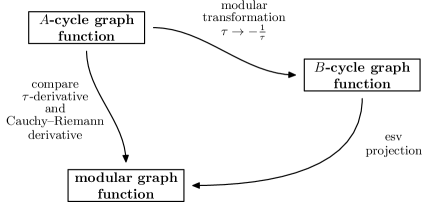
Figure 3: Two paths for the calculation of modular graph functions

The two different paths which can be taken in order to obtain modular graph functions from $A$-cycle graph functions are as follows:

• the first path starts from $A$-cycle graph functions and employs the similarity between the $\tau$-derivative on the $A$-cycle graph functions and the Cauchy–Riemann derivative acting on modular graph functions. Using the appropriate derivatives multiple times on both sides of the correspondence allows to successively infer the elements of the modular graph functions from their $A$-cycle graph analogues. This method is described in subsection 4.2.

• for the second path one converts $A$-cycle graph functions into $B$-cycle ones. Following this step, the projection esv is applied, which we conjecture to be an elliptic analogue of the single-valued projection sv mentioned in eq. (1.2). While the conversion from $A$- to $B$-cycle graph functions using a modular transformation has been described in subsection 3.3, the map esv will be described and discussed in subsection 4.3.

Both methods yield the same results, which are simultaneously in agreement with all expressions for modular graph functions calculated before [1, 2, 3].

4.1 Comparing relations among $A$-cycle graph functions with relations among modular graph functions

Given the common graphical representation of $A$-cycle graph functions and modular graph functions it is tempting to investigate, whether the known relations for modular graph functions reviewed in subsection 2.3.2 have an echo for $A$-cycle graph functions.

The simplest relation among modular graph functions, $\operatorname{\text{{\boldmath D}}}\mkern-4.2mu\Big{[}\includegraphics[width=14.22636pt,align=c]{sv-15.mps}\Big{]}-\operatorname{\text{{\boldmath D}}}\mkern-4.2mu\Big{[}\includegraphics[width=14.22636pt,align=c]{sv-16.mps}\Big{]}=\zeta_{3}$ at weight three, translates into

$$\operatorname{\text{{\boldmath A}}}\mkern-4.2mu\Big{[}\includegraphics[width=14.22636pt,align=c]{sv-15.mps}\Big{]}-\operatorname{\text{{\boldmath A}}}\mkern-4.2mu\Big{[}\includegraphics[width=14.22636pt,align=c]{sv-16.mps}\Big{]} =\frac{1}{2}\operatorname{\zeta}_{3}+6\operatorname{\zeta}_{2}\operatorname{\omega}_{A}(0,1,0,0)\,,$$ (4.1)

and the weight-four relation eq. (2.47) leads to

$$\operatorname{\text{{\boldmath A}}}\mkern-4.2mu\Big{[}\includegraphics[width=14.22636pt,align=c]{sv-17.mps}\Big{]}-24\operatorname{\text{{\boldmath A}}}\mkern-4.2mu\Big{[}\includegraphics[width=14.22636pt,align=c]{sv-18.mps}\Big{]}+18\operatorname{\text{{\boldmath A}}}\mkern-4.2mu\Big{[}\includegraphics[width=14.22636pt,align=c]{sv-19.mps}\Big{]}-3\operatorname{\text{{\boldmath A}}}\mkern-4.2mu\Big{[}\includegraphics[width=14.22636pt,align=c]{sv-14.mps}\Big{]}^{2} =144\operatorname{\zeta}_{2}\operatorname{\omega}_{A}(0,0,0,0,2)-24\operatorname{\zeta}_{2}\operatorname{\omega}_{A}(0,0,2)-\frac{31}{2}\zeta_{4}\,,$$ (4.2)

where the right-hand sides have been obtained by simply plugging in our results from subsection 3.2.

The right-hand sides of the corresponding equations for modular graph functions, eqs. (2.46) and (2.47) read $\zeta_{3}$ and $0$, respectively. This is rather suggestive: a relation between $A$-cycle graph functions might imply a valid relation between modular graph functions by formally replacing

$$\operatorname{\omega}_{A}(\underline{m})\,\zeta_{\underline{n}}\rightarrow\operatorname{\omega}_{A}(\underline{m})\,\zeta^{\rm sv}_{\underline{n}}\,,$$ (4.3)

where the single-valued projection of MZVs has been discussed in eqs. (1.2) and (1.3), and we remind the reader of the multi-index notation $\underline{n}=(n_{1},n_{2},\ldots,n_{r})$. The ad-hoc prescription eq. (4.3) has the desired effect of replacing $\frac{1}{2}\zeta_{3}$ with $\zeta_{3}$ on the right-hand side of eq. (4.1). Similarly, $\zeta_{4}$ is mapped to zero on the right-hand side of eq. (4.2), and all instances of $\zeta_{2}\operatorname{\omega}_{A}(\underline{m})$ are suppressed. For brevity of notation below, let $X$ be the rational vector space generated by products of classical and elliptic MZVs vanishing after applying eq. (4.3). That is

$$X:=\langle\operatorname{\zeta}_{2}\omega_{A}(\underline{m}),\operatorname{\zeta}_{4}\omega_{A}(\underline{m}),\ldots,(2\operatorname{\zeta}_{3,5}+5\operatorname{\zeta}_{3}\operatorname{\zeta}_{5})\omega_{A}(\underline{m}),\ldots\rangle_{\mathbb{Q}}\,.$$ (4.4)

In the equations below we will write “mod $X$”, which means that we are not writing terms from the space $X$. At weight five, the expressions in eqs. (3.23), (3.24) and appendix E for $A$-cycle graph functions lead to the relations

$$40\operatorname{\text{{\boldmath A}}}\mkern-4.2mu\Big{[}\includegraphics[width=14.22636pt,align=c]{sv-23.mps}\Big{]} =300\operatorname{\text{{\boldmath A}}}\mkern-4.2mu\Big{[}\includegraphics[width=14.22636pt,align=c]{sv-24.mps}\Big{]}+120\operatorname{\text{{\boldmath A}}}\mkern-4.2mu\Big{[}\includegraphics[width=14.22636pt,align=c]{sv-14.mps}\Big{]}\operatorname{\text{{\boldmath A}}}\mkern-4.2mu\Big{[}\includegraphics[width=14.22636pt,align=c]{sv-16.mps}\Big{]}-276\operatorname{\text{{\boldmath A}}}\mkern-4.2mu\Big{[}\includegraphics[width=14.22636pt,align=c]{sv-26.mps}\Big{]}+\frac{7}{2}\zeta_{5}\ \ \ {\rm mod}\ X$$ (4.5)

$$\operatorname{\text{{\boldmath A}}}\mkern-4.2mu\Big{[}\includegraphics[width=14.22636pt,align=c]{sv-21.mps}\Big{]} =60\operatorname{\text{{\boldmath A}}}\mkern-4.2mu\Big{[}\includegraphics[width=14.22636pt,align=c]{sv-24.mps}\Big{]}+10\operatorname{\text{{\boldmath A}}}\mkern-4.2mu\Big{[}\includegraphics[width=14.22636pt,align=c]{sv-14.mps}\Big{]}\operatorname{\text{{\boldmath A}}}\mkern-4.2mu\Big{[}\includegraphics[width=14.22636pt,align=c]{sv-15.mps}\Big{]}-48\operatorname{\text{{\boldmath A}}}\mkern-4.2mu\Big{[}\includegraphics[width=14.22636pt,align=c]{sv-26.mps}\Big{]}+8\zeta_{5}\ \ \ {\rm mod}\ X$$ (4.6)

$$10\operatorname{\text{{\boldmath A}}}\mkern-4.2mu\Big{[}\includegraphics[width=14.22636pt,align=c]{sv-22.mps}\Big{]} =20\operatorname{\text{{\boldmath A}}}\mkern-4.2mu\Big{[}\includegraphics[width=14.22636pt,align=c]{sv-24.mps}\Big{]}-4\operatorname{\text{{\boldmath A}}}\mkern-4.2mu\Big{[}\includegraphics[width=14.22636pt,align=c]{sv-26.mps}\Big{]}+\frac{3}{2}\zeta_{5}\ \ \ {\rm mod}\ X$$ (4.7)

$$30\operatorname{\text{{\boldmath A}}}\mkern-4.2mu\Big{[}\includegraphics[width=14.22636pt,align=c]{sv-27.mps}\Big{]} =12\operatorname{\text{{\boldmath A}}}\mkern-4.2mu\Big{[}\includegraphics[width=14.22636pt,align=c]{sv-26.mps}\Big{]}+\frac{\zeta_{5}}{2}\ \ \ {\rm mod}\ X\,,$$ (4.8)

which – upon employing eq. (4.3) – yield relations (2.48) to (2.51) among modular graph functions. The validity of the connection between $A$-cycle graph functions and modular graph functions described above has been also checked for relations between $A$-cycle graph functions of weight six, see appendix F – applying eq. (4.3) reproduces the relations eq. (F.1) among modular graph functions from open-string input.

Note that the prescription in eq. (4.3) is ill-defined as it does depend on the particular representations of eMZVs. In particular, there exist many relations among eMZVs and classical MZVs: For instance, the combination $2\operatorname{\omega}_{A}(0,2,2)+\operatorname{\omega}_{A}(0,0,4)=3\zeta_{4}$ should in principle be annihilated by applying eq. (4.3), but the definition in eq. (4.3) leaves both terms $\operatorname{\omega}_{A}(0,2,2)$ and $\operatorname{\omega}_{A}(0,0,4)$ inert. However, this does not affect the statement of the following conjecture: Given a polynomial $\mathcal{P}$ in $A$-cycle graph functions and MZVs such that

$${\cal P}(\text{{\boldmath A}}[\mathcal{G}],\zeta_{\underline{n}})=0\ {\rm mod}\ X\,,$$ (4.9)

with some graphs $\mathcal{G}$, one can replace $\text{{\boldmath A}}[\mathcal{G}]\rightarrow\text{{\boldmath D}}[\mathcal{G}]$ and $\zeta_{\underline{n}}\rightarrow\zeta^{\rm sv}_{\underline{n}}$ in that polynomial to obtain a relation between modular graph functions

$${\cal P}(\text{{\boldmath D}}[\mathcal{G}],\zeta^{\rm sv}_{\underline{n}})=0\,.$$ (4.10)

While this alone is a beautiful result, we would like to turn it into a formalism to actually compute modular graph functions. The next two subsections are dedicated to the description of the two possible methods outlined in figure 3.

We emphasize that eqs. (4.9) and (4.10) only apply to modular graph functions and $A$-cycle graph functions that are defined by integrating monomials in Green functions (involving any number of punctures). In superstring amplitudes involving five or more legs and all massless heterotic-string amplitudes, however, one may encounter more general integrals which will require extensions of the correspondence in eqs. (4.9) and (4.10) between open- and closed-string expressions. The same caveat applies to the rest of this section.

4.2 Modular graph functions from $A$-cycle graph functions

Given that relations among $A$-cycle graph functions can be mapped to those of modular graph functions, a natural follow-up question concerns a mapping between the respective functions of $\tau$ themselves: eMZVs on the open-string side and, as will be shown below, real parts of iterated Eisenstein integrals on the closed-string side. For this purpose, we compare first-order differential operators, namely $\partial_{\tau}:=\frac{\partial}{\partial\tau}$ acting on $A$-cycle graph functions and the Cauchy–Riemann derivative $\nabla$ defined in eq. (2.56) acting on modular graph functions.

4.2.1 $\boldsymbol{\tau}$-derivatives versus Cauchy–Riemann equations

From the representation of $A$-cycle graph functions in terms of eMZVs, their $\tau$-derivatives can be conveniently computed using eq. (C.3). For instance, the expressions eqs. (3.15) and (3.17) straightforwardly imply that

$$2\pi i\partial_{\tau}\operatorname{\text{{\boldmath A}}}\mkern-4.2mu\Big{[}\includegraphics[width=14.22636pt,align=c]{sv-14.mps}\Big{]} =-2\operatorname{\omega}_{A}(0,3)$$

$$(2\pi i\partial_{\tau})^{2}\operatorname{\text{{\boldmath A}}}\mkern-4.2mu\Big{[}\includegraphics[width=14.22636pt,align=c]{sv-14.mps}\Big{]} =6\operatorname{G}_{4}^{0}$$ (4.11)

as well as

$$2\pi i\partial_{\tau}\operatorname{\text{{\boldmath A}}}\mkern-4.2mu\Big{[}\includegraphics[width=14.22636pt,align=c]{sv-16.mps}\Big{]} =3\operatorname{\omega}_{A}(0,0,4)-6\zeta_{2}\operatorname{\omega}_{A}(0,0,2)-4\zeta_{4}$$

$$(2\pi i\partial_{\tau})^{2}\operatorname{\text{{\boldmath A}}}\mkern-4.2mu\Big{[}\includegraphics[width=14.22636pt,align=c]{sv-16.mps}\Big{]} =-12\operatorname{\omega}_{A}(0,5)+12\zeta_{2}\operatorname{\omega}_{A}(0,3)$$ (4.12)

$$(2\pi i\partial_{\tau})^{3}\operatorname{\text{{\boldmath A}}}\mkern-4.2mu\Big{[}\includegraphics[width=14.22636pt,align=c]{sv-16.mps}\Big{]} =60\operatorname{G}_{6}^{0}-36\zeta_{2}\operatorname{G}_{4}^{0}\,,$$

see eq. (2.20) for our conventions for $\operatorname{G}_{k}^{0}$. In the previous subsection, relations between $A$-cycle graph functions were found to only resemble those of modular graph functions after dropping terms from the space $X$ defined in eq. (4.4). Hence, we shall consider the simpler differential equations obeyed by a hatted version of $A$-cycle graph functions, in which the terms projected to zero by eq. (4.3) are omitted:

$$\hat{\text{{\boldmath A}}}[\mathcal{G}] =\text{{\boldmath A}}[\mathcal{G}]\ {\rm mod}\ X\,.$$ (4.13)

The simplest examples of $\hat{\text{{\boldmath A}}}[\mathcal{G}]$ can be expressed as:

$$\operatorname{\hat{\text{{\boldmath A}}}}\mkern-4.2mu\Big{[}\includegraphics[width=14.22636pt,align=c]{sv-14.mps}\Big{]} =\operatorname{\omega}_{A}(0,0,2)\,,\ \ \ \ \ \ \operatorname{\hat{\text{{\boldmath A}}}}\mkern-4.2mu\Big{[}\includegraphics[width=14.22636pt,align=c]{sv-16.mps}\Big{]}=-\operatorname{\omega}_{A}(0,0,0,3)+\frac{1}{6}\operatorname{\omega}_{A}(0,3)$$

$$\operatorname{\hat{\text{{\boldmath A}}}}\mkern-4.2mu\Big{[}\includegraphics[width=14.22636pt,align=c]{sv-19.mps}\Big{]} =\operatorname{\omega}_{A}(0,0,0,0,4)-\frac{1}{6}\operatorname{\omega}_{A}(0,0,4)$$ (4.14)

$$\operatorname{\hat{\text{{\boldmath A}}}}\mkern-4.2mu\Big{[}\includegraphics[width=14.22636pt,align=c]{sv-26.mps}\Big{]} =-\operatorname{\omega}_{A}(0,0,0,0,0,5)+\frac{1}{6}\operatorname{\omega}_{A}(0,0,0,5)-\frac{7}{360}\operatorname{\omega}_{A}(0,5)$$

$$\operatorname{\hat{\text{{\boldmath A}}}}\mkern-4.2mu\Big{[}\includegraphics[width=14.22636pt,align=c]{sv-18.mps}\Big{]} =\frac{1}{2}\operatorname{\omega}_{A}({0,0,2})^{2}-\frac{1}{2}\operatorname{\omega}_{A}({0,0,0,0,4})-\operatorname{\omega}_{A}({0,0,0,2,2})\,.$$

Writing the analogue of eq. (4.12) for $\hat{\text{{\boldmath A}}}[\mathcal{G}]$, the Eisenstein series $\operatorname{G}_{4}^{0}$ in the last line is no longer existent. Considering other simple graphs, one finds for instance

$$(2\pi i\partial_{\tau})^{2}\operatorname{\hat{\text{{\boldmath A}}}}\mkern-4.2mu\Big{[}\includegraphics[width=14.22636pt,align=c]{sv-14.mps}\Big{]} =6\operatorname{G}_{4}^{0}\,,\ \ \ \ \ \ \ (2\pi i\partial_{\tau})^{3}\operatorname{\hat{\text{{\boldmath A}}}}\mkern-4.2mu\Big{[}\includegraphics[width=14.22636pt,align=c]{sv-16.mps}\Big{]}=60\operatorname{G}_{6}^{0}$$ (4.15)

$$(2\pi i\partial_{\tau})^{4}\operatorname{\hat{\text{{\boldmath A}}}}\mkern-4.2mu\Big{[}\includegraphics[width=14.22636pt,align=c]{sv-19.mps}\Big{]} =840\operatorname{G}_{8}^{0}\,,\ \ \ \ (2\pi i\partial_{\tau})^{5}\operatorname{\hat{\text{{\boldmath A}}}}\mkern-4.2mu\Big{[}\includegraphics[width=14.22636pt,align=c]{sv-26.mps}\Big{]}=15120\operatorname{G}_{10}^{0}\,,$$

which intriguingly resemble the following instances of eq. (2.57):

$$(\pi\nabla)^{2}\operatorname{\text{{\boldmath D}}}\mkern-4.2mu\Big{[}\includegraphics[width=14.22636pt,align=c]{sv-14.mps}\Big{]} =6\,(\operatorname{Im}(\tau))^{4}\operatorname{G}_{4}\,,\ \ \ \ \ \ \ (\pi\nabla)^{3}\operatorname{\text{{\boldmath D}}}\mkern-4.2mu\Big{[}\includegraphics[width=14.22636pt,align=c]{sv-16.mps}\Big{]}=60\,(\operatorname{Im}(\tau))^{6}\operatorname{G}_{6}$$ (4.16)

$$(\pi\nabla)^{4}\operatorname{\text{{\boldmath D}}}\mkern-4.2mu\Big{[}\includegraphics[width=14.22636pt,align=c]{sv-19.mps}\Big{]} =840\,(\operatorname{Im}(\tau))^{8}\operatorname{G}_{8}\,,\ \ \ \ (\pi\nabla)^{5}\operatorname{\text{{\boldmath D}}}\mkern-4.2mu\Big{[}\includegraphics[width=14.22636pt,align=c]{sv-26.mps}\Big{]}=15120\,(\operatorname{Im}(\tau))^{10}\operatorname{G}_{10}\,.$$

A similar correspondence can be established for graphs with more than one loop: For instance, the expression for $\operatorname{\hat{\text{{\boldmath A}}}}\mkern-4.2mu\Big{[}\includegraphics[width=14.22636pt,align=c]{sv-18.mps}\Big{]}$ in eq. (4.14) yields

$$(2\pi i\partial_{\tau})^{3}\operatorname{\hat{\text{{\boldmath A}}}}\mkern-4.2mu\Big{[}\includegraphics[width=14.22636pt,align=c]{sv-18.mps}\Big{]} =12\operatorname{G}_{4}^{0}\operatorname{\omega}_{A}(0,3)-108\operatorname{\omega}_{A}(0,7)-72\zeta_{4}\operatorname{\omega}_{A}(0,3)$$ (4.17)

$$=-6\operatorname{G}_{4}^{0}2\pi i\partial_{\tau}\operatorname{\hat{\text{{\boldmath A}}}}\mkern-4.2mu\Big{[}\includegraphics[width=14.22636pt,align=c]{sv-14.mps}\Big{]}+\frac{9}{10}(2\pi i\partial_{\tau})^{3}\operatorname{\hat{\text{{\boldmath A}}}}\mkern-4.2mu\Big{[}\includegraphics[width=14.22636pt,align=c]{sv-19.mps}\Big{]}\ {\rm mod}\ X\,,$$

which resembles the differential equation (2.58) among modular graph functions

$$(\pi\nabla)^{3}\operatorname{\text{{\boldmath D}}}\mkern-4.2mu\Big{[}\includegraphics[width=14.22636pt,align=c]{sv-18.mps}\Big{]}=-6(\operatorname{Im}(\tau))^{4}\operatorname{G}_{4}\pi\nabla\operatorname{\text{{\boldmath D}}}\mkern-4.2mu\Big{[}\includegraphics[width=14.22636pt,align=c]{sv-14.mps}\Big{]}+\frac{9}{10}(\pi\nabla)^{3}\operatorname{\text{{\boldmath D}}}\mkern-4.2mu\Big{[}\includegraphics[width=14.22636pt,align=c]{sv-19.mps}\Big{]}\,.$$ (4.18)

In passing to the second line of eq. (4.17), we have identified $2\pi i\partial_{\tau}\operatorname{\hat{\text{{\boldmath A}}}}\mkern-4.2mu\Big{[}\includegraphics[width=14.22636pt,align=c]{sv-14.mps}\Big{]}=-2\operatorname{\omega}_{A}(0,3)$ as well as $(2\pi i\partial_{\tau})^{3}\operatorname{\hat{\text{{\boldmath A}}}}\mkern-4.2mu\Big{[}\includegraphics[width=14.22636pt,align=c]{sv-19.mps}\Big{]}=-120\operatorname{\omega}_{A}(0,7)$ and dropped $-72\zeta_{4}\operatorname{\omega}_{A}(0,3)$ as it is contained in the space $X$ defined in eq. (4.4). In a similar way, discarding terms from $X$ in the third $\tau$-derivative of $\operatorname{\text{{\boldmath A}}}\mkern-4.2mu\Big{[}\includegraphics[width=14.22636pt,align=c]{sv-24.mps}\Big{]}$ gives rise to an open-string counterpart of eq. (2.59).

We infer the following general conjecture from the above examples: Suppose that $A$-cycle graph functions associated with some graphs $\mathcal{G}$ satisfy the differential equation

$${\cal Q}(2\pi i\partial_{\tau},\operatorname{G}_{2k}^{0},\text{{\boldmath A}}[\mathcal{G}])=0\ {\rm mod}\ X\,,$$ (4.19)

with some polynomial ${\cal Q}$ in $\operatorname{G}_{2k}^{0}(2\pi i\partial_{\tau})^{n}\text{{\boldmath A}}[\mathcal{G}]$ where $k,n\geq 0$. Then, one can coherently replace $\text{{\boldmath A}}[\mathcal{G}]\rightarrow\text{{\boldmath D}}[\mathcal{G}]$ as well as $2\pi i\partial_{\tau}\rightarrow\pi\nabla$ and $\operatorname{G}_{2k}^{0}\rightarrow(\operatorname{Im}(\tau))^{2k}\operatorname{G}_{2k}$ in that polynomial and obtain a Cauchy–Riemann equation among modular graph functions

$${\cal Q}(\pi\nabla,(\operatorname{Im}(\tau))^{2k}\operatorname{G}_{2k},\text{{\boldmath D}}[\mathcal{G}])=0\,.$$ (4.20)

This procedure has been used at weight $w=5,6$ to derive conjectural Cauchy–Riemann differential equations for modular graph functions from $A$-cycle graph functions and thus constitutes an alternative way compared to the graphical manipulations of refs. [7, 11]. Our method has been checked to either reproduce the Cauchy–Riemann equations in the above reference or to yield expressions for modular graph functions that satisfy the Laplace equations in subsection 2.3.3 as discussed in the following section.

4.2.2 Integrating Cauchy–Riemann equations

We shall now describe techniques to convert Cauchy–Riemann equations derived via eqs. (4.19) and (4.20) into explicit representations of modular graph functions. The idea is to solve the differential equations in terms of iterated Eisenstein integrals eq. (2.19) along with integer powers of $\operatorname{Im}(\tau)$ and to fix the integration constants via modular invariance and reality of $\text{{\boldmath D}}[\mathcal{G}]$. However, these constraints do not fix the last integration constant which amounts to adding MZVs of the appropriate weight to the modular graph function under investigations. This shortcoming can be fixed either by numerical evaluation or by employing the alternative method described in subsection 4.3.

In case of one-loop graphs, eq. (2.57) can be integrated to yield the representation eq. (2.34) of non-holomorphic Eisenstein series $\operatorname{E}_{k}$ up to integration constants and antiholomorphic iterated Eisenstein integrals. The case $k=2$ in eq. (2.57) reads

$$(\pi\nabla)^{2}\operatorname{E}_{2}=6(\operatorname{Im}(\tau))^{4}\operatorname{G}_{4}$$ (4.21)

which – upon integration in $\tau$ – yields

$$\pi\nabla\operatorname{E}_{2}=\frac{2y^{3}}{45}+c_{1}\zeta_{3}+24y^{2}\operatorname{\mathcal{E}_{0}}(4)+12y\operatorname{\mathcal{E}_{0}}(4,0)+3\operatorname{\mathcal{E}_{0}}(4,0,0)+c_{2}\overline{\operatorname{\mathcal{E}_{0}}(4,0,0)}$$ (4.22)

with rational constants $c_{1},c_{2}$ and $y=\pi\operatorname{Im}(\tau)$. Then, a further integration gives rise to

$$\operatorname{E}_{2}=\frac{y^{2}}{45}-c_{1}\frac{\zeta_{3}}{y}-6\operatorname{\mathcal{E}_{0}}({4,0})+c_{3}\overline{\operatorname{\mathcal{E}_{0}}({4,0})}-\frac{3}{y}\operatorname{\mathcal{E}_{0}}({4,0,0})-\frac{c_{2}}{y}\overline{\operatorname{\mathcal{E}_{0}}({4,0,0})}$$ (4.23)

with another rational constant $c_{3}$. While performing the above integrations, we have used that Cauchy–Riemann derivatives act via

$$\pi\nabla(y^{n})=n\,y^{n+1}\,,\ \ \ \ \ \ \pi\nabla(\operatorname{\mathcal{E}_{0}}(k_{1},k_{2},\ldots,k_{r}))=\frac{4y^{2}}{(2\pi i)^{k_{r}}}\,\operatorname{G}_{k_{r}}^{0}\,\operatorname{\mathcal{E}_{0}}(k_{1},k_{2},\ldots,k_{r-1})\,,$$ (4.24)

and the integration constants $c_{i}\in\mathbb{Q}$ have been introduced following two selection rules:

• Let $\text{{\boldmath D}}[\mathcal{G}_{w}]$ denote a modular graph function of weight $w$, then the admissible integration constants in $(\pi\nabla)^{n}\text{{\boldmath D}}[\mathcal{G}_{w}]$ without any accompanying $\overline{\operatorname{\mathcal{E}_{0}}(\underline{k})}$ are rational combinations of single-valued MZVs of weight $w{+}n$.

• Whenever $(\pi\nabla)^{n}\text{{\boldmath D}}[\mathcal{G}_{w}]$ contains a term $\zeta^{\rm sv}_{\underline{m}}\operatorname{\mathcal{E}_{0}}(\underline{k})$, then rational multiples of its complex conjugate $\zeta^{\rm sv}_{\underline{m}}\overline{\operatorname{\mathcal{E}_{0}}(\underline{k})}$ have to be included in the integration constant.

Note that, as a consequence of (i), there is no rational multiple of $\zeta_{2}$ in eq. (4.23).

The rational constants $c_{i}\in\mathbb{Q}$ in eq. (4.23) can be fixed by imposing reality $\text{{\boldmath D}}[\mathcal{G}_{w}]=\overline{\text{{\boldmath D}}[\mathcal{G}_{w}]}$ and modular invariance: Reality requires the coefficients of $\operatorname{\mathcal{E}_{0}}({4,0})$ and $\overline{\operatorname{\mathcal{E}_{0}}({4,0})}$ as well as $\operatorname{\mathcal{E}_{0}}({4,0,0})$ and $\overline{\operatorname{\mathcal{E}_{0}}({4,0,0})}$ to match, yielding $c_{2}=3$ and $c_{3}=-6$. Then, the modular transformations eqs. (3.52) and (3.53) of $\operatorname{\mathcal{E}_{0}}({4,0}),\operatorname{\mathcal{E}_{0}}({4,0,0})$ and their complex conjugates introduce $\zeta_{3}$ in a way such that eq. (4.23) can only be modular invariant for $c_{1}=-1$. Hence, we arrive at

$$\operatorname{E}_{2}=\frac{y^{2}}{45}+\frac{\zeta_{3}}{y}-12\operatorname{Re}[\operatorname{\mathcal{E}_{0}}({4,0})]-\frac{6}{y}\operatorname{Re}[\operatorname{\mathcal{E}_{0}}({4,0,0})]\,,$$ (4.25)

which agrees with eq. (2.34). However, the criterion based on modular invariance still leaves the freedom to add single-valued MZVs to $\text{{\boldmath D}}[\mathcal{G}_{w}]$ which do not exist in the case at hand with $w=2$. When applying the above integration procedure to obtain the expressions

$$\operatorname{E}_{3} =\frac{2y^{3}}{945}+\frac{3\zeta_{5}}{4y^{2}}-120\operatorname{Re}[\operatorname{\mathcal{E}_{0}}({6,0,0})]-\frac{180}{y}\operatorname{Re}[\operatorname{\mathcal{E}_{0}}({6,0,0,0})]-\frac{90}{y^{2}}\operatorname{Re}[\operatorname{\mathcal{E}_{0}}({6,0,0,0,0})]$$ (4.26)

$$\operatorname{E}_{4} =\frac{y^{4}}{4725}+\frac{5\zeta_{7}}{8y^{3}}-1680\operatorname{Re}[\operatorname{\mathcal{E}_{0}}({8,0,0,0})]-\frac{5040}{y}\operatorname{Re}[\operatorname{\mathcal{E}_{0}}({8,0,0,0,0})]$$

$$\ \ \ \ \ -\frac{6300}{y^{2}}\operatorname{Re}[\operatorname{\mathcal{E}_{0}}({8,0,0,0,0,0})]-\frac{3150}{y^{3}}\operatorname{Re}[\operatorname{\mathcal{E}_{0}}({8,0,0,0,0,0,0})]$$ (4.27)

at weight $w=3,4$, the absence of $\zeta_{3}$ in $\operatorname{E}_{3}$ must be checked either by numerical evaluation or by the methods of section 4.3.

Note that the task of integrating Cauchy–Riemann equations is completely analogous to computing modular transformations of iterated Eisenstein integrals from their differential equations, see section 3.3.4. In particular, the differential operator $\sim\tau^{2}\partial_{\tau}$ for recursive computations of $B$-cycle graph functions in eqs. (3.49) to (3.51) can be mapped to the Cauchy–Riemann derivative eq. (2.56) by replacing $\tau^{2}\partial_{\tau}\rightarrow(\operatorname{Im}\tau)^{2}\partial_{\tau}$. This is another reason to expect strong parallels between $B$-cycle graph functions and modular graph functions.

4.2.3 Simplifying Cauchy–Riemann equations for multi-loop graphs

When applying the integration procedure of the previous subsection to modular graph functions corresponding to graphs with more than one loop, it is useful to disentangle iterated Eisenstein integrals with different types of entries. For instance, the simplest irreducible two-loop modular graph function $\operatorname{\text{{\boldmath D}}}\mkern-4.2mu\Big{[}\includegraphics[width=14.22636pt,align=c]{sv-18.mps}\Big{]}$ will comprise two kinds of iterated Eisenstein integrals involving either two instances of $\operatorname{G}_{4}^{0}$ or a single integration kernel $\operatorname{G}_{8}^{0}$. Any appearance of $\operatorname{G}_{8}^{0}$ in modular graph functions at weight four can be captured via $\operatorname{E}_{4}$, so it is convenient to study the linear combination

$$\operatorname{E}_{2,2}:=\operatorname{\text{{\boldmath D}}}\mkern-4.2mu\Big{[}\includegraphics[width=14.22636pt,align=c]{sv-18.mps}\Big{]}-\frac{9}{10}\operatorname{E}_{4}$$ (4.28)

for which the Cauchy–Riemann equation (4.18) simplifies to

$$(\pi\nabla)^{3}\operatorname{E}_{2,2}=-6\operatorname{Im}(\tau)^{4}\operatorname{G}_{4}\pi\nabla\operatorname{E}_{2}\,.$$ (4.29)

Then, starting from the representation (4.25) of $\operatorname{E}_{2}$, integration of eq. (4.29) yields depth-two iterated Eisenstein integrals with two entries of $\operatorname{G}_{4}^{0}$. This observation motivates us to define the depth of a modular graph function to be the minimum depth of the iterated Eisenstein integrals required to represent it, see section 2.2.2. Hence, the object $\operatorname{E}_{2,2}$ in eq. (4.28) is our simplest example of a modular graph function of depth two.

Similarly, Cauchy–Riemann equations at higher weight (which can be extracted from refs. [7, 11] and which we obtained from employing the correspondence in eqs. (4.19) and (4.20)) simplify when considering the following combinations:

$$\operatorname{E}_{2,3} =\operatorname{\text{{\boldmath D}}}\mkern-4.2mu\Big{[}\includegraphics[width=14.22636pt,align=c]{sv-24.mps}\Big{]}-\frac{43}{35}\text{E}_{5}$$ (4.30)

$$\operatorname{E}_{3,3} =3\operatorname{\text{{\boldmath D}}}\mkern-4.2mu\Big{[}\includegraphics[width=14.22636pt,align=c]{sv-41.mps}\Big{]}+\operatorname{\text{{\boldmath D}}}\mkern-4.2mu\Big{[}\includegraphics[width=14.22636pt,align=c]{sv-42.mps}\Big{]}-\frac{15}{14}\text{E}_{6}$$ (4.31)

$$\text{E}^{\prime}_{3,3} =\operatorname{\text{{\boldmath D}}}\mkern-4.2mu\Big{[}\includegraphics[width=14.22636pt,align=c]{sv-41.mps}\Big{]}+\frac{17}{60}\operatorname{\text{{\boldmath D}}}\mkern-4.2mu\Big{[}\includegraphics[width=14.22636pt,align=c]{sv-42.mps}\Big{]}-\frac{59}{140}\text{E}_{6}$$ (4.32)

$$\operatorname{E}_{2,4} =9\operatorname{\text{{\boldmath D}}}\mkern-4.2mu\Big{[}\includegraphics[width=14.22636pt,align=c]{sv-40.mps}\Big{]}+3\operatorname{\text{{\boldmath D}}}\mkern-4.2mu\Big{[}\includegraphics[width=14.22636pt,align=c]{sv-41.mps}\Big{]}+\operatorname{\text{{\boldmath D}}}\mkern-4.2mu\Big{[}\includegraphics[width=14.22636pt,align=c]{sv-42.mps}\Big{]}-13\text{E}_{6}$$ (4.33)

$$\operatorname{E}_{2,2,2} =-\operatorname{\text{{\boldmath D}}}\mkern-4.2mu\Big{[}\includegraphics[width=14.22636pt,align=c]{sv-43.mps}\Big{]}+\frac{232}{45}\operatorname{\text{{\boldmath D}}}\mkern-4.2mu\Big{[}\includegraphics[width=14.22636pt,align=c]{sv-42.mps}\Big{]}+\frac{292}{15}\operatorname{\text{{\boldmath D}}}\mkern-4.2mu\Big{[}\includegraphics[width=14.22636pt,align=c]{sv-41.mps}\Big{]}+\frac{2}{5}\operatorname{\text{{\boldmath D}}}\mkern-4.2mu\Big{[}\includegraphics[width=14.22636pt,align=c]{sv-40.mps}\Big{]}+2\text{E}_{3}^{2}+\text{E}_{2}\text{E}_{4}-\frac{466}{45}\text{E}_{6}\,.$$ (4.34)

The above combinations can be thought of as higher-depth generalizations of non-holomorphic Eisenstein series. The benefit of the subtractions of $\text{E}_{k}$ in eq. (4.30) to eq. (4.34) becomes apparent in

$$(\pi\nabla)^{3}\operatorname{E}_{2,3} =-2(\pi\nabla\text{E}_{2})(\pi\nabla)^{2}\text{E}_{3}-4\operatorname{Im}(\tau)^{4}\operatorname{G}_{4}\pi\nabla\text{E}_{3}$$ (4.35)

$$(\pi\nabla)^{5}\operatorname{E}_{3,3} =180\operatorname{Im}(\tau)^{6}\operatorname{G}_{6}(\pi\nabla)^{2}\text{E}_{3}$$ (4.36)

$$(\pi\nabla)^{4}\,\text{E}^{\prime}_{3,3} =-12\operatorname{Im}(\tau)^{6}\operatorname{G}_{6}(\pi\nabla)\text{E}_{3}$$ (4.37)

$$(\pi\nabla)^{3}\operatorname{E}_{2,4} =-27\operatorname{Im}(\tau)^{4}\operatorname{G}_{4}(\pi\nabla)\text{E}_{4}+\text{R}_{2,4}$$ (4.38)

$$\pi\nabla\,\text{R}_{2,4} =-81\operatorname{Im}(\tau)^{4}\operatorname{G}_{4}(\pi\nabla)^{2}\text{E}_{4}-27(\pi\nabla)\text{E}_{2}(\pi\nabla)^{3}\text{E}_{4}$$ (4.39)

from which we can anticipate all of $\operatorname{E}_{2,3},\operatorname{E}_{3,3},\text{E}^{\prime}_{3,3}$ and $\operatorname{E}_{2,4}$ to be of depth two. Finally, modular graph functions at weight six contain one independent depth-three representative satisfying

$$(\pi\nabla)^{3}\operatorname{E}_{2,2,2} =-12\operatorname{Im}(\tau)^{4}\operatorname{G}_{4}\pi\nabla\operatorname{E}_{2,2}+(\pi\nabla\text{E}_{2})^{3}\,.$$ (4.40)

For all terms $\nabla^{n}\text{E}_{\underline{k}}$ on the right-hand side of the above Cauchy–Riemann equations, a representation in terms of iterated Eisenstein integrals $\operatorname{\mathcal{E}_{0}}$ can be found in appendix G.1. We will now proceed to solving eq. (4.29) and eqs. (4.35) to (4.40) using the method in subsection 4.2.2.

4.2.4 Explicit solutions to Cauchy–Riemann equations at higher depth

For the simplest modular graph function of depth two, $\operatorname{E}_{2,2}$, the differential equation eq. (4.29) can be integrated to yield

$$\operatorname{E}_{2,2} =-\frac{y^{4}}{20250}+\frac{y\zeta_{3}}{45}+\frac{5\zeta_{5}}{12y}-\frac{\zeta_{3}^{2}}{4y^{2}}-\Big{(}\frac{2y}{15}-\frac{3\zeta_{3}}{y^{2}}\Big{)}\operatorname{Re}[\operatorname{\mathcal{E}_{0}}(4,0,0)]$$

$$-\frac{9}{2y^{2}}\big{(}\operatorname{Re}[\operatorname{\mathcal{E}_{0}}(4,0,0)]^{2}+\operatorname{Im}[\operatorname{\mathcal{E}_{0}}(4,0,0)]^{2}\big{)}-72\operatorname{Re}[\operatorname{\mathcal{E}_{0}}(4,4,0,0)]-\frac{1}{5}\operatorname{Re}[\operatorname{\mathcal{E}_{0}}(4,0,0,0)]$$

$$-\frac{36\operatorname{Re}[\operatorname{\mathcal{E}_{0}}(4,0,4,0,0)]}{y}-\frac{108\operatorname{Re}[\operatorname{\mathcal{E}_{0}}(4,4,0,0,0)]}{y}-\frac{\operatorname{Re}[\operatorname{\mathcal{E}_{0}}(4,0,0,0,0)]}{10y}$$ (4.41)

$$-\frac{9\operatorname{Re}[\operatorname{\mathcal{E}_{0}}(4,0,0,4,0,0)]}{y^{2}}-\frac{27\operatorname{Re}[\operatorname{\mathcal{E}_{0}}(4,0,4,0,0,0)]}{y^{2}}-\frac{54\operatorname{Re}[\operatorname{\mathcal{E}_{0}}(4,4,0,0,0,0)]}{y^{2}}\ ,$$

see eq. (G.1) for a convenient representation of the factor $\nabla\text{E}_{2}$ therein. Unlike the expression for $\operatorname{E}_{k}$, eq. (4.41) contains products of holomorphic and antiholomorphic iterated Eisenstein integrals, for example in

$$\operatorname{Re}[\operatorname{\mathcal{E}_{0}}(4,0,0)]^{2}=\frac{1}{4}\operatorname{\mathcal{E}_{0}}(4,0,0)^{2}+\frac{1}{2}\operatorname{\mathcal{E}_{0}}(4,0,0)\overline{\operatorname{\mathcal{E}_{0}}(4,0,0)}+\frac{1}{4}\overline{\operatorname{\mathcal{E}_{0}}(4,0,0)}^{2}$$ (4.42)

and $\operatorname{Im}[\operatorname{\mathcal{E}_{0}}(4,0,0)]^{2}$. The latter can be eliminated from eq. (4.41) by taking the real part of $\operatorname{\mathcal{E}_{0}}(4,0,0)^{2}$ and taking the shuffle relation

$$\operatorname{\mathcal{E}_{0}}(4,0,0)^{2}=2\operatorname{\mathcal{E}_{0}}(4,0,0,4,0,0)+6\operatorname{\mathcal{E}_{0}}(4,0,4,0,0,0)+12\operatorname{\mathcal{E}_{0}}(4,4,0,0,0,0)\ ,$$ (4.43)

into account. This manipulation turns out to cancel all iterated Eisenstein integrals of length six from eq. (4.41):

$$\operatorname{E}_{2,2} =-\frac{y^{4}}{20250}+\frac{y\zeta_{3}}{45}+\frac{5\zeta_{5}}{12y}-\frac{\zeta_{3}^{2}}{4y^{2}}-\Big{(}\frac{2y}{15}-\frac{3\zeta_{3}}{y^{2}}\Big{)}\operatorname{Re}[\operatorname{\mathcal{E}_{0}}(4,0,0)]$$

$$-\frac{9\operatorname{Re}[\operatorname{\mathcal{E}_{0}}(4,0,0)]^{2}}{y^{2}}-72\operatorname{Re}[\operatorname{\mathcal{E}_{0}}(4,4,0,0)]-\frac{1}{5}\operatorname{Re}[\operatorname{\mathcal{E}_{0}}(4,0,0,0)]$$ (4.44)

$$-\frac{36\operatorname{Re}[\operatorname{\mathcal{E}_{0}}(4,0,4,0,0)]}{y}-\frac{108\operatorname{Re}[\operatorname{\mathcal{E}_{0}}(4,4,0,0,0)]}{y}-\frac{\operatorname{Re}[\operatorname{\mathcal{E}_{0}}(4,0,0,0,0)]}{10y}\,.$$

The coefficients of $\frac{\zeta_{5}}{y}$ and $\frac{\zeta_{3}^{2}}{y^{2}}$ in eqs. (4.41) and (4.44) appear as integration constants in intermediate steps and can by fixed by imposing modular invariance of eq. (4.44). We have checked the resulting expression for $\operatorname{\text{{\boldmath D}}}\mkern-4.2mu\Big{[}\includegraphics[width=14.22636pt,align=c]{sv-18.mps}\Big{]}$ to satisfy the Laplace eigenvalue equation (2.53), and its coefficient of $q^{1}\overline{q}^{0}$ has been verified to agree with the results of ref. [3]. By inserting the $q$-expansion eq. (2.21) of iterated Eisenstein integrals, any term in the expansion eq. (2.37) of modular graph functions around the cusp is readily available from eq. (4.44) and similar expressions below.

Similarly, the Cauchy–Riemann equation (4.35) for the depth-two modular graph function eq. (4.30) at weight five can be integrated to yield

$$\operatorname{E}_{2,3} =-\frac{4y^{5}}{297675}+\frac{2y^{2}\zeta_{3}}{945}-\frac{\zeta_{5}}{180}-\frac{\zeta_{3}\zeta_{5}}{2y^{3}}+\frac{7\zeta_{7}}{16y^{2}}-\Big{(}\frac{4y^{2}}{315}-\frac{3\zeta_{5}}{y^{3}}\Big{)}\operatorname{Re}[\operatorname{\mathcal{E}_{0}}(4,0,0)]$$

$$-\Big{(}\frac{8y}{3}-\frac{60\zeta_{3}}{y^{2}}\Big{)}\operatorname{Re}[\operatorname{\mathcal{E}_{0}}(6,0,0,0)]-\Big{(}8-\frac{60\zeta_{3}}{y^{3}}\Big{)}\operatorname{Re}[\operatorname{\mathcal{E}_{0}}(6,0,0,0,0)]$$

$$-\frac{360\operatorname{Re}[\operatorname{\mathcal{E}_{0}}(4,0,0)]\operatorname{Re}[\operatorname{\mathcal{E}_{0}}(6,0,0,0)]}{y^{2}}-\frac{360\operatorname{Re}[\operatorname{\mathcal{E}_{0}}(4,0,0)]\operatorname{Re}[\operatorname{\mathcal{E}_{0}}(6,0,0,0,0)]}{y^{3}}$$

$$-1440\operatorname{Re}[\operatorname{\mathcal{E}_{0}}(4,6,0,0,0)]+\frac{\operatorname{Re}[\operatorname{\mathcal{E}_{0}}(4,0,0,0,0)]}{21}-480\operatorname{Re}[\operatorname{\mathcal{E}_{0}}(6,0,4,0,0)]-1440\operatorname{Re}[\operatorname{\mathcal{E}_{0}}(6,4,0,0,0)]$$

$$-\frac{720\operatorname{Re}[\operatorname{\mathcal{E}_{0}}(4,0,6,0,0,0)]}{y}-\frac{4320\operatorname{Re}[\operatorname{\mathcal{E}_{0}}(4,6,0,0,0,0)]}{y}+\frac{\operatorname{Re}[\operatorname{\mathcal{E}_{0}}(4,0,0,0,0,0)]}{14y}$$ (4.45)

$$-\frac{720\operatorname{Re}[\operatorname{\mathcal{E}_{0}}(6,0,0,4,0,0)]}{y}-\frac{2160\operatorname{Re}[\operatorname{\mathcal{E}_{0}}(6,0,4,0,0,0)]}{y}-\frac{4320\operatorname{Re}[\operatorname{\mathcal{E}_{0}}(6,4,0,0,0,0)]}{y}$$

$$-\frac{10\operatorname{Re}[\operatorname{\mathcal{E}_{0}}(6,0,0,0,0,0)]}{y}-\frac{720\operatorname{Re}[\operatorname{\mathcal{E}_{0}}(4,0,6,0,0,0,0)]}{y^{2}}-\frac{3600\operatorname{Re}[\operatorname{\mathcal{E}_{0}}(4,6,0,0,0,0,0)]}{y^{2}}$$

$$+\frac{\operatorname{Re}[\operatorname{\mathcal{E}_{0}}(4,0,0,0,0,0,0)]}{28y^{2}}-\frac{360\operatorname{Re}[\operatorname{\mathcal{E}_{0}}(6,0,0,0,4,0,0)]}{y^{2}}-\frac{1080\operatorname{Re}[\operatorname{\mathcal{E}_{0}}(6,0,0,4,0,0,0)]}{y^{2}}$$

$$-\frac{2160\operatorname{Re}[\operatorname{\mathcal{E}_{0}}(6,0,4,0,0,0,0)]}{y^{2}}-\frac{3600\operatorname{Re}[\operatorname{\mathcal{E}_{0}}(6,4,0,0,0,0,0)]}{y^{2}}-\frac{5\operatorname{Re}[\operatorname{\mathcal{E}_{0}}(6,0,0,0,0,0,0)]}{y^{2}}\,,$$

see eqs. (G.2) and (G.3) for explicit expressions of $\nabla\text{E}_{3}$ and $\nabla^{2}\text{E}_{3}$. Following the strategy of simplifying $\text{E}_{2,2}$, we have eliminated the appearance of $\operatorname{Im}[\operatorname{\mathcal{E}_{0}}(4,0,0)]\operatorname{Im}[\operatorname{\mathcal{E}_{0}}(6,0,0,0)]$ and $\operatorname{Im}[\operatorname{\mathcal{E}_{0}}(4,0,0)]\operatorname{Im}[\operatorname{\mathcal{E}_{0}}(6,0,0,0,0)]$ in intermediate steps by taking the real part of appropriate shuffle relations. These manipulations also remove all iterated Eisenstein integrals of length $8$ from our final expression eq. (4.45). Hence, elimination of any $\operatorname{Im}[\operatorname{\mathcal{E}_{0}}(\ldots)]$ via shuffle relations will be our guiding principle for all subsequent cases which turns out to reduce the maximum length of the iterated Eisenstein integrals appearing in a given $\text{E}_{\underline{k}}$.

The coefficient of $\zeta_{5}$ in $\text{E}_{2,3}$ is not fixed by modular invariance and can be inferred by comparison with the results in the literature, numerical evaluation or by the method discussed in subsection 4.3. The expression for $\operatorname{\text{{\boldmath D}}}\mkern-4.2mu\Big{[}\includegraphics[width=14.22636pt,align=c]{sv-24.mps}\Big{]}$ resulting from eq. (4.45) has been checked to satisfy the Laplace equation (2.54), and its coefficient of $q^{1}\overline{q}^{0}$ agrees with the results of [3].

There are three independent modular graph functions at weight six and depth two: $\operatorname{E}_{3,3},\operatorname{E}_{3,3}^{\prime}$ as well as $\operatorname{E}_{2,4}$ defined in eqs. (4.31) to (4.33) are a convenient choice of basis. Integrating the Cauchy–Riemann equation (4.36) for $\operatorname{E}_{3,3}$ gives rise to

$$\operatorname{E}_{3,3} =\frac{2y^{6}}{6251175}+\frac{y\zeta_{5}}{210}+\frac{\zeta_{7}}{16y}-\frac{7\zeta_{9}}{64y^{3}}+\frac{9\zeta_{5}^{2}}{64y^{4}}-\Big{(}\frac{4y}{7}+\frac{135\zeta_{5}}{4y^{4}}\Big{)}\operatorname{Re}[\operatorname{\mathcal{E}_{0}}(6,0,0,0,0)]$$

$$+\frac{2025\operatorname{Re}[\operatorname{\mathcal{E}_{0}}(6,0,0,0,0)]^{2}}{y^{4}}+21600\operatorname{Re}[\operatorname{\mathcal{E}_{0}}(6,6,0,0,0,0)]-\frac{20}{7}\operatorname{Re}[\operatorname{\mathcal{E}_{0}}(6,0,0,0,0,0)]$$

$$+\frac{21600\operatorname{Re}[\operatorname{\mathcal{E}_{0}}(6,0,6,0,0,0,0)]}{y}+\frac{108000\operatorname{Re}[\operatorname{\mathcal{E}_{0}}(6,6,0,0,0,0,0)]}{y}$$

$$-\frac{45\operatorname{Re}[\operatorname{\mathcal{E}_{0}}(6,0,0,0,0,0,0)]}{7y}+\frac{16200\operatorname{Re}[\operatorname{\mathcal{E}_{0}}(6,0,0,6,0,0,0,0)]}{y^{2}}$$ (4.46)

$$+\frac{81000\operatorname{Re}[\operatorname{\mathcal{E}_{0}}(6,0,6,0,0,0,0,0)]}{y^{2}}+\frac{243000\operatorname{Re}[\operatorname{\mathcal{E}_{0}}(6,6,0,0,0,0,0,0)]}{y^{2}}$$

$$-\frac{15\operatorname{Re}[\operatorname{\mathcal{E}_{0}}(6,0,0,0,0,0,0,0)]}{2y^{2}}+\frac{8100\operatorname{Re}[\operatorname{\mathcal{E}_{0}}(6,0,0,0,6,0,0,0,0)]}{y^{3}}$$

$$+\frac{40500\operatorname{Re}[\operatorname{\mathcal{E}_{0}}(6,0,0,6,0,0,0,0,0)]}{y^{3}}+\frac{121500\operatorname{Re}[\operatorname{\mathcal{E}_{0}}(6,0,6,0,0,0,0,0,0)]}{y^{3}}$$

$$+\frac{283500\operatorname{Re}[\operatorname{\mathcal{E}_{0}}(6,6,0,0,0,0,0,0,0)]}{y^{3}}-\frac{15\operatorname{Re}[\operatorname{\mathcal{E}_{0}}(6,0,0,0,0,0,0,0,0)]}{4y^{3}}\,,$$

and similar expressions for $\text{E}^{\prime}_{3,3}$ and $\operatorname{E}_{2,4}$ based on eqs. (4.37) to (4.39) are provided in appendix G.2. The resulting expressions for $\operatorname{\text{{\boldmath D}}}\mkern-4.2mu\Big{[}\includegraphics[width=14.22636pt,align=c]{sv-40.mps}\Big{]},\operatorname{\text{{\boldmath D}}}\mkern-4.2mu\Big{[}\includegraphics[width=14.22636pt,align=c]{sv-41.mps}\Big{]}$ and $\operatorname{\text{{\boldmath D}}}\mkern-4.2mu\Big{[}\includegraphics[width=14.22636pt,align=c]{sv-42.mps}\Big{]}$ have been checked to satisfy the Laplace eigenvalue equations (2.55).

Finally, there is a single irreducible modular graph function of depth three at weight six: $\operatorname{E}_{2,2,2}$ defined in eq. (4.34). Integrating its Cauchy–Riemann equation (4.40) (with $\nabla\operatorname{E}_{2,2}$ spelt out in eq. (G.7)) yields

$$\operatorname{E}_{2,2,2} =\frac{4y^{6}}{9568125}-\frac{2y^{3}\zeta_{3}}{10125}+\frac{y\zeta_{5}}{54}+\frac{\zeta_{3}^{2}}{90}+\frac{661\zeta_{7}}{1800y}-\frac{5\zeta_{3}\zeta_{5}}{12y^{2}}+\frac{\zeta_{3}^{3}}{6y^{3}}$$

$$\!\!\!+\Big{(}\frac{4y^{3}}{3375}{-}\frac{2\zeta_{3}}{15}{+}\frac{5\zeta_{5}}{2y^{2}}{-}\frac{3\zeta_{3}^{2}}{y^{3}}\Big{)}\operatorname{Re}[\operatorname{\mathcal{E}_{0}}(4,0,0)]+\Big{(}\frac{2}{5}{+}\frac{18\zeta_{3}}{y^{3}}\Big{)}\operatorname{Re}[\operatorname{\mathcal{E}_{0}}(4,0,0)]^{2}-\frac{36\operatorname{Re}[\operatorname{\mathcal{E}_{0}}(4,0,0)]^{3}}{y^{3}}$$

$$\!\!\!-36\Big{(}\frac{2y}{45}-\frac{\zeta_{3}}{y^{2}}+\frac{6\operatorname{Re}[\operatorname{\mathcal{E}_{0}}(4,0,0)]}{y^{2}}\Big{)}\operatorname{Re}\!\Big{[}\operatorname{\mathcal{E}_{0}}(4,0,4,0,0)]+3\operatorname{\mathcal{E}_{0}}(4,4,0,0,0)+\frac{\operatorname{\mathcal{E}_{0}}(4,0,0,0,0)}{360}\Big{]}$$

$$\!\!\!-864\operatorname{Re}[\operatorname{\mathcal{E}_{0}}(4,4,0,4,0,0)]-2592\operatorname{Re}[\operatorname{\mathcal{E}_{0}}(4,4,4,0,0,0)]-\frac{12}{5}\operatorname{Re}[\operatorname{\mathcal{E}_{0}}(4,0,0,4,0,0)]$$

$$\!\!\!-\frac{36}{5}\operatorname{Re}[\operatorname{\mathcal{E}_{0}}(4,0,4,0,0,0)]-\frac{84}{5}\operatorname{Re}[\operatorname{\mathcal{E}_{0}}(4,4,0,0,0,0)]-\frac{1}{150}\operatorname{Re}[\operatorname{\mathcal{E}_{0}}(4,0,0,0,0,0)]$$ (4.47)

$$\!\!\!-\frac{1296\operatorname{Re}[\operatorname{\mathcal{E}_{0}}(4,4,0,0,4,0,0)]}{y}-\frac{3888\operatorname{Re}[\operatorname{\mathcal{E}_{0}}(4,4,0,4,0,0,0)]}{y}-\frac{7776\operatorname{Re}[\operatorname{\mathcal{E}_{0}}(4,4,4,0,0,0,0)]}{y}$$

$$\!\!\!-\frac{432\operatorname{Re}[\operatorname{\mathcal{E}_{0}}(4,0,4,0,4,0,0)]}{y}-\frac{1296\operatorname{Re}[\operatorname{\mathcal{E}_{0}}(4,0,4,4,0,0,0)]}{y}-\frac{6\operatorname{Re}[\operatorname{\mathcal{E}_{0}}(4,0,0,0,4,0,0)]}{5y}$$

$$\!\!\!-\frac{18\operatorname{Re}[\operatorname{\mathcal{E}_{0}}(4,0,0,4,0,0,0)]}{5y}-\frac{42\operatorname{Re}[\operatorname{\mathcal{E}_{0}}(4,0,4,0,0,0,0)]}{5y}$$

$$\!\!\!-\frac{18\operatorname{Re}[\operatorname{\mathcal{E}_{0}}(4,4,0,0,0,0,0)]}{y}-\frac{\operatorname{Re}[\operatorname{\mathcal{E}_{0}}(4,0,0,0,0,0,0)]}{300y}\,,$$

which, together with $\operatorname{E}_{3,3},\text{E}^{\prime}_{3,3}$ and $\operatorname{E}_{2,4}$, completes the basis of weight-six modular graph functions under the relations in appendix F. For all the above expressions for modular graph functions, modular invariance has been confirmed numerically.

All the above examples confirm our conjecture that the number of loops in a graph is an upper bound for the depth of the associated modular graph function. Said upper bound is saturated for the independent modular graph functions $\operatorname{\text{{\boldmath D}}}\mkern-4.2mu\Big{[}\includegraphics[width=14.22636pt,align=c]{sv-18.mps}\Big{]},\operatorname{\text{{\boldmath D}}}\mkern-4.2mu\Big{[}\includegraphics[width=14.22636pt,align=c]{sv-24.mps}\Big{]},\operatorname{\text{{\boldmath D}}}\mkern-4.2mu\Big{[}\includegraphics[width=14.22636pt,align=c]{sv-41.mps}\Big{]},\operatorname{\text{{\boldmath D}}}\mkern-4.2mu\Big{[}\includegraphics[width=14.22636pt,align=c]{sv-42.mps}\Big{]},\operatorname{\text{{\boldmath D}}}\mkern-4.2mu\Big{[}\includegraphics[width=14.22636pt,align=c]{sv-40.mps}\Big{]}$ and $\operatorname{\text{{\boldmath D}}}\mkern-4.2mu\Big{[}\includegraphics[width=14.22636pt,align=c]{sv-43.mps}\Big{]}$ at weight $w\leq 6$. However, $\operatorname{\text{{\boldmath D}}}\mkern-4.2mu\Big{[}\includegraphics[width=14.22636pt,align=c]{sv-15.mps}\Big{]}$ being of depth one (cf. eq. (2.46)) and $\operatorname{\text{{\boldmath D}}}\mkern-4.2mu\Big{[}\includegraphics[width=14.22636pt,align=c]{sv-28.mps}\Big{]}$ being of depth three (cf. eq. (F.1)) are examples where the loop order exceeds the depth.

4.2.5 Laplace equation at weight six

From their representations in terms of iterated Eisenstein integrals, we infer the following Laplace equation among modular graph functions which has not yet been spelt out in the literature:

$$(\Delta-2)\big{(}\operatorname{\text{{\boldmath D}}}\mkern-4.2mu\Big{[}\includegraphics[width=14.22636pt,align=c]{sv-43.mps}\Big{]}-2\operatorname{E}_{3}^{2}-\operatorname{E}_{2}\operatorname{E}_{4}\big{)}-\frac{14}{9}\operatorname{\text{{\boldmath D}}}\mkern-4.2mu\Big{[}\includegraphics[width=14.22636pt,align=c]{sv-42.mps}\Big{]}+\frac{16}{3}\operatorname{\text{{\boldmath D}}}\mkern-4.2mu\Big{[}\includegraphics[width=14.22636pt,align=c]{sv-41.mps}\Big{]}-4\operatorname{\text{{\boldmath D}}}\mkern-4.2mu\Big{[}\includegraphics[width=14.22636pt,align=c]{sv-40.mps}\Big{]}$$

$$\ \ \ \ \ +\frac{284}{9}\operatorname{E}_{6}+\frac{2}{3}\operatorname{E}_{2}^{3}+16\operatorname{E}_{3}^{2}+\frac{12}{5}\operatorname{E}_{2}\operatorname{E}_{4}-4\operatorname{E}_{2}\operatorname{E}_{2,2}=0\,.$$ (4.48)

The combination $\operatorname{\text{{\boldmath D}}}\mkern-4.2mu\Big{[}\includegraphics[width=14.22636pt,align=c]{sv-43.mps}\Big{]}-2\operatorname{E}_{3}^{2}-\operatorname{E}_{2}\operatorname{E}_{4}$ along with the Laplacian is designed to absorb contributions $\sim\partial_{\tau}\operatorname{E}_{p}\overline{\partial_{\tau}\operatorname{E}_{q}}$ in eq. (4.48) with $p+q=6$. Moreover, the combination $\operatorname{\text{{\boldmath D}}}\mkern-4.2mu\Big{[}\includegraphics[width=14.22636pt,align=c]{sv-43.mps}\Big{]}-2\operatorname{E}_{3}^{2}-\operatorname{E}_{2}\operatorname{E}_{4}$ is selected by the formalism of ref. [11] to linearize the relations between modular graph functions, as can be verified from the second equation from below in eq. (F.1).

4.2.6 Representations of modular graph functions in terms of $\operatorname{\mathcal{E}}$ rather than $\operatorname{\mathcal{E}_{0}}$?

While all expressions for modular graph functions or their constituents have been expressed in terms of iterated Eisenstein integrals $\operatorname{\mathcal{E}_{0}}$ defined in eq. (2.19), we conclude this subsection with expressions for modular graph functions in terms of iterated Eisenstein integrals $\operatorname{\mathcal{E}}$ defined in eq. (2.18), where the constant terms $2\zeta_{k}$ of the integrands $\operatorname{G}_{k}$ are not subtracted. At depth one, these $\operatorname{\mathcal{E}}$ appear to be the more suitable language for modular graph functions than the $\operatorname{\mathcal{E}_{0}}$ since the polynomial term $\operatorname{E}_{k}\sim y^{k}$ in eq. (2.35) is absorbed in this way:

$$\operatorname{E}_{k} =\frac{4\,(2k{-}3)!\,\zeta_{2k-1}\,(4y)^{1-k}}{(k{-}2)!\,(k{-}1)!}-8y(2k{-}1)!\sum\limits_{j=0}^{k-1}\binom{2k{-}2{-}j}{k{-}1}\frac{(4y)^{j-k}}{j!}\,\operatorname{Re}[\operatorname{\mathcal{E}}(2k,\underbrace{0,\ldots,0}_{2k-2-j};q)]\,.$$ (4.49)

However, the analogous rearrangements at depth two convert eq. (4.44) into

$$\operatorname{E}_{2,2} =\frac{\zeta_{3}\,|T|^{2}}{60y}+\frac{5\zeta_{5}}{12y}-\frac{\zeta_{3}^{2}}{4y^{2}}+\frac{3\zeta_{3}}{y^{2}}\operatorname{Re}[\operatorname{\mathcal{E}}(4,0,0)]-\frac{9\operatorname{Re}[\operatorname{\mathcal{E}}(4,0,0)]^{2}}{y^{2}}$$ (4.50)

$$-72\operatorname{Re}[\operatorname{\mathcal{E}}(4,4,0,0)]-\frac{36\operatorname{Re}[\operatorname{\mathcal{E}}(4,0,4,0,0)]}{y}-\frac{108\operatorname{Re}[\operatorname{\mathcal{E}}(4,4,0,0,0)]}{y}$$

and introduce an explicit appearance of $\operatorname{Re}\tau$ via $|T|^{2}=\pi^{2}((\operatorname{Re}\tau)^{2}+(\operatorname{Im}\tau)^{2})$. Similar observations have been made for $\operatorname{E}_{2,3}$ and examples at higher weight, so it is not clear if representations in terms of $\operatorname{\mathcal{E}}$ are preferable at generic depth.

4.3 Modular graph functions from $B$-cycle graph functions

In this section, we suggest a mapping between $B$-cycle graph functions and the corresponding modular graph functions which is based on their representations via iterated Eisenstein integrals (see subsection 3.3.5 and subsection 4.2.4, respectively).

4.3.1 Depth one

For illustrative purposes, we repeat the expressions

$$\operatorname{\text{{\boldmath D}}}\mkern-4.2mu\Big{[}\includegraphics[width=14.22636pt,align=c]{sv-14.mps}\Big{]} =\frac{y^{2}}{45}+\frac{\zeta_{3}}{y}-12\operatorname{Re}[\operatorname{\mathcal{E}_{0}}({4,0})]-\frac{6}{y}\operatorname{Re}[\operatorname{\mathcal{E}_{0}}({4,0,0})]$$

$$\operatorname{\text{{\boldmath D}}}\mkern-4.2mu\Big{[}\includegraphics[width=14.22636pt,align=c]{sv-16.mps}\Big{]} =\frac{2y^{3}}{945}+\frac{3\zeta_{5}}{4y^{2}}-120\operatorname{Re}[\operatorname{\mathcal{E}_{0}}({6,0,0})]-\frac{180}{y}\operatorname{Re}[\operatorname{\mathcal{E}_{0}}({6,0,0,0})]-\frac{90}{y^{2}}\operatorname{Re}[\operatorname{\mathcal{E}_{0}}({6,0,0,0,0})]$$

$$\operatorname{\text{{\boldmath D}}}\mkern-4.2mu\Big{[}\includegraphics[width=14.22636pt,align=c]{sv-19.mps}\Big{]} =\frac{y^{4}}{4725}+\frac{5\zeta_{7}}{8y^{3}}-1680\operatorname{Re}[\operatorname{\mathcal{E}_{0}}({8,0,0,0})]-\frac{5040}{y}\operatorname{Re}[\operatorname{\mathcal{E}_{0}}({8,0,0,0,0})]$$ (4.51)

$$\ \ \ \ \ -\frac{6300}{y^{2}}\operatorname{Re}[\operatorname{\mathcal{E}_{0}}({8,0,0,0,0,0})]-\frac{3150}{y^{3}}\operatorname{Re}[\operatorname{\mathcal{E}_{0}}({8,0,0,0,0,0,0})]\,,$$

for the simplest modular graph functions which agree with the all-weight formula eq. (2.34) for non-holomorphic Eisenstein series. These closed-string expressions will be brought into correspondence with the analogous $B$-cycle graph functions eq. (3.54) modulo $\zeta_{2}$ on the open-string side,

$$\operatorname{\text{{\boldmath B}}}\mkern-4.2mu\Big{[}\includegraphics[width=14.22636pt,align=c]{sv-14.mps}\Big{]} =\frac{T^{2}}{180}-\frac{\zeta_{3}}{T}-6\operatorname{\mathcal{E}_{0}}(4,0)+\frac{6\operatorname{\mathcal{E}_{0}}(4,0,0)}{T}\ {\rm mod}\ \zeta_{2}$$

$$\operatorname{\text{{\boldmath B}}}\mkern-4.2mu\Big{[}\includegraphics[width=14.22636pt,align=c]{sv-16.mps}\Big{]} =-\frac{T^{3}}{3780}+\frac{3\zeta_{5}}{2T^{2}}-60\operatorname{\mathcal{E}_{0}}(6,0,0)+\frac{180\operatorname{\mathcal{E}_{0}}(6,0,0,0)}{T}-\frac{180\operatorname{\mathcal{E}_{0}}(6,0,0,0,0)}{T^{2}}\ {\rm mod}\ \zeta_{2}$$

$$\operatorname{\text{{\boldmath B}}}\mkern-4.2mu\Big{[}\includegraphics[width=14.22636pt,align=c]{sv-19.mps}\Big{]} =\frac{T^{4}}{75600}-\frac{5\zeta_{7}}{2T^{3}}-840\operatorname{\mathcal{E}_{0}}(8,0,0,0)+\frac{5040\operatorname{\mathcal{E}_{0}}(8,0,0,0,0)}{T}$$ (4.52)

$$\ \ \ \ -\frac{12600\operatorname{\mathcal{E}_{0}}(8,0,0,0,0,0)}{T^{2}}+\frac{12600\operatorname{\mathcal{E}_{0}}(8,0,0,0,0,0,0)}{T^{3}}\ {\rm mod}\ \zeta_{2}\,.$$

As in eq. (3.57), the notion of “mod $\zeta_{2}$” refers to a representation of all the $\tau$-dependence via $T$ and $\operatorname{\mathcal{E}_{0}}(\underline{k})$, where all terms of the form $\zeta_{2}^{n}T^{m}\operatorname{\mathcal{E}_{0}}(\underline{k})$ with $n\geq 1$ and $m\in\mathbb{Z}$ are suppressed.

In comparing the above expressions for modular graph functions and $B$-cycle graph functions, both iterated Eisenstein integrals and Laurent polynomials in $y$ or $T$ exhibit striking similarities in their coefficients: every single term in eq. (4.52) will find a correspondent in eq. (4.51) once we replace

$$T\rightarrow-2y\,,\ \ \ \ \operatorname{\mathcal{E}_{0}}(2k,0,\ldots)\rightarrow 2\operatorname{Re}[\operatorname{\mathcal{E}_{0}}(2k,0,\ldots)]\,,\ \ \ \ \zeta_{2k+1}\rightarrow 2\zeta_{2k+1}\,,\ \ \ \ \zeta_{2k}\rightarrow 0\,.$$ (4.53)

The $\tau$ dependence of the $\operatorname{\mathcal{E}_{0}}(\underline{k})$ through their $q$-series eq. (2.21) is understood to be unaffected by the prescription $T\rightarrow-2y$. The same correspondence has been verified between the depth-one modular graph functions $\operatorname{\text{{\boldmath D}}}\mkern-4.2mu\Big{[}\includegraphics[width=14.22636pt,align=c]{sv-26.mps}\Big{]}$, $\operatorname{\text{{\boldmath D}}}\mkern-4.2mu\Big{[}\includegraphics[width=14.22636pt,align=c]{sv-39.mps}\Big{]}$ and their $B$-cycle counterparts $\operatorname{\text{{\boldmath B}}}\mkern-4.2mu\Big{[}\includegraphics[width=14.22636pt,align=c]{sv-26.mps}\Big{]}$, $\operatorname{\text{{\boldmath B}}}\mkern-4.2mu\Big{[}\includegraphics[width=14.22636pt,align=c]{sv-39.mps}\Big{]}$, where the latter has been inferred from the $A$-cycle counterpart of the relations in appendix F.

4.3.2 General form

Both the doubling of odd zeta-values in eq. (4.53) and the suppression of $\zeta_{2}$ in matching $B$-cycle graph functions with non-holomorphic Eisenstein series are reminiscent of the single-valued projection of MZVs. From the above examples associated with one-loop graphs, it is tempting to study the following generalization of eq. (4.53)

$${\rm esv}:\ \ \ \left\{\begin{aligned} (i)&\hskip 8.0pt&T&\rightarrow&&-2y\\ (ii)&&\operatorname{\mathcal{E}_{0}}(k_{1},k_{2},\ldots,k_{r})&\rightarrow&&2\operatorname{Re}[\operatorname{\mathcal{E}_{0}}(k_{1},k_{2},\ldots,k_{r})],\quad k_{1}\neq 0\\ (iii)&&\zeta_{\underline{n}}&\rightarrow&&\zeta^{\rm sv}_{\underline{n}}\end{aligned}\right.$$ (4.54)

to arbitrary MZVs and iterated Eisenstein integrals. Note that part $(i)$ is in fact a special case of Brown’s single valued map for multiple polylogarithms [79], because $2T=\log q$ is sent to $-4y=\log q+\log\overline{q}$. As before, part $(i)$ is understood to not act on the $q$-series eq. (2.21) of $\operatorname{\mathcal{E}_{0}}(k,\ldots)$ with $k\neq 0$. Moreover, part $(iii)$ motivates our earlier choices to occasionally display $B$-cycle graph function modulo terms sent to zero by the esv-map such as $\zeta_{2}T^{m}\operatorname{\mathcal{E}_{0}}(\underline{k})$. As the key result of this section, we conjecture that, once a $B$-cycle graph function is suitably expressed in terms of $T$ and $\operatorname{\mathcal{E}_{0}}(\underline{k})$, the esv-map in eq. (4.54) yields the corresponding modular graph function,

$$\text{esv}\ \text{{\boldmath B}}[\mathcal{G}]=\text{{\boldmath D}}[\mathcal{G}]\,.$$ (4.55)

The notion of suitably expressing $B$-cycle graph function in terms of $T$ and $\operatorname{\mathcal{E}_{0}}(\underline{k})$ will be made more precise in the next subsection 4.3.3 using examples at depth two and three. We must introduce this notion, because the esv-map is a map on iterated integrals only if we consider them as symbols and forget about the algebraic relations among them. The reason is, that these relations would not be respected by part $(ii)$ of eq. (4.54).

Since open- and closed-string amplitudes comprise generating functions of the respective graph functions, eq. (4.55) immediately implies the main result of this work – the connection eq. (1.6) between the four-point open- and closed-string integrals eqs. (3.6) and (2.25).

Let us already note here that the esv-map eq. (4.54) is consistent with the truncation eq. (4.13) of $A$-cycle graph functions selected by the replacement in eq. (4.3): Using the result eq. (2.13), it follows that adding any term $\zeta_{\underline{n}}\operatorname{\omega}(\underline{m})$ contained in the space $X$ defined in section 4.1 to an $A$-cycle graph function will result in terms proportional to $\zeta_{\underline{n}}T^{m}\operatorname{\mathcal{E}_{0}}(\ldots)$ in the corresponding $B$-cycle graph function, which are in turn annihilated by part $(iii)$ of eq. (4.54). In other words, all terms contained in $X$ will yield zero upon taking their modular transformation and applying the rules eq. (4.54) afterwards. Accordingly, the observation of subsection 4.1 that $A$-cycle graph functions – after omission of terms from the space $X$ and replacing $\zeta_{\underline{n}}\rightarrow\zeta^{\rm sv}_{\underline{n}}$ – satisfy the relations of modular graph functions, is made plausible by eq. (4.55).

4.3.3 Higher depth

We shall now discuss the representations of $B$-cycle graph functions in which the esv-map eq. (4.55) to modular graph functions is applicable. At depth two, it is instructive to compare the expression eq. (4.44) for $\operatorname{E}_{2,2}=\operatorname{\text{{\boldmath D}}}\mkern-4.2mu\Big{[}\includegraphics[width=14.22636pt,align=c]{sv-18.mps}\Big{]}-\tfrac{9}{10}\operatorname{\text{{\boldmath D}}}\mkern-4.2mu\Big{[}\includegraphics[width=14.22636pt,align=c]{sv-19.mps}\Big{]}$ with the analogous $B$-cycle graph function

$$\operatorname{\text{{\boldmath B}}}\mkern-4.2mu\Big{[}\includegraphics[width=14.22636pt,align=c]{sv-18.mps}\Big{]}-\tfrac{9}{10}\operatorname{\text{{\boldmath B}}}\mkern-4.2mu\Big{[}\includegraphics[width=14.22636pt,align=c]{sv-19.mps}\Big{]}=-\frac{T^{4}}{324000}-\frac{T\zeta_{3}}{180}-\frac{5\zeta_{5}}{12T}-\frac{\zeta_{3}^{2}}{4T^{2}}$$

$$+\Big{(}\frac{T}{30}+\frac{3\zeta_{3}}{T^{2}}\Big{)}\operatorname{\mathcal{E}_{0}}(4,0,0)-\frac{9\operatorname{\mathcal{E}_{0}}(4,0,0)^{2}}{T^{2}}-36\operatorname{\mathcal{E}_{0}}(4,4,0,0)-\frac{1}{10}\operatorname{\mathcal{E}_{0}}(4,0,0,0)$$ (4.56)

$$+\frac{36\operatorname{\mathcal{E}_{0}}(4,0,4,0,0)}{T}+\frac{108\operatorname{\mathcal{E}_{0}}(4,4,0,0,0)}{T}+\frac{\operatorname{\mathcal{E}_{0}}(4,0,0,0,0)}{10T}\ {\rm mod}\ \zeta_{2}\,,$$

see eq. (3.56) for the terms $\sim\zeta_{2}$ suppressed by the esv-map. In the present form of eq. (4.56), the esv-map in eq. (4.54) correctly reproduces the corresponding modular graph function in eq. (4.44). However, as already anticipated in the previous section, a major shortcoming is that the esv-map in eq. (4.54) is not compatible with shuffle multiplication: Rewriting eq. (4.56) via $\operatorname{\mathcal{E}_{0}}(4,0,0)^{2}=2\operatorname{\mathcal{E}_{0}}(4,0,0,4,0,0)+6\operatorname{\mathcal{E}_{0}}(4,0,4,0,0,0)+12\operatorname{\mathcal{E}_{0}}(4,4,0,0,0,0)$ results in a different image under the esv-map. When performing this shuffle multiplication, one could at best hope to make contact with the more cumbersome representation of $\operatorname{E}_{2,2}$ in eq. (4.41) with spurious iterated Eisenstein integrals of length six, but it is not clear how to extend the esv-map such as to generate $\operatorname{Im}[\operatorname{\mathcal{E}_{0}}(\underline{k})]$.

In the depth-two case at hand, one can still argue that the representation in eq. (4.56) is optimized with respect to the length of the iterated Eisenstein integrals and therefore particularly canonical: There is currently no $\operatorname{\mathcal{E}_{0}}(\ldots)$ at length six, provided that the shuffle multiplication of $\operatorname{\mathcal{E}_{0}}(4,0,0)^{2}$ is not performed.

At weight five, the expression eq. (4.45) for the two-loop modular graph function $\operatorname{E}_{2,3}$ can be reached by applying eq. (4.54) to the representation eq. (3.57) of the corresponding $B$-cycle graph function. For the first non-trivial product $\operatorname{\mathcal{E}_{0}}(4,0,0)\operatorname{\mathcal{E}_{0}}(6,0,0,0,0)$ of iterated Eisenstein integrals in eq. (3.57), the absence of $\operatorname{\mathcal{E}_{0}}(\underline{k})$ at length eight in the remaining equation suggests to not perform this shuffle multiplication. However, the other product $\operatorname{\mathcal{E}_{0}}(4,0,0)\operatorname{\mathcal{E}_{0}}(6,0,0,0)$ in eq. (3.57) does not admit a comparable argument to leave it inert: Said $B$-cycle graph function inevitably contains $\operatorname{\mathcal{E}_{0}}(\underline{k})$ at length seven, independent on the treatment of $\operatorname{\mathcal{E}_{0}}(4,0,0)\operatorname{\mathcal{E}_{0}}(6,0,0,0)$.

We expect that each $B$-cycle graph function admits a scheme of performing selected shuffle multiplications such that the esv-map eq. (4.54) converts it to the corresponding modular graph function via eq. (4.55). In absence of MZVs of depth $\geq 2$, one may reformulate the conjecture eq. (4.55) in a way that is insensitive to the issues with the shuffle multiplication: given a representation of $\text{{\boldmath D}}[\mathcal{G}]$ in terms of $y,\zeta_{2k+1}$ and $\operatorname{Re}[\operatorname{\mathcal{E}_{0}}(\underline{k})]$, reversing the rules of eq. (4.54) via $y\rightarrow-\frac{T}{2},\ \zeta_{2k+1}\rightarrow\frac{\zeta_{2k+1}}{2}$ and $\operatorname{Re}[\operatorname{\mathcal{E}_{0}}(\underline{k})]\rightarrow\frac{\operatorname{\mathcal{E}_{0}}(\underline{k})}{2}$ is claimed to yield the corresponding $\text{{\boldmath B}}[\mathcal{G}]$ modulo $\zeta_{2}$.

It would be desirable to identify a general criterion on the representations of $B$-cycle graph functions that are tailored to the esv-map. It is encouraging to observe that inappropriate ways of performing shuffle multiplications before applying the esv-map seem to always result in a breakdown of modular invariance. Also, note that esv is well defined at depth one since any use of shuffle multiplication would necessarily introduce cases $\operatorname{\mathcal{E}_{0}}(k_{1},\ldots)$ with $k_{1}=0$ that are explicitly excluded from eq. (4.54).

We have checked that the independent modular graph functions $\operatorname{E}_{3,3},\text{E}^{\prime}_{3,3},\operatorname{E}_{2,4}$ and $\operatorname{E}_{2,2,2}$ at weight six can be obtained through the esv-map from suitable representations of the corresponding $B$-cycle graph functions. This adds a depth-three example to support the general conjecture eq. (4.55).

4.3.4 Expressing esv rules in terms of $\operatorname{\mathcal{E}_{0}}$ versus $\operatorname{\mathcal{E}}$

One very obvious question is whether one can find a formulation of the esv-map in eq. (4.54) which applies to iterated Eisenstein integrals $\operatorname{\mathcal{E}}$ rather than $\operatorname{\mathcal{E}_{0}}$. It has been noted in eq. (4.49) that the leading term in the Laurent polynomial of non-holomorphic Eisenstein series cancels when $\operatorname{\mathcal{E}_{0}}$ are collectively traded for $\operatorname{\mathcal{E}}$. Indeed, inserting $\operatorname{\mathcal{E}_{0}}(4,0;\tau)=\operatorname{\mathcal{E}}(4,0;\tau)-\frac{\pi^{2}\tau^{2}}{360}$ and $\operatorname{\mathcal{E}_{0}}(4,0,0;\tau)=\operatorname{\mathcal{E}}(4,0,0;\tau)-\frac{i\pi^{3}\tau^{3}}{540}$ into the $B$-cycle graph function eq. (4.52) gives rise to the analogous cancellation of the term $T^{2}$,

$$\operatorname{\text{{\boldmath B}}}\mkern-4.2mu\Big{[}\includegraphics[width=14.22636pt,align=c]{sv-14.mps}\Big{]}=-\frac{\zeta_{3}}{T}-6\operatorname{\mathcal{E}}(4,0)+\frac{6\operatorname{\mathcal{E}}(4,0,0)}{T}\ {\rm mod}\ \zeta_{2}\,.$$ (4.57)

Given that this effect persists in one-loop graph functions of higher weight, it is conceivable that replacing the esv-rule $(ii)$ by ${\cal E}(\underline{k})\rightarrow 2\operatorname{Re}[\operatorname{\mathcal{E}}(\underline{k})]$ correctly reproduces all $\text{E}_{n}$ from $B$-cycle graph functions in terms of iterated Eisenstein integrals $\operatorname{\mathcal{E}}$.

At depth two, however, there is a discouraging example: When replacing $\operatorname{\mathcal{E}_{0}}$ by combinations of $\operatorname{\mathcal{E}}$ in eq. (4.56), one arrives at a shorter expression

$$\operatorname{\text{{\boldmath B}}}\mkern-4.2mu\Big{[}\includegraphics[width=14.22636pt,align=c]{sv-18.mps}\Big{]}-\tfrac{9}{10}\operatorname{\text{{\boldmath B}}}\mkern-4.2mu\Big{[}\includegraphics[width=14.22636pt,align=c]{sv-19.mps}\Big{]} =-\frac{5\zeta_{5}}{12T}-\frac{\zeta_{3}^{2}}{4T^{2}}+\frac{3\zeta_{3}\operatorname{\mathcal{E}}(4,0,0)}{T^{2}}-\frac{9\operatorname{\mathcal{E}}(4,0,0)^{2}}{T^{2}}-36\operatorname{\mathcal{E}}(4,4,0,0)$$

$$\ \ \ +\frac{36}{T}(\operatorname{\mathcal{E}}(4,0,4,0,0)+3\operatorname{\mathcal{E}}(4,4,0,0,0))\ {\rm mod}\ \zeta_{2}\,,$$ (4.58)

which should be compared with the representation eq. (4.50) of the modular graph function $\operatorname{E}_{2,2}$. It turns out that there is no $B$-cycle analogue of the term $\operatorname{E}_{2,2}=\frac{\zeta_{3}|T|^{2}}{60y}+\ldots$ in eq. (4.50), which was already mentioned as a drawback of representations in terms of $\operatorname{\mathcal{E}}$. We hope that this particular term in the expression for $\operatorname{E}_{2,2}$ will shed light on a reformulation of the esv-map which respects shuffle multiplication.

4.3.5 Zero modes

We recall that (by abuse of nomenclature) the zero mode of a modular graph function (see eq. (2.37))

$$\operatorname{\text{{\boldmath D}}}[\mathcal{G}]=\sum_{m,n=0}^{\infty}c^{{\cal G}}_{m,n}(y)q^{m}\bar{q}^{n},$$ (4.59)

is defined to be $\operatorname{\text{{\boldmath d}}}[\mathcal{G}]:=c^{\mathcal{G}}_{0,0}(y)$. The analogue of the zero mode for a $B$-cycle graph function

$$\operatorname{\text{{\boldmath B}}}[\mathcal{G}]=\sum_{m=0}^{\infty}b^{{\cal G}}_{m}(T)q^{m}$$ (4.60)

will be denoted as $\operatorname{\text{{\boldmath b}}}[\mathcal{G}]:=b^{\mathcal{G}}_{0}(T)$ and is also referred to as a constant term in appendix B. The map esv is well defined on zero modes, as it does not present the problem of being dependent on the way we write $\operatorname{\text{{\boldmath B}}}[\mathcal{G}]$ in terms of iterated Eisenstein integrals $\operatorname{\mathcal{E}_{0}}(\underline{k};q)={\cal O}(q)$. Hence, the conjectural formula

$$\text{esv}\ \operatorname{\text{{\boldmath b}}}[\mathcal{G}]=\operatorname{\text{{\boldmath d}}}[\mathcal{G}]$$ (4.61)

is well defined, and it has been verified on all examples up to weight six. Moreover, in order to confirm part $(iii)$ of the esv-map for an MZV of depth $3$ and weight $11$, where the sv-map acts in a non-trivial way, eq. (4.61) has been checked to hold for the weight-seven examples $\operatorname{\text{{\boldmath b}}}\mkern-4.2mu\Big{[}\includegraphics[width=14.22636pt,align=c]{sv-45.mps}\Big{]}$ and $\operatorname{\text{{\boldmath d}}}\mkern-4.2mu\Big{[}\includegraphics[width=14.22636pt,align=c]{sv-45.mps}\Big{]}$ spelt out in eqs. (3.58) and (2.45).

Hence, we propose eq. (4.61) as a conjectural method to compute the zero modes $\text{{\boldmath d}}[{\cal G}]$ of modular graph functions. Expressions for the constant terms $\text{{\boldmath b}}[\mathcal{G}]$ of $B$-cycle graph functions can be calculated using the methods described in appendix B. There is no conceptual bottleneck to addressing graphs of arbitrary complexity in this way, though the amount of data in intermediate steps of the calculations in appendix B imposes practical limitations for weights larger than six. As pointed out in subsection 3.3, the analytic computation of $\text{{\boldmath b}}[\mathcal{G}]$ bypasses the necessity to numerically determine the multiple modular values arising in the modular transformations of iterated Eisenstein integrals described in subsection 3.3.3 as well as the integration constants in the method outlined in subsection 3.3.4.

5 Non-planar $A$-cycle graph function

As will be demonstrated in this section, the graphical organization of open-string $\alpha^{\prime}$-expansions is not tied to planar one-loop amplitudes. Even for non-abelian open-string states, the $\alpha^{\prime}$-expansions of the non-planar open-string amplitudes can be conveniently expressed via mild generalizations of $A$-cycle graph functions which we will call non-planar $A$-cycle graph functions. As shown in ref. [25], non-planar $\alpha^{\prime}$-expansions are composed of $A$-cycle eMZVs, and one-particle reducible graphs will be shown to again decouple once one employs a suitable choice of the Green function. Most surprisingly, planar and non-planar $A$-cycle graph functions turn out to be indistinguishable under the esv-map eq. (4.54), i.e. under the correspondence eq. (1.5) between open-string graph functions and modular graph functions for the closed string. As will be detailed in section 5.3, this gives rise to expect that planar open-string amplitudes carry the complete information on the closed string, without any need for non-planar input.

5.1 Non-planar open-string integrals

Non-planar one-loop amplitudes of both abelian and non-abelian open-string states comprise the integrals [80]

$$M^{\rm open}_{12|34}(s_{ij}\hskip 1.0pt|\hskip 1.0pt\tau)\, :=\,\int^{1}_{0}\mathrm{d}z_{2}\int^{1}_{0}\mathrm{d}z_{3}\int^{1}_{0}\mathrm{d}z_{4}\ \exp\left(s_{12}P_{12}+s_{34}P_{34}+\sum_{i=1}^{2}\sum_{j=3}^{4}s_{ij}Q_{ij}\right)$$ (5.1)

$$M^{\rm open}_{123|4}(s_{ij}\hskip 1.0pt|\hskip 1.0pt\tau)\, :=\,\int^{1}_{0}\mathrm{d}z_{2}\int^{1}_{0}\mathrm{d}z_{3}\int^{1}_{0}\mathrm{d}z_{4}\ \exp\left(\sum_{i<j}^{3}s_{ij}P_{ij}+\sum_{j=1}^{3}s_{j4}Q_{j4}\right)\,,$$ (5.2)

which remain to be integrated over the modular parameter $\tau\in i\mathbb{R}$ of the respective cylinder worldsheet. The subscripts $12|34$ and $123|4$ refer to the distribution of the open-string states over the two boundaries of the cylinder. When performing the $\tau$-integral for $M^{\rm open}_{12|34}(s_{ij}\hskip 1.0pt|\hskip 1.0pt\tau)$ an additional factor of $q^{\alpha^{\prime}k_{1}\cdot k_{2}/2}$ needs to be taken into account. Given that none of the worldsheet boundaries in eqs. (5.1) and (5.2) comprises more than three punctures, the integrals are universal to both abelian and non-abelian open-string states. However, generic non-planar integrals at $n\geq 5$ points will necessitate a distinction between abelian and non-abelian states.

In contrast to the integrals eqs. (3.6) and (3.7) from the planar abelian sector, eqs. (5.1) and (5.2) contain a second species of propagators: $Q_{ij}$. This propagator connects punctures on different boundaries of the cylinder, and its representation following from $P_{ij}$ in eq. (3.8) reads

$$Q_{1j}=\operatorname{\omega}\left(\begin{smallmatrix}1,&0\\ \nicefrac{{\tau}}{{2}},&0\end{smallmatrix}\right)-\Gamma\left(\begin{smallmatrix}1\\ \nicefrac{{\tau}}{{2}}\end{smallmatrix};z_{j}\right)\,,\ \ \ \ \ \ Q_{ij}=\operatorname{\omega}\left(\begin{smallmatrix}1,&0\\ \nicefrac{{\tau}}{{2}},&0\end{smallmatrix}\right)-\Gamma\left(\begin{smallmatrix}1\\ z_{j}+\nicefrac{{\tau}}{{2}}\end{smallmatrix};z_{i}\right)-\Gamma\left(\begin{smallmatrix}1\\ \nicefrac{{\tau}}{{2}}\end{smallmatrix};z_{j}\right)\,.$$ (5.3)

The planar and non-planar propagators $P_{ij}$ and $Q_{ij}$ given by eqs. (3.8) and (5.3) are related to the Green functions employed in section 4 of ref. [25] through a shift by $\operatorname{\omega}_{A}(1,0)$. Momentum conservation $\sum^{4}_{i<j}s_{ij}=0$ again guarantees that the Green functions of the reference and the present expressions for $P_{ij}$ and $Q_{ij}$ yield the same integrand in eqs. (5.1) and (5.2). As a key benefit of the representations eqs. (3.8) and (5.3) of $P_{ij}$ and $Q_{ij}$, they satisfy eq. (3.9) and

$$\int^{1}_{0}\mathrm{d}z_{i}\ Q_{ij}\ =\ 0\,,$$ (5.4)

which furnish a suitable starting point to again organize the $\alpha^{\prime}$-expansion of eqs. (5.1) and (5.2) in terms of one-particle irreducible graphs. As elaborated on in ref. [25], the non-planar propagator introduces twisted eMZVs in intermediate steps,

$$\operatorname{\omega}\left(\begin{smallmatrix}n_{1},&n_{2},&\ldots,&n_{r}\\ b_{1},&b_{2},&\ldots,&b_{r}\end{smallmatrix}\right):=\operatorname{\Gamma}\left(\begin{smallmatrix}n_{r}&n_{r-1}&\ldots&n_{1}\\ b_{r}&b_{r-1}&\ldots&b_{1}\end{smallmatrix};1\right)\,,$$ (5.5)

which drop out from the final expressions such as

$$M^{\rm open}_{12|34}(s_{ij}\hskip 1.0pt|\hskip 1.0pt\tau)\ =\ 1+s_{12}^{2}\Big{(}\frac{7\zeta_{2}}{6}+2\operatorname{\omega}_{A}(0,0,2)\Big{)}-2s_{13}s_{23}\Big{(}\frac{\zeta_{2}}{3}+\operatorname{\omega}_{A}(0,0,2)\Big{)}$$ (5.6)

$$\!\!\!\!\!\!\!\!\!\!\!-4\,\zeta_{2}\,\operatorname{\omega}_{A}(0,1,0,0)\,s_{12}^{3}+s_{12}s_{13}s_{23}\Big{(}\frac{\zeta_{3}}{2}-\frac{5}{3}\operatorname{\omega}_{A}(0,3,0,0)-4\,\zeta_{2}\operatorname{\omega}_{A}(0,1,0,0)\Big{)}+{\cal O}(\alpha^{\prime 4})$$

$$M^{\rm open}_{123|4}(s_{ij}\hskip 1.0pt|\hskip 1.0pt\tau)\ =\ 1+(s_{12}^{2}+s_{12}s_{23}+s_{23}^{2})\Big{(}\frac{7\zeta_{2}}{6}+2\operatorname{\omega}_{A}(0,0,2)\Big{)}$$ (5.7)

$$\!\!\!\!\!\!\!\!\!\!\!+s_{12}s_{23}s_{13}\Big{(}\frac{\zeta_{3}}{2}+4\,\zeta_{2}\operatorname{\omega}_{A}(0,1,0,0)-\frac{5}{3}\operatorname{\omega}_{A}(0,3,0,0)\Big{)}+{\cal O}(\alpha^{\prime 4})\,,$$

also see [81] for the linear orders in $s_{ij}$. Moreover, all-order expressions for the $\tau\rightarrow i\infty$ limit of eq. (5.1) and eq. (5.2) have been given in [81] and [82], respectively.

5.2 Examples of non-planar $A$-cycle graph functions

The definition of planar $A$-cycle graph functions in section 3.1 has a natural extension to the non-planar setup. Monomials in $P_{ij}$ and $Q_{ij}$ from the expansion of the integrand in eqs. (5.1) and (5.2) are translated into graphs according to the following rules: Each integration variable in the open-string measure eq. (3.7) is again represented by a vertex, and the two kinds of propagators $P_{ij}$ and $Q_{ij}$ in eqs. (3.8) and (5.3) between vertices $i$ and $j$ are visualized by two types of undirected edges.

A convenient way to track the two types of edges stems from the distribution of the punctures in $M^{\rm open}_{12|34}(s_{ij}\hskip 1.0pt|\hskip 1.0pt\tau)$ and $M^{\rm open}_{123|4}(s_{ij}\hskip 1.0pt|\hskip 1.0pt\tau)$ into two sets according to the vertical-bar notation. These two sets correspond to the location of the punctures on two different boundaries of a cylindrical worldsheet, and the separation of the boundaries can be incorporated into the graphs through the dashed line in figure 4. Then, propagators $Q_{ij}$ and $P_{ij}$ correspond to edges that cross and do not cross the dashed line, respectively. The generalization of eq. (2.29) then reads

Figure 4: In the framework of non-planar $A$-cycle graph functions, the two types of propagators $Q_{ij}$ and $P_{ij}$ are represented by edges (drawn as solid lines) which do and do not cross the dashed line, respectively. Said dashed line tracks the distribution of the punctures in non-planar open-string amplitudes over two cylinder boundaries. The situations for the non-planar integrals $M^{\rm open}_{12|34}$ and $M^{\rm open}_{123|4}$ are depicted in the left and right panel, respectively.

$$P_{ij}\,=\,\,\includegraphics[align=c]{sv-13.mps}\ ,\ \ \ \ \ \ Q_{ij}\,=\,\,\includegraphics[align=c]{sv-3.mps}\,.$$ (5.8)

At weight two and three, for instance, one will have to evaluate the following non-planar $A$-cycle graph functions

$$\operatorname{\text{{\boldmath A}}}\mkern-4.2mu\Big{[}\includegraphics[width=14.22636pt,align=c]{sv-4.mps}\Big{]}=\!\int\mathrm{d}\mu_{2}^{\rm open}\ Q_{12}^{2}\ ,\ \ \ \ \operatorname{\text{{\boldmath A}}}\mkern-4.2mu\Big{[}\includegraphics[width=14.22636pt,align=c]{sv-5.mps}\Big{]}=\!\int\mathrm{d}\mu_{2}^{\rm open}\,Q_{12}^{3}\ ,\ \ \ \ \operatorname{\text{{\boldmath A}}}\mkern-4.2mu\Big{[}\includegraphics[width=14.22636pt,align=c]{sv-6.mps}\Big{]}=\!\int\mathrm{d}\mu_{3}^{\rm open}\,P_{12}Q_{13}Q_{23}$$ (5.9)

in addition to their planar counterparts $\operatorname{\text{{\boldmath A}}}\mkern-4.2mu\Big{[}\includegraphics[width=14.22636pt,align=c]{sv-14.mps}\Big{]},\operatorname{\text{{\boldmath A}}}\mkern-4.2mu\Big{[}\includegraphics[width=14.22636pt,align=c]{sv-15.mps}\Big{]}$ and $\operatorname{\text{{\boldmath A}}}\mkern-4.2mu\Big{[}\includegraphics[width=14.22636pt,align=c]{sv-16.mps}\Big{]}$. The essential steps of their computation can be assembled from ref. [25], see in particular appendix I.1 of the reference, with the following results in terms of untwisted $A$-cycle eMZVs:

$$\operatorname{\text{{\boldmath A}}}\mkern-4.2mu\Big{[}\includegraphics[width=14.22636pt,align=c]{sv-4.mps}\Big{]}\ =\ \operatorname{\omega}_{A}(0,0,2)+\frac{\zeta_{2}}{3}$$ (5.10)

$$\operatorname{\text{{\boldmath A}}}\mkern-4.2mu\Big{[}\includegraphics[width=14.22636pt,align=c]{sv-5.mps}\Big{]}\ =\ \frac{\zeta_{3}}{2}-\frac{1}{3}\operatorname{\omega}_{A}(0,3,0,0)-4\operatorname{\zeta}_{2}\operatorname{\omega}_{A}(0,1,0,0)$$ (5.11)

$$\operatorname{\text{{\boldmath A}}}\mkern-4.2mu\Big{[}\includegraphics[width=14.22636pt,align=c]{sv-6.mps}\Big{]}\ =\ -\frac{1}{3}\operatorname{\omega}_{A}(0,3,0,0)\,.$$ (5.12)

From weight four on, certain graph topologies admit several non-planar $A$-cycle graph functions which correspond to different distributions of punctures over two boundaries or different numbers of $Q_{ij}$ propagators. For instance, there are two and three non-planar analogues to $\operatorname{\text{{\boldmath A}}}\mkern-4.2mu\Big{[}\includegraphics[width=14.22636pt,align=c]{sv-18.mps}\Big{]}$ and $\operatorname{\text{{\boldmath A}}}\mkern-4.2mu\Big{[}\includegraphics[width=14.22636pt,align=c]{sv-19.mps}\Big{]}$, respectively,

$$\operatorname{\text{{\boldmath A}}}\mkern-4.2mu\Big{[}\includegraphics[width=14.22636pt,align=c]{sv-7.mps}\Big{]}\ =\ \int\mathrm{d}\mu_{2}^{\rm open}\,Q_{12}^{4}$$ (5.13)

$$\operatorname{\text{{\boldmath A}}}\mkern-4.2mu\Big{[}\includegraphics[width=14.22636pt,align=c]{sv-8.mps}\Big{]}\ =\ \int\mathrm{d}\mu_{3}^{\rm open}\,P_{12}^{2}Q_{13}Q_{23}\,,\ \ \ \ \operatorname{\text{{\boldmath A}}}\mkern-4.2mu\Big{[}\includegraphics[width=14.22636pt,align=c]{sv-9.mps}\Big{]}\ =\ \int\mathrm{d}\mu_{3}^{\rm open}\,Q_{12}^{2}P_{13}Q_{23}$$ (5.14)

$$\operatorname{\text{{\boldmath A}}}\mkern-4.2mu\Big{[}\includegraphics[width=14.22636pt,align=c]{sv-10.mps}\Big{]}\ =\ \int\mathrm{d}\mu_{4}^{\rm open}\,P_{12}Q_{23}P_{34}Q_{41}\,,\ \ \ \ \operatorname{\text{{\boldmath A}}}\mkern-4.2mu\Big{[}\includegraphics[width=14.22636pt,align=c]{sv-11.mps}\Big{]}\ =\ \int\mathrm{d}\mu_{4}^{\rm open}\,P_{12}P_{23}Q_{34}Q_{41}$$

$$\operatorname{\text{{\boldmath A}}}\mkern-4.2mu\Big{[}\includegraphics[width=14.22636pt,align=c]{sv-12.mps}\Big{]}\ =\ \int\mathrm{d}\mu_{4}^{\rm open}\,Q_{12}Q_{23}Q_{34}Q_{41}\,.$$ (5.15)

5.3 Comparing $\alpha^{\prime}$-expansions of planar and non-planar integrals

By means of momentum conservation, the $\alpha^{\prime}$-expansion eqs. (5.6) and (5.7) of the non-planar integrals eqs. (5.1) and (5.2) can be recovered from the following planar and non-planar $A$-cycle graph functions:

$$M^{\rm open}_{12|34}(s_{ij}\hskip 1.0pt|\hskip 1.0pt\tau)\ =\ 1+s_{12}^{2}(\operatorname{\text{{\boldmath A}}}\mkern-4.2mu\Big{[}\includegraphics[width=14.22636pt,align=c]{sv-14.mps}\Big{]}+\operatorname{\text{{\boldmath A}}}\mkern-4.2mu\Big{[}\includegraphics[width=14.22636pt,align=c]{sv-4.mps}\Big{]})-2s_{13}s_{23}\operatorname{\text{{\boldmath A}}}\mkern-4.2mu\Big{[}\includegraphics[width=14.22636pt,align=c]{sv-4.mps}\Big{]}$$

$$+\frac{s_{12}^{3}}{3}(\operatorname{\text{{\boldmath A}}}\mkern-4.2mu\Big{[}\includegraphics[width=14.22636pt,align=c]{sv-15.mps}\Big{]}-\operatorname{\text{{\boldmath A}}}\mkern-4.2mu\Big{[}\includegraphics[width=14.22636pt,align=c]{sv-5.mps}\Big{]})+s_{12}s_{13}s_{23}(\operatorname{\text{{\boldmath A}}}\mkern-4.2mu\Big{[}\includegraphics[width=14.22636pt,align=c]{sv-5.mps}\Big{]}+4\operatorname{\text{{\boldmath A}}}\mkern-4.2mu\Big{[}\includegraphics[width=14.22636pt,align=c]{sv-6.mps}\Big{]})+{\cal O}(\alpha^{\prime 4})\,,$$ (5.16)

$$M^{\rm open}_{123|4}(s_{ij}\hskip 1.0pt|\hskip 1.0pt\tau)\ =\ 1+(s_{12}^{2}+s_{12}s_{23}+s_{23}^{2})(\operatorname{\text{{\boldmath A}}}\mkern-4.2mu\Big{[}\includegraphics[width=14.22636pt,align=c]{sv-14.mps}\Big{]}+\operatorname{\text{{\boldmath A}}}\mkern-4.2mu\Big{[}\includegraphics[width=14.22636pt,align=c]{sv-4.mps}\Big{]})$$

$$+s_{12}s_{13}s_{23}\Big{(}\frac{1}{2}\operatorname{\text{{\boldmath A}}}\mkern-4.2mu\Big{[}\includegraphics[width=14.22636pt,align=c]{sv-15.mps}\Big{]}+\frac{1}{2}\operatorname{\text{{\boldmath A}}}\mkern-4.2mu\Big{[}\includegraphics[width=14.22636pt,align=c]{sv-5.mps}\Big{]}+\operatorname{\text{{\boldmath A}}}\mkern-4.2mu\Big{[}\includegraphics[width=14.22636pt,align=c]{sv-16.mps}\Big{]}+3\operatorname{\text{{\boldmath A}}}\mkern-4.2mu\Big{[}\includegraphics[width=14.22636pt,align=c]{sv-6.mps}\Big{]}\Big{)}+{\cal O}(\alpha^{\prime 4})\,.$$ (5.17)

Clearly, when identifying the two boundaries and formally sending $\operatorname{\text{{\boldmath A}}}\mkern-4.2mu\Big{[}\includegraphics[width=14.22636pt,align=c]{sv-4.mps}\Big{]}\rightarrow\operatorname{\text{{\boldmath A}}}\mkern-4.2mu\Big{[}\includegraphics[width=14.22636pt,align=c]{sv-14.mps}\Big{]}$, $\operatorname{\text{{\boldmath A}}}\mkern-4.2mu\Big{[}\includegraphics[width=14.22636pt,align=c]{sv-5.mps}\Big{]}\rightarrow\operatorname{\text{{\boldmath A}}}\mkern-4.2mu\Big{[}\includegraphics[width=14.22636pt,align=c]{sv-15.mps}\Big{]}$ and $\operatorname{\text{{\boldmath A}}}\mkern-4.2mu\Big{[}\includegraphics[width=14.22636pt,align=c]{sv-6.mps}\Big{]}\rightarrow\operatorname{\text{{\boldmath A}}}\mkern-4.2mu\Big{[}\includegraphics[width=14.22636pt,align=c]{sv-16.mps}\Big{]}$, both eq. (5.16) and eq. (5.17) reduce to the integral eq. (3.11) of the abelian planar amplitude. Nevertheless, the expressions eqs. (5.16) and (5.17) for non-planar integrals also apply to non-abelian open-string amplitudes.

It is tempting to compare the eMZV representation of non-planar $A$-cycle graph functions with their planar counterparts. The above examples in eqs. (5.10) to (5.12),

$$\operatorname{\text{{\boldmath A}}}\mkern-4.2mu\Big{[}\includegraphics[width=14.22636pt,align=c]{sv-14.mps}\Big{]}-\operatorname{\text{{\boldmath A}}}\mkern-4.2mu\Big{[}\includegraphics[width=14.22636pt,align=c]{sv-4.mps}\Big{]} =\frac{1}{2}\operatorname{\zeta}_{2}$$

$$\operatorname{\text{{\boldmath A}}}\mkern-4.2mu\Big{[}\includegraphics[width=14.22636pt,align=c]{sv-15.mps}\Big{]}-\operatorname{\text{{\boldmath A}}}\mkern-4.2mu\Big{[}\includegraphics[width=14.22636pt,align=c]{sv-5.mps}\Big{]} =12\operatorname{\zeta}_{2}\operatorname{\omega}_{A}(0,1,0,0)$$ (5.18)

$$\operatorname{\text{{\boldmath A}}}\mkern-4.2mu\Big{[}\includegraphics[width=14.22636pt,align=c]{sv-16.mps}\Big{]}-\operatorname{\text{{\boldmath A}}}\mkern-4.2mu\Big{[}\includegraphics[width=14.22636pt,align=c]{sv-6.mps}\Big{]} =2\operatorname{\zeta}_{2}\operatorname{\omega}_{A}(0,1,0,0)$$

give rise to the following observation: to the orders considered, planar and non-planar $A$-cycle graph functions associated with the same graph differ by terms in the space $X$ defined in eq. (4.4) and thus lead to identical results after applying eq. (4.3). This is furthermore supported by the weight-four example

$$\operatorname{\text{{\boldmath A}}}\mkern-4.2mu\Big{[}\includegraphics[width=14.22636pt,align=c]{sv-7.mps}\Big{]}=216\operatorname{\mathcal{E}_{0}}(4,0,4,0)-432\operatorname{\mathcal{E}_{0}}(4,4,0,0)-3024\operatorname{\mathcal{E}_{0}}(8,0,0,0)\ {\rm mod}\ \zeta_{2}$$ (5.19)

which again matches the expression for $\operatorname{\text{{\boldmath A}}}\mkern-4.2mu\Big{[}\includegraphics[width=14.22636pt,align=c]{sv-17.mps}\Big{]}$ in eq. (3.20) modulo terms in $X$ and validates the observation beyond one-loop graphs. We therefore expect the matching of planar and non-planar $A$-cycle graph functions modulo terms in $X$ to persist at higher weight and depth,

$$\text{{\boldmath A}}[\mathcal{G}]=\text{{\boldmath A}}[\,\ \mathcal{G}\!\!\!\!\!\!\!\cdots\!\!\!\!\!\!\!\cdots]\ {\rm mod}\ X\ ,$$ (5.20)

where $\ \,\mathcal{G}\!\!\!\!\!\!\!\cdots\!\!\!\!\!\!\!\cdots$ represents an arbitrary non-planar generalization of the graph $\mathcal{G}$. This conjecture also applies to $A$-cycle graph functions eq. (3.12) and their non-planar generalizations with $n\geq 5$ vertices. Still, this class of integrals will not capture all the terms in the $\alpha^{\prime}$-expansions of five-point and higher-multiplicity amplitudes of the open superstring.

As explained in the paragraph below eq. (4.55), the modular $S$-transformation maps terms contained in the space $X$ to terms sent to zero by esv in eq. (4.54). Hence, given the definition of non-planar $B$-cycle graph functions

$$\text{{\boldmath B}}[\,\ \mathcal{G}\!\!\!\!\!\!\!\cdots\!\!\!\!\!\!\!\cdots]:=\text{{\boldmath A}}[\,\ \mathcal{G}\!\!\!\!\!\!\!\cdots\!\!\!\!\!\!\!\cdots]\,\big{|}_{\tau\rightarrow-\frac{1}{\tau}}\,,$$ (5.21)

in direct analogy with the planar ones eq. (3.14), our conjecture eq. (5.20) implies that modular graph functions can also be constructed from non-planar open-string graph functions

$$\text{esv}\ \text{{\boldmath B}}[\,\ \mathcal{G}\!\!\!\!\!\!\!\cdots\!\!\!\!\!\!\!\cdots]=\text{esv}\ \text{{\boldmath B}}[\mathcal{G}]=\text{{\boldmath D}}[\mathcal{G}]\ .$$ (5.22)

At the level of their generating functions, this leads to the following conclusion: When the closed-string four-point amplitude is obtained from open-string input through the esv-projection as in eq. (1.6), then the non-planar sectors do not carry any additional information beyond the planar sector for abelian open-string states:

$$\text{esv}\ M^{\rm open}_{4}(s_{ij}\hskip 1.0pt|\hskip 1.0pt\!-\tfrac{1}{\tau})=\text{esv}\ M^{\rm open}_{12|34}(s_{ij}\hskip 1.0pt|\hskip 1.0pt\!-\tfrac{1}{\tau})=\text{esv}\ M^{\rm open}_{123|4}(s_{ij}\hskip 1.0pt|\hskip 1.0pt\!-\tfrac{1}{\tau})\ .$$ (5.23)

In other words – the esv-map identifies non-planar open-string integrals with planar abelian ones! It would be interesting to understand this in the light of monodromy relations among one-loop open-string amplitudes [83, 81].

6 Conclusions

In this work, we have identified new connections between building blocks of open- and closed-string one-loop amplitudes at the level of their $\alpha^{\prime}$-expansions. In view of the relation between the respective tree-level amplitudes through the single-valued projection of MZVs, we have proposed an elliptic version of a single-valued map called “esv”. The latter acts on the eMZVs in symmetrized one-loop open-string integrals and yields the corresponding integrals of the closed string. This connection between open and closed strings through the esv-map has been explicitly verified at the leading seven orders in $\alpha^{\prime}$ and suggests to envision the following scenario in the long run: Closed-string $\alpha^{\prime}$-expansions at generic multiplicity and loop order might be entirely derivable from open-string data using suitable operations.

Our construction is based on a graphical organization of the $\alpha^{\prime}$-expansions of planar and non-planar open-string amplitudes: Convenient arrangements of the genus-one Green function cancel the contributions from one-particle reducible graphs which has already been used to simplify closed-string $\alpha^{\prime}$-expansions. For each one-particle irreducible graph, we have defined a meromorphic $A$-cycle graph function comprising eMZVs, its modular $S$-transformation called $B$-cycle graph function as well as non-planar generalizations. Representing these open-string constituents in terms of iterated Eisenstein integrals leads to a straightforward identification through the esv-map with the modular graph functions governing the closed-string $\alpha^{\prime}$-expansion.

Expressing modular graph functions in terms of iterated Eisenstein integrals gives rise to new results on their Fourier expansions beyond the simplest cases of non-holomorphic Eisenstein series. Furthermore, our iterated-Eisenstein-integral representations automatically manifest all relations between modular graph functions and their Laplace equations at the weights under consideration. We expect that this language is suitable to represent the general systematics of indecomposable modular graph functions and their network of Laplace eigenvalue equations.

Having applied methods from the open string to modular graph functions on the closed-string side, it would be interesting to try the converse: The representation of modular graph functions in terms of nested lattice sums, which is immediately accessible from their definition through the genus-one Green function, should have an echo for eMZVs. In particular, tentative lattice-sum representations of $A$-cycle and $B$-cycle eMZVs are likely to offer new perspectives on their algebraic and differential relations and new insights on the esv-map.

Moreover, it would be desirable to connect the present proposal for the esv-map with the framework developed by Brown in refs. [59, 28, 29]. This would make clear whether our observations hold true for any graph or should be corrected at higher depth.

While the present results are restricted to scattering amplitudes of four external states, a natural follow-up question concerns the generalization to $n$-point one-loop amplitudes. Since the coefficients of the Kronecker–Eisenstein series capture the all-multiplicity integrands [23], the $n$-point $\alpha^{\prime}$-expansion for both open and closed strings is expressible in terms of iterated Eisenstein integrals and therefore accessible to the proposed esv-map. However, it remains to identify the correspondence between cyclic orderings in higher-point open-string amplitudes and the additional functions of the punctures in closed-string integrands at five and more points [62, 63, 64, 10]. The recent double-copy representation [72] of open-string integrands is expected to play a key role in this endeavor.

Relations between open- and closed-string amplitudes at higher genus should be encoded in a similar organization scheme of the integrals over the punctures. A strategic path at genus two would be to express the moduli-space integrand for the Zhang–Kawazumi invariant [84, 85] and its recent generalizations to higher orders in $\alpha^{\prime}$ [86] in terms of open-string quantities. For this purpose, higher-genus generalizations of eMZVs along with the appropriate analogues of iterated Eisenstein integrals seem to be a suitable framework.

Finally, both the $\alpha^{\prime}$-expansion of closed-string one-loop amplitudes and the iterated-integral description of modular graph functions have important implications for the non-perturbative $S$-duality of type-IIB superstrings [87]: this duality symmetry connects amplitudes of different loop orders and incorporates their non-perturbative completion. It would be desirable to express the underlying modular invariant functions of the axion-dilaton field – non-holomorphic Eisenstein series at half-odd integer arguments [88, 89] and beyond [90, 91] – via esv-projected open-string quantities. This would set the stage for taking maximal advantage of $S$-duality to infer exact and non-perturbative results on the low-energy regime of type-II superstrings at unprecedented orders in $\alpha^{\prime}$.

Acknowledgments

First of all, we are very grateful to Nils Matthes for collaboration in early stages of the project. We would like to thank Francis Brown, Axel Kleinschmidt, Eric D’Hoker, Nils Matthes and Pierre Vanhove for comments on the draft and various helpful discussions. In addition, we are grateful to Eric D’Hoker and Justin Kaidi for several email exchanges. We would like to thank the Kolleg Mathematik und Physik Berlin for support in various ways and the Hausdorff Research Institute for Mathematics for hospitality while finalizing this article.

JB and OS would like to thank the Munich Institute for Astro- and Particle Physics for hospitality and providing a stimulating atmosphere during a workshop “Mathematics and Physics of Scattering Amplitudes” in August and September 2017, where a substantial part of this project was realized. This research was supported in part by the National Science Foundation under Grant No. NSF PHY17-48958, and we are grateful to the KITP Santa Barbara for providing a vibrant research environment during the workshop “Scattering Amplitudes and Beyond”.

The research of OS was supported in part by Perimeter Institute for Theoretical Physics. Research at Perimeter Institute is supported by the Government of Canada through the Department of Innovation, Science and Economic Development Canada and by the Province of Ontario through the Ministry of Research, Innovation and Science.

The research of FZ was supported by the Max Planck Institute for Mathematics, by a French public grant as part of the Investissement d’avenir project, reference ANR-11-LABX-0056-LMH, LabEx LMH, and by the People Programme (Marie Curie Actions) of the European Union’s Seventh Framework Programme (FP7/2007-2013) under REA grant agreement n. PCOFUND-GA-2013-609102, through the PRESTIGE programme coordinated by Campus France.

Appendix

Appendix A Translating between graphs and notations for modular graph functions

In this appendix, we spell out the dictionary between the graphical notation $\text{{\boldmath D}}[\mathcal{G}]$ for modular graph functions used in this work and the $D$- and $C$-notations introduced ref. [2] (see also appendix C of [63]).

Graph	$D$-notation	$C$-notation
	$D_{2}=\operatorname{E}_{2}$	$C_{1,1}$
	$D_{3}$	$C_{1,1,1}$
	$D_{111}=\operatorname{E}_{3}$	$C_{2,1}$
	$D_{4}$	$C_{1,1,1,1}$
	$D_{211}$	$C_{2,1,1}$
	$D_{1111}=\operatorname{E}_{4}$	$C_{3,1}$
	$D_{5}$	$C_{1,1,1,1,1}$
	$D_{221}$	-
	$D_{311}$	$C_{2,1,1,1}$
	$D_{2111}$	$C_{3,1,1}$
=	$D^{\prime}_{1111}$	$C_{2,2,1}$
	$D_{11111}=\operatorname{E}_{5}$	$C_{4,1}$
	$D_{511}$	$C_{2,1,1,1,1,1}$

Graph	$D$-notation	$C$-notation
	$D_{6}$	$C_{1,1,1,1,1,1}$
	$D_{411}$	$C_{2,1,1,1,1}$
	$D_{321}$	-
	$D_{222}$	-
	$D_{3111}$	$C_{3,1,1,1}$
	$D_{2211}$	-
	$D^{\prime}_{2111}$	-
	$D^{\prime\prime}_{1111}$	$C_{2,2,1,1}$
	$D^{\times}_{1111}$	-
	$D_{21111}$	$C_{4,1,1}$
=	$D^{\prime}_{11111}$	$C_{3,2,1}$
	$D_{11,11,11}$	$C_{2,2,2}$
	$D_{111111}=\operatorname{E}_{6}$	$C_{5,1}$

Table 1: Different notations for modular graph functions in various publications

Appendix B Constant term of $B$-cycle eMZVs

As explained in detail in subsection 2.3 in ref. [24], the constant term of an $A$-cycle eMZV can be calculated using a method developed in refs. [76, 22]. In short, the construction relies on comparing the properly regulated generating series of $A$-cycle eMZVs, the elliptic KZB associator $A(\tau)$

$$e^{\pi i[y,x]}A(\tau):=\sum_{r\geq 0}(-1)^{r}\sum_{n_{1},n_{2},\ldots,n_{r}\geq 0}\omega_{A}(n_{1},n_{2},\ldots,n_{r}\hskip 1.0pt|\hskip 1.0pt\tau)\mathrm{ad}^{n_{r}}_{x}(y)\ldots\mathrm{ad}^{n_{2}}_{x}(y)\mathrm{ad}^{n_{1}}_{x}(y)\ ,$$ (B.1)

to its asymptotic expansion as $\tau\to i\infty$ [76]

$$A(\tau)=\Phi(\tilde{y},t)\,e^{2\pi i\tilde{y}}\,\Phi(\tilde{y},t)^{-1}+{\cal{O}}(e^{2\pi i\tau})\ .$$ (B.2)

Taking the limit $\tau\to i\infty$ in eq. (B.1) amounts to replacing the full eMZV $\omega_{A}(n_{1},\ldots,n_{r}\hskip 1.0pt|\hskip 1.0pt\tau)$ with its constant part $\omega_{A,0}(n_{1},\ldots,n_{r}):=\lim_{\tau\rightarrow i\infty}\omega_{A}(n_{1},\ldots,n_{r}\hskip 1.0pt|\hskip 1.0pt\tau)$, which is the quantity of interest here.

Comparison between eqs. (B.1) and (B.2) is done for coefficients of words built from the letters $x$ and $y$, which in turn denote generators of a complete and free algebra $\mathbb{C}\langle\!\langle x,y\rangle\!\rangle$, whose multiplication is concatenation and $\mathrm{ad}_{x}(y):=[x,y]$. Equation (B.2) takes its concise and short form only after defining additional auxiliary letters

$$t=[y,x]\ ,\ \ \ \ \ \ \tilde{y}=-\frac{\mathrm{ad}_{x}}{e^{2\pi i\mathrm{ad}_{x}}-1}(y)\ .$$ (B.3)

Finally, $\Phi$ in eq. (B.2) denotes the Drinfeld associator [92, 93, 94]

$$\Phi(e_{0},e_{1}):=\sum_{W\in\langle e_{0},e_{1}\rangle}\zeta^{\mathbin{\mathchoice{\kern 0.0pt\hbox to0.0pt{\vrule height=0.0pt,depth=0.0pt,width=0.0pt\hss}\raise 0.0pt\hbox to0.0pt{\vrule height=0.0pt,depth=0.0pt,width=0.0pt\hfill\vrule height=0.0pt,depth=0.0pt,width=0.0pt\hfill\vrule height=0.0pt,depth=0.0pt,width=0.0pt}\kern 0.0pt}{\kern 0.0pt\hbox to0.0pt{\vrule height=0.0pt,depth=0.0pt,width=0.0pt\hss}\raise 0.0pt\hbox to0.0pt{\vrule height=0.0pt,depth=0.0pt,width=0.0pt\hfill\vrule height=0.0pt,depth=0.0pt,width=0.0pt\hfill\vrule height=0.0pt,depth=0.0pt,width=0.0pt}\kern 0.0pt}{\kern 0.0pt\hbox to0.0pt{\vrule height=0.0pt,depth=0.0pt,width=0.0pt\hss}\raise 0.0pt\hbox to0.0pt{\vrule height=0.0pt,depth=0.0pt,width=0.0pt\hfill\vrule height=0.0pt,depth=0.0pt,width=0.0pt\hfill\vrule height=0.0pt,depth=0.0pt,width=0.0pt}\kern 0.0pt}{\kern 0.0pt\hbox to0.0pt{\vrule height=0.0pt,depth=0.0pt,width=0.0pt\hss}\raise 0.0pt\hbox to0.0pt{\vrule height=0.0pt,depth=0.0pt,width=0.0pt\hfill\vrule height=0.0pt,depth=0.0pt,width=0.0pt\hfill\vrule height=0.0pt,depth=0.0pt,width=0.0pt}\kern 0.0pt}}}(\hat{W})\cdot W\ .$$ (B.4)

The sum over $W\in\langle e_{0},e_{1}\rangle$ runs over all non-commutative words built from letters $e_{0}$ and $e_{1}$. The operation $\hat{\ }$ acts on a word $W$ by replacing letters $e_{0}$ and $e_{1}$ by $0$ and $1$, respectively. The notion $\zeta^{\mathbin{\mathchoice{\kern 0.0pt\hbox to0.0pt{\vrule height=0.0pt,depth=0.0pt,width=0.0pt\hss}\raise 0.0pt\hbox to0.0pt{\vrule height=0.0pt,depth=0.0pt,width=0.0pt\hfill\vrule height=0.0pt,depth=0.0pt,width=0.0pt\hfill\vrule height=0.0pt,depth=0.0pt,width=0.0pt}\kern 0.0pt}{\kern 0.0pt\hbox to0.0pt{\vrule height=0.0pt,depth=0.0pt,width=0.0pt\hss}\raise 0.0pt\hbox to0.0pt{\vrule height=0.0pt,depth=0.0pt,width=0.0pt\hfill\vrule height=0.0pt,depth=0.0pt,width=0.0pt\hfill\vrule height=0.0pt,depth=0.0pt,width=0.0pt}\kern 0.0pt}{\kern 0.0pt\hbox to0.0pt{\vrule height=0.0pt,depth=0.0pt,width=0.0pt\hss}\raise 0.0pt\hbox to0.0pt{\vrule height=0.0pt,depth=0.0pt,width=0.0pt\hfill\vrule height=0.0pt,depth=0.0pt,width=0.0pt\hfill\vrule height=0.0pt,depth=0.0pt,width=0.0pt}\kern 0.0pt}{\kern 0.0pt\hbox to0.0pt{\vrule height=0.0pt,depth=0.0pt,width=0.0pt\hss}\raise 0.0pt\hbox to0.0pt{\vrule height=0.0pt,depth=0.0pt,width=0.0pt\hfill\vrule height=0.0pt,depth=0.0pt,width=0.0pt\hfill\vrule height=0.0pt,depth=0.0pt,width=0.0pt}\kern 0.0pt}}}(\hat{W})$ refers to shuffle-regularized MZVs [95] which are uniquely determined from eq. (1.1), the shuffle product and the definition $\zeta^{\mathbin{\mathchoice{\kern 0.0pt\hbox to0.0pt{\vrule height=0.0pt,depth=0.0pt,width=0.0pt\hss}\raise 0.0pt\hbox to0.0pt{\vrule height=0.0pt,depth=0.0pt,width=0.0pt\hfill\vrule height=0.0pt,depth=0.0pt,width=0.0pt\hfill\vrule height=0.0pt,depth=0.0pt,width=0.0pt}\kern 0.0pt}{\kern 0.0pt\hbox to0.0pt{\vrule height=0.0pt,depth=0.0pt,width=0.0pt\hss}\raise 0.0pt\hbox to0.0pt{\vrule height=0.0pt,depth=0.0pt,width=0.0pt\hfill\vrule height=0.0pt,depth=0.0pt,width=0.0pt\hfill\vrule height=0.0pt,depth=0.0pt,width=0.0pt}\kern 0.0pt}{\kern 0.0pt\hbox to0.0pt{\vrule height=0.0pt,depth=0.0pt,width=0.0pt\hss}\raise 0.0pt\hbox to0.0pt{\vrule height=0.0pt,depth=0.0pt,width=0.0pt\hfill\vrule height=0.0pt,depth=0.0pt,width=0.0pt\hfill\vrule height=0.0pt,depth=0.0pt,width=0.0pt}\kern 0.0pt}{\kern 0.0pt\hbox to0.0pt{\vrule height=0.0pt,depth=0.0pt,width=0.0pt\hss}\raise 0.0pt\hbox to0.0pt{\vrule height=0.0pt,depth=0.0pt,width=0.0pt\hfill\vrule height=0.0pt,depth=0.0pt,width=0.0pt\hfill\vrule height=0.0pt,depth=0.0pt,width=0.0pt}\kern 0.0pt}}}(0)=\zeta^{\mathbin{\mathchoice{\kern 0.0pt\hbox to0.0pt{\vrule height=0.0pt,depth=0.0pt,width=0.0pt\hss}\raise 0.0pt\hbox to0.0pt{\vrule height=0.0pt,depth=0.0pt,width=0.0pt\hfill\vrule height=0.0pt,depth=0.0pt,width=0.0pt\hfill\vrule height=0.0pt,depth=0.0pt,width=0.0pt}\kern 0.0pt}{\kern 0.0pt\hbox to0.0pt{\vrule height=0.0pt,depth=0.0pt,width=0.0pt\hss}\raise 0.0pt\hbox to0.0pt{\vrule height=0.0pt,depth=0.0pt,width=0.0pt\hfill\vrule height=0.0pt,depth=0.0pt,width=0.0pt\hfill\vrule height=0.0pt,depth=0.0pt,width=0.0pt}\kern 0.0pt}{\kern 0.0pt\hbox to0.0pt{\vrule height=0.0pt,depth=0.0pt,width=0.0pt\hss}\raise 0.0pt\hbox to0.0pt{\vrule height=0.0pt,depth=0.0pt,width=0.0pt\hfill\vrule height=0.0pt,depth=0.0pt,width=0.0pt\hfill\vrule height=0.0pt,depth=0.0pt,width=0.0pt}\kern 0.0pt}{\kern 0.0pt\hbox to0.0pt{\vrule height=0.0pt,depth=0.0pt,width=0.0pt\hss}\raise 0.0pt\hbox to0.0pt{\vrule height=0.0pt,depth=0.0pt,width=0.0pt\hfill\vrule height=0.0pt,depth=0.0pt,width=0.0pt\hfill\vrule height=0.0pt,depth=0.0pt,width=0.0pt}\kern 0.0pt}}}(1)=0$. Accordingly, the first couple of terms of $\Phi(e_{0},e_{1})$ are given by

$$\Phi(e_{0},e_{1})=1-\operatorname{\zeta}_{2}[e_{0},e_{1}]-\operatorname{\zeta}_{3}[e_{0}+e_{1},[e_{0},e_{1}]]+\ldots\ .$$ (B.5)

Numerous results for constant terms have been calculated and noted in ref. [24].

For $B$-cycle eMZVs, an analogous construction does exist. Considering the expansion of $B$-cycle eMZVs, this time it is not a constant term, but rather a Laurent polynomial $\omega_{B,0}(n_{1},\ldots,n_{r}\hskip 1.0pt|\hskip 1.0pt\tau)$ in $\tau$ which comes with the term $q^{0}$ in the expansion

$$\omega_{B}(n_{1},\ldots,n_{r}\hskip 1.0pt|\hskip 1.0pt\tau)=\omega_{B,0}(n_{1},\ldots,n_{r}\hskip 1.0pt|\hskip 1.0pt\tau)+\sum_{k=1}^{\infty}\omega_{B,k}(n_{1},\ldots,n_{r}\hskip 1.0pt|\hskip 1.0pt\tau)\,q^{k}\,,$$ (B.6)

see eq. (2.12). The $B$-cycle analogue of the $A$-cycle associator in eq. (B.1) reads [22]

$$e^{\pi i[y,x]}B(\tau):=\sum_{r\geq 0}(-1)^{r}\sum_{n_{1},n_{2},\ldots,n_{r}\geq 0}\omega_{B}(n_{1},n_{2},\ldots,n_{r}\hskip 1.0pt|\hskip 1.0pt\tau)\mathrm{ad}^{n_{r}}_{x}(y)\ldots\mathrm{ad}^{n_{2}}_{x}(y)\mathrm{ad}^{n_{1}}_{x}(y)\ .$$ (B.7)

While taking the limit $\tau\to i\infty$ in the above equation will again replace $\omega_{B}$ by $\omega_{B,0}$, obtaining the $B$-cycle analogue of eq. (B.2) takes a little more effort. In ref. [22], it was shown that the comparison ought to be done between the $(\tau\to i\infty)$-limit of eq. (B.7) and

$$B(\tau)=\exp\left(-\frac{2\pi i}{\tau}\,e_{+}\right)\Phi(-\tilde{y}-t,t)e^{2\pi ix}e^{2\pi i\tilde{y}\tau}\Phi^{-1}(\tilde{y},t)+{\cal O}(e^{2\pi i(1-\epsilon)\tau})\,,$$ (B.8)

where the introduction of an arbitrary $\epsilon>0$ is needed to account for the suppressed terms of the form $\tau^{l}q^{k}$ with $k,l\geq 1$. The new ingredient in comparison to eq. (B.2) is the derivation $e_{+}$, which acts on algebra generators $x$ and $y$ via

$$e_{+}(x)=0\ \ \text{ and }\ \ e_{+}(y)=x\,.$$

The term $\omega_{B,0}(n_{1},\ldots,n_{r}\hskip 1.0pt|\hskip 1.0pt\tau)$ in the expansion eq. (B.6) of $B$-cycle eMZVs can then be obtained by equating eqs. (B.7) and (B.8) and isolating the coefficients of a given word in $\mathrm{ad}^{n_{i}}_{x}(y)$.

For instance, applying this procedure to the simplest $B$-cycle graph function

$$\operatorname{\text{{\boldmath B}}}\mkern-4.2mu\Big{[}\includegraphics[width=14.22636pt,align=c]{sv-18.mps}\Big{]} =\frac{1}{2}\frac{\operatorname{\omega}_{B}(0,0,2)^{2}}{\tau^{2}}-\frac{1}{2}\frac{\operatorname{\omega}_{B}(0,0,0,0,4)}{\tau}-\frac{\operatorname{\omega}_{B}(0,0,0,2,2)}{\tau}$$

$$+\frac{7}{3}\zeta_{2}\frac{\operatorname{\omega}_{B}(0,0,2)}{\tau}-14\zeta_{2}\frac{\operatorname{\omega}_{B}(0,0,0,0,2)}{\tau^{3}}+\frac{301\zeta_{4}}{180}$$ (B.9)

involving eMZVs of depth two, we arrive at the constant term

$$\operatorname{\text{{\boldmath b}}}\mkern-4.2mu\Big{[}\includegraphics[width=14.22636pt,align=c]{sv-18.mps}\Big{]} =\frac{T^{4}}{113400}+\frac{T^{2}\zeta_{2}}{540}-\frac{T\zeta_{3}}{180}+\frac{37\zeta_{4}}{180}-\frac{5\zeta_{5}}{12T}$$ (B.10)

$$+\frac{29\zeta_{6}}{16T^{2}}-\frac{\zeta_{3}^{2}}{4T^{2}}-\frac{9\zeta_{7}}{4T^{3}}+\frac{7\zeta_{2}\zeta_{5}}{T^{3}}-\frac{3\zeta_{3}\zeta_{4}}{2T^{3}}+\frac{28\zeta_{8}}{3T^{4}}\ ,$$

and the same can be repeated at higher weight.

Appendix C Expanding $\boldsymbol{S}$-transformed $A$-cycle eMZVs

This appendix is dedicated to a proof of our observation on the expansion eq. (2.13) of $S$-transformed $A$-cycle eMZVs: the coefficients of a given $(2\pi i\tau)^{l}q^{k}$ (with $l\in\mathbb{Z}$ and $k\geq 0$) in the expansion of $\operatorname{\omega}_{A}(n_{1},n_{2},\ldots,n_{r}\hskip 1.0pt|\hskip 1.0pt\!-\tfrac{1}{\tau})$ around the cusp are claimed to be $\mathbb{Q}$-linear combinations of MZVs. This claim is essential in subsection 4.3, where we show that terms from the space $X$ defined in eq. (4.4) are annihilated by the esv-map after a modular transformation.

Using eqs. (2.11) and (2.12), we can write

$$\operatorname{\omega}_{A}(n_{1},n_{2},\ldots,n_{r}\hskip 1.0pt|\hskip 1.0pt\!-\tfrac{1}{\tau})=\sum_{l=1-r}^{n_{1}+\cdots+n_{r}}\tau^{l}\sum_{k=0}^{\infty}\tilde{b}_{k,l}(n_{1},n_{2},\ldots,n_{r})q^{k}\ ,$$ (C.1)

where the coefficients $\tilde{b}_{k,l}$ are $\mathbb{Q}[(2\pi i)^{\pm 1}]$-linear combinations of MZVs and related to the coefficients in eq. (2.12) via $b_{k,l}=\tilde{b}_{k,l+n_{1}+\cdots n_{r}-r}$. What we need to prove is that $c_{k,l}:=\tilde{b}_{k,l}/(2\pi i)^{l}$ are $\mathbb{Q}$-linear combinations of MZVs. The proof is divided into two parts. In appendix C.1, the setup of appendix B will be used to prove that the $c_{k,l}$ at $k=0$ are $\mathbb{Q}$-linear combinations of MZVs. Then, the analogous statement for $c_{k,l}$ at $k>0$ will be deduced from the differential equation of eMZVs in appendix C.2, which together with the previous step implies our claim for all $k$.

C.1 The Laurent polynomial

For the coefficients $b_{k,l}(n_{1},n_{2},\ldots,n_{r})$ of the $B$-cycle eMZV $\operatorname{\omega}_{B}(n_{1},n_{2},\ldots,n_{r}\hskip 1.0pt|\hskip 1.0pt\tau)$ in eq. (2.12), it will now be shown that $b_{0,l}/(2\pi i)^{l+n_{1}+\cdots+n_{r}-r}$ is a $\mathbb{Q}$-linear combination of MZVs. This implies the above claim at $k=0$.

The $B$-cycle eMZV $\operatorname{\omega}_{B}(n_{1},n_{2},\ldots,n_{r}\hskip 1.0pt|\hskip 1.0pt\tau)$ can be obtained as the coefficient of the word $\mbox{ad}^{n_{r}}_{x}(y)\ldots\mbox{ad}^{n_{1}}_{x}(y)$ in the $B$-elliptic associator eq. (B.7). In the degeneration eq. (B.8) of the associator where all the coefficients $b_{k>0,l}$ of the $B$-cycle eMZVs eq. (2.12) are suppressed, each instance of the letter $x$ is accompanied by $2\pi i$, each instance of $y$ by $\frac{1}{2\pi i}$ and each instance of $\tau$ by $2\pi i$. This follows from the following trivial remarks about eq. (B.8):

• The letter $t$ can be written as $t=[\frac{y}{2\pi i},2\pi ix]$.

• The expansion of the letter $\tilde{y}$ in eq. (B.3) and the factor of $\exp(2\pi i\tilde{y}\tau)=\exp((2\pi i\tau)\tilde{y})$ in eq. (B.8) can be written as

  $$\tilde{y}=-\sum_{n\geq 0}\frac{B_{n}}{n!}\mbox{ad}^{n}_{2\pi ix}\Big{(}\frac{y}{2\pi i}\Big{)}\ .$$ (C.2)

Moreover, the factor of $\exp\big{(}-\frac{2\pi i}{\tau}e_{+}\big{)}$ in eq. (B.8) does not alter the argument, because when it acts on $\frac{y}{2\pi i}$ it gives back $\frac{x}{\tau}=\frac{2\pi ix}{2\pi i\tau}$. Hence, the fact that the $\tau\rightarrow i\infty$ asymptotics of $\operatorname{\omega}_{B}(n_{1},n_{2},\ldots,n_{r}\hskip 1.0pt|\hskip 1.0pt\tau)$ enter eq. (B.8) along with $n_{1}{+}n_{2}{+}\ldots{+}n_{r}$ letters $x$ and $r$ letters $y$ implies that the coefficient $b_{0,l}$ can be written as $(2\pi i)^{l+n_{1}+n_{2}+\ldots+n_{r}-r}$ times a $\mathbb{Q}$-linear combination of MZVs, where $(2\pi i)^{l}$ comes from the fact that each $\tau$ is accompanied by $2\pi i$. This means that all $c_{0,l}=\tilde{b}_{0,l}/(2\pi i)^{l}$ are $\mathbb{Q}$-linear combinations of MZVs, and concludes the first part of the proof.

C.2 The $q$-expansion

The second part of the proof is based on Enriquez’s differential equation satisfied by the generating series of $A$-cycle eMZVs [22]. For any fixed $A$-cycle eMZV, it implies that

$$2\pi i \frac{\partial}{\partial\tau}\operatorname{\omega}_{A}(n_{1},\ldots,n_{r}\hskip 1.0pt|\hskip 1.0pt\tau)=n_{1}\operatorname{G}_{n_{1}+1}\operatorname{\omega}_{A}(n_{2},\ldots,n_{r}\hskip 1.0pt|\hskip 1.0pt\tau)-n_{r}\operatorname{G}_{n_{r}+1}\operatorname{\omega}_{A}(n_{1},\ldots,n_{r-1}\hskip 1.0pt|\hskip 1.0pt\tau)$$

$$+\sum_{i=2}^{r}\Big{\{}(-1)^{n_{i}}(n_{i-1}+n_{i})\operatorname{G}_{n_{i-1}+n_{i}+1}\operatorname{\omega}_{A}(n_{1},\ldots,n_{i-2},0,n_{i+1},\ldots,n_{r}\hskip 1.0pt|\hskip 1.0pt\tau)$$ (C.3)

$$\ \ \ \ \ \ -\sum_{k=0}^{n_{i-1}+1}(n_{i-1}-k){n_{i}+k-1\choose k}\operatorname{G}_{n_{i-1}-k+1}\operatorname{\omega}_{A}(n_{1},\ldots,n_{i-2},k+n_{i},n_{i+1},\ldots,n_{r}\hskip 1.0pt|\hskip 1.0pt\tau)$$

$$\ \ \ \ \ \ +\sum_{k=0}^{n_{i}+1}(n_{i}-k){n_{i-1}+k-1\choose k}\operatorname{G}_{n_{i}-k+1}\operatorname{\omega}_{A}(n_{1},\ldots,n_{i-2},k+n_{i-1},n_{i+1},\ldots,n_{r}\hskip 1.0pt|\hskip 1.0pt\tau)\Big{\}}\,.$$

One can straightforwardly deduce the differential equation w.r.t. the variable $2\pi i\tau$ for the modular images (which up to powers of $\tau$ coincide with $B$-cycle MZVs, see eq. (2.11))

$$\frac{1}{2\pi i}\frac{\partial}{\partial\tau}\operatorname{\omega}_{A}(n_{1},\ldots,n_{r}\hskip 1.0pt|\hskip 1.0pt\!-\tfrac{1}{\tau})=n_{1}\bigg{(}(2\pi i\tau)^{n_{1}-1}\hat{\rm G}_{n_{1}+1}(\tau)-\frac{\delta_{n_{1},1}}{2\pi i\tau}\bigg{)}\operatorname{\omega}_{A}(n_{2},\ldots,n_{r}\hskip 1.0pt|\hskip 1.0pt\!-\tfrac{1}{\tau})$$ (C.4)

$$-n_{r}\bigg{(}(2\pi i\tau)^{n_{r}-1}\hat{\rm G}_{n_{r}+1}(\tau)-\frac{\delta_{n_{r},1}}{2\pi i\tau}\bigg{)}\operatorname{\omega}_{A}(n_{1},\ldots,n_{r-1}\hskip 1.0pt|\hskip 1.0pt\!-\tfrac{1}{\tau})$$

$$+\sum_{i=2}^{r}\Big{\{}(-1)^{n_{i}}(n_{i-1}{+}n_{i})(2\pi i\tau)^{n_{i-1}+n_{i}-1}\hat{\rm G}_{n_{i-1}+n_{i}+1}(\tau)\operatorname{\omega}_{A}(n_{1},\ldots,n_{i-2},0,n_{i+1},\ldots,n_{r}\hskip 1.0pt|\hskip 1.0pt\!-\tfrac{1}{\tau})$$

$$-\!\!\sum_{k=0}^{n_{i-1}+1}\!(n_{i-1}{-}k){n_{i}{+}k{-}1\choose k}(2\pi i\tau)^{n_{i-1}-k-1}\hat{\rm G}_{n_{i-1}-k+1}(\tau)\operatorname{\omega}_{A}(n_{1},\ldots,n_{i-2},k{+}n_{i},n_{i+1},\ldots,n_{r}\hskip 1.0pt|\hskip 1.0pt\!-\tfrac{1}{\tau})$$

$$+\sum_{k=0}^{n_{i}+1}(n_{i}{-}k){n_{i-1}{+}k{-}1\choose k}(2\pi i\tau)^{n_{i}-k-1}\hat{\rm G}_{n_{i}-k+1}(\tau)\operatorname{\omega}_{A}(n_{1},\ldots,n_{i-2},k{+}n_{i-1},n_{i+1},\ldots,n_{r}\hskip 1.0pt|\hskip 1.0pt\!-\tfrac{1}{\tau})\Big{\}}\ ,$$

where the Kronecker-delta terms in the first and second line follow from the exceptional modular transformation $\operatorname{G}_{2}(-\frac{1}{\tau})=\tau^{2}\operatorname{G}_{2}(\tau)-2\pi i\tau$. We are using the normalization conventions

$$\hat{\rm G}_{2k}(\tau):=\frac{\operatorname{G}_{2k}(\tau)}{(2\pi i)^{2k}}=\frac{2\zeta_{2k}}{(2\pi i)^{2k}}+\frac{2}{(2k{-}1)!}\sum_{m\geq 1}\frac{m^{2k-1}q^{m}}{1-q^{m}}$$ (C.5)

for the Eisenstein series in eq. (C.4).

The right-hand side of eq. (C.4) involves $A$-cycle eMZVs of smaller length $r{-}1$ multiplied by MZV-linear combinations of $(2\pi i\tau)^{l}q^{k}$ with $l\in\mathbb{Z}$ and $k\geq 0$. When $r=1$ it is easy to see that $\operatorname{\omega}_{A}(2m\hskip 1.0pt|\hskip 1.0pt\!-\tfrac{1}{\tau})=-2\zeta_{2m}$ and $\operatorname{\omega}_{A}(2m{+}1\hskip 1.0pt|\hskip 1.0pt\!-\tfrac{1}{\tau})=0$ with $m\geq 0$ are compatible with our claim. Hence, eq. (C.4) implies by induction in $r$ that that the $\tilde{b}_{k,l}(\underline{n})$ in eq. (C.1) with $k>0$ can be written as $(2\pi i)^{l}$ times a $\mathbb{Q}$-linear combinations of MZVs.

In view of the discussion in appendix C.1, there is no need to revisit the constant term of the Laurent polynomial $\tilde{b}_{0,l}(\underline{n})$ which is annihilated by $\partial_{\tau}$, so this concludes the proof.

Appendix D Different flavors of iterated Eisenstein integrals

D.1 Another convention for iterated Eisenstein integrals

In this appendix we make precise how to convert the iterated Eisenstein integrals $\operatorname{\mathcal{E}}(\underline{k})$ considered in the present work to the differently normalized iterated integrals $\gamma(\underline{k})$ considered in refs. [23, 24], defined for

$$\operatorname{G}_{k}(\tau):=\sum\limits_{(m,n)\neq(0,0)}\frac{1}{(m+\tau n)^{k}}=2\bigg{(}\zeta_{k}+\frac{(2\pi i)^{k}}{(k-1)!}\sum\limits_{m,n=1}^{\infty}m^{k-1}q^{mn}\bigg{)}=2\zeta_{k}+\operatorname{G}_{k}^{0}(\tau)$$ (D.1)

when $k\geq 2$ (even) and $\operatorname{G}_{0}(\tau)=\operatorname{G}_{0}^{0}(\tau)=-1$ as

$$\gamma(k_{1},k_{2},\ldots,k_{r};\tau) :=\frac{1}{2\pi i}\int^{i\infty}_{\tau}\mathrm{d}\tau_{r}\ \operatorname{G}_{k_{r}}(\tau_{r})\,\gamma(k_{1},k_{2},\ldots,k_{r-1};\tau_{r})$$

$$\phantom{:}=\frac{1}{4\pi^{2}}\int^{q}_{0}\operatorname{\mathrm{dlog}}q_{r}\,\operatorname{G}_{k_{r}}(q_{r})\,\gamma(k_{1},k_{2},\ldots,k_{r-1};q_{r})$$ (D.2)

$$\phantom{:}=\frac{1}{(4\pi^{2})^{r}}\!\!\!\!\!\!\!\int\limits_{0\leq q_{1}\leq q_{2}\leq\ldots\leq q_{r}\leq q}\!\!\!\!\!\!\!\!\!\operatorname{\mathrm{dlog}}q_{1}\,\operatorname{G}_{k_{1}}(q_{1})\ \operatorname{\mathrm{dlog}}q_{2}\,\operatorname{G}_{k_{2}}(q_{2})\,\ldots\,\operatorname{\mathrm{dlog}}q_{r}\,\operatorname{G}_{k_{r}}(q_{r})\,,$$

$$\gamma_{0}(k_{1},k_{2},\ldots,k_{r};\tau) :=\frac{1}{2\pi i}\int^{i\infty}_{\tau}\mathrm{d}\tau_{r}\ \operatorname{G}^{0}_{k_{r}}(\tau_{r})\,\gamma_{0}(k_{1},k_{2},\ldots,k_{r-1};\tau_{r})$$

$$\phantom{:}=\frac{1}{4\pi^{2}}\int^{q}_{0}\mathrm{d}\log q_{r}\,\operatorname{G}_{k_{r}}^{0}(q_{r})\,\gamma_{0}(k_{1},k_{2},\ldots,k_{r-1};q_{r})$$ (D.3)

$$\phantom{:}=\frac{1}{(4\pi^{2})^{r}}\!\!\!\!\!\!\!\int\limits_{0\leq q_{1}\leq q_{2}\leq\ldots\leq q_{r}\leq q}\!\!\!\!\!\!\!\!\!\operatorname{\mathrm{dlog}}q_{1}\,\operatorname{G}_{k_{1}}^{0}(q_{1})\ \operatorname{\mathrm{dlog}}q_{2}\,\operatorname{G}_{k_{2}}^{0}(q_{2})\,\ldots\,\operatorname{\mathrm{dlog}}q_{r}\,\operatorname{G}_{k_{r}}^{0}(q_{r})\,.$$

The conversion reads

$$\operatorname{\gamma}(k_{1},k_{2},\ldots,k_{r};\tau) =(2\pi i)^{k_{1}+k_{2}+\cdots+k_{r}-2r}\operatorname{\mathcal{E}}(k_{1},k_{2},\ldots,k_{r};\tau)\,,$$ (D.4)

$$\operatorname{\gamma_{0}}(k_{1},k_{2},\ldots,k_{r};\tau) =(2\pi i)^{k_{1}+k_{2}+\cdots+k_{r}-2r}\operatorname{\mathcal{E}_{0}}(k_{1},k_{2},\ldots,k_{r};\tau)\,.$$ (D.5)

D.2 Conversion between $\operatorname{\mathcal{E}_{0}}$ and $\operatorname{\mathcal{E}}$

Recall the generating series

$$\mathbb{E}_{\underline{k}}(Y_{0},Y_{1},\ldots,Y_{r};\tau) :=\sum_{p_{0},p_{1},\ldots,p_{r}\geq 0}\frac{1}{(2\pi i)^{2p_{0}}}\bigg{[}\prod_{i=1}^{r}(2\pi i)^{k_{i}-2p_{i}-1}\bigg{]}$$ (D.6)

$$\times\operatorname{\mathcal{E}}(0^{p_{0}},k_{1},0^{p_{1}},\ldots,k_{r},0^{p_{r}};\tau)Y_{0}^{p_{0}}Y_{1}^{p_{1}}\cdots Y_{r}^{p_{r}}\,.$$

Let us introduce a lighter notation for iterated integrals: we denote the iterated integral of the differential forms $\omega_{1}(t)\mathrm{d}t,\ldots,\omega_{r}(t)\mathrm{d}t$, integrated from $\omega_{r}$ to $\omega_{1}$ along a path $\gamma\subset\mathbb{C}$ as $\int_{\gamma}\omega_{1}\cdots\omega_{r}$. For instance, on the straight path $[0,1]$ we have

$$\int_{[0,1]}\omega_{1}\cdots\omega_{r}=\int_{0}^{1}\omega_{1}(t_{1})\,\mathrm{d}t_{1}\int_{0}^{t_{1}}\omega_{2}(t_{2})\,\mathrm{d}t_{2}\cdots\int_{0}^{t_{r-1}}\omega_{r}(t_{r})\,\mathrm{d}t_{r}\,,$$ (D.7)

while on a path $[\tau,i\infty]$ in the upper half plane we have

$$\int_{[\tau,i\infty]}\omega_{1}\cdots\omega_{r}=\int_{\tau}^{i\infty}\omega_{r}(t_{1})\,\mathrm{d}t_{1}\int_{t_{1}}^{i\infty}\omega_{r-1}(t_{2})\,\mathrm{d}t_{2}\cdots\int_{t_{r-1}}^{i\infty}\omega_{1}(t_{r})\,\mathrm{d}t_{r}\,.$$ (D.8)

Let us then rewrite our generating series as

$$\mathbb{E}_{\underline{k}}(Y_{0},Y_{1},\ldots,Y_{r};\tau) =\sum_{p_{0},p_{1},\ldots,p_{r}\geq 0}\frac{Y_{0}^{p_{0}}Y_{1}^{p_{1}}Y_{2}^{p_{2}}\cdots Y_{r}^{p_{r}}}{(2\pi i)^{p_{0}+p_{1}+p_{2}+\ldots+p_{r}}}$$

$$\ \ \times\Big{[}\int_{[\tau,i\infty]}\underbrace{\operatorname{G}_{0}\cdots\operatorname{G}_{0}}_{p_{0}}\operatorname{G}_{k_{1}}\underbrace{\operatorname{G}_{0}\cdots\operatorname{G}_{0}}_{p_{1}}\operatorname{G}_{k_{2}}\cdots\operatorname{G}_{k_{r}}\underbrace{\operatorname{G}_{0}\cdots\operatorname{G}_{0}}_{p_{r}}\Big{]}$$ (D.9)

$$=\int_{[\tau,i\infty]}\exp\bigg{(}\frac{t_{1}Y_{0}}{2\pi i}\bigg{)}\operatorname{G}_{k_{1}}(t_{1})\exp\bigg{(}\frac{(t_{2}{-}t_{1})Y_{1}}{2\pi i}\bigg{)}\operatorname{G}_{k_{2}}(t_{2})\cdots$$

$$\ \ \times\cdots\operatorname{G}_{k_{r-1}}(t_{r-1})\exp\bigg{(}\frac{(t_{r}{-}t_{r-1})Y_{r-1}}{2\pi i}\bigg{)}\operatorname{G}_{k_{r}}(t_{r})\exp\bigg{(}\frac{(\tau-t_{r})Y_{r}}{2\pi i}\bigg{)}\,,$$

where in the last step we have used that

$$\int_{[t_{i},t_{j}]}\underbrace{\operatorname{G}_{0}\operatorname{G}_{0}\cdots\operatorname{G}_{0}}_{p}=\frac{(t_{i}-t_{j})^{p}}{p!}$$ (D.10)

and that (according to the regularization introduced in [59])

$$\int_{[t,i\infty]}\underbrace{\operatorname{G}_{0}\cdots\operatorname{G}_{0}}_{p}=(-1)^{p}\int_{[0,t]}\underbrace{\operatorname{G}_{0}\cdots\operatorname{G}_{0}}_{p}=\frac{t^{p}}{p!}\,.$$ (D.11)

Let us also introduce a modified generating series

$$\hat{\mathbb{E}}_{\underline{k}}(Y_{1},\ldots,Y_{r};\tau):=\sum_{p_{1},\ldots,p_{r}\geq 0}\bigg{[}\prod_{i=1}^{r}(2\pi i)^{k_{i}-2p_{i}-1}\bigg{]}\operatorname{\mathcal{E}}(k_{1},0^{p_{1}},\ldots,k_{r},0^{p_{r}};\tau)Y_{1}^{p_{1}}\cdots Y_{r}^{p_{r}}\,,$$ (D.12)

where, in comparison to eq. (D.6), the iterated Eisenstein integrals $\operatorname{\mathcal{E}}(0,\ldots)$ with $0$ in the first entry are suppressed. It is easy to check repeating for $\hat{\mathbb{E}}_{\underline{k}}$ the same steps of (D.9) that

$$\mathbb{E}_{\underline{k}}(Y_{0},Y_{1},\ldots,Y_{r};\tau)=\exp\bigg{(}\frac{\tau Y_{0}}{2\pi i}\bigg{)}\,\hat{\mathbb{E}}_{\underline{k}}(Y_{1},\ldots,Y_{r};\tau)\,,$$ (D.13)

which leads to the explicit formula

$$\operatorname{\mathcal{E}}(0^{p_{0}},k_{1},0^{p_{1}},\ldots,k_{r},0^{p_{r}};\tau)=\sum_{t+s_{1}+\cdots+s_{r}=p_{0}}(-1)^{s_{1}+\cdots+s_{r}}$$ (D.14)

$$\ \ \ \ \times\bigg{(}\prod_{j=1}^{r}\binom{p_{j}+s_{j}}{s_{j}}\bigg{)}\frac{(2\pi i\tau)^{t}}{t!}\operatorname{\mathcal{E}}(k_{1},0^{p_{1}+s_{1}},\ldots,k_{r},0^{p_{r}+s_{r}};\tau)\,.$$

Iterated Eisenstein integrals of the kind $\operatorname{\mathcal{E}}(k_{1},0^{p_{1}},\ldots,k_{r},0^{p_{r}};\tau)$ can be written as the sum of $\operatorname{\mathcal{E}_{0}}(k_{1},0^{p_{1}},\ldots,k_{r},0^{p_{r}};\tau)$ and other iterated Eisenstein integrals $\operatorname{\mathcal{E}}$’s of strictly lower depth, therefore one can iteratively make use of eq. (D.14) and write any $\operatorname{\mathcal{E}}$ in terms of the $\operatorname{\mathcal{E}_{0}}$’s. For instance, one easily gets

$$\operatorname{\mathcal{E}}(k_{1},0^{p_{1}};\tau)=\operatorname{\mathcal{E}_{0}}(k_{1},0^{p_{1}};\tau)-\frac{2\zeta_{k_{1}}}{(2\pi i)^{k_{1}}}\operatorname{\mathcal{E}_{0}}(0^{p_{1}+1};\tau)$$ (D.15)

and

$$\operatorname{\mathcal{E}}(k_{1},0^{p_{1}},k_{2},0^{p_{2}};\tau)=\operatorname{\mathcal{E}_{0}}(k_{1},0^{p_{1}},k_{2},0^{p_{2}};\tau)-\frac{2\zeta_{k_{2}}}{(2\pi i)^{k_{2}}}\operatorname{\mathcal{E}_{0}}(k_{1},0^{p_{1}+p_{2}+1};\tau)$$ (D.16)

$$\ \ \ -\frac{2\zeta_{k_{1}}}{(2\pi i)^{k_{1}}}\sum_{s+t=p_{1}+1}\binom{p_{2}+s}{s}\frac{(-1)^{s}(2\pi i)^{t}}{t!}\Big{(}\operatorname{\mathcal{E}_{0}}(k_{2},0^{p_{2}+s};\tau)-\frac{2\zeta_{k_{2}}}{(2\pi i)^{k_{2}}}\operatorname{\mathcal{E}_{0}}(0^{p_{2}+s+1};\tau)\Big{)}\,.$$

The motivation to do this conversion comes from the fact that we know explicitly the $q$-expansion of any $\operatorname{\mathcal{E}_{0}}$, which therefore allowed us to exploit the very fast convergence of these series and verify numerically our results and conjectures to arbitrary precision.

D.3 Conversion between $\operatorname{\mathcal{E}}$ and $\mathcal{G}$

The relations eq. (3.28) between the two generating series eq. (3.27) of iterated Eisenstein integrals $\operatorname{\mathcal{E}}$ and $\mathcal{G}$ can be proven by writing, as in the previous section,

$$\mathbb{E}_{\underline{k}}(Y_{0},Y_{1},\ldots,Y_{r};\tau) =\int_{[\tau,i\infty]}\exp\bigg{(}\frac{t_{1}Y_{0}}{2\pi i}\bigg{)}\operatorname{G}_{k_{1}}(t_{1})\exp\bigg{(}\frac{(t_{2}{-}t_{1})Y_{1}}{2\pi i}\bigg{)}\operatorname{G}_{k_{2}}(t_{2})\cdots$$ (D.17)

$$\ \ \times\cdots\operatorname{G}_{k_{r-1}}(t_{r-1})\exp\bigg{(}\frac{(t_{r}{-}t_{r-1})Y_{r-1}}{2\pi i}\bigg{)}\operatorname{G}_{k_{r}}(t_{r})\exp\bigg{(}\frac{(\tau-t_{r})Y_{r}}{2\pi i}\bigg{)}$$

as well as writing the generating series $\mathbb{G}_{\underline{k}}$ in eq. (3.27) as

$$\mathbb{G}_{\underline{k}}(T_{1},\ldots,T_{r};\tau)=\int_{[\tau,i\infty]}\exp\bigg{(}\frac{t_{1}T_{1}}{2\pi i}\bigg{)}\operatorname{G}_{k_{1}}(t_{1})\exp\bigg{(}\frac{t_{2}T_{2}}{2\pi i}\bigg{)}\operatorname{G}_{k_{2}}(t_{2})\cdots\exp\bigg{(}\frac{t_{r}T_{r}}{2\pi i}\bigg{)}\operatorname{G}_{k_{r}}(t_{r})\,$$ (D.18)

by a completely similar computation.

D.4 Examples of modular transformations

We give here one more example in depth two of a special linear combination of iterated Eisenstein integrals which can be $S$-transformed with our methods:

$$3\operatorname{\mathcal{E}}(4,6,0,0,0;-\tfrac{1}{\tau})+\operatorname{\mathcal{E}}(6,0,4,0,0;-\tfrac{1}{\tau})+3\operatorname{\mathcal{E}}(6,4,0,0,0;-\tfrac{1}{\tau})=\frac{\zeta_{4}}{240}\operatorname{\mathcal{E}}(4;\tau)-\frac{\zeta_{3}}{6}\operatorname{\mathcal{E}}(0,6;\tau)$$

$$+\operatorname{\mathcal{E}}(0,0,4,0,6;\tau)+3\operatorname{\mathcal{E}}(0,0,0,4,6;\tau)+3\operatorname{\mathcal{E}}(0,0,0,6,4;\tau)-\frac{1}{T}\Big{(}-\frac{\zeta_{5}}{20}\operatorname{\mathcal{E}}(4;\tau)+\frac{\zeta_{4}}{240}\operatorname{\mathcal{E}}(0,4;\tau)$$

$$-\frac{\zeta_{3}}{2}\operatorname{\mathcal{E}}(0,0,6;\tau)+3\operatorname{\mathcal{E}}(0,0,4,0,0,6;\tau)+9\operatorname{\mathcal{E}}(0,0,0,4,0,6;\tau)+18\operatorname{\mathcal{E}}(0,0,0,0,4,6;\tau)$$

$$+3\operatorname{\mathcal{E}}(0,0,0,6,4;\tau)+18\operatorname{\mathcal{E}}(0,0,0,0,6,4;\tau)+\frac{143\zeta_{6}}{241920}\Big{)}-\frac{1}{T^{2}}\Big{(}\frac{\zeta_{5}}{20}\operatorname{\mathcal{E}}(0,4;\tau)$$

$$-\frac{\zeta_{4}}{480}\operatorname{\mathcal{E}}(0,0,4;\tau)+\frac{3\zeta_{3}}{4}\operatorname{\mathcal{E}}(0,0,0,6;\tau)-\frac{9}{2}\operatorname{\mathcal{E}}(0,0,4,0,0,0,6;\tau)-\frac{27}{2}\operatorname{\mathcal{E}}(0,0,0,4,0,0,6;\tau)$$

$$-27\operatorname{\mathcal{E}}(0,0,0,0,4,0,6;\tau)-45\operatorname{\mathcal{E}}(0,0,0,0,0,4,6;\tau)-\frac{3}{2}\operatorname{\mathcal{E}}(0,0,0,6,0,0,4;\tau)$$

$$-12\operatorname{\mathcal{E}}(0,0,0,0,6,0,4;\tau)-45\operatorname{\mathcal{E}}(0,0,0,0,0,6,4;\tau)-\frac{13\zeta_{4}\zeta_{3}}{20160}+\frac{7\zeta_{7}}{1920}\Big{)}$$

$$+\frac{1}{T^{3}}\Big{(}\frac{\zeta_{5}}{40}\operatorname{\mathcal{E}}(0,0,4;\tau)+\frac{\zeta_{3}}{2}\operatorname{\mathcal{E}}(0,0,0,0,6;\tau)-3\operatorname{\mathcal{E}}(0,0,4;\tau)\operatorname{\mathcal{E}}(0,0,0,0,6;\tau)-\frac{\zeta_{3}\zeta_{5}}{240}\Big{)}\ .$$ (D.19)

Moreover, the following iterated Eisenstein integral of depth three gives rise to the depth-three MZV $\zeta_{3,5,3}$ upon modular $S$-transformation:

$$\operatorname{\mathcal{E}}(6,4,4;-\tfrac{1}{\tau})=\frac{1}{8(2\pi i)^{8}}\bigg{[}\frac{533\zeta_{3}\zeta_{8}}{4050}-\frac{4\zeta_{3}\zeta_{3,5}}{225}-\frac{4\zeta_{5}\zeta_{3}^{2}}{45}-\frac{4\zeta_{3,5,3}}{225}-\frac{221\zeta_{11}}{5400}$$

$$+\bigg{(}\frac{16\zeta_{5}\zeta_{3}}{15}-\frac{503\zeta_{8}}{675}+\frac{16\zeta_{3,5}}{75}\bigg{)}\operatorname{\mathcal{E}}(0^{2},4;\tau)-\frac{16\zeta_{5}}{5}\big{[}\operatorname{\mathcal{E}}(0^{2},4;\tau)\,\big{]}^{2}$$

$$+80640\operatorname{\mathcal{E}}(0^{7},6,4,0,4;\tau)+69120\operatorname{\mathcal{E}}(0^{6},6,0^{2},4,4;\tau)+23040\operatorname{\mathcal{E}}(0^{5},6,0^{3},4,4;\tau)$$

$$+768\operatorname{\mathcal{E}}(0^{4},6,0^{2},4,0^{2},4;\tau)+161280\operatorname{\mathcal{E}}(0^{7},6,0,4,4;\tau)+11520\operatorname{\mathcal{E}}(0^{6},6,4,0^{2},4;\tau)$$

$$+34560\operatorname{\mathcal{E}}(0^{6},6,0,4,0,4;\tau)+11520\operatorname{\mathcal{E}}(0^{5},6,0^{2},4,0,4;\tau)+2304\operatorname{\mathcal{E}}(0^{4},6,0^{3},4,0,4;\tau)$$

$$+4608\operatorname{\mathcal{E}}(0^{4},6,0^{4},4,4;\tau)+322560\operatorname{\mathcal{E}}(0^{8},6,4,4;\tau)+3840\operatorname{\mathcal{E}}(0^{5},6,0,4,0^{2},4;\tau)\bigg{]}\ .$$ (D.20)

Appendix E $A$-cycle graph functions at weight five

Among the six $A$-cycle graph functions at weight five, two examples have been spelt out in terms of eMZVs in eqs. (3.23) and (3.24), and the remaining four are given by

$$\operatorname{\text{{\boldmath A}}}\mkern-4.2mu\Big{[}\includegraphics[width=14.22636pt,align=c]{sv-21.mps}\Big{]} =8\zeta_{5}+\frac{8}{5}\operatorname{\omega}_{A}(0,5)+32\operatorname{\omega}_{A}(0,0,0,5)-20\operatorname{\omega}_{A}(0,0,2,3)+\frac{10}{3}\operatorname{\omega}_{A}(0,0,2)\operatorname{\omega}_{A}(0,0,3,0)$$

$$+120\operatorname{\omega}_{A}(0,3)\operatorname{\omega}_{A}(0,0,0,0,2)-312\operatorname{\omega}_{A}(0,0,0,0,0,5)+120\operatorname{\omega}_{A}(0,0,0,0,1,4)$$

$$+5\zeta_{3}\operatorname{\omega}_{A}(0,0,2)-12\zeta_{2}\operatorname{\omega}_{A}(0,3)-80\zeta_{2}\operatorname{\omega}_{A}(0,0,2)\operatorname{\omega}_{A}(0,0,1,0)+\frac{25}{9}\zeta_{2}\operatorname{\omega}_{A}(0,0,3,0)$$

$$+480\zeta_{2}\operatorname{\omega}_{A}(0,0,0,0,0,3)-960\zeta_{2}\operatorname{\omega}_{A}(0,0,0,0,1,2)+\frac{265}{6}\zeta_{2}\zeta_{3}$$

$$+\frac{412}{3}\zeta_{4}\operatorname{\omega}_{A}(0,0,1,0)+192\zeta_{4}\operatorname{\omega}_{A}(0,0,0,1,0,0)$$ (E.1)

$$\operatorname{\text{{\boldmath A}}}\mkern-4.2mu\Big{[}\includegraphics[width=14.22636pt,align=c]{sv-23.mps}\Big{]} =\frac{7\zeta_{5}}{80}+\frac{87}{400}\operatorname{\omega}_{A}(0,5)+\frac{77}{20}\operatorname{\omega}_{A}(0,0,0,5)-\frac{5}{2}\operatorname{\omega}_{A}(0,0,2,3)+\operatorname{\omega}_{A}(0,0,2)\operatorname{\omega}_{A}(0,0,3,0)$$

$$+15\operatorname{\omega}_{A}(0,3)\operatorname{\omega}_{A}(0,0,0,0,2)-\frac{381}{10}\operatorname{\omega}_{A}(0,0,0,0,0,5)+15\operatorname{\omega}_{A}(0,0,0,0,1,4)$$

$$-\frac{7}{10}\zeta_{2}\operatorname{\omega}_{A}(0,3)-6\zeta_{2}\operatorname{\omega}_{A}(0,0,2)\operatorname{\omega}_{A}(0,0,1,0)+\frac{3}{2}\zeta_{2}\operatorname{\omega}_{A}(0,0,3,0)+36\zeta_{2}\operatorname{\omega}_{A}(0,0,0,0,0,3)$$

$$-48\zeta_{2}\operatorname{\omega}_{A}(0,0,0,0,1,2)+2\zeta_{2}\zeta_{3}+\frac{47}{10}\zeta_{4}\operatorname{\omega}_{A}(0,0,1,0)+\frac{48}{5}\zeta_{4}\operatorname{\omega}_{A}(0,0,0,1,0,0)$$ (E.2)

$$\operatorname{\text{{\boldmath A}}}\mkern-4.2mu\Big{[}\includegraphics[width=14.22636pt,align=c]{sv-22.mps}\Big{]} =\frac{3\zeta_{5}}{20}+\frac{3}{100}\operatorname{\omega}_{A}(0,5)+\frac{19}{15}\operatorname{\omega}_{A}(0,0,0,5)-\frac{2}{3}\operatorname{\omega}_{A}(0,0,2,3)+4\operatorname{\omega}_{A}(0,3)\operatorname{\omega}_{A}(0,0,0,0,2)$$

$$-\frac{58}{5}\operatorname{\omega}_{A}(0,0,0,0,0,5)+4\operatorname{\omega}_{A}(0,0,0,0,1,4)-\frac{1}{3}\zeta_{2}\operatorname{\omega}_{A}(0,3)+\frac{14}{9}\zeta_{2}\operatorname{\omega}_{A}(0,0,3,0)$$

$$+32\zeta_{2}\operatorname{\omega}_{A}(0,0,0,0,0,3)-8\zeta_{2}\operatorname{\omega}_{A}(0,0,0,0,1,2)+\frac{1}{3}\zeta_{2}\zeta_{3}$$

$$-\frac{4}{5}\zeta_{4}\operatorname{\omega}_{A}(0,0,1,0)-\frac{352}{5}\zeta_{4}\operatorname{\omega}_{A}(0,0,0,1,0,0)$$ (E.3)

$$\operatorname{\text{{\boldmath A}}}\mkern-4.2mu\Big{[}\includegraphics[width=14.22636pt,align=c]{sv-27.mps}\Big{]} =\frac{\zeta_{5}}{60}-\frac{7}{900}\operatorname{\omega}_{A}({0,5})+\frac{1}{15}\operatorname{\omega}_{A}({0,0,0,5})-\frac{2}{5}\operatorname{\omega}_{A}({0,0,0,0,0,5})+\frac{1}{10}\zeta_{2}\operatorname{\omega}_{A}({0,3})$$

$$+\frac{1}{3}\zeta_{2}\operatorname{\omega}_{A}({0,0,3,0})+12\zeta_{2}\operatorname{\omega}_{A}({0,0,0,0,1,2})-\frac{1}{2}\zeta_{2}\zeta_{3}-\frac{103}{15}\zeta_{4}\operatorname{\omega}_{A}({0,0,1,0})$$

$$+\frac{132}{5}\zeta_{4}\operatorname{\omega}_{A}({0,0,0,1,0,0})\,.$$ (E.4)

Appendix F Relations between modular graph functions at weight six

In this appendix, we collect the complete set of relations among modular graph functions of weight six as given in [11]:

$$0 =\operatorname{\text{{\boldmath D}}}\mkern-4.2mu\Big{[}\includegraphics[width=14.22636pt,align=c]{sv-28.mps}\Big{]}-15\operatorname{\text{{\boldmath D}}}\mkern-4.2mu\Big{[}\includegraphics[width=14.22636pt,align=c]{sv-14.mps}\Big{]}\operatorname{\text{{\boldmath D}}}\mkern-4.2mu\Big{[}\includegraphics[width=14.22636pt,align=c]{sv-17.mps}\Big{]}+30\operatorname{\text{{\boldmath D}}}\mkern-4.2mu\Big{[}\includegraphics[width=14.22636pt,align=c]{sv-14.mps}\Big{]}^{3}-10\operatorname{\text{{\boldmath D}}}\mkern-4.2mu\Big{[}\includegraphics[width=14.22636pt,align=c]{sv-15.mps}\Big{]}^{2}-60\operatorname{\text{{\boldmath D}}}\mkern-4.2mu\Big{[}\includegraphics[width=14.22636pt,align=c]{sv-29.mps}\Big{]}+720\operatorname{\text{{\boldmath D}}}\mkern-4.2mu\Big{[}\includegraphics[width=14.22636pt,align=c]{sv-43.mps}\Big{]}$$

$$\quad+240\operatorname{\text{{\boldmath D}}}\mkern-4.2mu\Big{[}\includegraphics[width=14.22636pt,align=c]{sv-16.mps}\Big{]}\operatorname{\text{{\boldmath D}}}\mkern-4.2mu\Big{[}\includegraphics[width=14.22636pt,align=c]{sv-15.mps}\Big{]}-720\operatorname{\text{{\boldmath D}}}\mkern-4.2mu\Big{[}\includegraphics[width=14.22636pt,align=c]{sv-14.mps}\Big{]}\operatorname{\text{{\boldmath D}}}\mkern-4.2mu\Big{[}\includegraphics[width=14.22636pt,align=c]{sv-19.mps}\Big{]}-1440\operatorname{\text{{\boldmath D}}}\mkern-4.2mu\Big{[}\includegraphics[width=14.22636pt,align=c]{sv-16.mps}\Big{]}^{2}-5280\operatorname{\text{{\boldmath D}}}\mkern-4.2mu\Big{[}\includegraphics[width=14.22636pt,align=c]{sv-41.mps}\Big{]}$$

$$\quad+360\operatorname{\text{{\boldmath D}}}\mkern-4.2mu\Big{[}\includegraphics[width=14.22636pt,align=c]{sv-14.mps}\Big{]}\operatorname{\text{{\boldmath D}}}\mkern-4.2mu\Big{[}\includegraphics[width=14.22636pt,align=c]{sv-18.mps}\Big{]}-1280\operatorname{\text{{\boldmath D}}}\mkern-4.2mu\Big{[}\includegraphics[width=14.22636pt,align=c]{sv-42.mps}\Big{]}+3380\operatorname{\text{{\boldmath D}}}\mkern-4.2mu\Big{[}\includegraphics[width=14.22636pt,align=c]{sv-39.mps}\Big{]}$$

$$0 =2\operatorname{\text{{\boldmath D}}}\mkern-4.2mu\Big{[}\includegraphics[width=14.22636pt,align=c]{sv-44.mps}\Big{]}+3\operatorname{\text{{\boldmath D}}}\mkern-4.2mu\Big{[}\includegraphics[width=14.22636pt,align=c]{sv-43.mps}\Big{]}-9\operatorname{\text{{\boldmath D}}}\mkern-4.2mu\Big{[}\includegraphics[width=14.22636pt,align=c]{sv-14.mps}\Big{]}\operatorname{\text{{\boldmath D}}}\mkern-4.2mu\Big{[}\includegraphics[width=14.22636pt,align=c]{sv-19.mps}\Big{]}-6\operatorname{\text{{\boldmath D}}}\mkern-4.2mu\Big{[}\includegraphics[width=14.22636pt,align=c]{sv-16.mps}\Big{]}^{2}-18\operatorname{\text{{\boldmath D}}}\mkern-4.2mu\Big{[}\includegraphics[width=14.22636pt,align=c]{sv-40.mps}\Big{]}$$

$$\quad-24\operatorname{\text{{\boldmath D}}}\mkern-4.2mu\Big{[}\includegraphics[width=14.22636pt,align=c]{sv-41.mps}\Big{]}-2\operatorname{\text{{\boldmath D}}}\mkern-4.2mu\Big{[}\includegraphics[width=14.22636pt,align=c]{sv-42.mps}\Big{]}+32\operatorname{\text{{\boldmath D}}}\mkern-4.2mu\Big{[}\includegraphics[width=14.22636pt,align=c]{sv-39.mps}\Big{]}$$

$$0 =-3\operatorname{\text{{\boldmath D}}}\mkern-4.2mu\Big{[}\includegraphics[width=14.22636pt,align=c]{sv-29.mps}\Big{]}+109\operatorname{\text{{\boldmath D}}}\mkern-4.2mu\Big{[}\includegraphics[width=14.22636pt,align=c]{sv-42.mps}\Big{]}+408\operatorname{\text{{\boldmath D}}}\mkern-4.2mu\Big{[}\includegraphics[width=14.22636pt,align=c]{sv-41.mps}\Big{]}+36\operatorname{\text{{\boldmath D}}}\mkern-4.2mu\Big{[}\includegraphics[width=14.22636pt,align=c]{sv-40.mps}\Big{]}+18\operatorname{\text{{\boldmath D}}}\mkern-4.2mu\Big{[}\includegraphics[width=14.22636pt,align=c]{sv-14.mps}\Big{]}\operatorname{\text{{\boldmath D}}}\mkern-4.2mu\Big{[}\includegraphics[width=14.22636pt,align=c]{sv-18.mps}\Big{]}$$

$$\quad+12\operatorname{\text{{\boldmath D}}}\mkern-4.2mu\Big{[}\includegraphics[width=14.22636pt,align=c]{sv-16.mps}\Big{]}\operatorname{\text{{\boldmath D}}}\mkern-4.2mu\Big{[}\includegraphics[width=14.22636pt,align=c]{sv-15.mps}\Big{]}-211\operatorname{\text{{\boldmath D}}}\mkern-4.2mu\Big{[}\includegraphics[width=14.22636pt,align=c]{sv-39.mps}\Big{]}$$

$$0 =3\operatorname{\text{{\boldmath D}}}\mkern-4.2mu\Big{[}\includegraphics[width=14.22636pt,align=c]{sv-31.mps}\Big{]}-18\operatorname{\text{{\boldmath D}}}\mkern-4.2mu\Big{[}\includegraphics[width=14.22636pt,align=c]{sv-43.mps}\Big{]}-58\operatorname{\text{{\boldmath D}}}\mkern-4.2mu\Big{[}\includegraphics[width=14.22636pt,align=c]{sv-42.mps}\Big{]}-192\operatorname{\text{{\boldmath D}}}\mkern-4.2mu\Big{[}\includegraphics[width=14.22636pt,align=c]{sv-41.mps}\Big{]}-3\operatorname{\text{{\boldmath D}}}\mkern-4.2mu\Big{[}\includegraphics[width=14.22636pt,align=c]{sv-14.mps}\Big{]}^{3}+24\operatorname{\text{{\boldmath D}}}\mkern-4.2mu\Big{[}\includegraphics[width=14.22636pt,align=c]{sv-16.mps}\Big{]}^{2}$$

$$\quad+18\operatorname{\text{{\boldmath D}}}\mkern-4.2mu\Big{[}\includegraphics[width=14.22636pt,align=c]{sv-14.mps}\Big{]}\operatorname{\text{{\boldmath D}}}\mkern-4.2mu\Big{[}\includegraphics[width=14.22636pt,align=c]{sv-19.mps}\Big{]}+46\operatorname{\text{{\boldmath D}}}\mkern-4.2mu\Big{[}\includegraphics[width=14.22636pt,align=c]{sv-39.mps}\Big{]}$$ (F.1)

$$0 =2\operatorname{\text{{\boldmath D}}}\mkern-4.2mu\Big{[}\includegraphics[width=14.22636pt,align=c]{sv-30.mps}\Big{]}+18\operatorname{\text{{\boldmath D}}}\mkern-4.2mu\Big{[}\includegraphics[width=14.22636pt,align=c]{sv-43.mps}\Big{]}-36\operatorname{\text{{\boldmath D}}}\mkern-4.2mu\Big{[}\includegraphics[width=14.22636pt,align=c]{sv-40.mps}\Big{]}-69\operatorname{\text{{\boldmath D}}}\mkern-4.2mu\Big{[}\includegraphics[width=14.22636pt,align=c]{sv-42.mps}\Big{]}-288\operatorname{\text{{\boldmath D}}}\mkern-4.2mu\Big{[}\includegraphics[width=14.22636pt,align=c]{sv-41.mps}\Big{]}-6\operatorname{\text{{\boldmath D}}}\mkern-4.2mu\Big{[}\includegraphics[width=14.22636pt,align=c]{sv-14.mps}\Big{]}\operatorname{\text{{\boldmath D}}}\mkern-4.2mu\Big{[}\includegraphics[width=14.22636pt,align=c]{sv-18.mps}\Big{]}$$

$$-18\operatorname{\text{{\boldmath D}}}\mkern-4.2mu\Big{[}\includegraphics[width=14.22636pt,align=c]{sv-14.mps}\Big{]}\operatorname{\text{{\boldmath D}}}\mkern-4.2mu\Big{[}\includegraphics[width=14.22636pt,align=c]{sv-19.mps}\Big{]}-36\operatorname{\text{{\boldmath D}}}\mkern-4.2mu\Big{[}\includegraphics[width=14.22636pt,align=c]{sv-16.mps}\Big{]}^{2}+183\operatorname{\text{{\boldmath D}}}\mkern-4.2mu\Big{[}\includegraphics[width=14.22636pt,align=c]{sv-39.mps}\Big{]}$$

$$0 =3\operatorname{\text{{\boldmath D}}}\mkern-4.2mu\Big{[}\includegraphics[width=14.22636pt,align=c]{sv-33.mps}\Big{]}+6\operatorname{\text{{\boldmath D}}}\mkern-4.2mu\Big{[}\includegraphics[width=14.22636pt,align=c]{sv-43.mps}\Big{]}-10\operatorname{\text{{\boldmath D}}}\mkern-4.2mu\Big{[}\includegraphics[width=14.22636pt,align=c]{sv-42.mps}\Big{]}-48\operatorname{\text{{\boldmath D}}}\mkern-4.2mu\Big{[}\includegraphics[width=14.22636pt,align=c]{sv-41.mps}\Big{]}-12\operatorname{\text{{\boldmath D}}}\mkern-4.2mu\Big{[}\includegraphics[width=14.22636pt,align=c]{sv-40.mps}\Big{]}$$

$$\quad-6\operatorname{\text{{\boldmath D}}}\mkern-4.2mu\Big{[}\includegraphics[width=14.22636pt,align=c]{sv-14.mps}\Big{]}\operatorname{\text{{\boldmath D}}}\mkern-4.2mu\Big{[}\includegraphics[width=14.22636pt,align=c]{sv-19.mps}\Big{]}-12\operatorname{\text{{\boldmath D}}}\mkern-4.2mu\Big{[}\includegraphics[width=14.22636pt,align=c]{sv-16.mps}\Big{]}^{2}+40\operatorname{\text{{\boldmath D}}}\mkern-4.2mu\Big{[}\includegraphics[width=14.22636pt,align=c]{sv-39.mps}\Big{]}$$

$$0 =18\operatorname{\text{{\boldmath D}}}\mkern-4.2mu\Big{[}\includegraphics[width=14.22636pt,align=c]{sv-34.mps}\Big{]}-9\operatorname{\text{{\boldmath D}}}\mkern-4.2mu\Big{[}\includegraphics[width=14.22636pt,align=c]{sv-43.mps}\Big{]}-20\operatorname{\text{{\boldmath D}}}\mkern-4.2mu\Big{[}\includegraphics[width=14.22636pt,align=c]{sv-42.mps}\Big{]}-60\operatorname{\text{{\boldmath D}}}\mkern-4.2mu\Big{[}\includegraphics[width=14.22636pt,align=c]{sv-41.mps}\Big{]}+9\operatorname{\text{{\boldmath D}}}\mkern-4.2mu\Big{[}\includegraphics[width=14.22636pt,align=c]{sv-14.mps}\Big{]}\operatorname{\text{{\boldmath D}}}\mkern-4.2mu\Big{[}\includegraphics[width=14.22636pt,align=c]{sv-19.mps}\Big{]}$$

$$\quad+18\operatorname{\text{{\boldmath D}}}\mkern-4.2mu\Big{[}\includegraphics[width=14.22636pt,align=c]{sv-16.mps}\Big{]}^{2}-10\operatorname{\text{{\boldmath D}}}\mkern-4.2mu\Big{[}\includegraphics[width=14.22636pt,align=c]{sv-39.mps}\Big{]}$$

$$0 =3\operatorname{\text{{\boldmath D}}}\mkern-4.2mu\Big{[}\includegraphics[width=14.22636pt,align=c]{sv-36.mps}\Big{]}-\operatorname{\text{{\boldmath D}}}\mkern-4.2mu\Big{[}\includegraphics[width=14.22636pt,align=c]{sv-42.mps}\Big{]}-12\operatorname{\text{{\boldmath D}}}\mkern-4.2mu\Big{[}\includegraphics[width=14.22636pt,align=c]{sv-41.mps}\Big{]}+4\operatorname{\text{{\boldmath D}}}\mkern-4.2mu\Big{[}\includegraphics[width=14.22636pt,align=c]{sv-39.mps}\Big{]}\,.$$

Appendix G Explicit modular graph forms and modular graph functions

In this appendix we gather explicit representations of all the modular graph forms and modular graph functions which appear in the Cauchy–Riemann equations up to weight six and have not been spelt out in the main text.

G.1 Cauchy Riemann derivatives

In order to supplement the discussion of the Cauchy–Riemann equations in section 4.2.3, all the modular graph forms on their right-hand side will be spelt out in this subsection. Starting from the expression eq. (2.34) for non-holomorphic Eisenstein series, repeated action of the Cauchy–Riemann derivative eq. (2.56) gives rise to

$$\pi\nabla\operatorname{E}_{2} =\frac{2y^{3}}{45}-\zeta_{3}+24y^{2}\operatorname{\mathcal{E}_{0}}(4)+12y\operatorname{\mathcal{E}_{0}}(4,0)+6\operatorname{Re}[\operatorname{\mathcal{E}_{0}}(4,0,0)]$$ (G.1)

$$\pi\nabla\operatorname{E}_{3} =\frac{2y^{4}}{315}-\frac{3\zeta_{5}}{2y}+240y^{2}\operatorname{\mathcal{E}_{0}}(6,0)+360y\operatorname{\mathcal{E}_{0}}(6,0,0)+180\operatorname{\mathcal{E}_{0}}(6,0,0,0)$$ (G.2)

$$+180\operatorname{Re}[\operatorname{\mathcal{E}_{0}}(6,0,0,0)]+\frac{180\operatorname{Re}[\operatorname{\mathcal{E}_{0}}(6,0,0,0,0)]}{y}$$

$$(\pi\nabla)^{2}\operatorname{E}_{3} =\frac{8y^{5}}{315}+\frac{3\zeta_{5}}{2}-960y^{4}\operatorname{\mathcal{E}_{0}}(6)-960y^{3}\operatorname{\mathcal{E}_{0}}(6,0)-720y^{2}\operatorname{\mathcal{E}_{0}}(6,0,0)$$ (G.3)

$$-360y\operatorname{\mathcal{E}_{0}}(6,0,0,0)-180\operatorname{Re}[\operatorname{\mathcal{E}_{0}}(6,0,0,0,0)]$$

$$\pi\nabla\operatorname{E}_{4} =\frac{4y^{5}}{4725}-\frac{15\zeta_{7}}{8y^{2}}+3360y^{2}\operatorname{\mathcal{E}_{0}}(8,0^{2})+10080y\operatorname{\mathcal{E}_{0}}(8,0^{3})+12600\operatorname{\mathcal{E}_{0}}(8,0^{4})$$ (G.4)

$$+\frac{6300\operatorname{\mathcal{E}_{0}}(8,0^{5})}{y}+5040\operatorname{Re}[\operatorname{\mathcal{E}_{0}}(8,0^{4})]+\frac{12600\operatorname{Re}[\operatorname{\mathcal{E}_{0}}(8,0^{5})]}{y}+\frac{9450\operatorname{Re}[\operatorname{\mathcal{E}_{0}}(8,0^{6})]}{y^{2}}$$

$$(\pi\nabla)^{2}\operatorname{E}_{4} =\frac{4y^{6}}{945}+\frac{15\zeta_{7}}{4y}-13440y^{4}\operatorname{\mathcal{E}_{0}}(8,0)-33600y^{3}\operatorname{\mathcal{E}_{0}}(8,0^{2})-50400y^{2}\operatorname{\mathcal{E}_{0}}(8,0^{3})$$ (G.5)

$$-50400y\operatorname{\mathcal{E}_{0}}(8,0^{4})-25200\operatorname{\mathcal{E}_{0}}(8,0^{5})-12600\operatorname{Re}[\operatorname{\mathcal{E}_{0}}(8,0^{5})]-\frac{18900\operatorname{Re}[\operatorname{\mathcal{E}_{0}}(8,0^{6})]}{y}$$

$$(\pi\nabla)^{3}\operatorname{E}_{4} =\frac{8y^{7}}{315}-\frac{15\zeta_{7}}{4}+53760y^{6}\operatorname{\mathcal{E}_{0}}(8)+80640y^{5}\operatorname{\mathcal{E}_{0}}(8,0)+100800y^{4}\operatorname{\mathcal{E}_{0}}(8,0^{2})$$ (G.6)

$$+100800y^{3}\operatorname{\mathcal{E}_{0}}(8,0^{3})+75600y^{2}\operatorname{\mathcal{E}_{0}}(8,0^{4})+37800y\operatorname{\mathcal{E}_{0}}(8,0^{5})+18900\operatorname{Re}[\operatorname{\mathcal{E}_{0}}(8,0^{6})]\,.$$

At depth two, the Cauchy–Riemann derivative of the modular graph function $\operatorname{E}_{2,2}$ in eq. (4.44) is given by

$$\pi\nabla\operatorname{E}_{2,2} =-\frac{2y^{5}}{10125}+\frac{y^{2}\zeta_{3}}{45}-\frac{5\zeta_{5}}{12}+\frac{\zeta_{3}^{2}}{2y}+\Big{(}\frac{4y^{3}}{15}-6\zeta_{3}\Big{)}\operatorname{\mathcal{E}_{0}}(4,0)-\Big{(}\frac{2y^{2}}{15}+\frac{6\zeta_{3}}{y}\Big{)}\operatorname{Re}[\operatorname{\mathcal{E}_{0}}(4,0,0)]$$

$$+\frac{2y^{2}}{5}\operatorname{\mathcal{E}_{0}}(4,0,0)+36y\operatorname{\mathcal{E}_{0}}(4,0)^{2}+36\operatorname{\mathcal{E}_{0}}(4,0)\operatorname{Re}[\operatorname{\mathcal{E}_{0}}(4,0,0)]+\frac{18\operatorname{Re}[\operatorname{\mathcal{E}_{0}}(4,0,0)]^{2}}{y}$$ (G.7)

$$+144y^{2}\operatorname{\mathcal{E}_{0}}(4,4,0)+72y\big{(}\operatorname{\mathcal{E}_{0}}(4,4,0,0)+\tfrac{1}{360}\operatorname{\mathcal{E}_{0}}(4,0,0,0)\big{)}$$

$$+36\operatorname{Re}[\operatorname{\mathcal{E}_{0}}(4,0,4,0,0)+3\operatorname{\mathcal{E}_{0}}(4,4,0,0,0)+\tfrac{1}{360}\operatorname{\mathcal{E}_{0}}(4,0,0,0,0)]\,,$$

which enters on the right-hand side of the differential equation (4.40) for $\operatorname{E}_{2,2,2}$.

G.2 Modular graph functions at weight six

Using the method in section 4.2.2, the Cauchy–Riemann equations (4.37) to (4.39) give rise to the following expressions for $\text{E}^{\prime}_{3,3}$ and $\operatorname{E}_{2,4}$, respectively.

$$\text{E}^{\prime}_{3,3} =-\frac{y^{6}}{18753525}+\frac{y\zeta_{5}}{630}+\frac{3\zeta_{7}}{160y}-\frac{7\zeta_{9}}{480y^{3}}-\Big{(}\frac{4y^{2}}{105}-\frac{9\zeta_{5}}{y^{3}}\Big{)}\operatorname{Re}[\operatorname{\mathcal{E}_{0}}(6,0,0,0)]$$

$$-\frac{540\operatorname{Re}[\operatorname{\mathcal{E}_{0}}(6,0,0,0)]^{2}}{y^{2}}-\frac{1080\operatorname{Re}[\operatorname{\mathcal{E}_{0}}(6,0,0,0)]\operatorname{Re}[\operatorname{\mathcal{E}_{0}}(6,0,0,0,0)]}{y^{3}}$$

$$-\frac{4y}{21}\operatorname{Re}[\operatorname{\mathcal{E}_{0}}(6,0,0,0,0)]-1440\operatorname{Re}[\operatorname{\mathcal{E}_{0}}(6,0,6,0,0,0)]-\frac{11}{21}\operatorname{Re}[\operatorname{\mathcal{E}_{0}}(6,0,0,0,0,0)]$$

$$-\frac{2160\operatorname{Re}[\operatorname{\mathcal{E}_{0}}(6,0,0,6,0,0,0)]}{y}-\frac{4320\operatorname{Re}[\operatorname{\mathcal{E}_{0}}(6,0,6,0,0,0,0)]}{y}$$

$$-\frac{13\operatorname{Re}[\operatorname{\mathcal{E}_{0}}(6,0,0,0,0,0,0)]}{14y}-\frac{1080\operatorname{Re}[\operatorname{\mathcal{E}_{0}}(6,0,0,0,6,0,0,0)]}{y^{2}}$$ (G.8)

$$-\frac{2160\operatorname{Re}[\operatorname{\mathcal{E}_{0}}(6,0,0,6,0,0,0,0)]}{y^{2}}+\frac{10800\operatorname{Re}[\operatorname{\mathcal{E}_{0}}(6,6,0,0,0,0,0,0)]}{y^{2}}$$

$$-\frac{\operatorname{Re}[\operatorname{\mathcal{E}_{0}}(6,0,0,0,0,0,0,0)]}{y^{2}}+\frac{1080\operatorname{Re}[\operatorname{\mathcal{E}_{0}}(6,0,0,0,6,0,0,0,0)]}{y^{3}}$$

$$+\frac{5400\operatorname{Re}[\operatorname{\mathcal{E}_{0}}(6,0,0,6,0,0,0,0,0)]}{y^{3}}+\frac{16200\operatorname{Re}[\operatorname{\mathcal{E}_{0}}(6,0,6,0,0,0,0,0,0)]}{y^{3}}$$

$$+\frac{37800\operatorname{Re}[\operatorname{\mathcal{E}_{0}}(6,6,0,0,0,0,0,0,0)]}{y^{3}}-\frac{\operatorname{Re}[\operatorname{\mathcal{E}_{0}}(6,0,0,0,0,0,0,0,0)]}{2y^{3}}$$

$$\operatorname{E}_{2,4} =-\frac{y^{6}}{70875}+\frac{y^{3}\zeta_{3}}{525}+\frac{3\zeta_{7}}{40y}+\frac{25\zeta_{9}}{8y^{3}}-\frac{135\zeta_{3}\zeta_{7}}{32y^{4}}-\Big{(}\frac{2y^{3}}{175}-\frac{405\zeta_{7}}{16y^{4}}\Big{)}\operatorname{Re}[\operatorname{\mathcal{E}_{0}}(4,0,0)]$$

$$-\Big{(}504y-\frac{11340\zeta_{3}}{y^{2}}\Big{)}\operatorname{Re}[\operatorname{\mathcal{E}_{0}}(8,0,0,0,0)]-\Big{(}2520-\frac{28350\zeta_{3}}{y^{3}}\Big{)}\operatorname{Re}[\operatorname{\mathcal{E}_{0}}(8,0,0,0,0,0)]$$

$$-\Big{(}\frac{5670}{y}-\frac{42525\zeta_{3}}{2y^{4}}\Big{)}\operatorname{Re}[\operatorname{\mathcal{E}_{0}}(8,0,0,0,0,0,0)]-\frac{68040\operatorname{Re}[\operatorname{\mathcal{E}_{0}}(4,0,0)]\operatorname{Re}[\operatorname{\mathcal{E}_{0}}(8,0,0,0,0)]}{y^{2}}$$

$$-\frac{170100\operatorname{Re}[\operatorname{\mathcal{E}_{0}}(4,0,0)]\operatorname{Re}[\operatorname{\mathcal{E}_{0}}(8,0,0,0,0,0)]}{y^{3}}-\frac{127575\operatorname{Re}[\operatorname{\mathcal{E}_{0}}(4,0,0)]\operatorname{Re}[\operatorname{\mathcal{E}_{0}}(8,0,0,0,0,0,0)]}{y^{4}}$$

$$-45360\operatorname{Re}[\operatorname{\mathcal{E}_{0}}(8,0,0,4,0,0)]-136080\operatorname{Re}[\operatorname{\mathcal{E}_{0}}(8,0,4,0,0,0)]-272160\operatorname{Re}[\operatorname{\mathcal{E}_{0}}(8,4,0,0,0,0)]$$

$$-272160\operatorname{Re}[\operatorname{\mathcal{E}_{0}}(4,8,0,0,0,0)]-\frac{3}{20}\operatorname{Re}[\operatorname{\mathcal{E}_{0}}(4,0,0,0,0,0)]-\frac{136080\operatorname{Re}[\operatorname{\mathcal{E}_{0}}(4,0,8,0^{4})]}{y}$$

$$-\frac{1360800\operatorname{Re}[\operatorname{\mathcal{E}_{0}}(4,8,0^{5})]}{y}-\frac{9\operatorname{Re}[\operatorname{\mathcal{E}_{0}}(4,0^{6})]}{20y}-\frac{136080\operatorname{Re}[\operatorname{\mathcal{E}_{0}}(8,0^{3},4,0^{2})]}{y}$$ (G.9)

$$-\frac{408240\operatorname{Re}[\operatorname{\mathcal{E}_{0}}(8,0^{2},4,0^{3})]}{y}-\frac{816480\operatorname{Re}[\operatorname{\mathcal{E}_{0}}(8,0,4,0^{4})]}{y}-\frac{1360800\operatorname{Re}[\operatorname{\mathcal{E}_{0}}(8,4,0^{5})]}{y}$$

$$-\frac{340200\operatorname{Re}[\operatorname{\mathcal{E}_{0}}(4,0,8,0^{5})]}{y^{2}}-\frac{2551500\operatorname{Re}[\operatorname{\mathcal{E}_{0}}(4,8,0^{6})]}{y^{2}}-\frac{9\operatorname{Re}[\operatorname{\mathcal{E}_{0}}(4,0^{7})]}{16y^{2}}$$

$$-\frac{170100\operatorname{Re}[\operatorname{\mathcal{E}_{0}}(8,0^{4},4,0^{2})]}{y^{2}}-\frac{510300\operatorname{Re}[\operatorname{\mathcal{E}_{0}}(8,0^{3},4,0^{3})]}{y^{2}}-\frac{1020600\operatorname{Re}[\operatorname{\mathcal{E}_{0}}(8,0^{2},4,0^{4})]}{y^{2}}$$

$$-\frac{1701000\operatorname{Re}[\operatorname{\mathcal{E}_{0}}(8,0,4,0^{5})]}{y^{2}}-\frac{2551500\operatorname{Re}[\operatorname{\mathcal{E}_{0}}(8,4,0^{6})]}{y^{2}}-\frac{6615\operatorname{Re}[\operatorname{\mathcal{E}_{0}}(8,0^{7})]}{y^{2}}-\frac{9\operatorname{Re}[\operatorname{\mathcal{E}_{0}}(4,0^{8})]}{32y^{3}}$$

$$-\frac{255150\operatorname{Re}[\operatorname{\mathcal{E}_{0}}(4,0,8,0^{6})]}{y^{3}}-\frac{1786050\operatorname{Re}[\operatorname{\mathcal{E}_{0}}(4,8,0^{7})]}{y^{3}}-\frac{85050\operatorname{Re}[\operatorname{\mathcal{E}_{0}}(8,0^{5},4,0^{2})]}{y^{3}}$$

$$-\frac{255150\operatorname{Re}[\operatorname{\mathcal{E}_{0}}(8,0^{4},4,0^{3})]}{y^{3}}-\frac{510300\operatorname{Re}[\operatorname{\mathcal{E}_{0}}(8,0^{3},4,0^{4})]}{y^{3}}-\frac{850500\operatorname{Re}[\operatorname{\mathcal{E}_{0}}(8,0^{2},4,0^{5})]}{y^{3}}$$

$$-\frac{1275750\operatorname{Re}[\operatorname{\mathcal{E}_{0}}(8,0,4,0^{6})]}{y^{3}}-\frac{1786050\operatorname{Re}[\operatorname{\mathcal{E}_{0}}(8,4,0^{7})]}{y^{3}}-\frac{6615\operatorname{Re}[\operatorname{\mathcal{E}_{0}}(8,0^{8})]}{2y^{3}}$$

The contributing expressions for $\nabla\text{E}_{3}$ and $\nabla^{j=1,2,3}\text{E}_{4}$ can be found in the previous subsection.

References

[1]
M. B. Green and P. Vanhove,
“The Low-energy expansion of the one loop type II superstring
amplitude”,
Phys.Rev. D61, 104011 (2000),
hep-th/9910056.
[2]
M. B. Green, J. G. Russo and P. Vanhove,
“Low energy expansion of the four-particle genus-one amplitude in
type II superstring theory”,
JHEP 0802, 020 (2008),
arxiv:0801.0322.
[3]
E. D’Hoker, M. B. Green and P. Vanhove,
“On the modular structure of the genus-one Type II superstring low
energy expansion”,
JHEP 1508, 041 (2015),
arxiv:1502.06698.
[4]
E. D’Hoker, M. B. Green and P. Vanhove,
“Proof of a modular relation between 1-, 2- and 3-loop Feynman
diagrams on a torus”,
arxiv:1509.00363.
[22]
B. Enriquez,
“Analogues elliptiques des nombres multizétas”,
Bull. Soc. Math. France 144, 395 (2016),
arxiv:1301.3042.
[23]
J. Broedel, C. R. Mafra, N. Matthes and O. Schlotterer,
“Elliptic multiple zeta values and one-loop superstring
amplitudes”,
JHEP 1507, 112 (2015),
arxiv:1412.5535.
[24]
J. Broedel, N. Matthes and O. Schlotterer,
“Relations between elliptic multiple zeta values and a special
derivation algebra”,
J. Phys. A49, 155203 (2016),
arxiv:1507.02254.
[25]
J. Broedel, N. Matthes, G. Richter and O. Schlotterer,
“Twisted elliptic multiple zeta values and non-planar one-loop
open-string amplitudes”,
J. Phys. A51, 285401 (2018),
arxiv:1704.03449.
[26]
M. B. Green and J. H. Schwarz,
“Infinity Cancellations in SO(32) Superstring Theory”,
Phys.Lett. B151, 21 (1985).
[27]
F. Brown,
“Notes on motivic periods”,
Communications in Number Theory and Physics 11, 557 (2015),
arxiv:1512.06410.
[28]
F. Brown,
“A class of non-holomorphic modular forms I”,
Res. Math. Sci. 5, 5:7 (2018),
arxiv:1707.01230.
[29]
F. Brown,
“A class of non-holomorphic modular forms II : equivariant iterated
Eisenstein integrals”,
arxiv:1708.03354.
[30]
C. R. Mafra, O. Schlotterer and S. Stieberger,
“Complete N-Point Superstring Disk Amplitude I. Pure Spinor
Computation”,
Nucl.Phys. B873, 419 (2013),
arxiv:1106.2645.
[31]
J. Broedel, O. Schlotterer and S. Stieberger,
“Polylogarithms, Multiple Zeta Values and Superstring Amplitudes”,
Fortsch.Phys. 61, 812 (2013),
arxiv:1304.7267.
[32]
J. Polchinski,
“String theory. Vol. 1: An introduction to the bosonic string”,
Cambridge University Press (2007).
[33]
T. Terasoma,
“Selberg Integrals and Multiple Zeta Values”,
Compositio Mathematica 133, 1 (2002).
[34]
F. Brown,
“Multiple zeta values and periods of moduli spaces
”,
Ann. Sci. Éc. Norm. Supér. (4) 42, 371 (2009),
math/0606419.
[42]
J. Broedel, O. Schlotterer, S. Stieberger and T. Terasoma,
“All order -expansion of superstring trees from the
Drinfeld associator”,
Phys.Rev. D89, 066014 (2014),
arxiv:1304.7304.
[43]
C. R. Mafra and O. Schlotterer,
“Non-abelian -theory: Berends-Giele recursion for the
-expansion of disk integrals”,
JHEP 1701, 031 (2017),
arxiv:1609.07078.
[48]
L. Adams, C. Bogner and S. Weinzierl,
“The two-loop sunrise graph in two space-time dimensions with
arbitrary masses in terms of elliptic dilogarithms”,
J.Math.Phys. 55, 102301 (2014),
arxiv:1405.5640.
[49]
L. Adams, C. Bogner and S. Weinzierl,
“The two-loop sunrise integral around four space-time dimensions and
generalisations of the Clausen and Glaisher functions towards the elliptic
case”,
J.Math.Phys. 56, 072303 (2015),
arxiv:1504.03255.
[50]
L. Adams and S. Weinzierl,
“Feynman integrals and iterated integrals of modular forms”,
arxiv:1704.08895.
[51]
E. Remiddi and L. Tancredi,
“Schouten identities for Feynman graph amplitudes; The Master
Integrals for the two-loop massive sunrise graph”,
Nucl. Phys. B880, 343 (2014),
arxiv:1311.3342.
[52]
E. Remiddi and L. Tancredi,
“Differential equations and dispersion relations for Feynman
amplitudes. The two-loop massive sunrise and the kite integral”,
Nucl. Phys. B907, 400 (2016),
arxiv:1602.01481.
[54]
J. Broedel, C. Duhr, F. Dulat and L. Tancredi,
“Elliptic polylogarithms and iterated integrals on elliptic curves I:
general formalism”,
arxiv:1712.07089.
[55]
J. Broedel, C. Duhr, F. Dulat and L. Tancredi,
“Elliptic polylogarithms and iterated integrals on elliptic curves
II: an application to the sunrise integral”,
arxiv:1712.07095.
[57]
N. Matthes,
“Elliptic multiple zeta values”,
PhD thesis,
Universität Hamburg,
2016.
[58]
F. Zerbini,
“Elliptic multiple zeta values, modular graph functions and
superstring scattering amplitudes”,
Diss., Univ. Bonn (2017).
[59]
F. Brown,
“Multiple modular values and the relative completion of the
fundamental group of ”,
arxiv:1407.5167v4.
[60]
N. Matthes,
“On the algebraic structure of iterated integrals of quasimodular
forms”,
Algebra & Number Theory 11-9, 2113 (2017),
arxiv:1708.04561.
[61]
M. B. Green, J. H. Schwarz and L. Brink,
“N=4 Yang-Mills and N=8 Supergravity as Limits of String
Theories”,
Nucl.Phys. B198, 474 (1982).
[63]
M. B. Green, C. R. Mafra and O. Schlotterer,
“Multiparticle one-loop amplitudes and S-duality in closed
superstring theory”,
JHEP 1310, 188 (2013),
arxiv:1307.3534.
[64]
C. R. Mafra and O. Schlotterer,
“One-loop superstring six-point amplitudes and anomalies in pure
spinor superspace”,
JHEP 1604, 148 (2016),
arxiv:1603.04790.
[65]
W. Lerche, B. E. W. Nilsson, A. N. Schellekens and N. P. Warner,
“Anomaly Cancelling Terms From the Elliptic Genus”,
Nucl. Phys. B299, 91 (1988).
[66]
S. Stieberger and T. Taylor,
“NonAbelian Born-Infeld action and type I - heterotic duality (2):
Nonrenormalization theorems”,
Nucl.Phys. B648, 3 (2003),
hep-th/0209064.
[74]
D. Zagier,
“Periods of modular forms and Jacobi theta functions”,
Invent. Math. 104, 449 (1991).
[75]
K. Haberland,
“Perioden von Modulformen einer Variabler und Gruppencohomologie,
I”,
Mathematische Nachrichten 112, 245 (1983).
[76]
D. Calaque, B. Enriquez and P. Etingof,
“Universal KZB equations: the elliptic case”,
in: “Algebra, arithmetic, and geometry: in honor of Yu. I.
Manin. Vol. I”,
Birkhäuser Boston, Inc., Boston, MA (2009),
165–266p.
[77]
R. Hain,
“Notes on the universal elliptic KZB equation”,
arxiv:1309.0580.
[79]
F. Brown,
“Single-valued multiple polylogarithms in one variable”,
C.R. Acad. Sci. Paris 338, 527 (2004).
[80]
M. B. Green, J. Schwarz and E. Witten,
“Superstring Theory. Vol. 2: Loop amplitudes, anomalies and
phenomenology”,
Cambridge, UK: Univ. Pr. (1987) (Cambridge Monographs on Mathematical Physics)
(1987).