Modelling of surfactant-driven front instabilities in spreading bacterial colonies

Abstract

The spreading of bacterial colonies at solid-air interfaces is determined by the physico-chemical properties of the involved interfaces. The production of surfactant molecules by bacteria is a widespread strategy that allows the colony to efficiently expand over the substrate. On the one hand, surfactant molecules lower the surface tension of the colony, effectively increasing the wettability of the substrate, which facilitates spreading. On the other hand, gradients in the surface concentration of surfactant molecules result in Marangoni flows that drive spreading. These flows may cause an instability of the circular colony shape and the subsequent formation of fingers. In this work, we study the effect of bacterial surfactant production and substrate wettability on colony growth and shape within the framework of a hydrodynamic thin film model. We show that variations in the wettability and surfactant production are sufficient to reproduce four different types of colony growth, which have been described in the literature, namely, arrested and continuous spreading of circular colonies, slightly modulated front lines and the formation of pronounced fingers.

I Introduction

Bacteria are able to colonize solid-air interfaces by the formation of dense colonies.Donlan (2002) After the attachment of individual bacteria to the surface, they proliferate and a dense colony starts to expand laterally over the surface. In many cases, the spreading is not driven by the active mobility of individual bacteria but rather by growth processes and passive flows that result from the physico-chemical properties of the bacterial film and the substrate.Stoodley et al. (2002); Yang et al. (2017) One well studied example is the osmotic spreading of biofilms, where the bacteria secrete an extracellular matrix that acts as an osmolyte and triggers the influx of nutrient-rich water from the underlying moist agar substrate into the colony, which subsequently swells and spreads out.Seminara et al. (2012); Yang et al. (2017); Trinschek et al. (2016); Dilanji et al. (2014); Yan et al. (2017)

Another physical effect that plays a role in the spreading of bacterial colonies at solid-air interfaces are wetting phenomena, which govern the motion of the three-phase contact line between the colony, the underlying agar substrate, and the surrounding air. For many bacterial strains, the molecules which are involved in the quorum sensing mechanism (which allows for a cell-cell communication) have been found to play a double role. Beside their signalling function, they act as bio-surfactants (small molecules which adsorb to surfaces, thereby lowering the surface tension) at physiologically relevant concentrations.Ron and Rosenberg (2001); Raaijmakers et al. (2010) Measurements of surface tension and contact angle Ke et al. (2015); Leclère et al. (2006) indicate that bio-surfactants promote the spreading of bacterial colonies by improving wettability. Additionally, gradients in surfactant concentration at the edges of the colony give rise to so-called Marangoni fluxes which further drive cooperative spreading.Fauvart et al. (2012); De Dier et al. (2015); Yang et al. (2017); Caiazza et al. (2005)

For Rhinozobium etli, genetic knock-out experimentsDaniels et al. (2006) show that AHL (N-acyl-homoserine lactone) molecules are crucial for an efficient swarming of the colony. The experimentally observed spreading speeds and colony shapes are consistent with those estimated from a spreading driven by Marangoni forces. Growth measurements verify that for Paenibacillus dendritiformis colonies, the spreading velocity indeed depends on the surfactant concentration but not on the individual bacterial motion.Be’er et al. (2009) Genetic and physico-chemical experiments Fauvart et al. (2012); Yang et al. (2017); Kinsinger et al. (2003); Angelini et al. (2009); Caiazza et al. (2005) show that also in Bacillus subtilis and Pseudomonas aeruginosa colonies, the surface tension gradient induced by the respective bio-surfactants surfactin and rhamnolipids is an important driver of colony expansion. Further support of this theory comes from the demonstration that swarming can be inhibited by the rhamnolipid production of nearby colonies Tremblay et al. (2007) as well as by the addition of purified rhamnolipids to the agar substrate Caiazza et al. (2005) as both suppress the necessary gradients in surface tension. Besides enhancing the spreading speed, Marangoni fluxes may also be responsible for the striking dendritic or finger-like colony patterns observed in swarming experiments. Surfactant-producing Pseusomona aeruginosa colonies spread outwards and form pronounced fingers whereas a mutant strain deficient in surfactant production can not expand and is arrested in a small circular shape.Caiazza et al. (2005); Fauvart et al. (2012)

In the surfactant-assisted spreading of liquid drops (see Matar and Craster, 2009 for a review), Marangoni fluxes are known to give rise to a fingering front instability as first observed experimentally in Marmur and Lelah, 1981 and subsequently confirmed and studied in detail, e.g., in Troian et al., 1989; He and Ketterson, 1995; Cachile et al., 1999; Afsar-Siddiqui et al., 2003, 2004. Numerical time simulations and transient growth analysis of hydrodynamic thin-film models show the presence of the instability for films covered by insoluble surfactants Troian et al. (1990); Matar and Troian (1999), but are also extended to soluble surfactants with sorption kinetics Warner et al. (2004) and micelle formation.Craster and Matar (2006) In the context of surfactant-mediated spreading of bacterial colonies, similar thin film models are successfully applied to study the movement of a Bacillus subtilis biofilm up a wall on waves of surfactantAngelini et al. (2009) or bacterial swarming in colonies of Pseudomonas aeruginosa in a one-dimensional setting Fauvart et al. (2012). However, two-dimensional hydrodynamic simulations which focus on the shapes of spreading bacterial colonies driven by Marangoni effects have - to the best of our knowledge - not yet been performed. Note that besides the surfactant-induced instability, also nutrient limitation and chemotactic effects are a possible causes for the dendritic morphology of bacterial colonies (for a critical review, see Marrocco et al., 2010). In this work, we present a model for the surfactant-driven spreading of bacterial colonies, which explicitly includes wetting effects. This allows us to study the interplay between wettability and Marangoni fluxes and their effect on the spreading speed and morphology. In section 2 we introduce the model, a passive thin-film model with insoluble surfactants Thiele et al. (2012) supplemented by bioactive source terms. In section 3 we present a transversal linear stability analysis to explore the possibility of front instabilities and perform some full numerical simulations.

II Thin film modelling of surfactant-driven biofilm spreading

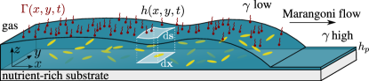
Figure 1: Sketch of a bacterial colony covered by an insoluble surfactant with concentration $\Gamma(x,y,t)$. The field $h(x,y,t)$ describes the height of liquid and biomass. The surfactant concentration on the colony is higher then on the surrounding substrate, resulting in gradients in the liquid-gas surface tension and outward-pointing Marangoni flows that promote the expansion of the colony.

A bacterial colony is a complex fluid, composed of water, bacteria, nutrients and molecules, which are secreted by the bacteria, e.g. extracellular polymeric substances and surfactants. In this work, we follow a simple two-field modelling strategy that allows for a selective study of the influence of wettability and Marangoni fluxes on the spreading dynamics. We treat the bacterial colony as a thin film of height $h(x,y,t)$ covered by insoluble surfactant molecules of concentration $\Gamma(x,y,t)$ [see Fig. 1]. To model the surfactant-driven spreading of the colony, we supplement the hydrodynamic description with bioactive growth processes for the film height $h$ and the surfactant concentration $\Gamma$. This approach is valid in the limit of fast osmotic equilibration between the colony and the agar substrate.Trinschek et al. (2017) Similar models - which represent just one class in the very rich literature concerning the mathematical modelling of bacterial colonies (for reviews see for example Wang and Zhang, 2010; Klapper and Dockery, 2010; Horn and Lackner, 2014; Picioreanu and Van Loosdrecht, 2003) - are used to study the influence of wettability Trinschek et al. (2016, 2017), quorum sensing Ward and King (2012); Ward et al. (2001) and the surfactant-driven spreading of bacterial colonies.Angelini et al. (2009); Fauvart et al. (2012)
In the following, we first present the ’passive’ part of the hydrodynamic model for thin, surfactant-covered films before introducing the bioactive terms.

II.1 Passive part of the model

We consider a thin film of height $h(x,y,t)$ which is covered by an insoluble surfactant of (area-)density $\Gamma(x,y,t)$. The description of the passive part of the model is based on the free energy functional

$$F[h,\Gamma]=\int\left[f_{w}(h)+f_{s}\left(\Gamma\right)\zeta\right]\mathrm{d\mathbf{x}}$$ (1)

with

$$\zeta=\sqrt{1+|\nabla h|^{2}}\approx 1+\tfrac{1}{2}|\nabla h|^{2}\,.$$ (2)

$F[h,\Gamma]$ in (1) contains the wetting energy $f_{w}(h)$ and the local free energy of the surfactant-covered free surface $f_{s}(\Gamma)$. Here, $\mathrm{d\mathbf{s}}=\zeta\mathrm{d\mathbf{x}}$ is the surface element of the curved liquid surface and $\mathrm{d\mathbf{x}}$ is the surface element of the euclidean flat substrate plane as depicted in Fig. 1. A common choice for the wetting energy isPismen (2006)

$$f_{w}(h)=A\left(-\frac{1}{2h^{2}}+\frac{h_{a}^{3}}{5h^{5}}\right)\,,$$ (3)

which combines destabilizing long-range van-der-Waals and stabilizing short-range interactions. It describes a partially wetting fluid, i.e. a macroscopic drop sitting on a stable adsorption layer of thickness $h_{a}$.
Assuming relatively low densities of surfactant, the contribution of a non-interacting surfactant to the energy of the interface corresponds to an entropic term

$$f_{s}(\Gamma)=\gamma+\frac{kT}{a^{2}}\Gamma\left[\log(\Gamma)-1\right]$$ (4)

that results in the usual linear equation of state. Here, $\gamma$ denotes the surface tension, $kT$ the thermal energy and $a^{2}$ is the effective area of the surfactant molecules on the interface. In order to write evolution equations for the film height and the surfactant concentration in the formulation as a gradient dynamics Thiele et al. (2012, 2016), it is necessary to introduce the projection of the area density onto the flat surface of the substrate

$$\tilde{\Gamma}(x,y,t)=\zeta\Gamma(x,y,t)\,.$$ (5)

The free energy functional (1) can now be used to write evolution equations for $h(x,y,t)$ and $\tilde{\Gamma}(x,y,t)$

$$\partial_{t}h=\nabla\cdot\left[Q_{hh}\nabla\frac{\delta F}{\delta h}+Q_{h\Gamma}\nabla\frac{\delta F}{\delta\tilde{\Gamma}}\right]$$ (6)

$$\partial_{t}\tilde{\Gamma}=\nabla\cdot\left[Q_{\Gamma h}\nabla\frac{\delta F}{\delta h}+Q_{\Gamma\Gamma}\nabla\frac{\delta F}{\delta\tilde{\Gamma}}\right]$$ (7)

with the positive definite mobility matrix Thiele et al. (2012); Wilczek et al. (2015)

$$\mathbf{Q}=\begin{pmatrix}Q_{hh}&Q_{\Gamma h}\\ Q_{h\Gamma}&Q_{\Gamma\Gamma}\end{pmatrix}=\begin{pmatrix}\frac{h^{3}}{3\eta}&\frac{h^{2}\Gamma}{2\eta}\\ \frac{h^{2}\Gamma}{2\eta}&\frac{h\Gamma^{2}}{\eta}+D\Gamma\end{pmatrix}\,,$$ (8)

where $\eta$ denotes the viscosity of the fluid and $D$ is the diffusivity of surfactant molecules on the interface. Performing the variations of the free energy functional and considering the thin film limit $\zeta\approx 1$ gives

$$\tfrac{\delta F}{\delta h} =\partial_{h}f_{w}-\nabla\left[\omega\nabla h\right]$$ (9)

$$\tfrac{\delta F}{\delta\Gamma} =\partial_{\Gamma}f_{s}\,.$$ (10)

with $\omega=f_{s}-\Gamma\partial_{\Gamma}f_{s}=\gamma-\frac{kT}{a^{2}}\Gamma$. Using the common approximation that the change of the surface tension with surfactant concentration is small as compared to the reference surface tension $\gamma$ (i.e. $\nabla\left[\omega\nabla h\right]\approx\gamma\Delta h$ ), we obtain

$$\partial_{t}h=\nabla\cdot\left[Q_{hh}\nabla[\partial_{h}f_{w}-\gamma\Delta h]+Q_{h\Gamma}\nabla(\partial_{\Gamma}f_{s})\right]$$ (11)

$$\partial_{t}\Gamma\approx\partial_{t}\tilde{\Gamma}=\nabla\cdot\left[Q_{\Gamma h}\nabla[\partial_{h}f_{w}-\gamma\Delta h]+Q_{\Gamma\Gamma}\nabla(\partial_{\Gamma}f_{s})\right]\,.$$ (12)

The last term of (11) corresponds to the negative of the Marangoni flux $\vec{j}_{M}=-\frac{kT}{2\eta a^{2}}h^{2}\nabla\Gamma$ - a flux in the fluid which is driven by concentration gradients of the surfactant.

II.2 Model for surfactant-driven colony spreading

In order to describe the surfactant-driven spreading of bacterial colonies, the hydrodynamic model equations for passive fluids (11)-(12) are extended by biological growth and production processes. Over time, bacteria will multiply by cell division and possibly secrete osmolytes. This may result in an influx of water into the colony caused by the difference of the osmotic pressures in the film and the underlying moist substrate.Seminara et al. (2012) We assume that this influx is fast as compared to the growth processes, which allows us to write biomass production and osmotic influx as one effective growth term $G(h)$. To account for processes such as nutrient and oxygen depletion Zhang et al. (2014); Dietrich et al. (2013) which naturally limit the colony height, we introduce a critical film height $h^{\star}$, which corresponds to the maximal height that can be sustained. It can be related to a local equilibrium of vertical nutrient diffusion and consumption by bacteria.Zhang et al. (2014) We assume a simple logistic growth law

$$G(h) =gh\left(1-\frac{h}{h^{\star}}\right)f_{mod}(h)$$ (13)

which is modified locally for very small amounts of biomass by $f_{mod}(h)$ in order to prevent proliferation in the adsorption layer outside of the colony and accounts for the fact that at least one bacterium is needed to start biomass growth.
The second bioactive process that needs to be included in the model is the production of surfactants by the bacteria. Due to the small height of the colony as compared to its lateral extension, the surfactant quickly diffuses to the liquid-air interface. We thus assume the production rate of surfactant $P(h,\Gamma)$ to be proportional to the biofilm height, to decrease with increasing surfactant concentration and to cease when the local surfactant concentration reaches a limiting value $\Gamma_{\text{max}}$:

$$P(h,\Gamma)=p(\Gamma_{\text{max}}-\Gamma)\Theta(\Gamma_{\text{max}}-\Gamma)\cdot h\Theta(h-h_{u})\,.$$ (14)

The step-functions $\Theta$ are introduced to ensure that production only takes place inside the colony and not in the adsorption layer and that surfactant above the maximal concentration $\Gamma_{\mathrm{max}}$ is not degraded.
We include biomass growth (13) and surfactant production (14) as additional non-conserved terms into the evolution equations (11)-(12)

$$\partial_{t}h= \nabla\cdot\left[\tfrac{h^{3}}{3\eta}\nabla(\partial_{h}f_{w}-\gamma\Delta h)\right]+\tfrac{kT}{a^{2}}\nabla\cdot\left[\tfrac{h^{2}}{2\eta}\nabla\Gamma\right]+G(h)$$ (15)

$$\partial_{t}\Gamma= \nabla\cdot\left[\tfrac{h^{2}\Gamma}{3\eta}\nabla(\partial_{h}f_{w}-\gamma\Delta h)\right]+\tfrac{kT}{a^{2}}\nabla\cdot\left[\tfrac{h\Gamma}{\eta}\nabla\Gamma\right]$$

$$+\tfrac{kT}{a^{2}}D\Delta\Gamma+P(h,\Gamma)$$ (16)

where we have used (4) and (8).

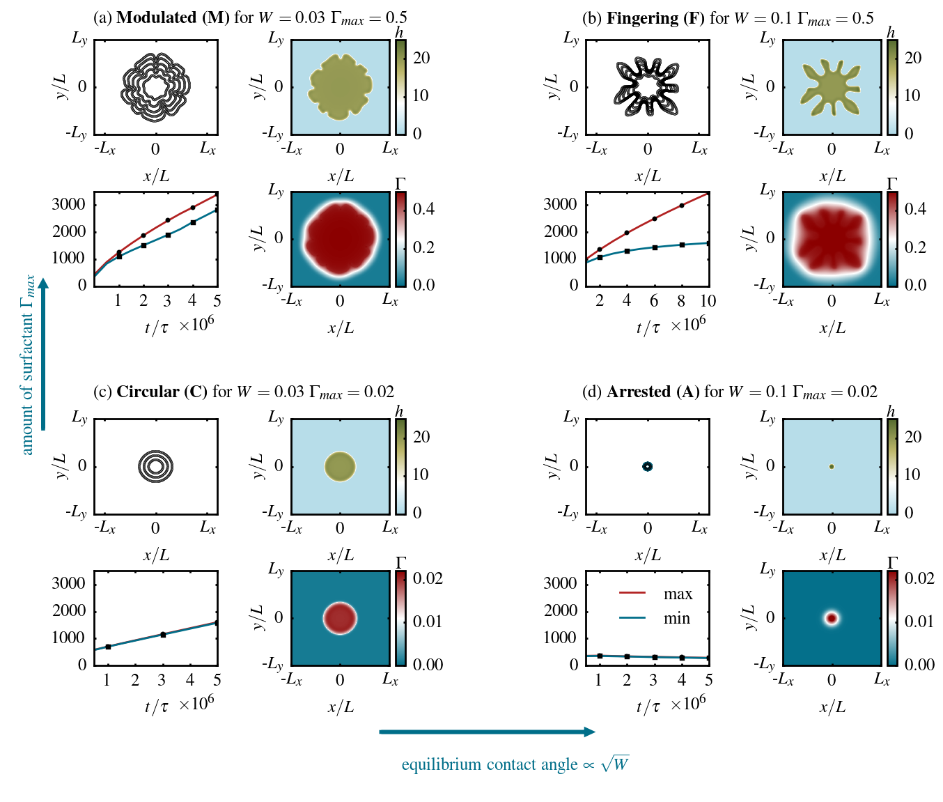
Figure 2: Panels (a) to (d) show the four different types of spreading that may occur depending on the wettability parameter $W$ and the maximal surfactant concentration $\Gamma_{\mathrm{max}}$. The resp. bottom left plots show the time dependence of the mean values of the maximal and minimal radii of the colony while the resp. top left plots show snapshots of the $h(x,y)=0.5h^{\star}$ contour line at the times indicated by filled symbols in the bottom left plots. The resp. top and bottom right plots show the film height and surfactant distribution, respectively, at the end of the simulation. Without surfactant, the shape of the bacterial colony is circular. At high wettability (c), the biofilm expands over the substrate with a stable circular front. Under conditions, which do not favour wetting (d), the spreading of the colony is arrested. If the colony produces a significant amount of surfactant $\Gamma_{\mathrm{max}}$, spreading is promoted by Marangoni fluxes and the circular front becomes unstable. For a high wettability (a), the front continuously advances but is modulated. For a higher value of $W$ (b), the colony forms pronounced fingers which expand over the substrate while the troughs stay arrested.

II.3 Non-dimensional form of the equations

To obtain a dimensionless form of the model (15)-(16) and thereby facilitate the analysis, we introduce the scaling

$$t=\tau\tilde{t}\qquad x=L\tilde{x}\qquad y=L\tilde{y}\qquad h=l\tilde{h}\qquad f_{w,s}=\kappa\tilde{f}_{w,s}$$ (17)

where a tilde indicates dimensionless quantities. Time, energy and vertical and horizontal length scales are

$$\tau=\tfrac{L^{2}\eta}{\kappa l}\qquad\kappa=\tfrac{kT}{a^{2}}\qquad l=h_{a}\qquad L=\sqrt{\tfrac{\gamma}{\kappa}}l\,,$$ (18)

respectively, and will be estimated quantitatively later in Sec. III.1. Inserting the scaling, into the evolution equation results in the dimensionless biomass growth rate $\tilde{g}=\tau g$, the dimensionless surfactant production rate $\tilde{p}=\tau pl$ and the wettability parameter

$$W=\frac{Aa^{2}}{h_{a}^{2}k_{B}T}\,,$$ (19)

which defines the relative strength of wetting as compared to the entropic influence of the surfactant. It is connected to the equilibrium contact angle $\theta_{e}$ of passive stationary droplets (without bio-active terms) by $\theta_{e}\propto\sqrt{W}$ so that larger values of $W$ result in a less wettable substrate and larger contact angles. If not stated otherwise, we fix the parameters to $\tilde{g}=10^{-5}$, $\tilde{p}=10^{-6}$, $h^{\star}=20.$ and $\tilde{D}=0.01$ throughout the analysis and study the effect of the wettability parameter $W$ and the maximal surfactant concentration $\Gamma_{\mathrm{max}}$ which captures e.g. the difference between a surfactant-producing bacterial strain and a mutant strain deficient in surfactant production.

III Results

In the next section, we present an analysis of the model which focuses on the influence of surfactants and wettability on the spreading dynamics and morphology. We start by performing time simulations of initially circular colonies at different parameter values $W$ and limiting surfactant concentrations $\Gamma_{\mathrm{max}}$ as illustrative examples and a graphic description of the effects. These can already be employed to gain a qualitative understanding of the spreading behaviour. In a next step, the spreading regimes are studied for planar fronts by parameter continuation techniques Doedel and Oldeman (2009). This results in a more technical description and facilitates, e.g., the analysis of the emerging front instability by a transversal linear stability analysis. The last part of this section contains an illustrative application of the model and exemplarily tests counter-gradients of surfactant as a strategy to arrest the expansion of bacterial colonies.

III.1 Influence of wettability and Marangoni fluxes on the morphology of fronts in radial geometry

In a first step, the front dynamics of model (15)-(16) is analysed by performing two-dimensional numerical time simulations of colony growth. These reveal the influence of wettability and the strength of the Marangoni fluxes on the morphology of the emerging bacterial colonies. We employ a finite element scheme provided by the modular toolbox DUNE-PDELABBastian et al. (2008a, b). The simulation domain $\Omega=[-L_{x},L_{x}]\times[-L_{y},L_{y}]$ with $L_{x}=L_{y}=5000$ is discretized on a regular mesh using $N_{x}\times N_{y}=512\times 512$ grid points and linear ansatz and test functions. The time-integration is performed using an implicit second order Runge-Kutta scheme with adaptive time step. On the boundaries, we apply no-flux conditions for film height and surfactant. The initial condition is given by a small nucleated bacterial colony with surfactant concentration $\Gamma_{\mathrm{max}}$ on the colony and $0.05\times\Gamma_{\mathrm{max}}$ on the surrounding substrate. The step functions in the surfactant production term (14) are approximated by $\Theta(x)\approx\frac{1}{2}[1+\tanh(100x)]$ .

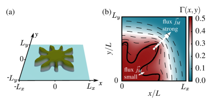
Figure 3: Details of the colony which spreads with pronounced fingers for $W=0.1$ and $\Gamma_{\mathrm{max}}=0.5$. (a) Height profile $h(x,y)$ at $t=10^{7}\tau$ reveals the rims which form at the edges of the fingers (cp. Fig. 2 (b)). (b) Surfactant concentration (colouring, dashed lines represent isolines) on a finger of the colony (solid black line). The gradient in surface tension and thus the Marangoni flux $\vec{j}_{M}$ is strong at the tips of the fingers, driving them further outwards. In the troughs, the surfactant concentration is at an overall high level so that the Marangoni flux is weak.

The time simulations of (15)-(16) reveal that - depending on the wettability and the strength of the Marangoni fluxes in the system - four qualitatively different types of spreading behaviour can occur. These are depicted in Fig. 2 (a) to (d) for four different choices of the parameters $W$ and $\Gamma_{\mathrm{max}}$. The respective top left plots show the contours of the colonies at equidistant times. The resp. bottom left plots in Fig. 2 give the time dependence of the mean values of the maximal and minimal radii of the colony to characterize its shape evolution. The resp. top and bottom right plots show the film height and surfactant distribution profiles at the end of the simulation.
We first discuss the spreading behaviour of the system for low surfactant densities (low $\Gamma_{\mathrm{max}}$). Consistent with the biofilm spreading model without surfactants in Trinschek et al., 2017, the system shows a non-equilibrium transition between continuously spreading and arrested colonies depending on the wettability parameter $W$. For small equilibrium contact angles and high wettability (low $W$, Fig. 2 (c)), the bacterial colony swells vertically and horizontally until the limiting film height $h^{\star}$ is reached. Subsequently, it spreads horizontally over the substrate with a constant speed and a circular (type C) colony shape. In contrast, at low wettability and thus high contact angle (high $W$, Fig. 2 (d)), the spreading of the bacterial colony is arrested (type A) and it evolves towards a steady profile of fixed extension and contact angle.
In both cases, the production of a significant amount of surfactant (high $\Gamma_{\mathrm{max}}$) improves the capability of the bacterial colony to expand outwards over the substrate. It results in a higher surfactant concentration $\Gamma(x,y)$ at the centre of the colony than on the surrounding substrate which induces an outwards flow due to the emerging surface tension gradient. For a continuously spreading colony, these Marangoni flows increase the spreading speed and also cause modulations (type M) of the circular colony shape to develop (low $W$, Fig. 2 (a)). However, eventually the growth of these undulations slows down and the tips and troughs of the front line translate with a similar velocity over the substrate. This can be clearly seen in the time evolution of the mean values of the maximal and minimal radii of the colony shape.
In the case of arrested spreading, the consequences of the surfactant production are even more drastic: In the first place it enables a horizontal expansion of the colony. Furthermore, it gives rise to the formation of pronounced fingers (high $W$, type F in Fig. 2 (b)). At large times, the finger tips spread outwards with a constant velocity whereas the troughs of the front line stay behind at a fixed position. A similar distinction of two types of front instabilities, for which the shape of the evolving front modulations becomes stationary (M) or corresponds to continuously growing fingers (F), has also been made for advancing coating films driven by gravity or shear stress.Eres et al. (2000) The mechanism behind the pronounced fingering mode found here becomes clear when studying the distribution of surfactant on the colony and the surrounding substrate in more detail. Fig. 3 (a) shows a height profile of a colony with pronounced fingers at $t=10^{7}\tau$. In agreement with the experimental observation Fauvart et al. (2012), we find a rim in the height profile at the edges of the colony that is particularly pronounced at the tips of the fingers. Due to the limiting film height $h^{\star}$, the centre of the colony is relatively flat. The surfactant concentration is shown in Fig. 3 (b) and allows one to understand the formation of the pronounced fingers. In the troughs close to the centre of the colony, the surfactant concentration is overall high and gradients in $\Gamma$ are small. This results in only small Marangoni fluxes which do not suffice to overcome the arrested spreading behaviour. In contrast, at the tips of the fingers, gradients in $\ Gamma$ and Marangoni fluxes are strong, driving the finger tips further outwards. If the diffusion of the surfactant is not too high, this gradient in $\Gamma$ is maintained, enabling the fingers to continuously spread over the substrate.
To see if our model predicts a reasonable spreading speed, we estimate the scales for time and length scales by comparing the numerically obtained extensions with experimental measurements and plug in numbers for the remaining constants in the model. The typical colony height of $15-25\,\mu$m as measured in Fauvart et al., 2012, sets the vertical length scale to $l=h_{a}\approx 1\,\mu$m. Together with the viscosity of $\eta\approx 0.1$ Pa s Fauvart et al. (2012) and surface tension of water $\gamma\approx 70$ mN/m, as well as a typical surfactant length scale $a\approx 3\,$nm, we find the lateral length scale $L\approx 10\mu$m and the time scale $\tau\approx 0.03$s. With the above scales, our numerically measured dimensionless expansion rate of roughly $5\times 10^{-4}$ in Fig. 2 (a) corresponds to a speed of about $10\mu$m/min, which compares well to the experimentally found value of $5-40\mu$m/min.Fauvart et al. (2012)
To obtain a more complete picture of the front instability, we also study the effect of the remaining parameters $\tilde{g}$, $\tilde{p}$, $h^{\star}$ and $\tilde{D}$ on the colony shape. We find that a small biomass growth rate $\tilde{g}$ as well as a small maximal biofilm thickness $h^{\star}$ promote the instability. Images from the direct time simulations can be found in appendix A1.

III.2 Profile and velocity of fronts in planar geometry

The time simulations of the two-dimensional system have identified the wettability parameter $W$ and the amount of surfactant $\Gamma_{\mathrm{max}}$ as two key parameters which influence the spreading of the bacterial colony. To understand the system in more detail, next we investigate planar fronts. In this geometry, it is possible to perform a more systematic analysis of the system using parameter continuation. This technique allows for a direct observation of the influence of $W$ and $\Gamma_{\mathrm{max}}$ on the front profile and velocity. To that end, the evolution equations (15)-(16) are transformed into the co-moving coordinate system with a constant velocity $v$

$$\partial_{t}h= \nabla\cdot\left[Q_{hh}\nabla[\partial_{h}f_{w}-\gamma\Delta h]+Q_{h\Gamma}\nabla(\partial_{\Gamma}f_{s})\right]$$

$$+G(h)+v\partial_{x}h$$ (20)

$$= \mathscr{F}_{1}(\nabla,v)[h,\Gamma]$$

$$\partial_{t}\Gamma= \nabla\cdot\left[Q_{\Gamma h}\nabla[\partial_{h}f_{w}-\gamma\Delta h]+Q_{\Gamma\Gamma}\nabla(\partial_{\Gamma}f_{s})\right]$$

$$+P(h,\Gamma)+v\partial_{x}\Gamma$$ (21)

$$= \mathscr{F}_{2}(\nabla,v)[h,\Gamma]\,,$$

where we introduced $\mathscr{F}_{1,2}(\nabla,v)$ as a short hand notation for the nonlinear operators defined by the right-hand sides of the evolution equations (20) and (21). In the co-moving frame, planar fronts $(h_{0}(x),\Gamma_{0}(x))$ which depend only on one spatial coordinate, $x$, and move with a stationary profile and velocity $v$ correspond to steady solutions

$$\partial_{t}h_{0}(x) =\mathscr{F}_{1}(\nabla,v)[h_{0}(x),\Gamma_{0}(x)]=0$$ (22)

$$\partial_{t}\Gamma_{0}(x) =\mathscr{F}_{2}(\nabla,v)[h_{0}(x),\Gamma_{0}(x)]=0\,,$$ (23)

and can thus be analysed by parameter continuation techniques Dijkstra et al. (2014); Kuznetsov (2013). To that end, we use the software package AUTO-07pDoedel and Oldeman (2009) which has previously been successfully employed for thin-film models, e.g. for dewetting simple and complex liquids Thiele et al. (2013), pattern formation in dip-coating Wilczek et al. (2016) or osmotically spreading biofilms.Trinschek et al. (2016, 2017) We impose that far away from the colony, the surfactant concentration is fixed to a small but finite value.

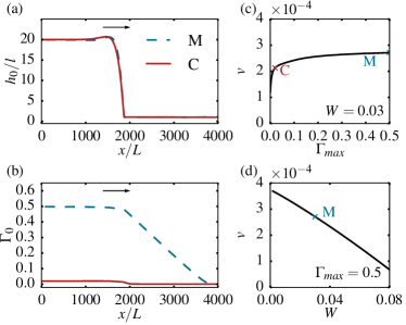
Figure 4: Shape and velocity of planar fronts. (a) and (b): Front profiles for parameter combinations corresponding to the circular (C) colony ($W=0.03$, $\Gamma_{\mathrm{max}}=0.02$) and the colony with the modulated (M) front shape ($W=0.03$, $\Gamma_{\mathrm{max}}=0.5$). The front velocity $v$ strongly depends on the maximal surfactant amount $\Gamma_{\mathrm{max}}$ (c) as well as the wettability parameter $W$ (d).

Fig. 4 (a) and (b) show the front profiles $(h_{0}(x),\Gamma_{0}(x))$ for the parameter combinations corresponding to modulated (M) and circular (C) spreading in the radial geometry (Fig 2). Behind the spreading front, $h$ and $\Gamma$ reach their saturation values $h^{\star}$ and $\Gamma_{\mathrm{max}}$, respectively. The height profile of the front shows a typical capillary rim. The surfactant diffuses in front of the moving colony, resulting in a linear decay. This is a typical profile, as discussed more generally in Williams and Jensen, 2001 for a moving source of surfactant.
The velocity of the front is strongly affected by the surfactant concentration $\Gamma_{\mathrm{max}}$ and the wettability parameter $W$ (see Figs. 4 (c) and (d)). For a bacterial colony with very small $\Gamma_{\mathrm{max}}$, e.g. a mutant strain deficient in surfactant production, the front velocity is roughly a factor of two smaller then in a colony with $\Gamma_{\mathrm{max}}=0.5$. This shows that the Marangoni effect gives a strong contribution to the outward flux that results in the colony expansion. In analogy to the transition from continuous to arrested spreading observed in biofilms without Marangoni flows Trinschek et al. (2017), the biofilm expansion slows down as the conditions do not favour wetting for large $W$.

In the time simulations for radial geometry discussed in section III.1, we found that the surfactant not only influences the spreading speed of the colonies, but also affects its morphology. We will focus on this aspect in the next section.

III.3 Transversal linear stability analysis of two-dimensional planar fronts

Now, we analyse the evolution of the morphology of planar fronts in a two-dimensional geometry. To that end, we perform a linear transversal stability analysis employing the ansatz

$$h(x,y,t) =h_{0}(x)+\epsilon h_{1}(x)\exp(ik_{y}y+\sigma t)$$ (24)

$$\Gamma(x,y,t) =\Gamma_{0}(x)+\epsilon\Gamma_{1}(x)\exp(ik_{y}y+\sigma t)$$ (25)

with $\epsilon\ll 1$. This corresponds to fronts consisting of a $y$-invariant base state given by the stationary fronts $(h_{0}(x),\Gamma_{0}(x))$ plus a small perturbation with $x$-dependence $(h_{1}(x),\Gamma_{1}(x))$ which is modulated in the $y$-direction with a wavenumber $k_{y}$ and grows or decays exponentially in time with the rate $\sigma$. Inserting this ansatz into the evolution equations (20)-(21) one obtains to $O(\epsilon)$ the linear eigenvalue problem

$$\sigma h_{1}(x) =\mathscr{F}_{1h}^{\prime}|_{h_{0}(x),\Gamma_{0}(x)}h_{1}(x)+\mathscr{F}_{1\Gamma}^{\prime}|_{h_{0}(x),\Gamma_{0}(x)}\Gamma_{1}(x)$$ (26)

$$\sigma\Gamma_{1}(x) =\mathscr{F}_{2h}^{\prime}|_{h_{0}(x),\Gamma_{0}(x)}h_{1}(x)+\mathscr{F}_{2\Gamma}^{\prime}|_{h_{0}(x),\Gamma_{0}(x)}\Gamma_{1}(x)\,,$$ (27)

for eigenvalues $\sigma$ and eigenfunctions $(h_{1}(x),\Gamma_{1}(x))$, where $\mathscr{F}^{\prime}_{i,h}$ and $\mathscr{F}^{\prime}_{i,\Gamma}$ are operators denoting the Fréchet-derivatives of the non-linear operator $\mathscr{F}_{i}$ with respect to $h$ and $\Gamma$, respectively. Statements about the linear stability of the front $(h_{0}(x),\Gamma_{0}(x))$ can now be made determining the largest eigenvalue $\sigma$ which tells if the perturbation grows (for $\sigma>0$) or decays (for $\sigma<0$) in time. The linear eigenvalue problem (26)-(27) is again solved using continuation techniques. The set of equations for the steady front profiles $h_{0}(x)$ and $\Gamma_{0}(x)$ employed in section III.2 is supplemented by a set of equations for the eigenfunctions that fulfill the same boundary conditions as the base state. This approach, in which transversal wave number and eigenvalue are treated as parameters in an pseudo-arclength continuation, is presented in tutorial form in Ref. Thiele, 2015.

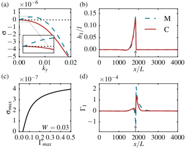
Figure 5: Linear transversal stability analysis for planar fronts in the co-moving frame for $W=0.03$. The dispersion relation shown in (a) monotonically decreases for $\Gamma_{\mathrm{max}}=0.02$ (red) but has a maximum $\sigma_{\mathrm{max}}>0$ for $\Gamma_{\mathrm{max}}=0.5$ (blue) indicating a front that is unstable with respect to transversal perturbations. (b) and (d) show the eigenfunctions for the fronts profiles in Fig. 4 corresponding to the transversal wave number $k_{y}$ with the largest eigenvalue. The grey arrow indicates the front position of the corresponding $h$ profiles. Following the maximum of the dispersion relation $\sigma_{\mathrm{max}}$ depending on $\Gamma_{\mathrm{max}}$ in (c) shows that for $W=0.03\textsection,$ the front profile is unstable for $\Gamma_{\mathrm{max}}>0.0268$.

We again investigate the front profiles for two parameter sets which correspond to the modulated (M) and circular (C) spreading in the radial geometry (Fig. 2). Recall that the respective base states $(h_{0}(x),\Gamma_{0}(x))$ are displayed in Fig. 4. In order to determine the transversal stability of these fronts, one needs to analyse the corresponding dispersion relations $\sigma(k_{y})$ which are shown in Fig. 5 (a). For the parameter set (C) with only a small concentration of surfactant $\Gamma_{\mathrm{max}}=0.02$, the dispersion relation decays monotonically (red solid line in Fig. 5 (a)). The largest eigenvalue is $\sigma_{\mathrm{max}}=0$ at $k_{y}=0$ and the front is thus transversally stable. The eigenfunction $(h_{1}(x),\Gamma_{1}(x))$ corresponding to the largest eigenvalue (red solid lines in Fig. 5 (b),(d)) is the neutrally stable (Goldstone) mode representing the translational symmetry of the equations. As expected, it is identical to the spatial derivative of the front profiles (data not shown).
For the other parameter set (M), which corresponds to the situation that a significant amount of surfactant $\Gamma_{\mathrm{max}}=0.5$ is present in the system, the largest eigenvalue is positive at finite wavenumber ($\sigma_{\mathrm{max}}=3.98\times 10^{-7}$ at $k_{y}=4.89\times 10^{-3}$) and the front is thus transversally unstable (blue dashed line in Fig. 5 (a)). These values roughly agree with linear results extracted from the fully nonlinear time simulation in a planar (data not shown). The eigenfunctions corresponding to the largest eigenvalue (blue dashed lines in 5 (b),(d)) are strongly localized in the front region (compare to Fig. 4). To find the surfactant concentration at which the transition from transversally stable to unstable fronts takes place, we follow the maximum of the dispersion relation $\sigma_{\mathrm{max}}$ while varying $\Gamma_{\mathrm{max}}$ (Fig. 5 (c)). At $W=0.03$, we find that $\sigma_{\mathrm{max}}$ is positive and the front profile thus transversally unstable for $\Gamma_{\mathrm{max}}>0.0268$.

III.4 Comparison to surfactant-driven spreading of ’passive’ thin films

The front profiles observed in our model show some of the main characteristics of the solutions observed for surfactant-driven spreading of passive thin liquid films as e.g. the capillary rim near the edge of the front and the linear decay of the surfactant concentration in front of the drop. In contrast to other modelling approaches Jensen and Naire (2006); Craster and Matar (2006); Warner et al. (2004), we incorporate a wetting energy corresponding to a partially wetting fluid, resulting in a stable adsorption layer of height $h_{a}$ independent of the surfactant concentration $\Gamma$. Therefore, we do not observe the typical fluid step or a thinned region in front of the advancing colony which is often described as the origin of the front instability observed for surfactant-driven spreading of ’passive’ drops on horizontal substrates.Matar and Craster (2009) Instead, our model for surfactant-driven colony spreading shows similarity to a surfactant covered drop sliding down an inclined substrate.Edmonstone et al. (2004, 2005); Goddard and Naire (2015) In this set-up, the spreading of the drop is - in addition to the Marangoni fluxes - driven by gravity which acts as a body force on the fluid. In our model, the driving is presented by the non-conserved biomass growth term. The fingering instability and the eigenfunctions of the unstable mode observed in our model strongly resemble the transversal perturbations found in a constant-flux configuration in Edmonstone et al., 2005 which are also located at the front edge rather than in the region ahead of it.

III.5 Phase-diagram for planar fronts

We complete our analysis of planar fronts by combining our results from the transversal linear stability analysis with time simulations. This allows us to determine a phase-diagram which distinguishes between different spreading modes depending on the wettability parameter $W$ and the surfactant concentration $\Gamma_{\mathrm{max}}$. The time simulations are performed on a domain $\Omega=[-L_{x},L_{x}]\times[-L_{y},L_{y}]$ with $L_{x}=1500$ and $L_{y}=3000$ discretized on an equidistant $N_{x}\times N_{y}=256\times 512$ mesh with the same integration method and boundary conditions as applied in section III.1. The initial condition consists of a noisy planar front given by the corresponding stationary front profile $(h_{0}(x),\Gamma_{0}(x))$ for each parameter set. The simulation time is $T_{\mathrm{end}}/\tau=10^{7}$. For initially planar fronts, we find three different spreading regimes as shown in Fig. 6: Arrested planar fronts, which do not advance (grey dots), moving planar fronts (red triangles) and moving modulated fronts (blue squares) for which the transversal perturbations $\Delta h$ grow in time (and thus $\frac{\Delta h(t=T_{\mathrm{end}})}{\Delta h(t=0)}>1$). We find the same tendencies as observed in the circular geometry in section III.1. At low surfactant concentration, the front spreads without a transversal instability for a small contact angle (low $W$) but is arrested for high $W$. An increased surfactant concentration leads to a modulated front. We compare this findings with the predictions from the transversal linear stability analysis. We identify the region in which the ansatz (24)-(25) of moving fronts is valid (stationary $h$ and $\Gamma$ in the co-moving frame) is valid. In the grey region to the right of the dashed line in Fig. 6, this condition breaks down and we do not expect a stationary moving front. This is in accordance with the occurrence of the arrested mode in the time simulations. Note that in this situation, the produced surfactant still spreads outwards and the arrested growth mode does therefore not correspond to a stationary front with $v=0$ for both fields $h$ and $\Gamma$. The transversal linear stability makes a prediction about the strength of the transversal instability via the largest eigenvalue $\sigma_{\mathrm{max}}$. To the left of the dotted line in Fig. 6, the eigenvalue is larger than $\sigma_{\mathrm{max}}=10^{-8}$ and the modulation of the front should be observable within our simulation time $T_{end}/\tau=5\cdot 10^{6}..10^{7}$. This is in good agreement with the time simulations.

Interestingly, the fingering mode (F) does not occur for time simulations initiated with planar fronts that are only slightly perturbed. In general, the transversal instability appears to be much weaker then observed in the radial geometry. This can be attributed to a dilution effect of the surfactant: In the radial geometry, the produced surfactant is diluted more strongly when it spreads outwards from the colony and the surfactant profile decays faster with the distance to the front. This results in stronger gradients in surfactant concentration which drive the transversal instability. To test if the fingering mode only exists for circular colonies, we perform the time simulations with an initial condition consisting of a planar front with a finite-size perturbation in the form of a small finger. We find that at large surfactant concentrations, the arrested spreading mode can be overcome (grey dots with white circle in Fig. 6): the initial finger continuously grows while the rest of the front stays behind similar to the radial geometry. In conclusion, the instability and especially the fingering mode are generically occurring in the planar and the radial geometry, however, the onset and strength critically depend on colony shape.

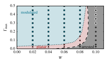
Figure 6: Phase-diagram for the spreading of two-dimensional planar fronts. To the left (right) of the dashed line, the fronts of the height profile $h$ are moving (not moving). The linear stability analysis predicts modulated moving fronts to the left of the dotted line (the largest eigenvalue $\sigma_{\mathrm{max}}$ is $>10^{-8}$). In numerical time simulations initiated with a noisy planar front, three types of spreading occur: transversally stable planar fronts (red triangles), modulated fronts (blue squares) and arrested fronts which can not expand over the substrate (grey dots). The grey dots with white circles mark parameter sets for which a finite perturbation in the initial condition leads to spreading of a pronounced finger.

III.6 Preventing the growth of bacterial colonies by a counter-gradient of surfactant

After analysing the model mathematically in sections III.2 to III.5, we illustrate the consequences of the spreading mechanism at an example. One strategy that has been suggested to arrest the expansion of a bacterial colony are counter-gradients of surfactants. Indeed, experimentsFauvart et al. (2012); Caiazza et al. (2005) show that spreading of a P. aeruginosa colony can be inhibited if exogenously added bio-surfactant is present on the agar substrate in a circular pattern around the colony with a concentration comparable to the in vivo one. To test this strategy in our model, we perform a time simulation with $W=0.1$ and $\Gamma_{\mathrm{max}}=0.5$ starting from an initial condition given by a surfactant-laden colony at the centre of the simulation domain and additional surfactant to the left of the colony. The time simulation (see Fig. 7) shows that the growth of the colony towards the left hand side slows down as soon as the colony ’senses’ the additional surfactant and eventually its growth is arrested. At the other side, the colony performs the expected finger-like growth. This effect can also be expected to occur when two surfactant-producing colonies approach each other, as observed experimentallyTremblay et al. (2007).

IV Conclusion and Outlook

We have developed and studied a simple model for surfactant-driven biofilm spreading which demonstrates that wettability and Marangoni fluxes have a strong effect on the expansion behaviour and morphology of bacterial colonies. The model we have presented is based on a hydrodynamic approach including wetting forces supplemented by bioactive terms and thus allows us to study the interplay between biological growth processes and passive surface forces. We find four different types of spreading, ranging from arrested spreading over circular spreading and undulated spreading fronts to the formation of pronounced fingers. The obtained results show that the production of bio-surfactants can enable a bacterial colony to spread over the substrate under conditions, which are otherwise unfavourable to a horizontal expansion; This is because the resulting Marangoni fluxes can significantly contribute to the spreading velocity. Our results are in qualitative agreement with the experimental findings Fauvart et al. (2012); Caiazza et al. (2005); Tremblay et al. (2007) which show that surfactant-producing Pseusomona aeruginosa colonies spread outwards and form pronounced fingers whereas a wild type deficient in surfactant production can not expand and is arrested in a small circular shape. This corresponds to the transition from the fingering mode to the arrested spreading mode that our model predicts.

Note that, here, capillarity and wettability on the one hand and the gradients in surface tension on the other hand have been treated separately in order to discuss their respective effects. In an experiment with bacterial colonies on agar plates, the wettability also depends on the concentration of surfactants because they alter the surface tension and thus the Hamaker constant (entering the parameter $W$)Thiele et al. (2018). Therefore, the difference between a bacterial strain deficient in surfactant production and a surfactant producing strain implies that the latter has a lower parameter $W$ and a higher surfactant concentration $\Gamma_{\mathrm{max}}$ (see discussion in Trinschek et al., 2017).
In this work, we have followed a simple two-field approach, treating the bacterial colony as a complex fluid covered by surfactants. To capture situations, in which variations of the colony composition are not negligible, e.g. because of similar time scales for biomass growth and osmotic processes, the model can be extended to a three-field model. There, the water concentration enters as a separate field as described in Trinschek et al., 2017. In addition, the extension of the model to soluble surfactants with a bulk concentration is straight forward, following the model for passive fluids presented in Thiele et al., 2016. Our modelling approach neglects complex features, such as vertical gradients or cell differentiation. Experiments Fauvart et al. (2012) in which the rhamnolipid production in Pseudomona aeruginosa colonies is highlighted by autofluorescence indicate that there are only small spatio-temporal variations in surfactant production throughout the colony but in general, cell differentiation is an important phenomenon in bacterial colonies and biofilmsVlamakis et al. (2008). In future extensions of the model, one may also incorporate the quorum sensing role of the bio-surfactants which allows for a basic form of communication between individual cells. However, as our model focuses on the physical effects of bio-surfactants, it is well suited to show that these suffice to induce the striking fingering colony shapes which are observed experimentally.

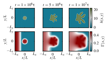
Figure 7: Inhibition of bacterial expansion by a counter-gradient of surfactant. Initially, surfactant is deposited on the left border of the computational domain, while a small drop of a bacterial colony is initiated in the centre. The counter-gradient of external surfactant inhibits fingering towards the left border. Parameters are $W=0.1$ and $\Gamma_{\mathrm{max}}=0.5$.

Conflict of interest

There are no conflicts to declare.

V Appendix

For completeness, we briefly investigate the influence of the remaining dimensionless parameters and test the robustness of the observed phenomena by performing additional numerical time simulations. A simulation with the parameters $W=0.05$, $\Gamma_{\mathrm{max}}=0.5$, $\tilde{g}=10^{-5}$, $\tilde{p}=10^{-6}$, $h^{\star}=20.$ and $\tilde{D}=0.01$ is used as a reference and each parameter is varied individually. Fig. 8 shows time simulations which are initiated with a quarter of a small bacterial colony with surfactant concentration $\Gamma_{\mathrm{max}}$ on a domain $\Omega=[0,5000]\times[0,5000]$ discretized on an equidistant mesh of $N_{x}\times N_{y}=256\times 256$ grid points. A larger biomass production rate $\tilde{g}$ reduces the formation of fingers as the hydrodynamic time-scale which is relevant for the Marangoni fluxes that drive the instability is no longer fast enough (see Fig.8 (a)). An increase of the limiting height $h^{\star}$ also results in a weakening of the instability (see Fig.8 (b)). A change of the surfactant diffusion $\tilde{D}$ or the production rate $\tilde{p}$ does not change the morphology of the colonies drastically (see Fig.8 (b) and (c), respectively).

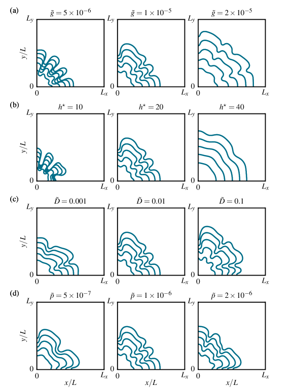
Figure 8: Parameter study to test the influence of the remaining parameters $\tilde{g}$, $h^{\star}$, $\tilde{D}$ and $\tilde{p}$ on the colony shape. The contour line $h(x,y)=0.5h^{\star}$ is shown at equidistant times with $\Delta t=10^{6}$. In each run, one parameter is varied as compared to a reference parameter set (middle column) with $W=0.05$, $\Gamma_{\mathrm{max}}=0.5$, $\tilde{g}=10^{-5}$, $\tilde{p}=10^{-6}$, $h^{\star}=20.$ and $\tilde{D}=0.01$.

References

- Donlan (2002) R. M. Donlan, Emerg. Infect. Dis. 8, 881 (2002).
- Stoodley et al. (2002) P. Stoodley, K. Sauer, D. G. Davies, and J. W. Costerton, Annu. Rev. Microbiol. 56, 187 (2002).
- Yang et al. (2017) A. Yang, W. S. Tang, T. Si, and J. X. Tang, Biophys. J. 112, 1462 (2017).
- Seminara et al. (2012) A. Seminara, T. Angelini, J. Wilking, H. Vlamakis, S. Ebrahim, R. Kolter, D. Weitz, and M. Brenner, Proc. Natl. Acad. Sci. U. S. A. 109, 1116 (2012).
- Trinschek et al. (2016) S. Trinschek, K. John, and U. Thiele, AIMS Materials Science 3, 1138 (2016).
- Dilanji et al. (2014) G. E. Dilanji, M. Teplitski, and S. J. Hagen, Proc. R. Soc. B 281, 1784 (2014).
- Yan et al. (2017) J. Yan, C. D. Nadell, H. A. Stone, N. S. Wingreen, and B. L. Bassler, Nature Comm. 8, 327 (2017).
- Ron and Rosenberg (2001) E. Z. Ron and E. Rosenberg, Environ. Microbiol. 3, 229 (2001).
- Raaijmakers et al. (2010) J. M. Raaijmakers, I. De Bruijn, O. Nybroe, and M. Ongena, FEMS Microbiol. Rev. 34, 1037 (2010).
- Ke et al. (2015) W.-J. Ke, Y.-H. Hsueh, Y.-C. Cheng, C.-C. Wu, and S.-T. Liu, Front Microbiol 6, 1017 (2015).
- Leclère et al. (2006) V. Leclère, R. Marti, M. Béchet, P. Fickers, and P. Jacques, Arch. Microbiol. 186, 475 (2006).
- Fauvart et al. (2012) M. Fauvart, P. Phillips, D. Bachaspatimayum, N. Verstraeten, J. Fransaer, J. Michiels, and J. Vermant, Soft Matter 8, 70 (2012).
- De Dier et al. (2015) R. De Dier, M. Fauvart, J. Michiels, and J. Vermant, “The role of biosurfactants in bacterial systems,” in The Physical Basis of Bacterial Quorum Communication, edited by S. Hagen (Springer, 2015) Chap. The Role of Biosurfactants in Bacterial Systems, pp. 189–204.
- Caiazza et al. (2005) N. C. Caiazza, R. M. Shanks, and G. O’toole, J. Bacteriol. 187, 7351 (2005).
- Daniels et al. (2006) R. Daniels, S. Reynaert, H. Hoekstra, C. Verreth, J. Janssens, K. Braeken, M. Fauvart, S. Beullens, C. Heusdens, I. Lambrichts, et al., Proc. Natl. Acad. Sci. USA 103, 14965 (2006).
- Be’er et al. (2009) A. Be’er, R. S. Smith, H. Zhang, E.-L. Florin, S. M. Payne, and H. L. Swinney, J. Bacteriol. 191, 5758 (2009).
- Kinsinger et al. (2003) R. F. Kinsinger, M. C. Shirk, and R. Fall, J. Bacteriol. 185, 5627 (2003).
- Angelini et al. (2009) T. Angelini, M. Roper, R. Kolter, D. A. Weitz, and M. P. Brenner, Proc. Natl. Acad. Sci. USA 106, 18109 (2009).
- Tremblay et al. (2007) J. Tremblay, A.-P. Richardson, F. Lépine, and E. Déziel, Environ. Microbiol. 9, 2622 (2007).
- Matar and Craster (2009) O. K. Matar and R. V. Craster, Soft Matter 5, 3801 (2009).
- Marmur and Lelah (1981) A. Marmur and M. D. Lelah, Chem. Eng. Commun. 13, 133 (1981).
- Troian et al. (1989) S. M. Troian, X. L. Wu, and S. A. Safran, Phys. Rev. Lett. 62, 1496 (1989).
- He and Ketterson (1995) S. He and J. Ketterson, Phys. Fluids 7, 2640 (1995).
- Cachile et al. (1999) M. Cachile, A. Cazabat, S. Bardon, M. Valignat, and F. Vandenbrouck, Colloids Surf., A 159, 47 (1999).
- Afsar-Siddiqui et al. (2003) A. B. Afsar-Siddiqui, P. F. Luckham, and O. K. Matar, Langmuir 19, 696 (2003).
- Afsar-Siddiqui et al. (2004) A. Afsar-Siddiqui, P. Luckham, and O. Matar, Langmuir 20, 7575 (2004).
- Troian et al. (1990) S. Troian, E. Herbolzheimer, and S. Safran, Phys. Rev. Lett. 65, 333 (1990).
- Matar and Troian (1999) O. K. Matar and S. M. Troian, Phys. Fluids 11, 3232 (1999).
- Warner et al. (2004) M. Warner, R. Craster, and O. Matar, Phys. Fluids 16, 2933 (2004).
- Craster and Matar (2006) R. Craster and O. Matar, Phys. Fluids 18, 032103 (2006).
- Marrocco et al. (2010) A. Marrocco, H. Henry, I. Holland, M. Plapp, S. Séror, and B. Perthame, Math Model Nat Phenom 5, 148 (2010).
- Thiele et al. (2012) U. Thiele, A. J. Archer, and M. Plapp, Phys. Fluids 24, 102107 (2012), note that a term was missed in the variation of and a correction is contained in the appendix of thap2016prf.
- Trinschek et al. (2017) S. Trinschek, K. John, S. Lecuyer, and U. Thiele, Phys. Rev. Lett. 119, 078003 (2017).
- Wang and Zhang (2010) Q. Wang and T. Zhang, Solid State Comm. 150, 1009 (2010).
- Klapper and Dockery (2010) I. Klapper and J. Dockery, SIAM Rev. 52, 221 (2010).
- Horn and Lackner (2014) H. Horn and S. Lackner, in Productive Biofilms, Advances in Biochemical Engineering/Biotechnology, Vol. 146, edited by K. Muffler and R. Ulber (Springer International Publishing, 2014) pp. 53–76.
- Picioreanu and Van Loosdrecht (2003) C. Picioreanu and M. Van Loosdrecht, “Biofilms in medicine, industry and environmental biotechnology - characteritics, analysis and control,” (IWA Publishing, 2003) Chap. Use of mathematical modelling to study biofilm development and morphology, pp. 413–438.
- Ward and King (2012) J. Ward and J. King, J. Eng. Math. 73, 71 (2012).
- Ward et al. (2001) J. Ward, J. King, A. Koerber, P. Williams, J. Croft, and R. Sockett, IMA J. Math. Appl. Med. Biol. 18, 263 (2001).
- Pismen (2006) L. M. Pismen, Patterns and interfaces in dissipative dynamics (Springer Science & Business Media, 2006).
- Thiele et al. (2016) U. Thiele, A. Archer, and L. Pismen, Phys. Rev. Fluids 1, 083903 (2016).
- Wilczek et al. (2015) M. Wilczek, W. B. H. Tewes, S. V. Gurevich, M. H. Köpf, L. Chi, and U. Thiele, Math. Model. Nat. Phenom. 10, 44 (2015).
- Zhang et al. (2014) W. Zhang, A. Seminara, M. Suaris, M. P. Brenner, D. A. Weitz, and T. E. Angelini, New J. Phys. 16, 015028 (2014).
- Dietrich et al. (2013) L. Dietrich, C. Okegbe, A. Price-Whelan, H. Sakhtah, R. Hunter, and D. Newman, J. Bacteriol. 195, 1371 (2013).
- Doedel and Oldeman (2009) E. J. Doedel and B. E. Oldeman, AUTO07p: Continuation and Bifurcation Software for Ordinary Differential Equations, Concordia University, Montreal (2009).
- Bastian et al. (2008a) P. Bastian, M. Blatt, A. Dedner, C. Engwer, R. Klöfkorn, R. Kornhuber, M. Ohlberger, and O. Sander, Computing 82, 103 (2008a).
- Bastian et al. (2008b) P. Bastian, M. Blatt, A. Dedner, C. Engwer, R. Klöfkorn, R. Kornhuber, M. Ohlberger, and O. Sander, Computing 82, 121 (2008b).
- Eres et al. (2000) M. H. Eres, L. W. Schwartz, and R. V. Roy, Phys. Fluids 12, 1278 (2000).
- Dijkstra et al. (2014) H. A. Dijkstra, F. W. Wubs, A. K. Cliffe, E. Doedel, I. F. Dragomirescu, B. Eckhardt, A. Y. Gelfgat, A. Hazel, V. Lucarini, A. G. Salinger, E. T. Phipps, J. Sanchez-Umbria, H. Schuttelaars, L. S. Tuckerman, and U. Thiele, Commun. Comput. Phys. 15, 1 (2014).
- Kuznetsov (2013) Y. A. Kuznetsov, Elements of applied bifurcation theory, Vol. 112 (Springer Science & Business Media, 2013).
- Thiele et al. (2013) U. Thiele, D. V. Todorova, and H. Lopez, Phys. Rev. Lett. 111, 117801 (2013).
- Wilczek et al. (2016) M. Wilczek, J. Zhu, L. Chi, U. Thiele, and S. V. Gurevich, J. Phys.: Condens. Matter 29, 014002 (2016).
- Williams and Jensen (2001) H. Williams and O. Jensen, IMA J. Appl. Math. 66, 55 (2001).
- Thiele (2015) U. Thiele, in Münsteranian Torturials on Nonlinear Science: Continuation, edited by U. Thiele, O. Kamps, and S. V. Gurevich (CeNoS, Münster, 2015) 1st ed.
- Jensen and Naire (2006) O. Jensen and S. Naire, J. Fluid Mech. 554, 5 (2006).
- Edmonstone et al. (2004) B. Edmonstone, O. Matar, and R. Craster, J Eng Math 50, 141 (2004).
- Edmonstone et al. (2005) B. Edmonstone, O. Matar, and R. Craster, Physica D: Nonlinear Phenomena 209, 62 (2005).
- Goddard and Naire (2015) J. Goddard and S. Naire, J. Fluid Mech. 772, 535 (2015).
- Thiele et al. (2018) U. Thiele, J. H. Snoeijer, S. Trinschek, and K. John, arXiv preprint arXiv:1802.04042 (2018).
- Vlamakis et al. (2008) H. Vlamakis, C. Aguilar, R. Losick, and R. Kolter, Genes & development 22, 945 (2008).