Composable Planning with Attributes

Abstract

The tasks that an agent will need to solve often are not known during training. However, if the agent knows which properties of the environment are important then, after learning how its actions affect those properties, it may be able to use this knowledge to solve complex tasks without training specifically for them. Towards this end, we consider a setup in which an environment is augmented with a set of user defined attributes that parameterize the features of interest. We propose a method that learns a policy for transitioning between “nearby” sets of attributes, and maintains a graph of possible transitions. Given a task at test time that can be expressed in terms of a target set of attributes, and a current state, our model infers the attributes of the current state and searches over paths through attribute space to get a high level plan, and then uses its low level policy to execute the plan. We show in 3D block stacking, grid-world games, and StarCraft that our model is able to generalize to longer, more complex tasks at test time by composing simpler learned policies.

SE[DOWHILE]DoDoWhiledo[1]while #1

1 Introduction

Researchers have demonstrated impressive successes in building agents that can achieve excellent performance in difficult tasks, e.g. (mnih2015; Silver2016). However, these successes have mostly been confined to situations where it is possible to train a large number of times on a single known task. On the other hand, in some situations, the tasks of interest are not known at training time or the space of tasks is so large that an agent will not realistically be able to train many times on any single task in the space.

We might hope that the tasks of interest are compositional: for example, cracking an egg is the same whether one is making pancakes or an omelette. If the space of tasks we want an agent to be able to solve has compositional structure, then a state abstraction that exposes this structure could be used both to specify instructions to the agent, and to plan through sub-tasks that allow the agent to complete its instructions.

In this work we show how to train agents that can solve complex tasks by planning over a sequence of previously experienced simpler ones. The training protocol relies on a state abstraction that is manually specified, consisting of a set of binary attributes designed to capture properties of the environment we consider important. These attributes, learned at train time from a set of (state, attribute) pairs, provide a natural way to specify tasks, and a natural state abstraction for planning. Once the agent learns how its actions affect the environment in terms of the attribute representation, novel tasks can be solved compositionally by executing a plan consisting of a sequence of transitions between abstract states defined by those attributes. Thus, as in (Dayan_FN; Dietterich_MAXQ; VezhnevetsOSHJS17), temporal abstractions are explicitly linked with state abstractions.

Our approach is thus a form of model-based planning, where the agent first learns a model of its environment (the mapping from states to attributes, and the attribute transition graph), and then later uses that model for planning. In particular, it is not a reinforcement learning approach, as there is no supervision or reward given for completing the tasks of interest. Indeed, outside of the (state, attribute) pairs, the agent receives no other reward or supervision. In the experiments below, we will show empirically that this kind of approach can be useful on problems that can be challenging for standard reinforcement learning.

We evaluate compositional planning in several environments. We first consider 3D block stacking, and show that we can compose single-action tasks seen during training to perform multi-step tasks. Second, we plan over multi-step policies in 2-D grid world tasks. Finally, we see how our approach scales to a unit-building task in StarCraft.

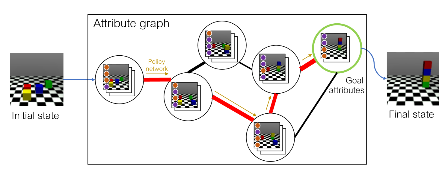
Figure 1: Solving complex tasks by planning in attribute space. Each state is mapped to a set of binary attributes (orange/purple dots) which is learned from a set of labeled (state, attribute) pairs provided as input. One attribute might mean, for example, “there is a blue block left of the red block”. The planning algorithm uses a graph over these sets of attributes with edge weights corresponding to the probability that a parametric policy network is able to transition from one attribute set to another. The graph and policy are learned during training via exploration of the environment. Given a goal attribute set (green), we use the graph to find the shortest path (red) to it in attribute space. The policy network then executes the actions at each stage (gold arrows).

2 The Attribute Planner Model

We consider an agent in a Markov environment, i.e. at each time the agent observes the state $s$ and takes action $a$, which uniquely determines the probability $P(s,a,s^{\prime})$ of transitioning from $s$ to $s^{\prime}$. We augment the environment with a map $f:S\to\{\rho\}$ from states to a set of user-defined attributes $\rho$. We assume that either $f$ is provided or a small set of hand-labeled $(s,\rho)$ pairs are provided in order to learning a mapping $\hat{f}$. Hence, the attributes are human defined and constitute a form of supervision. Here we consider attributes that are sets of binary vectors. These user-specified attributes parameterize the set of goals that can be specified at test time.

The agent’s objective at test time is, given a set of goal attributes $\rho_{g}$, to take a sequence of actions in the environment that end with the agent in a state that maps to $\rho_{g}$. During training, the agent constructs a model with three parts:

1. a neural-net based attribute detector $\hat{f}$, which maps states $s$ to a set of attributes $\rho$, i.e. $\rho=\hat{f}(s)$.

2. a neural net-based policy $\pi(s,\rho_{g})$ which takes a pair of inputs: the current state $s$ and attributes of an (intermediate) goal state $\rho_{g}$, and outputs a distribution over actions.

3. a transition table $c_{\pi}(\rho_{i},\rho_{j})$ that records the empirical probability that $\pi(s_{\rho_{i}},\rho_{j})$ can succeed at transiting successfully from $\rho_{i}$ to $\rho_{j}$ in a small number of steps.

The transition table $c_{\pi}$ can be interpreted as a graph where the edge weights are probabilities. This high-level attribute graph is then searched at test time to find a path to the goal with maximum probability of success, with the policy network performing the low-level actions to transition between adjacent attribute sets.

2.1 Training the Attribute Planner

The first step in training the Attribute Planner is to fit the neural network detector $\hat{f}$ that maps states $s$ to attributes $\rho$, using the labeled states provided. If a hardcoded function $f$ is provided, then this step can be elided.

In the second step, the agent explores its environment using an exploratory policy. Every time an attribute transition $(\rho_{i},\rho_{j})$ is observed, it is recorded in an intermediate transition table $c_{\pi_{e}}$. This table will be used in later steps to keep track of which transitions are possible.

The most naive exploratory policy takes random actions, but the agent can explore more efficiently if it performs count-based exploration in attribute space. We use a neural network exploration policy that we train via reinforcement learning with a count-based reward proportional to $c_{\pi_{e}}(\rho_{i},\rho_{j})^{-0.5}$ upon every attribute transition $(\rho_{i},\rho_{j})$, where $c_{\pi_{e}}(\rho_{i},\rho_{j})$ is the visit count of this transition during exploration. This bonus is similar to, for example, Model-based Interval Estimation with Exploration Bonuses (strehl2008analysis), but with no empirical reward from the environment. The precise choice of exploration bonus is discussed in Appendix LABEL:app:exploration.

Now that we have a graph of possible transitions, we next train the low-level goal-conditional policy $\pi$ and the main transition table $c_{\pi}$. From state $s$ with attributes $\rho$, the model picks an attribute set $\rho_{g}$ randomly from the neighbors of $\rho$ in $c_{\pi_{e}}$ weighted by their visit count in the Explore phase and sets that as the goal for $\pi$. Once the goal is achieved or a timeout is reached, the policy is updated and the main transition table $c_{\pi}$ is updated to reflect the success or failure. $\pi$ is updated via reinforcement learning, with a reward $r$ of $1$ if $\rho_{g}$ was reached and $0$ otherwise. See Algorithm 1 for pseudocode of AP training.

In the case of block stacking (Sec. LABEL:sec:stacking), the attribute transitions consist of a single step, so we treat $\pi$ as an “inverse model” in the style of (poking; AndrychowiczWRS17), and rather than using reinforcement learning, we can train $\pi$ in a supervised fashion by taking random actions and training $\pi$ to predict the action taken given the initial state and final attributes.

Algorithm 1 Attribute Planner Training

Input:Labeled pairs $\{(s_{i},\rho_{i})\}$, exploratory policy $\pi_{e}$, $N_{1}$, $N_{2}$, $t_{max}$. // Step 1: Train attribute detectorFit $\hat{f}$on $\{(s_{i},\rho_{i})\}$with supervised learning. // Step 2: Explore$t=1\ ...\ N_{1}$Act according to $\pi_{e}(s_{t-1})$. Compute attributes $\rho_{t}\leftarrow\hat{f}(s_{t})$$\rho_{t}\neq\rho_{t-1}$Record the transition: $c_{\pi_{e}}(\rho_{t-1},\rho_{t})\mathrel{{+}{=}}1$Optional: Update $\pi_{e}$with count-based reward. // Step 3: Train policy $\pi$ and $c_{\pi}$$t_{last}\leftarrow 0,\rho_{s}\leftarrow\emptyset,\rho_{e}\leftarrow\textrm{RandNeighbor}(c_{\pi_{e}},\rho_{s})$$t=1\ ...\ N_{2}$Compute attributes $\rho_{t}\leftarrow\hat{f}(s_{t})$$t=1$or $\rho_{t}\neq\rho_{s}$or $t-t_{last}\geq t_{max}$$r\leftarrow 1$if $\rho_{t}=\rho_{e}$, otherwise $0$. UpdatePolicy($\pi,r$) Record attempt: $A_{\pi}(\rho_{t-1},\rho_{t})\ \mathrel{{+}{=}}1$Record success: $S_{\pi}(\rho_{t-1},\rho_{t})\mathrel{{+}{=}}r$$\rho_{s}\leftarrow\rho_{t},\rho_{e}\leftarrow\textrm{RandNeighbor}(c_{\pi_{e}},\rho_{s})$$t_{last}\leftarrow t$Take an action according to $\pi(s_{t-1},\rho_{e})$$(\rho_{i},\rho_{j})\in A_{\pi}$$c_{\pi}(\rho_{i},\rho_{j})\leftarrow S_{\pi}(\rho_{i},\rho_{j})/A_{\pi}(\rho_{i},\rho_{j})$.

2.2 Evaluating the model

Once the model has been built we can use it for planning. That is, given an input state $s$ and target set of attributes $\rho_{T}$, we find a path $[\rho_{0},\rho_{1},...,\rho_{m}]$ on the graph $G$ with $\rho_{0}=f(s)$ and $\rho_{m}=\rho_{T}$ minimizing

$$\sum_{i=0}^{m-1}-\log c_{\pi}(\rho_{i},\rho_{i+1})$$ (1)

which maximizes the probability of success of the path (assuming independence). The probability $c_{\pi}$ is computed in Algorithm 1 as the ratio of observed successes and attempts during training.

The optimal path can be found using Dijkstra’s algorithm with a distance metric of $-\log(c_{\pi}(\rho_{i},\rho_{i+1}))$. The policy is then used to move along the resulting path between attribute set, i.e. we take actions according to $a=\pi(s,\rho_{1})$, then once $f(s)=\rho_{1}$, we change to $a=\pi(s,\rho_{2})$ and so on. At each intermediate step, if the current attributes don’t match the attributes on the computed path, then a new path is computed using the current attributes as a starting point (or, equivalently, the whole path is recomputed at each step).

Algorithm 2 Attribute Planner Inference

Input:Low-level policy $\pi$, graph $c_{\pi}$, attribute detector $\hat{f}$, target attributes $\rho_{T}$.